


1 Introduction
Lock-exchange flow at high Reynolds number has been widely analysed since it is representative of several natural flows and also shows interesting features connected to the mathematical aspects of the model. Gravity currents (GCs) are driven by the gradient pressure due to the different density of the current and the ambient fluid, and propagate in horizontal or inclined channels with regular or irregular cross-section. In many cases the Boussinesq approximation is adopted, neglecting the density variation in the inertial term, but in several other cases the difference in density between the current and the ambient fluid is relevant and a more complete model is required. In this respect, the classical top-lid configuration has interested numerous researchers (Gröbelbauer, Fanneløp & Britter Reference Gröbelbauer, Fanneløp and Britter1993; Lowe, Rottman & Linden Reference Lowe, Rottman and Linden2005; Jacobson & Testik Reference Jacobson and Testik2013; Birman, Martin & Meiburg Reference Birman, Martin and Meiburg2005; Étienne, Hopfinger & Saramito Reference Étienne, Hopfinger and Saramito2005; Ungarish Reference Ungarish2007; Bonometti, Balachandar & Magnaudet Reference Bonometti, Balachandar and Magnaudet2008; Ungarish Reference Ungarish2011; Bonometti, Ungarish & Balachandar Reference Bonometti, Ungarish and Balachandar2011; Rotunno et al. Reference Rotunno, Klemp, Bryan and Muraki2011; Turnbull & McElwaine Reference Turnbull and McElwaine2008; Dai Reference Dai2014). Further model refinements included a density stratification in the ambient fluid (Longo et al. Reference Longo, Ungarish, Di Federico, Chiapponi and Addona2016) and particulate GCs advancing in a stratified ambient fluid (Zemach et al. Reference Zemach, Chiapponi, Petrolo, Ungarish, Longo and Di Federico2017). In passing, we notice that most of these experiments were conducted without a top lid, but the configuration was such that the effects of the interface between the ambient fluid and the atmosphere were negligible. Particle-laden flows occurring in submarine canyons, and dry snow avalanches diffused in mountain areas are two examples of relevant natural GCs where the Boussinesq approximation does not hold (Ancey et al. Reference Ancey, Cochard, Wiederseiner and Rentschler2006). A second aspect of interest in the study of GCs is the role of the ambient fluid. The depth of the ambient fluid can be large enough to have negligible effects on the current dynamics; in this case a one-layer model is sufficient. If the thickness is of the same order as the intruding current, a two-layer model is required. In addition, the ambient fluid can be confined at the top (GCs with a top lid) or not, with an interface at atmospheric pressure. The correct modelling of GCs (i) with a high Reynolds number, (ii) flowing in an ambient fluid of limited depth under the non-Boussinesq regime and (iii) without a top lid requires further efforts.
Ungarish (Reference Ungarish2017) has developed a formal steady-state solution of the mathematical problem for a GC advancing at high Reynolds number in a rectangular horizontal channel with the upper surface of the ambient fluid open to the atmosphere. The front condition adopted is an extension of the classical Benjamin solution (Benjamin Reference Benjamin1968), the flow is generally dissipative (as a consequence of the jumps and discontinuities) and the results collapse to the classical results widely experimentally verified for GCs with a top lid in the Boussinesq regime. Ungarish (Reference Ungarish2017) has clearly answered the question as to whether the constraint of a top lid limiting the ambient fluid is essential or not for the development of a mathematical solution following the same path of Benjamin’s solution, a model followed by numerous researchers: it is not essential, providing a reformulation of the problem. The model described in Ungarish (Reference Ungarish2017) has been validated by physical experiments and with numerical computational fluid dynamics models (Longo et al. Reference Longo, Ungarish, Di Federico, Chiapponi and Petrolo2018), confirming within the usual accuracy the theoretical predictions of front speed and amplitude and wavelength of the free-surface depression. Experiments in similar conditions have been carefully conducted and documented in Sciortino, Adduce & Lombardi (Reference Sciortino, Adduce and Lombardi2018), obtaining similar results.
A subsequent analysis by Ungarish (Reference Ungarish2019) has extended the theoretical model to a channel with a cross-section of generic shape. The extension is far from trivial, since while for a rectangular channel a two-dimensional model describes the kinematics of fluid particles, for a channel of generic cross-section three-dimensional effects become relevant.
The present study combines all three system characteristics introducing additional complexity: (i) non-Boussinesq regime; (ii) non-rectangular cross-section of circular shape and (iii) the presence of an open surface. This configuration is novel and significantly different with respect to the pioneering configuration studied by Benjamin. The main properties of the GC, like the front speed and the free-surface depression, are still well predicted by the theory, which becomes more and more consolidated, and there are several hints that further complexities can be confidently handled by using the same analytical tools and the same experimental arrangements, with proper adaptations, but without changing the approach and without loss of accuracy.
The experimental validation of a simple model that can describe a complex flow field is a key element to assess the overall validity of the approach. We notice that the mathematical model is as simple as possible and does not require calibration. As a consequence, the perfect overlap between theory and experiments is not pursued nor is achieved: the model neglects dissipation (except for discontinuities and jumps), entrainment and higher order effects due to coupling between the current and free-surface waves. All these effects generally determine a reduction in the front speed and free-surface depression measured in the experiments with respect to the theory, but the overall trends of the experimental results correctly follow the theoretical predictions.
In addition to the free-surface depression following the advancing current (this is a wave bound to the front of the current), there are other (free) gravity waves which develop and propagate forward and back in the channel due to reflection. The topic is of interest since it elucidates the role of GCs which propagate on the bottom in free-surface distortion, which, in turn, plays a role in chemical, heat and gas transfer between atmosphere and water bodies. The free-surface patterns (capillary and gravity waves, ripples, see Brocchini & Peregrine Reference Brocchini and Peregrine2001; Longo Reference Longo2010, for a detailed description) are variegate and indicate an advective energy transfer within the interior domain, mainly from the body of the current to the free surface. In other situations, the free-surface waves strongly influence the GC dynamics (see, e.g. Robinson, Eames & Simons Reference Robinson, Eames and Simons2013; Stancanelli, Musumeci & Foti Reference Stancanelli, Musumeci and Foti2018). The topic has a strong environmental interest since the interaction between waves and GCs (generated by heating and cooling, or due to the inlet of fresh water in estuarine zones) is almost ubiquitous in shallow coastal areas.
The exact nature and source of the free waves detected in the present experiments require attention. These free waves were already detected in a rectangular channel (Longo et al. Reference Longo, Ungarish, Di Federico, Chiapponi and Petrolo2018), and the present experiments provide evidence that they are strictly related to the process and are not due to interferences or spurious effects like, for example, a gate lift. In fact, in the experiments described by Longo et al. (Reference Longo, Ungarish, Di Federico, Chiapponi and Petrolo2018) the gate was up-lifted, with some initial disturbances due to fluid adhering to the gate; these disturbances were reduced with the insertion of two short horizontal lids on both sides of the gate. On the contrary, in the present experiments the gate is lowered: with an accurate levelling of the free surface in the lock and in the channel before starting the experiment, the disturbances are quite limited (as the downward speed of the metallic plate is modest enough to prevent the inclusion of air bubbles in the fluid and, at most, only some scars of the free surface can be observed triggered by surface tension effects), and the free waves are still generated.
The paper is organized as follows. In § 2 the model is formulated and the numerical code employed to solve the problem is described. The results of numerical integration are reported and discussed. The experimental layout is described in § 3, while the experiments are analysed in § 4. The last section contains a discussion and the conclusions. Some details of the front condition computations and internal waves (characteristics) are treated in appendix A.
2 Shallow-water formulation and method of solution
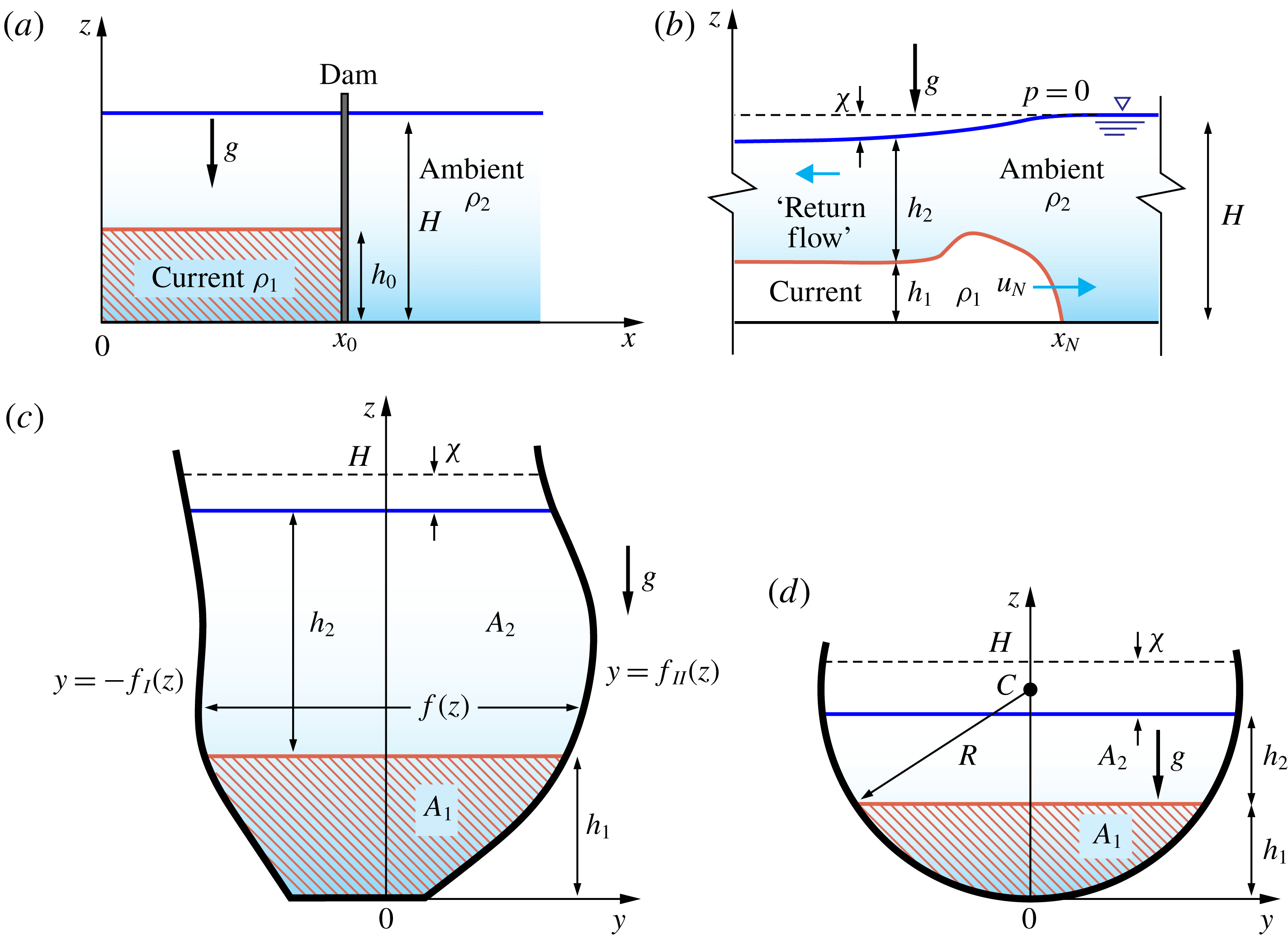
We consider a GC in a channel of circular cross-section open to the atmosphere (see figure 1). Here we use subscripts
 $1$
and
 $2$
to denote dense and less dense fluids. The density difference
 $\unicode[STIX]{x0394}\unicode[STIX]{x1D70C}=\unicode[STIX]{x1D70C}_{1}-\unicode[STIX]{x1D70C}_{2}$
is positive, but not necessarily small, which means that we consider both Boussinesq and non-Boussinesq systems. The bottom is at
 $z=0$
and the open surface is at
 $z={\hat{H}}$
. Initially, at time
 $t=0$
, the open surface of the fluids is horizontal at
 ${\hat{H}}=H=\text{const.}$
The open surface implies that (i) the total height is a function of
 $x,t$
and (ii) the pressure at the top is a given constant, conveniently set to
 $0$
. We write
 $$\begin{eqnarray}h_{1}(x,t)+h_{2}(x,t)={\hat{H}}(x,t);\quad p_{2}(z={\hat{H}})=0,\end{eqnarray}$$
where
 $h_{i}$
is the thickness of the layer and
 $p_{i}$
the pressure of fluid
 $i$
. It is also convenient to define the depression of the interface from the initial height
 $$\begin{eqnarray}\unicode[STIX]{x1D712}(x,t)=H-{\hat{H}}(x,t).\end{eqnarray}$$
These conditions are in contrast to the fixed-top channel case, and the source of the differences between the formulations. The open-surface case is in general more difficult for analysis and interpretation. This will be elucidated below. However, there are significant and useful similarities between the resulting GCs, and hence it makes sense to follow the methodology used for the fixed-top analysis, with due modification (Ungarish Reference Ungarish2018).
We present briefly the formulation for a general cross-sectional area defined by the width function
 $f(z)$
(see figure 1). We keep in mind that the present work is an implementation for the special case of a section of a circle, as specified later.
Gravity current with the top of the free surface open to a constant pressure. (a) Side-view geometry before lock release and (b) after lock release, with the dense current advancing in the channel. (c) Scheme for a cross-section of generic shape and (d) for a semicircular cross-section.
The pertinent areas are
 $$\begin{eqnarray}A_{1}=\int _{0}^{h_{1}}f(z)\,\text{d}z,\quad A_{2}=\int _{h_{1}}^{{\hat{H}}}f(z)\,\text{d}z,\quad A_{T}=A_{1}+A_{2}.\end{eqnarray}$$
The total area
 $A_{T}$
is a function of
 $x,t$
, and we denote by
 $A_{T}(0)$
the value at
 $t=0$
when
 ${\hat{H}}=H$
. Note that, using Leibniz’s formula, we obtain
 $$\begin{eqnarray}\frac{\unicode[STIX]{x2202}A_{1}}{\unicode[STIX]{x2202}t}=f(h_{1})\frac{\unicode[STIX]{x2202}h_{1}}{\unicode[STIX]{x2202}x};\quad \frac{\unicode[STIX]{x2202}A_{2}}{\unicode[STIX]{x2202}t}=f({\hat{H}})\frac{\unicode[STIX]{x2202}{\hat{H}}}{\unicode[STIX]{x2202}t}-f(h_{1})\frac{\unicode[STIX]{x2202}h_{1}}{\unicode[STIX]{x2202}t};\quad \frac{\unicode[STIX]{x2202}A_{T}}{\unicode[STIX]{x2202}t}=f({\hat{H}})\frac{\unicode[STIX]{x2202}{\hat{H}}}{\unicode[STIX]{x2202}t},\end{eqnarray}$$
and similarly for derivatives with respect to
 $x$
.
The thin-layer or shallow-water (SW) approximation used here is an extension of the derivation for the fixed-top (and free-slip) two-layer system with a general cross-section; see Ungarish (Reference Ungarish2018). Briefly, because the layers are thin (
 $h_{0}\ll x_{0}$
), the
 $x$
-motion and acceleration are dominant, and hence (i) the local pressure
 $z$
-balance is hydrostatic, with pressure continuity at the interface
 $z=h_{1}$
; and (ii) the motion can be represented by the averaged (over the local
 $A_{i}$
) velocities
 $\bar{u}_{i}(x,t)$
,
 $i=1,2$
. Since the Reynolds number is large, the viscous terms are negligible (except for some dissipation in jumps) and the
 $x$
-momentum equations can be expressed by a simplified balance between averaged inertial terms and hydrostatic pressure gradient (
 $x$
-component). The pressure-driving term is dominated by the
 $\unicode[STIX]{x0394}\unicode[STIX]{x1D70C}\,g$
effect, and is also referred to as the buoyancy-driving effect. The result of this manipulation yields a system for the variables
 $h_{1},h_{2},\bar{u}_{1},\bar{u}_{2}$
as functions of
 $x$
and
 $t$
. Keeping in mind that the areas
 $A_{1},A_{2}$
are unique functions of
 $h_{1},h_{2}$
, it is sometimes convenient to interchange between these variables in the formulation.
For simplicity of notation we drop the overbar that denotes the averaged velocity. We obtain the following results.
The continuity equations, expressing the volume balance of incompressible non-mixing streams of fluids, read
 $$\begin{eqnarray}\frac{\displaystyle \unicode[STIX]{x2202}A_{i}}{\displaystyle \unicode[STIX]{x2202}t}+\frac{\displaystyle \unicode[STIX]{x2202}u_{i}A_{i}}{\displaystyle \unicode[STIX]{x2202}x}=0\quad (i=1,2).\end{eqnarray}$$
Both fluids are in
 $z$
-hydrostatic balance
 $\unicode[STIX]{x2202}p_{i}/\unicode[STIX]{x2202}z=\unicode[STIX]{x1D70C}_{i}g$
, and the pressure is continuous at the interface
 $z=h_{1}$
(except for the segments of vertical jumps). Subject to the open-surface condition
 $p_{2}(z={\hat{H}})=0$
, this yields
 $$\begin{eqnarray}p_{1}=\unicode[STIX]{x1D70C}_{2}gh_{2}+\unicode[STIX]{x1D70C}_{1}g(h_{1}-z);\quad p_{2}=\unicode[STIX]{x1D70C}_{2}g({\hat{H}}-z),\end{eqnarray}$$
and hence the driving pressure effect is
 $$\begin{eqnarray}\frac{\displaystyle \unicode[STIX]{x2202}p_{1}}{\displaystyle \unicode[STIX]{x2202}x}=\unicode[STIX]{x1D70C}_{2}g\frac{\displaystyle \unicode[STIX]{x2202}{\hat{H}}}{\displaystyle \unicode[STIX]{x2202}x}+\unicode[STIX]{x0394}\unicode[STIX]{x1D70C}\,g\frac{\displaystyle \unicode[STIX]{x2202}h_{1}}{\displaystyle \unicode[STIX]{x2202}x};\quad \frac{\displaystyle \unicode[STIX]{x2202}p_{2}}{\displaystyle \unicode[STIX]{x2202}x}=\unicode[STIX]{x1D70C}_{2}g\frac{\displaystyle \unicode[STIX]{x2202}{\hat{H}}}{\displaystyle \unicode[STIX]{x2202}x}.\end{eqnarray}$$
In the basic
 $x$
-momentum equations for fluid with constant densities
 $\unicode[STIX]{x1D70C}_{1}$
and
 $\unicode[STIX]{x1D70C}_{2}$
we replace the pressure terms with (2.7), neglect the viscous terms and integrate the balance over the cross-sectional area of the corresponding fluid, taking into account the continuity equation. We obtain the momentum equations for the averaged variables
 $$\begin{eqnarray}\frac{\displaystyle \unicode[STIX]{x2202}u_{1}}{\displaystyle \unicode[STIX]{x2202}t}+u_{1}\frac{\displaystyle \unicode[STIX]{x2202}u_{1}}{\displaystyle \unicode[STIX]{x2202}x}=-\frac{\unicode[STIX]{x1D70C}_{2}}{\unicode[STIX]{x1D70C}_{1}}\left(g\frac{\displaystyle \unicode[STIX]{x2202}{\hat{H}}}{\displaystyle \unicode[STIX]{x2202}x}+\frac{\unicode[STIX]{x0394}\unicode[STIX]{x1D70C}}{\unicode[STIX]{x1D70C}_{2}}g\frac{\displaystyle \unicode[STIX]{x2202}h_{1}}{\displaystyle \unicode[STIX]{x2202}x}\right);\quad \frac{\displaystyle \unicode[STIX]{x2202}u_{2}}{\displaystyle \unicode[STIX]{x2202}t}+u_{2}\frac{\displaystyle \unicode[STIX]{x2202}u_{2}}{\displaystyle \unicode[STIX]{x2202}x}=-g\frac{\displaystyle \unicode[STIX]{x2202}{\hat{H}}}{\displaystyle \unicode[STIX]{x2202}x}.\end{eqnarray}$$
Unlike the fixed-top case, the system (2.5) and (2.8) is not amenable to further significant reduction. The firm connection
 $A_{1}u_{1}+A_{2}u_{2}=0$
of the former case has been replaced by the more flexible
 $p_{2}(z={\hat{H}})=0$
condition in the present system. A significant difficulty is that both
 $g$
and
 $g^{\prime }=(\unicode[STIX]{x0394}\unicode[STIX]{x1D70C}/\unicode[STIX]{x1D70C}_{2})g$
appear in the present momentum equations.
It is useful to cast the formulation in dimensionless standard form. Let
 $\unicode[STIX]{x1D700}=\unicode[STIX]{x1D70C}_{1}/\unicode[STIX]{x1D70C}_{2}-1$
, and
 $g^{\prime }=\unicode[STIX]{x1D700}g$
is the reduced gravity. We introduce the dimensionless variables by scaling
 $x$
with
 $x_{0}$
of the lock, while the vertical
 $z$
and lateral
 $y$
lengths are scaled with
 $h_{0}$
of the lock. The velocity is scaled with
 $U=(g^{\prime }h_{0})^{1/2}$
, and the time with
 $x_{0}/U$
. The subsequent variables are in dimensionless form, without any special notation, unless stated otherwise. In particular,
 $H$
is the height ratio of the unperturbed ambient to the lock. We also introduce the formal Reynolds number
 $Re_{0}=Uh_{0}/\unicode[STIX]{x1D708}$
, where
 $\unicode[STIX]{x1D708}$
is the kinematic viscosity of the dense fluid (the current). After some manipulation of continuity equations, we obtain a standard hyperbolic system for the variables
 $h_{1},u_{1},{\hat{H}},u_{2}$
; see (A 6). Even for the simple dam-break problem the analytical solution of this system is a formidable task, and hence we attempt numerical solutions.
For a numerical (finite difference) solution, it is convenient to cast the equations in conservation form. We introduce the variables
 $$\begin{eqnarray}q_{1}=A_{1}u_{1};\quad q_{2}=A_{2}u_{2};\quad \unicode[STIX]{x1D719}=[A_{1}+A_{2}-A_{T}(0)]/\unicode[STIX]{x1D700},\end{eqnarray}$$
where
 $A_{T}(0)$
is the area of the unperturbed ambient. Starting with (2.5) and (2.7) (in dimensionless form), and using (2.4), we obtain after some algebra
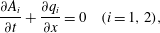 $$\begin{eqnarray}\displaystyle & \displaystyle \frac{\unicode[STIX]{x2202}A_{i}}{\unicode[STIX]{x2202}t}+\frac{\unicode[STIX]{x2202}q_{i}}{\unicode[STIX]{x2202}x}=0\quad (i=1,2), & \displaystyle\end{eqnarray}$$
 $$\begin{eqnarray}\displaystyle & \displaystyle \frac{\unicode[STIX]{x2202}q_{1}}{\unicode[STIX]{x2202}t}+\frac{\unicode[STIX]{x2202}}{\unicode[STIX]{x2202}x}\left[\frac{q_{1}^{2}}{A_{1}}+{\displaystyle \frac{1}{2(1+\unicode[STIX]{x1D700})}}\frac{A_{1}^{2}}{f(h_{1})}\right]=-{\displaystyle \frac{1}{(1+\unicode[STIX]{x1D700})}}\frac{A_{1}}{f({\hat{H}})}\frac{\unicode[STIX]{x2202}\unicode[STIX]{x1D719}}{\unicode[STIX]{x2202}x}-{\displaystyle \frac{1}{2(1+\unicode[STIX]{x1D700})}}\frac{f^{\prime }(h_{1})A_{1}^{2}}{[f(h_{1})]^{3}}\frac{\unicode[STIX]{x2202}A_{1}}{\unicode[STIX]{x2202}x}, & \displaystyle \nonumber\\ \displaystyle & & \displaystyle\end{eqnarray}$$
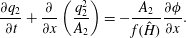 $$\begin{eqnarray}\displaystyle & \displaystyle \frac{\unicode[STIX]{x2202}q_{2}}{\unicode[STIX]{x2202}t}+\frac{\unicode[STIX]{x2202}}{\unicode[STIX]{x2202}x}\left(\frac{q_{2}^{2}}{A_{2}}\right)=-\frac{A_{2}}{f({\hat{H}})}\frac{\unicode[STIX]{x2202}\unicode[STIX]{x1D719}}{\unicode[STIX]{x2202}x}. & \displaystyle\end{eqnarray}$$
The variable
 $\unicode[STIX]{x1D719}$
represents the pressure influence in the ambient fluid due to the displacement of upper surface from the initial position; the scaling with
 $\unicode[STIX]{x1D700}$
renders this variable of the order of unity for both small and non-small values of
 $\unicode[STIX]{x1D700}$
, and this is advantageous for the accuracy of the numerical discretization error.
These equations are subject to initial and boundary conditions. At
 $t=0$
, fluids are at rest (
 $q_{1}=q_{2}=0$
) with given values of
 $h_{1},h_{2}$
(or
 $A_{1},A_{2}$
) in the lock
 $x\in [0,1]$
. The back wall at
 $x=0$
prevents motion and hence
 $q_{1}=q_{2}=0$
there for
 $t>0$
. The front (or nose)
 $x=x_{N}(t)$
of the current is a discontinuity, denoted by subscript
 $N$
. Here we apply the jump conditions derived in Ungarish (Reference Ungarish2019):
 $$\begin{eqnarray}\frac{\text{d}x_{N}}{\text{d}t}=u_{1N}=h_{1N}^{1/2}Fr;\quad h_{1N}+h_{2N}=H-\unicode[STIX]{x1D700}h_{1N}\left(1-\frac{1}{2}Fr^{2}\right).\end{eqnarray}$$
Here
 $Fr$
is of the order of unity, but the exact value depends on the geometry and
 $\unicode[STIX]{x1D700}$
, and is subject to energy and critical-speed restrictions. Note that in the Boussinesq limit
 $\unicode[STIX]{x1D700}\rightarrow 0$
, equation (2.13) recovers the fixed-top case: there is no depression of the interface. The details are given in Ungarish (Reference Ungarish2019), and briefly summarized in appendix A for the convenience of the reader.
The free input parameters for this system are: the density ratio
 $r=\unicode[STIX]{x1D70C}_{2}/\unicode[STIX]{x1D70C}_{1}$
(or
 $\unicode[STIX]{x1D700}=1/r-1$
); the height ratio of the current in the lock to the ambient,
 $H$
; and the geometry of the cross-section, expressed by the width function
 $f(z)$
. The aspect ratio
 $h_{0}/x_{0}$
has been scaled out from the SW formulation.
Consider the rectangular cross-section case,
 $f(z)=W=$
const. In this geometry,
 $A_{1}=h_{1}W,A_{2}=h_{2}W$
,
 $\unicode[STIX]{x1D719}=W(h_{1}+h_{2}-H)/\unicode[STIX]{x1D700}$
, and the last term on the right-hand side of (2.11) vanishes. The present formulation then coincides with the problem investigated in Longo et al. (Reference Longo, Ungarish, Di Federico, Chiapponi and Petrolo2018). We therefore adopt for the present problem an extension of the finite-difference MacCormack code which worked well for that problem. In particular: (i) to facilitate the numerical solution, we introduce the coordinate transformation
 $\unicode[STIX]{x1D709}=x/x_{N}(t)$
(see Ungarish Reference Ungarish2009, § 2.3). Now the finite-difference solution is concerned with the fixed domain
 $\unicode[STIX]{x1D709}\in [0,1]$
, and we can use constant homogeneous intervals
 $\unicode[STIX]{x1D6FF}\unicode[STIX]{x1D709}$
, typically 200, while the time step is typically 5–10 times smaller; (ii) to dampen numerical spurious oscillations, we add artificial-diffusion terms of the form
 $b(\unicode[STIX]{x1D6FF}\unicode[STIX]{x1D709})^{2}v_{\unicode[STIX]{x1D709}\unicode[STIX]{x1D709}}$
, where
 $v$
is the variable of the equation and
 $b$
is a constant of order 1. The computer memory and run time for a typical case of study are insignificant.
In the present investigation the cross-section is a circular profile of width
 $f(z)=[z(1-\unicode[STIX]{x1D6FD}z/2)]^{1/2}z\in [0,H]$
. Here
 $\unicode[STIX]{x1D6FD}=H/R\leqslant 2$
is the ratio of the height of the ambient to the radius of the circle. In our work, we consider the values of 1.5 and 1. Note that we can multiply
 $f(z)$
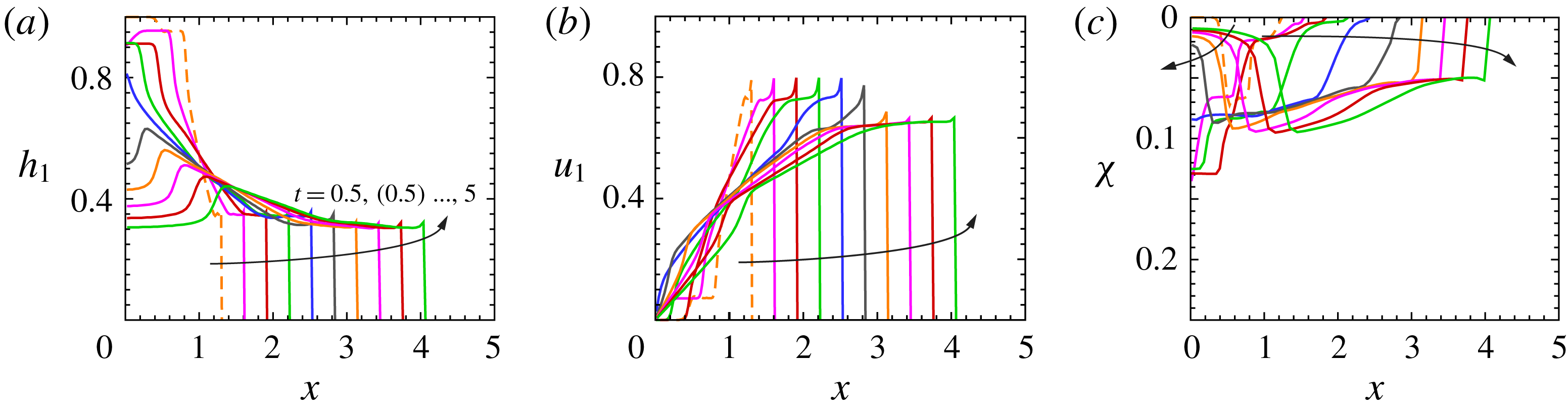
by an arbitrary positive constant without changing the problem and the results. Figures 2 and 3 display some typical SW solutions for the full-depth release with
 $r=0.586$
and for
 $\unicode[STIX]{x1D6FD}=1,H=1$
, corresponding to the laboratory experiment 5 (table 1), and the partial-depth release with
 $r=0.587$
and for
 $\unicode[STIX]{x1D6FD}=1,H=4/3$
, corresponding to the laboratory experiment 12.
Shallow-water results, simulation of experiment 5 (see table 1) with
 $r=0.586$
,
 $\unicode[STIX]{x1D6FD}=1$
,
 $H=1$
, full depth. (a) Thickness of the current, (b) average velocity of the current and (c) free-surface depression at
 $t=0.5,1,\ldots ,5$
with a time step equal to 0.5.
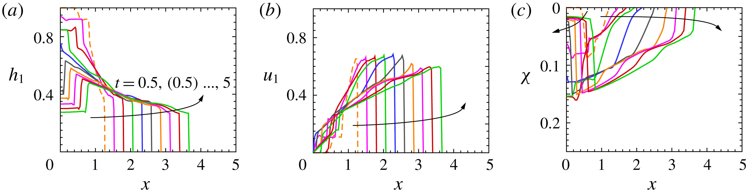
Shallow-water results, simulation of experiment 12 (see table 1) with
 $r=0.587$
,
 $\unicode[STIX]{x1D6FD}=1$
,
 $H=4/3$
, partial depth. (a) Thickness of the current, (b) average velocity of the current and (c) free-surface depression at
 $t=0.5,1,\ldots ,5$
with a time step equal to 0.5.
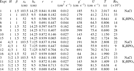
Parameters of the experiments in a circular channel of radius
 $R=9.5~\text{cm}$
, for
 $H=H^{\ast }/h_{0}$
,
 $\unicode[STIX]{x1D6FD}=H^{\ast }/R$
(with the superscript
 $^{\ast }$
indicating a dimensional variable),
 $Re_{0}=Uh_{0}/\unicode[STIX]{x1D708}$
, where
 $\unicode[STIX]{x1D708}$
is the kinematic viscosity of the current fluid. The last column indicates the chemical formula of salt added to obtain the current fluid.
As for the rectangular channel experiments (Longo et al.
Reference Longo, Ungarish, Di Federico, Chiapponi and Petrolo2018), there is a good correlation between
 $\unicode[STIX]{x1D712}$
and
 $h_{1}$
, with a more evident depression where the intruding current is thicker. This is a consequence of the larger values of the return flow in the ambient fluid where the denser fluid current is thicker, with a consequent large reduction of pressure manifested by the stronger depression. Similar SW solutions have been obtained also for the other systems listed in table 1. The salient results are reported later, in the context of comparisons with experiments.
3 The experimental layout and procedures
For a realistic observation of the flow field, and for the acquisition of reliable data for the validation of the theoretical models, we performed a series of experiments at the Hydraulic Laboratory of the University of Parma. A circular channel with internal radius of 9.5 cm and approximately 400 cm long, with walls in poly(methyl methacrylate), was used. Two different locks were employed, with a length of 52 and 103.5 cm respectively (see figure 4
a,b). The gate was a stainless steel plate in a guillotine arrangement, 0.1 cm thick, lowered by hand. The opening of the gate took approximately 0.4 s. A micro-switch closed by the gate was used to trigger the data acquisition for the sensors and also switched on a light-emitting diode initially in the field of view of the video camera used to record the position of the front of the current. The video camera, a Canon Legria HF 20 full HD (
 $1920~\text{pixel}\times 1080~\text{pixel}$
) at 25 frames per second, was used by an operator in order to follow the front of the GC as reflected by a mirror. A grid was attached to the tube and could be observed in the mirror in order to obtain the reference position of the advancing tip of the current. The resolution was better than
 $0.005~\text{cm}~\text{pixel}^{-1}$
; the overall uncertainty due to error in positioning the grid and to parallax distortion was less than 0.1 cm.
The layout of the experimental set-up. (a) The channel with the lock and four ultrasound distance meters; (b) the cross-section of the channel; (c) the guillotine gate. Distances are in centimetres.
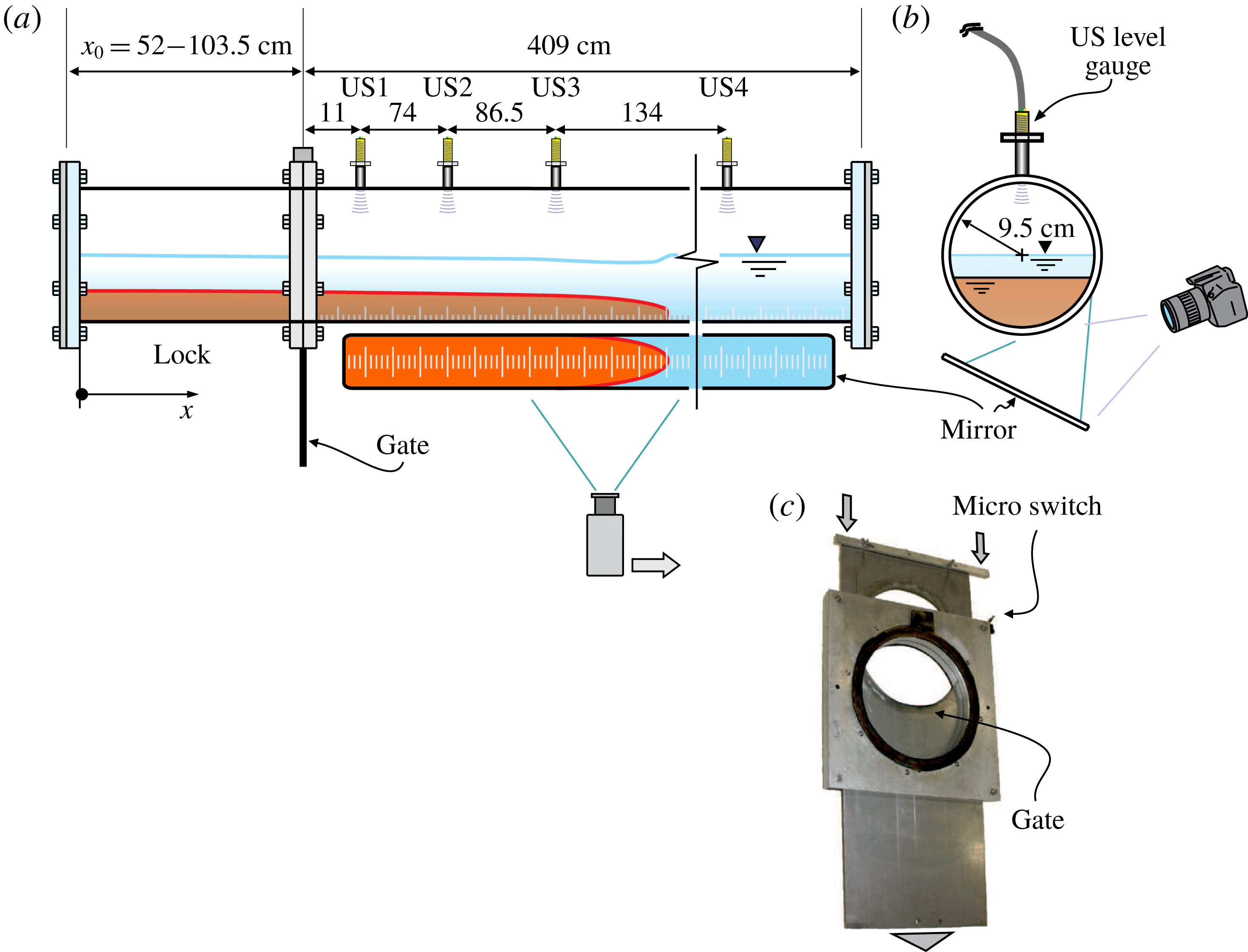
The measurement of the depression of the surface was a major challenge in our experiments. Four ultrasound distance meters (US1, US2, US3, US4) (TurckBanner Q45UR) were positioned on the top of the channel. Since the instruments have a blind zone of 5 cm, it was necessary to insert a circular guide to increase their distance from the free surface of the ambient fluid. The instruments have an accuracy of 0.03 cm and a data rate of 100 Hz. Occasionally, when the free surface breaks or is distorted by the waves with a strong curvature, the echo is lost and some spikes appear in the signal.
In a first series of experiments, sodium chloride (NaCl) was added to softened tap water in order to obtain high-density fluid (
 $\unicode[STIX]{x1D70C}\leqslant 1.200~\text{g}~\text{cm}^{-3}$
). To overcome the density limit of sodium chloride, dipotassium phosphate (
 $\text{K}_{2}\text{HPO}_{4}$
) was used, reaching a maximum density
 $\unicode[STIX]{x1D70C}\leqslant 1.710~\text{g}~\text{cm}^{-3}$
. Dipotassium phosphate is not toxic, can be easily bought since it is used in the food industry and it is much cheaper than other salts (e.g. sodium iodide) used to prepare high-density brines. We measured the values of the viscosity of the brines with a Ubbelohde viscometer, obtaining values one order of magnitude larger for high-density dipotassium phosphate-based brines with respect to sodium chloride-based brines. The Reynolds number is significantly reduced, but in all experiments it is high enough to ensure a non-viscous initial regime. Aniline dye was added in order to make visible the intruding current.
3.1 The uncertainty in variables and parameters
The variables and the parameters of the experiments are affected by an uncertainty which is estimated on the basis of the instrument characteristics and of the process of measurement. Mass density was measured by a densitometer with an accuracy of
 $10^{-3}~\text{g}~\text{cm}^{-3}$
, and hence the corresponding uncertainty for
 $r=\unicode[STIX]{x1D70C}_{2}/\unicode[STIX]{x1D70C}_{1}$
is
 $\unicode[STIX]{x0394}r/r\leqslant 0.2\,\%$
, with an uncertainty in the reduced gravity
 $g^{\prime }$
equal to 0.2 %. The level of the ambient fluid and of the intruding fluid in the lock was fixed with an accuracy of 0.1 cm and the relative uncertainty is
 $\unicode[STIX]{x0394}H/H\leqslant 1\,\%$
and
 $\unicode[STIX]{x0394}h_{0}/h_{0}\leqslant 1\,\%$
. The ratio
 $H/h_{0}$
is affected by an uncertainty at most equal to 2 %. The velocity scale had an uncertainty
 $\unicode[STIX]{x0394}U/U\leqslant 0.6\,\%$
and the time scale had an uncertainty equal to
 $\unicode[STIX]{x0394}T/T\leqslant 1.6\,\%$
. The Reynolds number had an uncertainty equal to
 $\unicode[STIX]{x0394}Re_{0}/Re_{0}\leqslant 2.6\,\%$
, also based on the assumption of an uncertainty of 1 % in estimating the kinematic viscosity. The free-surface level of the ambient fluid measured by the ultrasonic distance meters had an uncertainty of 0.03 cm.
4 The experiments
Sixteen experiments were performed, four with a long lock and twelve with a short lock. Note that
 $x_{0}/h_{0}$
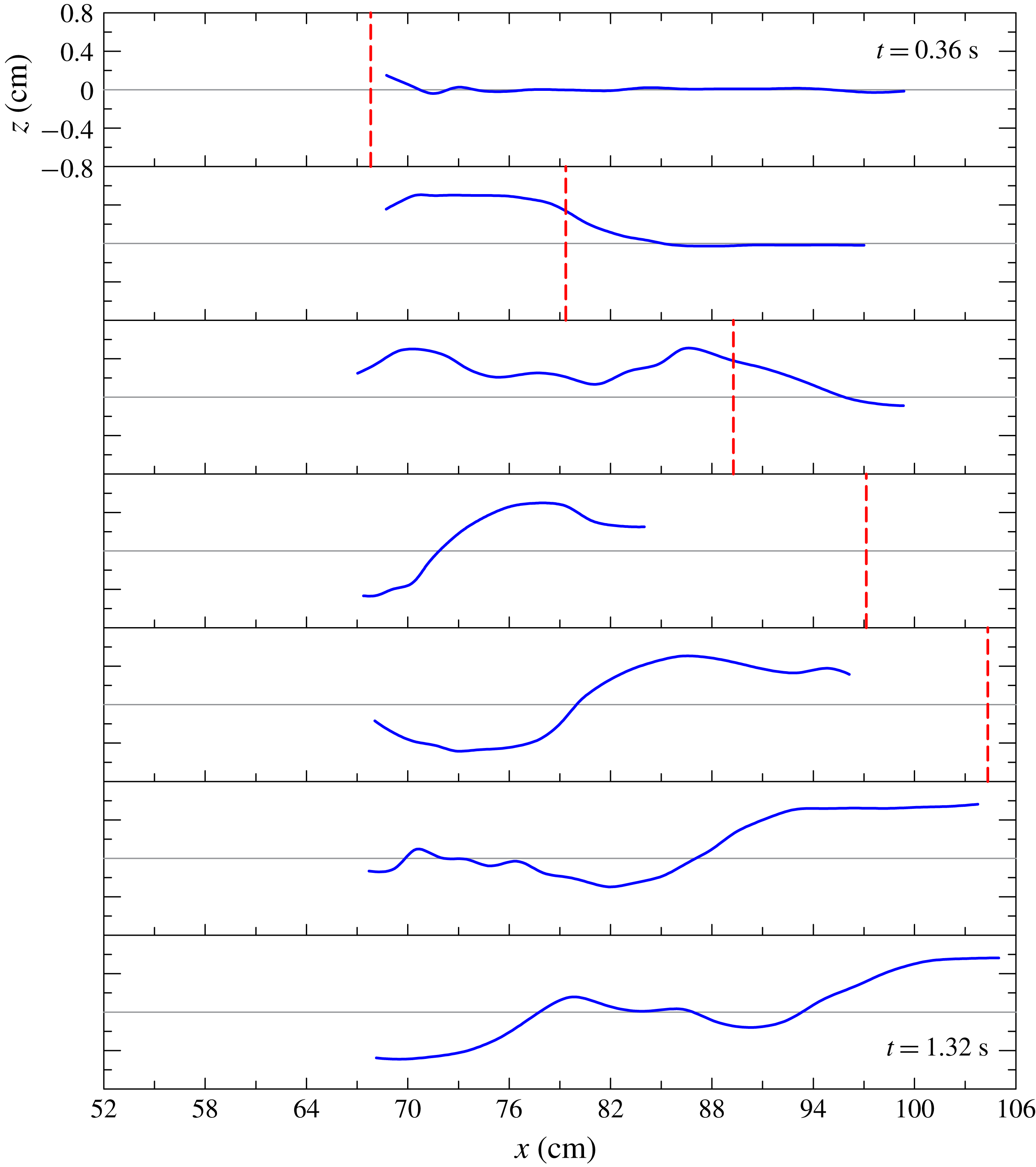
was larger than 3.6 in all experiments in accord with the thin-layer approximation of the SW model. Table 1 lists the main parameters for each experiment and figure 5 shows, for experiment 5, the advancement of the current in the domain near the lock through a series of snapshots; these show the formation of the depression behind the current nose. For a clearer view of the effect of the intruding current on the ambient fluid, figure 6 depicts the free-surface profiles for some snapshots of the same experiment. Some parts of the profiles are missing due to a limited contrast of the original frames.
A sequence of snapshots showing the free-surface shape near the lock, experiment 5. The dashed green horizontal line is the still water level. The time step between two snapshots is 0.4 s.
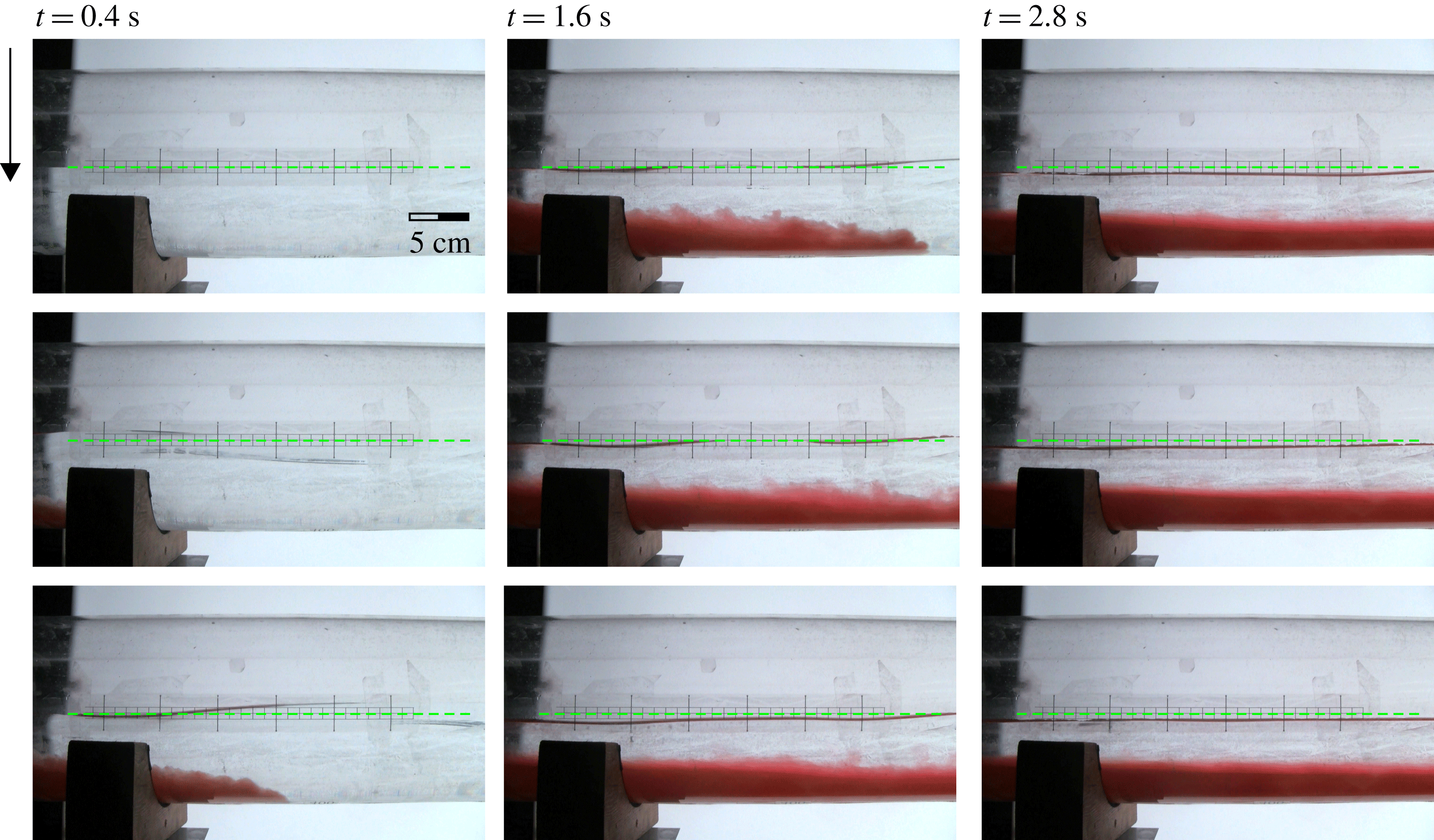
Free-surface profiles determined from the snapshots shown in figure 5. The red dashed line is the front position. The time step between two panels is 0.16 s.
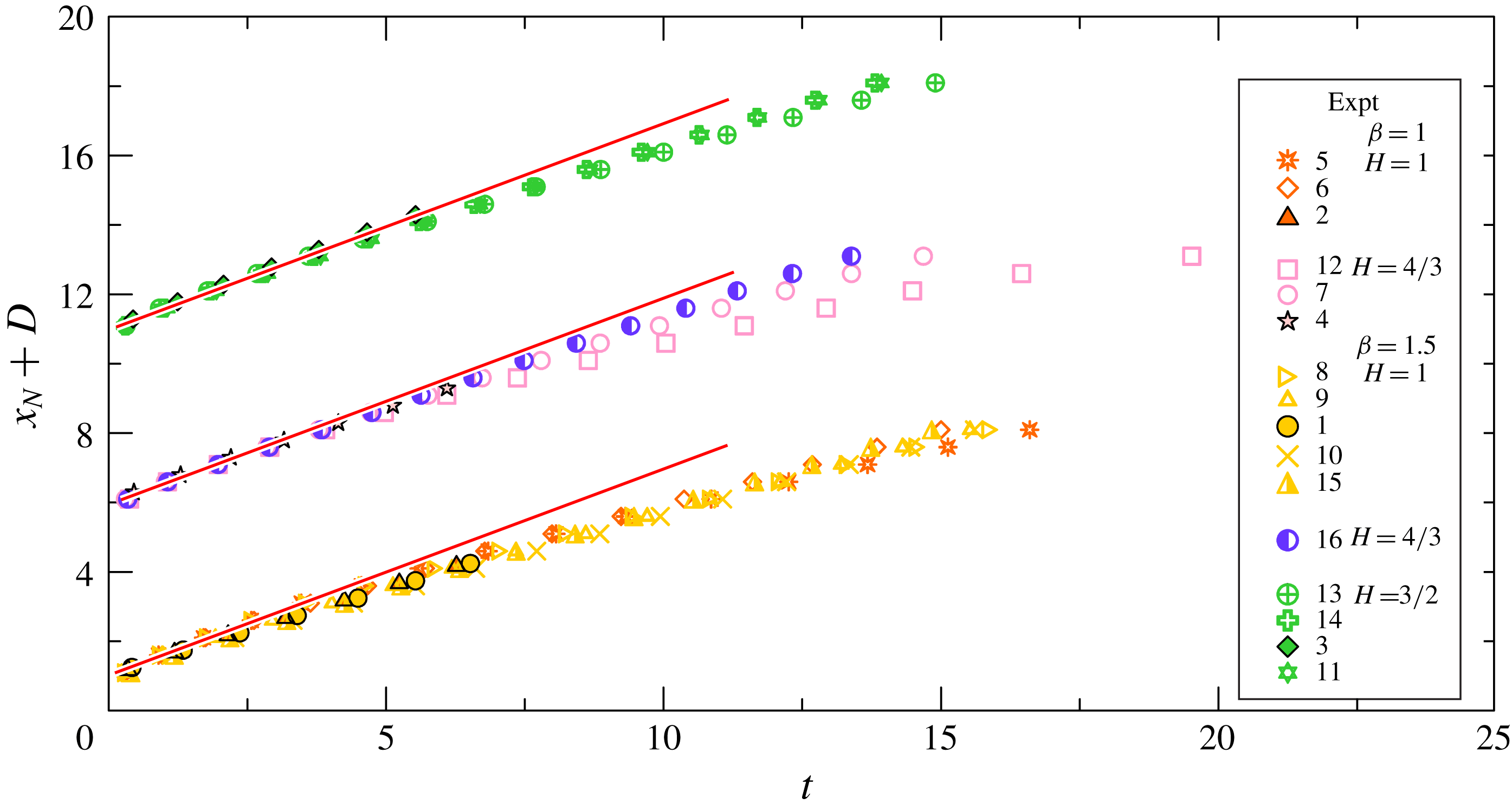
The front position expressed in dimensionless variables is shown in figure 7 for all the experiments. For ease of visualization, the symbols related to a group of experiments with similar parameters have been translated vertically and the experimental data have been re-sampled with a uniform space step. The SW simulations predict a slumping phase with almost constant
 $u_{N}$
until about
 $x_{N}=10$
(for a typical case, see figures 2
b and 3
b). In the experiments we detected a slight speed reduction starting at about
 $x_{N}=3{-}4$
, with the exception of the long-lock currents, whose propagation was limited by the length of the channel. This deviation from the SW prediction is attributed to viscous and perhaps entrainment effects which are not included in the theoretical model. Indeed, when comparing experiments 7, 12 and 16 (the mid-group in figure 7 with
 $H=4/3$
), the strongest deceleration is for experiment 12, which has the smallest value of
 $Re_{0}$
 $(3\times 10^{3})$
, while experiment 16 with the largest
 $Re_{0}$
 $(23\times 10^{3})$
displays fairly constant speed, and experiment 7, with
 $Re_{0}=9\times 10^{3}$
, is in between.
For experiments with low values of
 $r=\unicode[STIX]{x1D70C}_{2}/\unicode[STIX]{x1D70C}_{1}$
, an initial acceleration can be detected by observing the raw data (not shown), indicating that the inertia of the fluid initially counteracts gravity. Figure 8 shows a comparison between the theoretical and the experimental front speed
 $u_{N}$
, computed by fitting a line in the slumping phase. The theory always overestimates the experiments, with a difference below 30 %. The agreement is better for experiments with
 $\unicode[STIX]{x1D6FD}=1$
(circular cross-section half filled with ambient fluid) and with full-depth release. The experiments with
 $\unicode[STIX]{x1D6FD}=1.5$
generally show more disperse results. In particular, the full-depth release experiments show a modest reduction for increasing
 $r$
, a trend opposite to the theory. We notice that the free-surface waves developing in these experiments can significantly couple with the advancing GC, producing variable effects not included in the present model. In particular, the oscillatory motion induced by these waves can favour dissipation and generally modifies the return current in the ambient fluid; see also Stancanelli et al. (Reference Stancanelli, Musumeci and Foti2018) for details of these effects.
The propagation distance of the currents measured from the back wall in the lock for experiments with
 $H=1,4/3,3/2$
and
 $\unicode[STIX]{x1D6FD}=1,1.5$
. Filled symbols with black contour refer to long-lock experiments (1–4 with
 $x_{0}=103.5~\text{cm}$
); the other symbols refer to short-lock experiments (5–16 with
 $x_{0}=52~\text{cm}$
). One point in two is shown and data for experiments in partial depth have been translated in the vertical of
 $D=5$
units (
 $H=4/3$
) and
 $D=10$
units (
 $H=3/2$
) for ease of visualization. The straight lines indicate a constant speed of the front occurring during the slumping phase.
The comparison between theoretical (lines) and experimental (symbols) front speed. (a) Configuration with
 $\unicode[STIX]{x1D6FD}=1$
and
 $H=1$
(solid line and filled circles) and
 $H=4/3$
(dashed line and open circles); (b) configuration with
 $\unicode[STIX]{x1D6FD}=1.5$
and
 $H=1$
(solid line and filled circles),
 $H=4/3$
(dashed line and open circles) and
 $H=3/2$
(dash-dotted line and open triangles). The error bars indicate plus/minus one standard deviation.
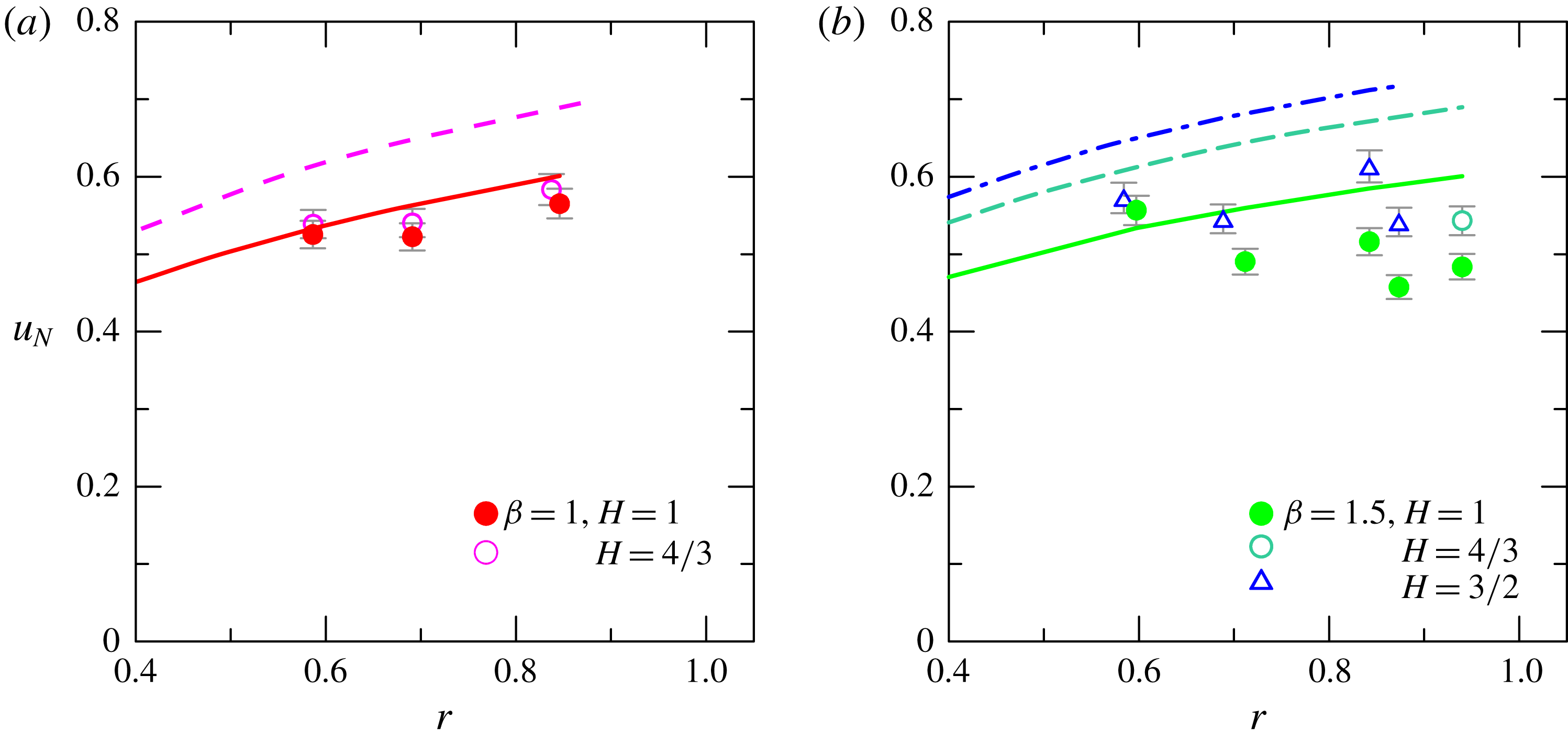
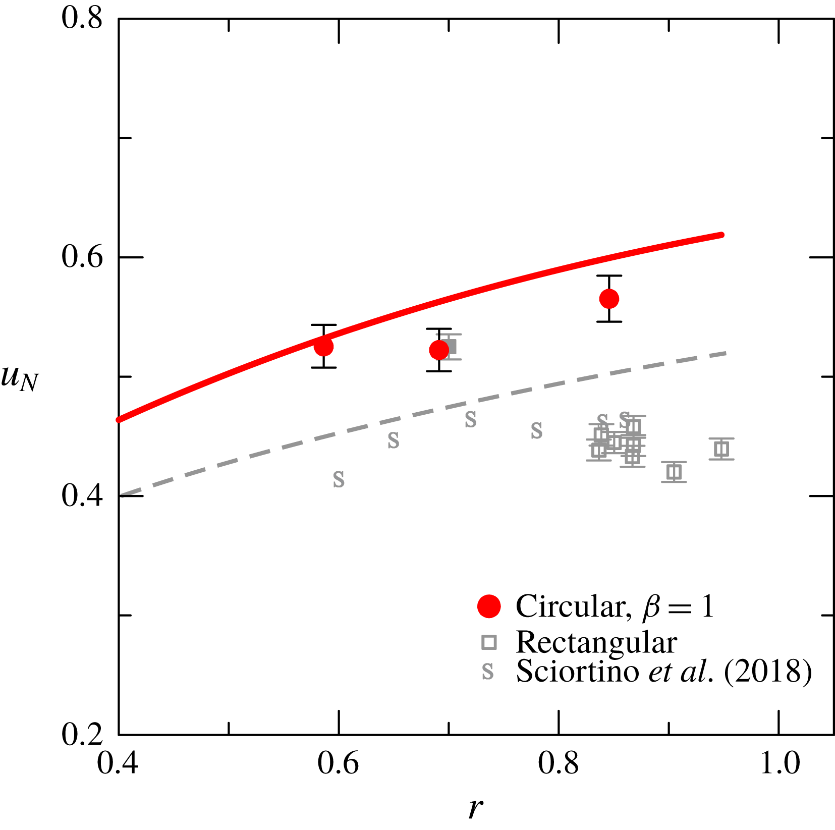
Figure 9 shows a comparison for the experiments in a rectangular cross-section (Longo et al.
Reference Longo, Ungarish, Di Federico, Chiapponi and Petrolo2018; Sciortino et al.
Reference Sciortino, Adduce and Lombardi2018) and the present experiments, in both cases for
 $H=1$
. Only experiments with
 $\unicode[STIX]{x1D6FD}=1$
are considered, since they represent a clear-cut expanding profile with
 $f^{\prime }(z)>0$
to contrast with the geometry with
 $f^{\prime }(z)=0$
of the rectangular cross-section (the other experiments with
 $\unicode[STIX]{x1D6FD}=1.5$
are characterized by a change of sign of
 $f^{\prime }(z)$
, which significantly influences the free-surface wave propagation – it is not a clear-cut comparison with the rectangular case). Both theory and experiments show higher front speed for the circular-cross-section channel. However, while for the rectangular case is evident a local maximum in the experimental data, with a maximum front speed (and a minimum discrepancy with theory) for
 $r\approx 0.7$
, for the circular case there is no clear evidence. Possibly some tests with
 $r<0.6$
could clarify the trend, but they are beyond the present experimental capabilities since it is extremely difficult to prepare fluids with mass density
 $\unicode[STIX]{x1D70C}\gg 1.700~\text{g}~\text{cm}^{-3}$
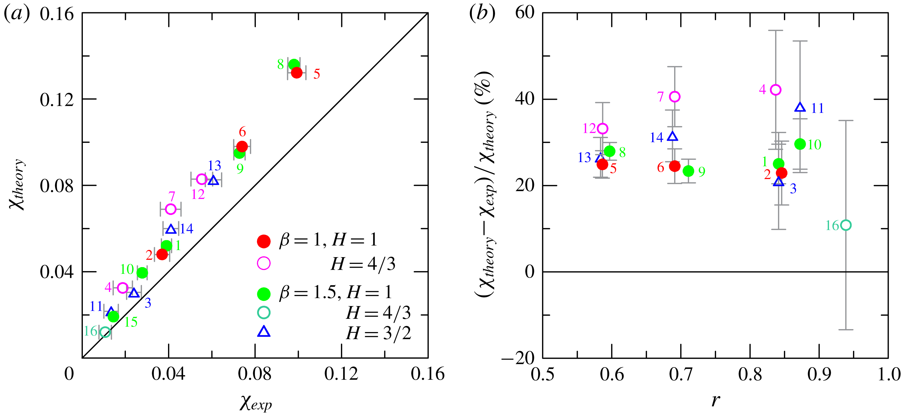
. Figure 10 shows a comparison between theory and experiments for the dimensionless depression, with the experimental depression computed as the average of the free-surface profile behind the nose of the current during the slumping phase. According to theory, this depression is proportional to
 $\unicode[STIX]{x1D700}$
: among the displayed points, the smallest depression is for experiment 16 (
 $\unicode[STIX]{x1D700}=0.07$
) and the largest is for experiment 8 (
 $\unicode[STIX]{x1D700}=0.68$
). As for the front speed, the experimental depression is systematically lower than the theoretical one, and for some experiments the difference is up to 40 %. A similar behaviour was also detected for experiments in a rectangular cross-section. Amongst the possible explanations there are (i) the presence of reflected free-surface waves which modulate the bound wave and limit the accuracy of the estimation of
 $\unicode[STIX]{x1D712}$
; (ii) the presence of billows which favour bursting, with coherent structures hitting the free surface; and (iii) the lower experimental front speed with respect to the theoretical one.
The comparison between theoretical (lines) and experimental (symbols) front speed for the present experiments,
 $\unicode[STIX]{x1D6FD}=1$
and
 $H=1$
, and experiments with a rectangular-cross-section channel described in Longo et al. (Reference Longo, Ungarish, Di Federico, Chiapponi and Petrolo2018) and in Sciortino et al. (Reference Sciortino, Adduce and Lombardi2018), again with
 $H=1$
. The error bars indicate plus/minus one standard deviation.
The comparison between theoretical and experimental free-surface depression in correspondence with the nose of the advancing current. (a) Theoretical versus experimental depression, where the line indicates perfect agreement; (b) relative error in depression estimation. The error bars indicate plus/minus one standard deviation.
The comparison between theoretical and experimental free-surface depression for experiment 5, full-depth lock release,
 $H=1$
,
 $\unicode[STIX]{x1D6FD}=1$
,
 $r=0.586$
. (a) Comparison at section where US1 is located,
 $x=11~\text{cm}$
from the gate; (b) comparison at section where US2 is located,
 $x=85~\text{cm}$
from the gate. The continuous grey and coloured curves are the measured and the filtered depressions, respectively; the dashed curves are the numerical results; the vertical dashed lines correspond to the time of arrival of the front of the current.
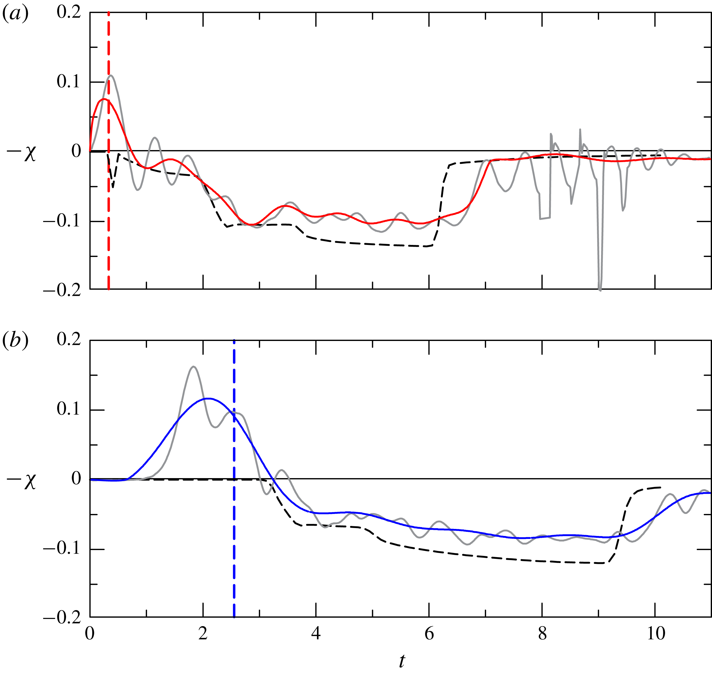
More details of the comparison between theory and experiments are given in figure 11, where the time series of the simulated and measured free-surface depression is shown at two different cross-sections. Figure 11(a) refers to the section at
 $x=11~\text{cm}$
from the gate. We first notice that a positive wave (bump) develops immediately after opening the gate (opening the gate with our guillotine gate means lowering the screen). Then a sequence of small-amplitude waves develop, and finally a dominant depression appears. The grey curves are the measured free-surface elevation and the coloured curves are the free-surface elevation low-pass filtered with a cut-off dimensionless frequency equal to 1, in order to eliminate the small-amplitude oscillations. A similar scenario is observed in figure 11(b), where the time series refer to a section at
 $x=85~\text{cm}$
from the gate. The experimental depression lags the front of the current, lasts longer and is overestimated by numerical simulations. The different duration is due to the discrepancy of the front speed of the current between theory and experiments (see figure 8), with experimental values always smaller than the numerical ones.
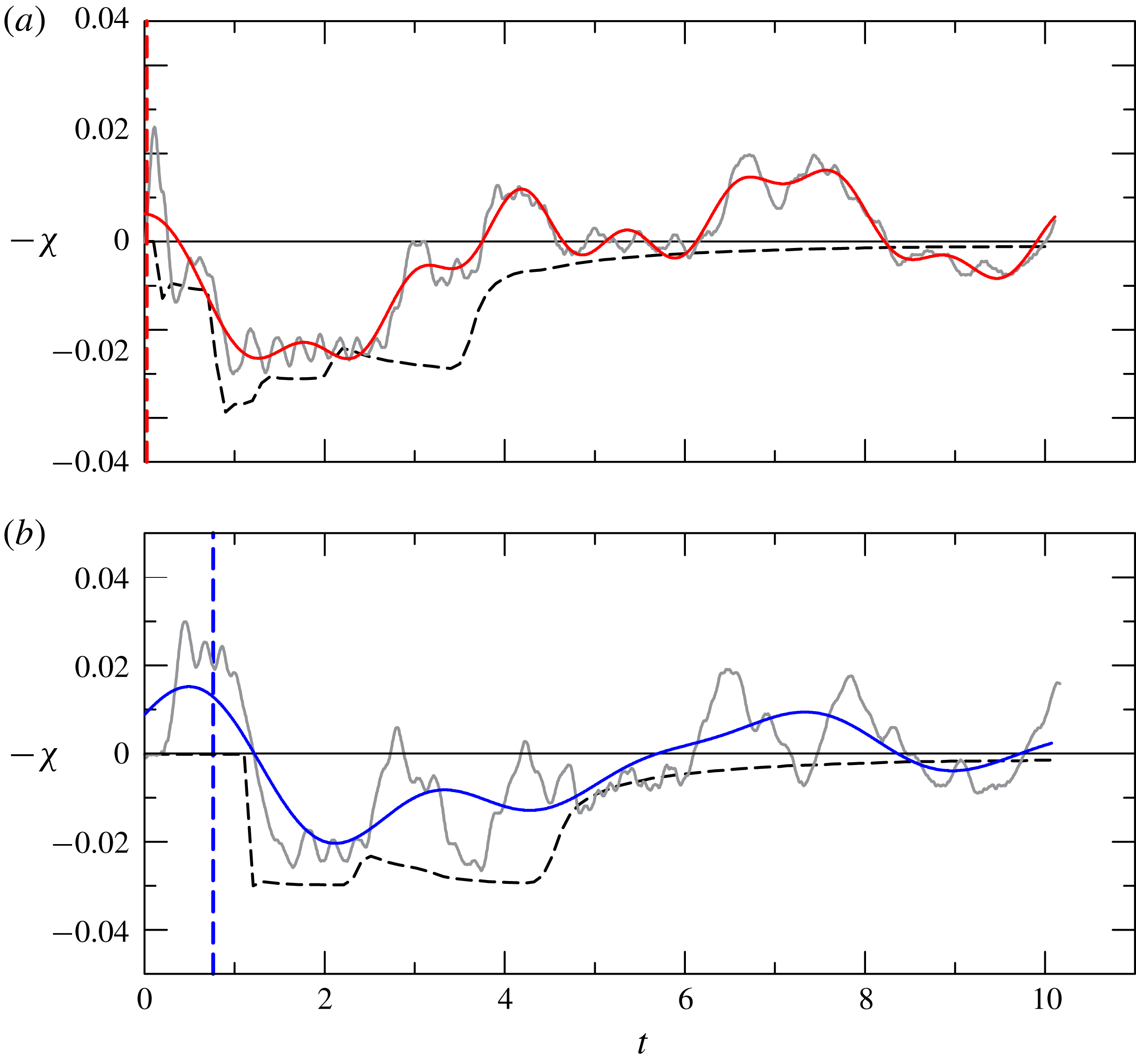
Similar results can be observed for a partial-depth lock release; these are shown in figure 12. The partial-depth case shows an experimental depression with a composite pattern of waves. We notice that the dimensional value of the depression is lower than for the full-depth lock release; hence perturbations and free-surface waves are more effective in modulating the depression.
The comparison between the theoretical and experimental free-surface depression for experiment 3, partial-depth lock release,
 $H=3/2$
,
 $\unicode[STIX]{x1D6FD}=1.5$
,
 $r=0.841$
. For description of the panels, see figure 11.
4.1 Free waves
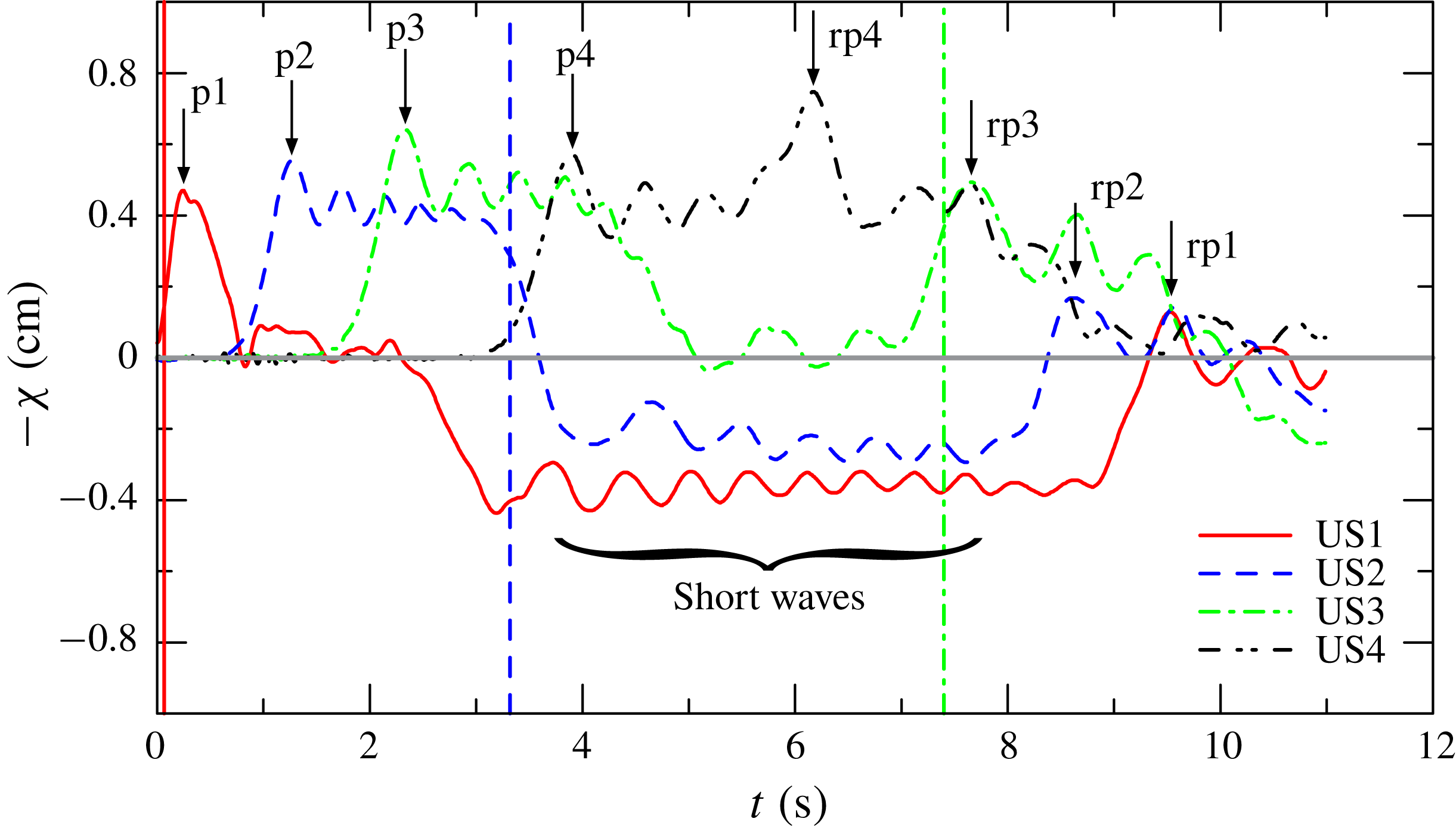
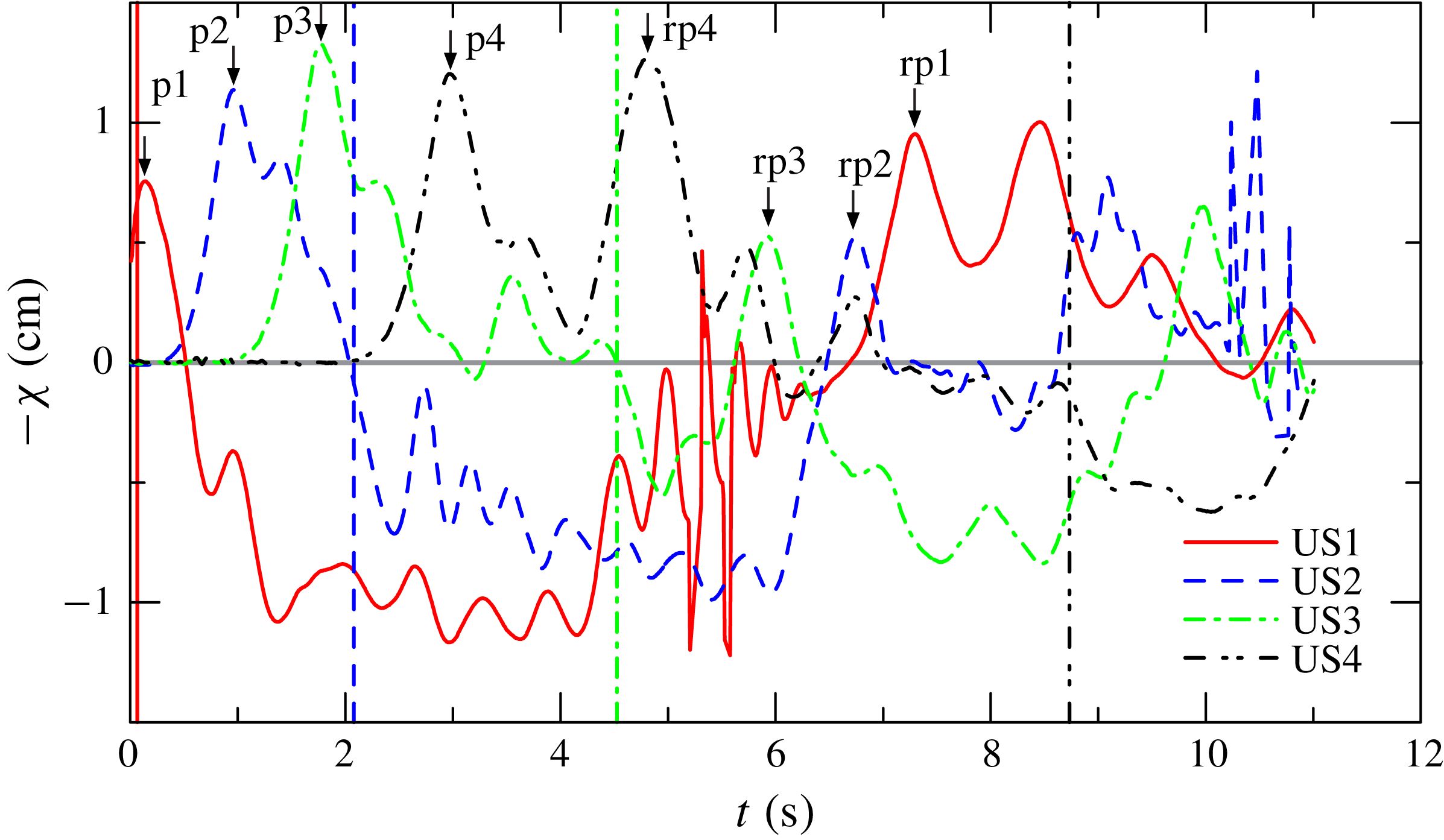
As for the rectangular cross-section, the depression of the free surface bound to the front of the current is preceded and followed by several free waves much faster than the current. A typical sequence of free-surface oscillations is shown in figure 13, with an initial solitary wave followed by the smaller-amplitude free-surface waves. The depression bound to the front of the current and recorded by the first ultrasound distance meter US1 is modulated only by the small-amplitude waves until the reflected solitary waves reach the section where the sensor US1 is located (
 $x=11~\text{cm}$
from the gate),
 ${\approx}10~\text{s}$
after the opening of the gate. The depression recorded by the second sensor US2 is delayed with respect to that recorded by US1 and is erased by the reflected waves after
 ${\approx}8.7~\text{s}$
. Due to reflections, the signals from sensors US3 and US4 are useless for measuring the bound wave, since they are affected by reflection before the arrival of the front of the current; nevertheless, they are useful for calculating the celerity of the free surface, for monitoring the channel performance and for properly measuring the time interval unaffected by reflections.
Free-surface displacement recorded by the ultrasound distance meters US1–US4 for experiment 2,
 $H=1$
,
 $\unicode[STIX]{x1D6FD}=1$
,
 $r=0.846$
. The vertical lines indicate the time of arrival of the front of the current in the sections where the distance meters are located, and the arrows indicate the initial peak (p1–4) and the reflected peak (rp1–4). The vertical line for US4 is out of the diagram.
Free-surface displacement recorded by the ultrasound distance meters for experiment 9,
 $H=1$
,
 $\unicode[STIX]{x1D6FD}=1.5$
,
 $r=0.711$
. For description, see figure 13.
In order to analyse the nature of these free-surface waves, let us consider (A 7) which relates the eigenvalues of the hyperbolic system describing the flow motion. In the domain where
 $u_{1}=u_{2}=0$
the equation reads
 $$\begin{eqnarray}\unicode[STIX]{x1D700}\unicode[STIX]{x1D706}^{4}-\left[\,\frac{\displaystyle A_{2}}{\displaystyle f({\hat{H}})}+\unicode[STIX]{x1D700}r\frac{\displaystyle A_{1}}{\displaystyle f(h_{1})}+r\frac{\displaystyle A_{1}}{\displaystyle f({\hat{H}})}\right]\unicode[STIX]{x1D706}^{2}+r\frac{\displaystyle A_{1}}{\displaystyle f(h_{1})}\frac{\displaystyle A_{2}}{\displaystyle f({\hat{H}})}=0,\end{eqnarray}$$
which for small
 $\unicode[STIX]{x1D700}$
yields the following solutions:
 $$\begin{eqnarray}\unicode[STIX]{x1D706}_{1.2}\approx \pm \sqrt{{\displaystyle \frac{A_{1}A_{2}}{f(h_{1})(A_{1}+A_{2})}}},\quad \unicode[STIX]{x1D706}_{3,4}\approx \pm \sqrt{{\displaystyle \frac{A_{1}+A_{2}}{\unicode[STIX]{x1D700}f({\hat{H}})}}}.\end{eqnarray}$$
The eigenvalues
 $\unicode[STIX]{x1D706}_{3,4}$
are ‘fast waves’ which in the unperturbed domain, where
 $h_{1}\rightarrow 0$
, are equal to
 $$\begin{eqnarray}\unicode[STIX]{x1D706}=\pm \sqrt{{\displaystyle \frac{A_{T}}{\unicode[STIX]{x1D700}f(H)}}},\end{eqnarray}$$
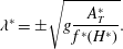
and, in dimensional form
 $$\begin{eqnarray}\unicode[STIX]{x1D706}^{\ast }=\pm \sqrt{g{\displaystyle \frac{A_{T}^{\ast }}{f^{\ast }(H^{\ast })}}}.\end{eqnarray}$$
Equation (4.4) represents also the celerity of perturbations (free-surface waves of infinitesimal height) travelling downstream and upstream in a channel with homogeneous fluid at rest, i.e. of long waves of infinitesimal amplitude (Lagrange celerity equation, see Chow Reference Chow1959). These perturbations are much faster than the characteristics controlling the GC and the front speed of the GC, and are independent of the density of the ambient fluid. The ratio
 $A_{T}^{\ast }/f^{\ast }(H^{\ast })\equiv \overline{H^{\ast }}$
is also defined as the hydraulic average depth, coincident with the local depth for a rectangular-cross-section channel (see equation (15) in Longo et al.
Reference Longo, Ungarish, Di Federico, Chiapponi and Petrolo2018).
For finite-amplitude perturbations, we can model the solitary wave in a homogeneous fluid in a circular channel with the following celerity (Peregrine Reference Peregrine1968; Teng & Wu Reference Teng and Wu1992):
 $$\begin{eqnarray}c^{\ast 2}=g\overline{H^{\ast }}\left[1+\left(1-{\displaystyle \frac{1}{3}}k^{2}b\overline{H^{\ast }}\right){\displaystyle \frac{\unicode[STIX]{x1D6FF}}{\overline{H^{\ast }}}}\right],\end{eqnarray}$$
where
 $\unicode[STIX]{x1D6FF}$
is the dimensional amplitude of the crest,
 $b=f^{\prime }(\overline{H^{\ast }})/f(\overline{H^{\ast }})$
and
 $k$
is a shape coefficient equal to 1.06 for a circular cross-section. Note that (4.4)–(4.5) are monotonically increasing with
 $\overline{H^{\ast }}$
(the latter if
 $b<0$
, equivalent to
 $\unicode[STIX]{x1D6FD}>1$
), hence higher values of
 $\overline{H^{\ast }}$
or increasing values of
 $\unicode[STIX]{x1D6FF}$
give faster propagating waves.
The experimental phase celerity can be estimated by observing the signal of the ultrasound probes. For the initial bump in experiment 2 the time delay of the initial peak (the peaks are indicated by arrows in figure 13 with symbols p1–4) between the sensors US1–US2, US2–US3 and US3–US4, respectively, gives an average celerity of
 $72\pm 0.5$
,
 $80\pm 0.5$
and
 $86\pm 0.5~\text{cm}~\text{s}^{-1}$
, compared to the theoretical celerity in (4.4) equal to
 $85.5\pm 0.5~\text{cm}~\text{s}^{-1}$
, and to
 $88\pm 1~\text{cm}~\text{s}^{-1}$
if it is computed according to the solitary wave celerity in (4.5). The second high peak for US4, indicated by rp4, is due to reflection at the end wall of the channel. The average celerity of the bump p4, propagating downstream and then upstream (the reflected component of p4 is rp4) is equal to
 $91\pm 0.5~\text{cm}~\text{s}^{-1}$
, again in good agreement with the theory. A similar analysis for the other reflected peaks cannot be performed since the sections where the sensors US1–US3 are located are reached by the intruding current before the arrival of the reflection, hence the reflected wave partly propagates in a domain where the return flow is present, and where the approximation giving (4.4) does not hold.
A similar analysis for experiment 9 gives
 $91\pm 1$
,
 $106\pm 1$
and
 $112\pm 1~\text{cm}~\text{s}^{-1}$
, with a theoretical celerity equal to
 $117.0\pm 0.8~\text{cm}~\text{s}^{-1}$
according to (4.4), or to
 $124.4\pm 1.5~\text{cm}~\text{s}^{-1}$
according to (4.5). Considering also p4 and rp4 (the peak due to reflection) yields an average celerity of
 $113\pm 1~\text{cm}~\text{s}^{-1}$
.
In both experiments there is a progressive acceleration of the initial bump, which far from the lock shows a celerity very close to the theoretical predictions. We also notice an increment of the crest amplitude from US1 to US3, followed by a small damping in the section of US4. In passing, the bump amplitude is of the same order as the depression. The bump is a long wave which interacts with the entire water column, hence we expect that the reflected bumps also interfere with the advancing dense current, reducing its front speed. In the present experiments we could not detect the reduction, which is presumably of the same order as the experimental fluctuations of the measurements.
A second family of free waves is represented by small-amplitude short-period waves (wave height of a few millimetres) in the tail of the initial bump, clearly visible when superimposed on the depression, indicated in figure 13 only for sensor US1. Their celerity is estimated by evaluating the time delay of the peak of the cross-correlation of the signals of two neighbour sensors. For experiment 2 the analysis yields an average celerity of
 $74\pm 0.5$
,
 $79\pm 0.5$
and
 $80\pm 0.5~\text{cm}~\text{s}^{-1}$
, quite similar to the values obtained for the initial bump. For experiment 9, the results are
 $75\pm 0.5$
,
 $107\pm 0.5$
and
 $113\pm 0.5~\text{cm}~\text{s}^{-1}$
, again similar to the celerity estimated for the bump.
We notice that there is a spatial evolution of these short waves, with a frequency reduction from US1 to US2 for experiment 2 (the frequency is hardly detectable from the signal of US3 and US4), and an increase for experiment 9. The frequency variation can be related to the fact that these short waves propagate on an unsteady current also with unsteady depths (see Haller & Tuba Özkan-Haller Reference Haller and Tuba Özkan-Haller2007); there is also the dispersivity due to higher order effects, as evident in (4.5). The wavelength of the waves is approximately 40 and 50 cm for the two different experiments. Since free (linear) gravity waves affect a water column depth equal to half their wavelength, we conclude that the short waves recorded in the present experiments propagate in the intermediate regime (they ‘feel’ the bottom) and interact with the entire flow domain underneath, including the dense fluid current advancing near the bottom of the channel. However, the effects of the interaction are weak since the wave height is quite low.
On a final note, it is worth mentioning that specific efforts were made to limit spurious disturbances caused by the experimental setting. First, the gate had a downward movement, thus avoiding falling drops during opening; moreover, the volume of the initial crest is less than
 $5~\text{cm}^{3}$
, substantially smaller than the volume of the lowered gate (nearly
 $13~\text{cm}^{3}$
); furthermore, the very limited volume of fluid dislocated by the lowered gate is not sufficient to transfer the energy contained in the observed waves. Other distinctive features of the oscillations in the trailing edge, like the period and the train evolution, exclude that the source of oscillation is the disturbance due to the gate. Finally, the channel length allowed enough time to collect data free from reflection effects.
5 Discussion and conclusions
We performed a combined theoretical and experimental study of lock-release inertial GCs. The systems under investigation are novel in several respects: non-Boussinesq, with open surface and in a long channel with semicircular cross-section (a prototype for the non-rectangular case). We used a novel SW formulation (including a very recent front condition, see Ungarish Reference Ungarish2019), and focused attention on the acquisition of data for the motion of the open-top surface (in addition to data for the motion of the current). We demonstrated that the propagation of the GC on the bottom produces a clear fingerprint on the upper surface, which can be evaluated by the simple SW model. We think that this provides a useful addition to the body of knowledge on the GC phenomena. We emphasize that the semicircular cross-section used here is just a particular test case, and the theory can be easily adapted to other cross-sections of interest like triangles and trapezoids.
The need to extend the available models for GCs to more complex situations than the simple one analysed by Benjamin has suggested this new set of experiments validated through a new formulation of the fundamental equations. The open top, the non-Boussinesq regime and the non-rectangular cross-section channel are conditions which require a two-layer SW model with proper modifications to include area-averaged variables. We demonstrated that the SW theory is able to solve such systems within the same approximation error as for the simpler system (Boussinesq, two-dimensional rectangular). The theory is self-contained (with no adjustable empirical coefficients), and the numerical solution of the SW system can be obtained in a short run time on simple computers. This is, in our opinion, of practical importance, because the other alternative for theoretical predictions, by Navier–Stokes numerical simulations, requires large memory and time resources for such systems. We showed that the geometry of the cross-section plays an important role; in particular, the propagation in a semicircle is faster than in a rectangle. This result is of practical relevance for the design of fluid-transport systems and in the interpretation of environmental flows.
The experiments were performed with
 $r$
ranging from
 $0.587$
to
 $0.939$
, with two different lock lengths, measuring the front speed and the free-surface depression in several sections. The analysis of the celerity of the free-surface waves indicates that these waves are not experimental artifacts, but are consistent with the theoretical model since they propagate according to the ‘fast’ eigenvalues of the hyperbolic system of equations. We notice that a similar result was obtained for the depression (a wave bound to the front of the current) measured in a rectangular channel (Longo et al.
Reference Longo, Ungarish, Di Federico, Chiapponi and Petrolo2018): if a top lid was present, the depression manifested itself as a pressure reduction in the ambient fluid, hence the presence/absence of the top lid simply changed the appearance of an intrinsic phenomenon. Specific conclusions of the present work are the following.
(i) The lock release of GCs advancing in a circular horizontal channel, with the top open to the atmosphere, shares many aspects with GCs propagating in rectangular-cross-section channels in similar conditions, with a depression of the interface between the ambient fluid and the atmosphere. The analytical model in its extended formulation is adequate for predicting the front speed of the intruding current and the surface depression, with the theoretical values systematically overestimating experiments, but with a fairly good agreement in a broad range of density ratios
 $r$
(0.584–0.939).
(ii) In addition to the depression, there are free waves propagating faster than the intruding current: an initial bump and short waves with small amplitude. Their celerity is well predicted by the model and equals two of the four eigenvalues (the ‘fast’ ones), at least in the part of the channel where the ambient fluid is still at rest. They are coincident with the free-surface waves of infinitesimal amplitude in an open channel flow. The analysis of the short waves suggests that they are modulated by the underneath flow field and interact with the advancing GC, even though the interaction is weak due to their low energy.
(iii) The overall agreement between theory and experiments is similar to that obtained for other GCs simulated with the SW model. The discrepancies are due partly to the accuracy limits of the experiments, and partly to the simplification of the model which completely neglects several phenomena affecting the flow motion, e.g. entrainment, dissipation, perturbations in the upstream ambient fluid and viscous effects (more evident at non-large Reynolds number). Indeed, the SW model is an averaged-velocity approximation of a very complicated flow-field system, and it is supposed to reproduce only the global behaviour of realistic flows. The advantage of a model as simple as possible is the absence of adjustable empirical parameters. We notice that a direct numerical simulation cannot be performed for the considered three-dimensional time-dependent non-Boussinesq GC, and that the available computational fluid dynamics codes introduce anyway some parameters for modelling turbulence and are extremely time consuming. In addition, their extensive application is not feasible even for a regular geometry like a circular channel.
(iv) This is the first paper concerning this complex problem, with the inclusion of numerous aspects in a holistic approach. Further investigations are required to disentangle the complexities.

The present work can be extended in several directions. First, similar studies for other geometries will be beneficial for enhancing confidence, and perhaps providing additional insights. Second, Navier–Stokes simulations can provide accurate diagnostic studies of the approximation errors of the SW model, and indicate possible improvements. Third, modifications of the SW model are formally possible by including friction and mixing/entrainment effects (La Rocca et al. Reference La Rocca, Adduce, Sciortino and Pinzon2008; Adduce, Sciortino & Proietti Reference Adduce, Sciortino and Proietti2011). The problem is that these effects depend on empirical coefficients which are unavailable for non-Boussinesq non-rectangular systems, and hence the theoretical work must be closely coupled with dedicated experiments/simulation. We hope that the present paper will motivate, and guide, the extensions in future work.
Appendix A. Calculation of
$Fr$
, characteristics and critical
$u_{N}$


The nose of the SW current is a discontinuity. We need a jump condition which relates the heights
 $h_{1,2}$
to speeds
 $u_{1,2}$
at the position
 $x=x_{N}$
.
We enclose this discontinuity by a thin-
 $x$
control volume and consider balances of volume, momentum and energy. The balance equations turn out to be as for a steady-state current, a case solved by Ungarish (Reference Ungarish2019). Suppose that
 $h_{1}$
is known. We obtain
 $$\begin{eqnarray}u_{1}=h_{1}^{1/2}Fr;\quad h_{2}=H-h_{1}-\unicode[STIX]{x1D712};\quad u_{2}=\left(1-\frac{A_{0}}{A_{2}}\right)u_{1}.\end{eqnarray}$$
Parameters
 $Fr$
and
 $\unicode[STIX]{x1D712}$
are calculated numerically from the following system:
 $$\begin{eqnarray}\unicode[STIX]{x1D712}=\unicode[STIX]{x1D700}h\left(1-{\textstyle \frac{1}{2}}Fr^{2}\right),\end{eqnarray}$$
 $$\begin{eqnarray}\left(\frac{A_{0}}{A_{2}}-1+\frac{A_{1}+A_{2}}{2A_{0}}\right)Fr^{2}=\frac{A_{2}}{A_{0}}+\frac{1}{\displaystyle \unicode[STIX]{x1D700}hA_{0}}\int _{H-\unicode[STIX]{x1D712}}^{H}(H-z)f(z)\,\text{d}z+\frac{1}{\displaystyle hA_{0}}\int _{0}^{h}zf(z)\,\text{d}z,\end{eqnarray}$$
where
 $h=h_{1}$
and
 $$\begin{eqnarray}A_{1}=\int _{0}^{h_{1}}f(z)\,\text{d}z;\quad A_{2}=\int _{h_{1}}^{H-\unicode[STIX]{x1D712}}f(z)\,\text{d}z;\quad A_{0}=A_{T}(0)=\int _{0}^{H}f(z)\,\text{d}z.\end{eqnarray}$$
The system is solved by iterations: guess
 $Fr$
, calculate
 $\unicode[STIX]{x1D712}$
by (A 2), correct
 $Fr$
by (A 3). A convenient starting point is
 $Fr=1$
. As shown in Ungarish (Reference Ungarish2019), solutions exist for
 $f(z)$
of interest, including the circular cross-section considered in this paper. However, the numerical evaluation of
 $Fr$
and
 $\unicode[STIX]{x1D712}$
(and actually of the pertinent GC) must be subjected to two constraints.
First, the energy dissipation of the jump domain must be non-negative. Balancing the in-flow and out-flow of the control volume, we can express this condition as
 $$\begin{eqnarray}Fr\leqslant \frac{A_{2}}{A_{0}}\sqrt{2}.\end{eqnarray}$$
This gives an upper limit to
 $h_{1N}$
.
A.1 Critical conditions
The second constraint accounts for the possibility of the fluid released from the lock staying attached to the jump. This can be expressed as a critical speed. The propagation cannot be with a larger, or supercritical, value.
We recall that the SW equations are a hyperbolic system of partial differential equations. The flow in the domain
 $0\leqslant x\leqslant x_{N}(t)$
is dominated by characteristics, and hence
 $\text{d}x_{N}/\text{d}t=u_{1}$
cannot exceed the speed of the corresponding characteristic; this is referred to as the subcritical flow condition.
The SW system of (2.5) and (2.8) can be rewritten for the variables
 $h_{1},u_{1},{\hat{H}},u_{2}$
as follows:
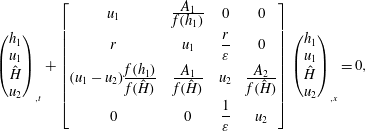 $$\begin{eqnarray}\left(\begin{array}{@{}c@{}}h_{1}\\ u_{1}\\ {\hat{H}}\\ u_{2}\end{array}\right)_{,t}+\left[\begin{array}{@{}cccc@{}}u_{1} & \frac{\displaystyle A_{1}}{\displaystyle f(h_{1})} & 0 & 0\\ r & u_{1} & {\displaystyle \frac{r}{\unicode[STIX]{x1D700}}} & 0\\ (u_{1}-u_{2})\frac{\displaystyle f(h_{1})}{\displaystyle f({\hat{H}})} & \frac{\displaystyle A_{1}}{\displaystyle f({\hat{H}})} & u_{2} & \frac{\displaystyle A_{2}}{\displaystyle f({\hat{H}})}\\ 0 & 0 & {\displaystyle \frac{1}{\unicode[STIX]{x1D700}}} & u_{2}\end{array}\right]\left(\begin{array}{@{}c@{}}h_{1}\\ u_{1}\\ {\hat{H}}\\ u_{2}\end{array}\right)_{,x}=0,\end{eqnarray}$$
where the comma indicates the partial derivative. The rearrangement requires some manipulation of the continuity equation for layer 2, and use of (2.4). Recall
 $r=(1+\unicode[STIX]{x1D700})^{-1}$
, and
 $h_{2}={\hat{H}}-h_{1}$
.
The characteristics are the eigenvalues
 $\unicode[STIX]{x1D706}_{i}$
of the matrix of coefficients, given by
 $$\begin{eqnarray}\displaystyle & & \displaystyle \unicode[STIX]{x1D700}(u_{1}-\unicode[STIX]{x1D706})^{2}(u_{2}-\unicode[STIX]{x1D706})^{2}-(u_{1}-\unicode[STIX]{x1D706})^{2}\frac{\displaystyle A_{2}}{\displaystyle f({\hat{H}})}-\unicode[STIX]{x1D700}r(u_{2}-\unicode[STIX]{x1D706})^{2}\frac{\displaystyle A_{1}}{\displaystyle f(h_{1})}\nonumber\\ \displaystyle & & \displaystyle \quad -\,r(u_{1}-\unicode[STIX]{x1D706})(u_{2}-\unicode[STIX]{x1D706})\frac{\displaystyle A_{1}}{\displaystyle f({\hat{H}})}+r(u_{1}-u_{2})(u_{2}-\unicode[STIX]{x1D706})\frac{\displaystyle A_{1}}{\displaystyle f(h_{1})}\frac{\displaystyle f(h_{1})}{\displaystyle f({\hat{H}})}+r\frac{\displaystyle A_{1}}{\displaystyle f(h_{1})}\frac{\displaystyle A_{2}}{\displaystyle f({\hat{H}})}=0.\nonumber\\ \displaystyle & & \displaystyle\end{eqnarray}$$
In general, the solution of these fourth-order equations is not insightful, except for the requirement that the roots are real. However, interestingly, the criterion for critical
 $Fr$
can be obtained. The condition
 $u_{1}=\unicode[STIX]{x1D706}$
reduces (A 7) to
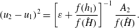 $$\begin{eqnarray}(u_{2}-u_{1})^{2}=\left[\unicode[STIX]{x1D700}+\frac{f(h_{1})}{f({\hat{H}})}\right]^{-1}\frac{A_{2}}{f({\hat{H}})}.\end{eqnarray}$$
We apply this condition to the nose jump of the GC where
 $u_{1}=Frh_{1}^{1/2}$
,
 ${\hat{H}}=H-\unicode[STIX]{x1D712}$
and
 $u_{2}-u_{1}=-(A_{0}/A_{2})u_{1}$
.
Then the critical condition yields
 $$\begin{eqnarray}Fr^{2}\frac{h_{1}}{H}=\frac{A_{2}^{3}}{A_{0}^{2}Hf(H-\unicode[STIX]{x1D712})}\left[\unicode[STIX]{x1D700}+\frac{f(h_{1})}{f(H-\unicode[STIX]{x1D712})}\right]^{-1}.\end{eqnarray}$$
This gives an upper limit to
 $h_{1}=h_{1N}$
.
In all tested cases, the critical-flow restriction was slightly more severe than the energy-dissipation limitation.



