





1. Introduction
Shock-wave–boundary-layer interactions (SWBLIs) represent a fundamental and challenging phenomenon in high-speed aerodynamics, commonly encountered in transonic wings, supersonic inlets and turbomachinery blades (Sabnis & Babinsky Reference Sabnis and Babinsky2023). In these practical configurations, SWBLIs induce complex flow features, including boundary-layer separation, unsteady shock motion and severe pressure and thermal loads. These effects further complicate the physical understanding of SWBLIs, and constitute a persistent bottleneck in aircraft design.
Systematic research on SWBLIs can be traced back to the 1940s, driven by the emergence of transonic flight and the development of capable wind tunnel facilities. Early foundational work combined experimental visualisation with theoretical modelling. Donaldson (Reference Donaldson1944), Liepmann (Reference Liepmann1946) and Ackeret et al. (Reference Ackeret, Feldmann and Rott1947) were among the first to experimentally document the key flow structures of SWBLIs. Building upon earlier ideas of Lighthill (Reference Lighthill1953), Gadd (Reference Gadd1957) and Chapman et al. (Reference Chapman, Kuehn and Larson1958), Stewartson & Williams (Reference Stewartson and Williams1969) established the comprehensive asymptotic theory of free interaction, which was confirmed by the detailed experimental measurements of Erdos & Pallone (Reference Erdos and Pallone1962). Subsequent contributions (Reyhner & Flügge-Lotz Reference Reyhner and Flügge-Lotz1968; Hankey & Holden Reference Hankey and Holden1975; Délery et al. Reference Délery, Marvin and Reshotko1986; Degrez et al. Reference Degrez, Boccadoro and Wendt1987; Stanewsky Reference Stanewsky1988) further shaped the general understanding of SWBLIs.
However, the aforementioned studies predominantly focused on the static or time-averaged characteristics of SWBLIs and therefore cannot fully explain certain dynamic phenomena in high-speed flights, such as transonic wing buffet and inlet buzz. Although SWBLI unsteadiness was reported as early as the 1950s (Chapman et al. Reference Chapman, Kuehn and Larson1958), progress on this topic was long hindered by the limited experimental measurement techniques (Dolling Reference Dolling2001). It was not until the early 1990s that the inherent unsteadiness in SWBLIs began to receive substantial attention. In the context of turbulent interactions, experiments across a variety of configurations consistently captured low-frequency motions, manifesting as shock-foot oscillation and periodic ‘breathing’ of the separation bubble (Erengil & Dolling Reference Erengil and Dolling1991; Brusniak & Dolling Reference Brusniak and Dolling1994; Dupont et al. Reference Dupont, Haddad and Debieve2006; Dussauge et al. Reference Dussauge, Dupont and Debiève2006). A defining signature of this unsteadiness is its dominant low-frequency content, typically one to two orders of magnitude lower than the characteristic turbulence frequencies in the incoming boundary layer. The origins of the unsteadiness are generally categorised into two types: upstream and downstream mechanisms. The upstream mechanism is associated with the interaction of large-scale structures in the upstream boundary layer (Ganapathisubramani et al. Reference Ganapathisubramani, Clemens and Dolling2007), while the downstream mechanism attributes the unsteadiness to the intrinsic dynamics of the recirculation bubble (Dussauge & Piponniau Reference Dussauge and Piponniau2008).
More recent research indicates that both the upstream and downstream mechanisms contribute to this unsteadiness, with their relative importance depending on the interaction strength and separation length. Clemens & Narayanaswamy (Reference Clemens and Narayanaswamy2014) noted that the two mechanisms appear to be closely linked to the scale of separation, with larger separation bubbles tending to strengthen the influence of the downstream mechanism. Nichols et al. (Reference Nichols, Larsson, Bernardini and Pirozzoli2017) employed both linear (global stability analysis, GSA) and nonlinear (dynamic mode decomposition) analyses of turbulent SWBLIs, and attributed the low-frequency motion to a damped, oscillatory intrinsic mode excited by upstream disturbances. Hao (Reference Hao2023) combined GSA and resolvent analysis, showing that the low-frequency unsteadiness arises from modal resonance between the leading global mode and external forcing. In transitional SWBLIs, Ben Hassan Saïdi et al. (Reference Ben Hassan Saïdi, Wang, Fournier, Tenaud and Robinet2025) proposed a triadic mechanism to explain the unsteadiness and the bubble ‘breathing’, which involves nonlinear saturation of the convective instabilities in the shear layer, and the upstream propagation of perturbations within the separation bubble. Mauriello et al. (Reference Mauriello, Sharma, Larchevêque and Sandham2025) imposed two oblique modes with closely spaced frequencies such that their difference fell within the low-frequency band of unsteadiness, and showed that the low-frequency unsteadiness can be generated by quadratic nonlinear interactions that produce a difference-frequency component between the two oblique waves.
In contrast to turbulent and transitional interactions, unsteadiness in laminar SWBLIs received much less attention, despite the practical significance and diverse underlying mechanisms. Laminar interactions can trigger boundary-layer transition (Kachanov Reference Kachanov1994) and thereby induce substantial changes in aerodynamic performance, including increased skin-friction drag and aero-heating loads. With the advancement of high-fidelity numerical simulations and linear stability theory (LST) (Malik Reference Malik1989; Zhong & Wang Reference Zhong and Wang2012) for high-Mach-number boundary layers, the instability mechanisms of laminar SWBLIs have been increasingly examined.
Early studies of instability in laminar boundary layers mainly focused on convective instabilities. Within this framework, external disturbances penetrate the boundary layer through receptivity processes (Fedorov & Khokhlov Reference Fedorov and Khokhlov1991) and are subsequently amplified as they convect downstream. Representative examples are the classical instability families of high-speed boundary layers, namely Mack’s first and second modes (Mack Reference Mack1984). Fundamental studies on the stability of high-speed shear layers and boundary layers (Sandham & Reynolds Reference Sandham and Reynolds1991; Balakumar & Malik Reference Balakumar and Malik1992; Fasel et al. Reference Fasel, Thumm and Bestek1993; Chang & Malik Reference Chang and Malik1994) clarified the mechanisms of convective instabilities and three-dimensional (3-D) breakdown to turbulence on flat plates. These mechanisms remain highly relevant to SWBLI dynamics. Pagella et al. (Reference Pagella, Babucke and Rist2004) conducted a comparative investigation of the instability characteristics between compression corner and incident shock flows using LST and two-dimensional (2-D) direct numerical simulations (DNS). Balakumar et al. (Reference Balakumar, Zhao and Atkins2005) employed LST and DNS to track the evolution of the second mode along a compression corner with separation. Sandham et al. (Reference Sandham, Schülein, Wagner, Willems and Steelant2014) combined experiments and DNS to examine transition triggered by the interaction of the second mode and streaks in an incident shock flow at Mach 6, while Lugrin et al. (Reference Lugrin, Beneddine, Leclercq, Garnier and Bur2021) carried out DNS of transition over an axisymmetric compression ramp at Mach 5, attributing the breakdown to nonlinear interactions among oblique modes.
Regarding the role played by SWBLIs in transition, it is now recognised as an efficient amplifier for both convective- and component-type instabilities. To systematically analyse such amplification behaviour, resolvent analysis is a powerful tool to identify the optimally amplified disturbances, as it accounts for the non-normality of the linear operator, and does not require the parallel-flow assumption. Using this approach, Dwivedi et al. (Reference Dwivedi, Sidharth, Nichols, Candler and Jovanović2019) attributed the amplification of streaks over a compression ramp to streamwise deceleration and baroclinic effects. Subsequent work demonstrated that the amplification of oblique waves is driven by flow curvature and contributes to transition processes through nonlinear interactions (Dwivedi et al. Reference Dwivedi, Sidharth and Jovanović2022). Further resolvent studies include the identification of the most amplified modes in a compression corner flow at Mach 7.7 (Hao et al. Reference Hao, Cao, Guo and Wen2023), and an investigation of the amplification mechanisms of streaks, the first mode and the second mode in equivalent compression corner and incident shock flows at Mach 6 (Song & Hao Reference Song and Hao2025). Savarino et al. (Reference Savarino, Poulain, Sipp and Rigas2024) employed nonlinear resolvent analysis to demonstrate the nonlinear interaction between a pair of oblique modes and its role in promoting transition in an incident shock flow at Mach 2.15.
In addition to acting as an amplifier, SWBLIs can also behave as a self-sustained oscillator, governed by intrinsic (global) instabilities. Such behaviour emerges when the interaction strength exceeds a critical threshold, typically measured by the shock intensity or the size of the separation bubble (Hildebrand et al. Reference Hildebrand, Dwivedi, Nichols, Jovanović and Candler2018; Sidharth et al. Reference Sidharth, Dwivedi, Candler and Nichols2018; Hao et al. Reference Hao, Cao, Wen and Olivier2021; Li & Hao Reference Li and Hao2023). To explore this mechanism, Robinet (Reference Robinet2007) applied 2-D GSA to an incident shock flow at Mach 2.15. In the global framework, no external disturbance is introduced, and the base flow is assumed to be inhomogeneous in two directions, and homogeneous in the third. Under a modal assumption of the perturbation, the linearised Navier–Stokes (LNS) equations can be cast as an eigenvalue problem for global modes. Robinet’s work identified a stationary global mode in SWBLIs, whose destabilisation marks a primary bifurcation that drives the flow from a 2-D state to a 3-D configuration. Additional DNS reported unsteadiness after the saturation of this global mode at certain shock angles and for specific spanwise domain widths, indicating the onset of a secondary bifurcation.
The classification of such bifurcations is a crucial concept for nonlinear dynamical systems because it specifies the nature of a new state that emerges. A steady bifurcation (e.g. a pitchfork bifurcation) leads to a new steady solution, often breaking a spatial symmetry. By contrast, a Hopf bifurcation gives rise to time-periodic oscillations. A further critical distinction lies in how these bifurcations occur: a supercritical bifurcation produces a new branch that evolves smoothly from the original state, whereas a subcritical bifurcation is associated with an abrupt transition, hysteresis, and potentially drastic changes in the flow state. This classification framework is essential for interpreting more complex dynamics, as demonstrated more recently by Song & Hao (Reference Song and Hao2023), who refined the stability analysis and DNS of Robinet (Reference Robinet2007) with higher resolution. A more intricate scenario is revealed: after the saturation of the primary global mode, the flow not only becomes unsteady but also exhibits a secondary growth of perturbation. This secondary growth is accompanied by wavelength doubling, such that the dominant spanwise wavelength becomes twice that of the primary unstable mode. The wavelength doubling is further confirmed in a wider domain with width four times the spanwise wavelength of the primary global mode. These observations raise a natural question: what is the origin of this unsteadiness and secondary growth? To address this question, the present study applies 3-D GSA to the 3-D base flow that develops after the primary global mode saturates.
To the best of the authors’ knowledge, this study presents the first application of 3-D GSA analysis to supersonic SWBLIs. The 3-D GSA extends the 2-D global framework by allowing spatial inhomogeneity of the base flow in all three directions, thereby enabling the capture of 3-D flow dynamics. Since its introduction, the approach has proven powerful in uncovering complex bifurcation phenomena and intrinsic instabilities across a wide range of flow configurations, including sphere wakes (Tezuka & Suzuki Reference Tezuka and Suzuki2006), cavity flows (Giannetti et al. Reference Giannetti, Luchini and Marino2009), jet–crossflow interactions (Bagheri et al. Reference Bagheri, Schlatter, Schmid and Henningson2009) and roughness-induced transitions (Loiseau et al. Reference Loiseau, Robinet, Cherubini and Leriche2014). Notably, Sansica et al. (Reference Sansica, Robinet, Alizard and Goncalves2018) identified a secondary Hopf bifurcation in an incompressible sphere flow at Mach 0.1 using 3-D GSA. Extending this work, Sansica et al. (Reference Sansica, Ohmichi, Robinet and Hashimoto2020) reported a supersonic counterpart of the Hopf bifurcation in compressible sphere wakes at higher Mach number 1.2. Rodríguez et al. (Reference Rodríguez, Gennaro and Souza2021) identified a secondary oscillatory instability in incompressible laminar separation bubbles on a flat plate using DNS and cross-plane stability analysis, which is an extension of the classic weakly non-parallel stability analysis. He & Timme (Reference He and Timme2021) applied 3-D GSA to a turbulent transonic infinite-wing configuration, using Reynolds-averaged Navier–Stokes base flows, to uncover the mechanisms underlying shock buffet. Frantz et al. (Reference Frantz, Mimeau, Salihoglu, Loiseau and Robinet2025) demonstrated the presence of a secondary Hopf bifurcation (‘Neimark–Sacker bifurcation’) in addition to the pitchfork and Hopf bifurcations in cube and sphere wakes.
The aforementioned research on instability in 3-D flows has, however, primarily focused on low-Mach-number and wake-type flows, with little attention paid to supersonic SWBLIs. Motivated by this research gap and the complex behaviour observed in Robinet (Reference Robinet2007) and Song & Hao (Reference Song and Hao2023), the present work aims to (i) reveal the mechanisms responsible for the unsteadiness and the secondary growth, (ii) determine the associated bifurcation types, and (iii) characterise the secondary instabilities in separation bubbles induced by SWBLIs. The remainder of this paper is organised as follows. Section 2 describes the numerical methods, including DNS and GSA. Section 3 provides the computational set-up. Section 4 presents results across different spanwise domain widths. Section 5 discusses and summarises the main conclusions.
2. Numerical methods
2.1. The DNS
The governing equations for DNS are the 3-D compressible Navier–Stokes equations, which can be expressed in the form
 \begin{align} \frac {\partial {\boldsymbol{U}}}{\partial t} + \frac {\partial {\boldsymbol{F}}_{\!j}}{\partial x_{\kern-1pt j}} = \frac {\partial {\boldsymbol{F}}_{\!v,j}}{\partial x_{\kern-1pt j}}, \end{align}
where
 \begin{align} \boldsymbol{U}=\left (\!\!\begin{array}{c} \rho \\[4pt] \rho u_{i}\\[4pt] \rho e \end{array}\!\!\right ), \quad \boldsymbol{F}_{\kern-1pt j}=\left (\!\!\begin{array}{c} \rho u_{\kern-1pt j} \\[4pt] \rho u_{i} u_{\kern-1pt j}+p \delta _{\textit{ij}} \\[4pt] (\rho e+p) u_{\kern-1pt j} \end{array}\!\!\right ), \quad \boldsymbol{F}_{v, j}=\left (\!\!\begin{array}{c} 0 \\[4pt] \tau _{\textit{ij}} \\[4pt] \tau _{\textit{ij}} u_{i}+q_{\kern-1pt j} \end{array}\!\!\right ) \end{align}
are the vectors of conservative variables, inviscid fluxes and viscous fluxes, respectively. Further details of the governing equations can be found in Song & Hao (Reference Song and Hao2023).
The Navier–Stokes equations are solved using an in-house finite-volume solver PHAROS (Hao et al. Reference Hao, Wang and Lee2016; Hao & Wen Reference Hao and Wen2020). The inviscid fluxes are discretised with the Harten–Lax–van Leer contact scheme (Harten et al. Reference Harten, Lax and van Leer1983; Toro et al. Reference Toro, Spruce and Speares1994), employing seventh-order linear upwind reconstruction in smooth regions, and second-order MUSCL reconstruction (van Leer Reference van Leer1979) in regions with discontinuities. The switching between these reconstruction strategies is controlled by the modified Ducros shock sensor (Hendrickson et al. Reference Hendrickson, Kartha and Candler2018). Viscous fluxes are calculated using a second-order central scheme. Time integration is performed with a third-order Runge–Kutta method using time step
 $20\,\mathrm{ns}$
, corresponding to CFL number 0.7. Recently, PHAROS has been ported to CUDA Fortran, enabling GPU acceleration and substantially improving computational efficiency.
2.2. The GSA
Within linear stability analysis, the vector of conservative variables
 $\boldsymbol{U}$
is decomposed into a steady base-flow solution
 $\overline {\boldsymbol{U}}$
and an infinitesimal perturbation
 $\boldsymbol{U}'$
as
 \begin{align} {\boldsymbol{U}}(x,y,z,t)={\overline {\boldsymbol{U}}}(x,y,z)+{\boldsymbol{U}'}(x,y,z,t). \end{align}
The LNS equations are obtained by substituting (2.3) into (2.1) and neglecting high-order terms:
 \begin{align} \frac {\partial {\boldsymbol{U}'}}{\partial t} + \frac {\partial \boldsymbol{F}'_{\kern-1pt j}}{\partial x_{\kern-1pt j}} = \frac {\partial \boldsymbol{F}'_{v,j}}{\partial x_{\kern-1pt j}}. \end{align}
After spatial discretisation and separation of spatio-temporal dependencies, the LNS equations can be expressed as a system of ordinary differential equations as
 \begin{align} \frac {\text{d}{\boldsymbol{U}'}}{\text{d}t}=\boldsymbol{A}{\boldsymbol{U}'}. \end{align}
Here,
 $\boldsymbol{A}$
denotes the Jacobian matrix determined by the steady base flow.
2.2.1. The 2-D GSA
In 2-D GSA, the perturbation
 $\boldsymbol{U}'$
is assumed to be periodic in the spanwise direction, thus it can be expressed in the modal form
 \begin{align} \boldsymbol{U}'(x,y,z,t)=\textrm{Re} \left \{\hat{\boldsymbol{U}}(x,y)\,\mathrm{e}^{\mathrm{i} \beta z-\mathrm{i}\omega t}\right \} \!. \end{align}
Here,
 $\textrm{Re} \{{\cdot }\}$
denotes the real part of a complex-valued quantity,
 $\hat{\boldsymbol{U}}$
is the 2-D eigenmode,
 $\beta$
is the spanwise wavenumber, and
 $\omega =\omega _r+\mathrm{i}\omega _i$
is the corresponding eigenvalue. Substituting (2.6) into (2.5) results in an eigenvalue problem:
 \begin{align} \boldsymbol{A}(\beta )\,\hat{\boldsymbol{U}}=-\mathrm{i}\omega \hat{\boldsymbol{U}}. \end{align}
The Jacobian matrix
 $\boldsymbol{A}$
is constructed using a second-order spatial discretisation. Specifically, the inviscid Jacobians are computed with the modified Steger–Warming flux splitting scheme (MacCormack Reference MacCormack2014) in the vicinity of discontinuities, while a central scheme is applied in smooth regions. The eigenvalues of matrix
 $\boldsymbol{A}$
for a given wavenumber
 $\beta$
are obtained using the Arnoldi method implemented in ARPACK (Sorensen et al. Reference Sorensen, Lehoucq, Yang and Maschhoff1996). The linear systems arising in the shift-invert Arnoldi iterations are solved by performing LU factorisation with the MUMPS package (Amestoy et al. Reference Bagheri, Schlatter, Schmid and Henningson2001, Reference Amestoy, Duff, L’Excellent and Koster2019).
2.2.2. The 3-D GSA
In 3-D GSA, the Jacobian matrix
 $\boldsymbol{A}$
is prohibitively large to be decomposed explicitly. Instead, it is worth noting that (2.5) admits the formal solution
 \begin{align} \boldsymbol{U}'(t)=\mathrm{e}^{\boldsymbol{A}t}\,\boldsymbol{U}'(0)=\sum _k c_k\hat {\boldsymbol{U}}_k\, \mathrm{e}^{{-\mathrm{i}}\omega _k t}, \end{align}
where
 $\omega _k=\omega _{r,k}+\mathrm{i}\omega _{i,k}$
is an eigenvalue of
 $\boldsymbol{A}$
, and
 $\hat {\boldsymbol{U}}_k$
is the corresponding eigenmode. The stability problem thus again turns into an eigenvalue problem of the matrix
 $\boldsymbol{A}$
. Instead of explicitly constructing and factorising
 $\boldsymbol{A}$
as in the shift-invert method, we therefore adopt a time-stepping (matrix-free) approach, in which the action of
 $\boldsymbol{A}$
is assessed implicitly by time integration of the linearised system (Barkley et al. Reference Barkley, Blackburn and Sherwin2008; Theofilis Reference Theofilis2011). Defining the propagator
 $\boldsymbol{G}_{\Delta \tau }$
over one time interval
 $\Delta \tau$
as
 \begin{align} \boldsymbol{G}_{\Delta \tau }=\mathrm{e}^{\boldsymbol{A}\,\Delta \tau }, \end{align}
the perturbation evolves as
 \begin{align} \boldsymbol{U}'(t+\Delta \tau )=\boldsymbol{G}_{\Delta \tau }\,\boldsymbol{U}'(t). \end{align}
Successive applications of
 $\boldsymbol{G}_{\Delta \tau }$
to an arbitrary initial perturbation
 $\boldsymbol{U}_0$
build a Krylov subspace
 \begin{align} \mathcal{K}_m=\mathrm{span} \left\{\boldsymbol{U}_0,\boldsymbol{G}_{\Delta \tau }\boldsymbol{U}_0,\boldsymbol{G}^2_{\Delta \tau }\boldsymbol{U}_0, \ldots , \boldsymbol{G}^{m-1}_{\Delta \tau }\boldsymbol{U}_0 \right\} \!. \end{align}
The Arnoldi algorithm implemented in ARPACK (Sorensen et al. Reference Sorensen, Lehoucq, Yang and Maschhoff1996) is then applied to the Krylov subspace. This procedure yields Ritz pairs
 $(\mu _k,\boldsymbol{y}_k)$
, which provide approximations to the eigenpairs of
 $\boldsymbol{G}_{\Delta \tau }$
. The corresponding eigenvalues and eigenmodes of
 $\boldsymbol{A}$
are recovered via
 \begin{align} \omega _k=\frac {\mathrm{i}}{\Delta \tau }\ln (\mu _k),\quad \hat {\boldsymbol{U}}_k\approx {\boldsymbol{V}}_{\!m}\boldsymbol{y}_k, \end{align}
where
 ${\boldsymbol{V}}_{\!m}$
is the orthogonal basis matrix of the Krylov subspace.
The Jacobians in 3-D GSA are discretised using the same strategy as in the 2-D GSA described above. The time propagator
 $\boldsymbol{G}_{\Delta \tau }$
is constructed with a second-order Runge–Kutta method with constant sub-time interval
 $20\,\mathrm{ns}$
, corresponding to CFL number 0.7. In each Arnoldi iteration, the linearised system is integrated for one characteristic flow time (
 $160\,{\unicode[Arial]{x03BC}}\mathrm{s}$
) within 8000 substeps. The Krylov subspace dimension is set to
 $m=50$
. The 3-D GSA also makes use of GPU acceleration.
3. Computational set-up
The configuration considered in this study is an incident shock flow, as shown in figure 1. The flow conditions are identical to those used in Robinet (Reference Robinet2007) and Song & Hao (Reference Song and Hao2023), originally based on the experiment of Degrez et al. (Reference Degrez, Boccadoro and Wendt1987). The free-stream parameters are
 $M_\infty = 2.15$
,
 $p_\infty = 1028 \,\mathrm{Pa}$
,
 $T_\infty = 153.33 \,\mathrm{K}$
,
 $Re_\infty = 1.25 \times 10^6 \,\mathrm{m^{-1}}$
. The inviscid incident position is
 $L = 80 \,\mathrm{mm}$
, corresponding to Reynolds number
 $1 \times 10^5$
. In the following, the length
 $L$
is used as the characteristic length scale to maintain consistency with Degrez et al. (Reference Degrez, Boccadoro and Wendt1987), Robinet (Reference Robinet2007) and Song & Hao (Reference Song and Hao2023).
Schematic of an incident shock flow and the applied boundary conditions.

Figure 1. Long description
A diagram of an incident shock flow and the applied boundary conditions. The diagram includes labeled parts such as Inlet (free-stream), Inlet (post-shock), Leading-edge shock, Incident shock, Separation shock, Expansion waves, Reattachment shock, Outlet, and Wall. The flow starts from the Inlet (free-stream) and passes through the Leading-edge shock, creating an Incident shock at an angle theta. The flow continues through the Separation shock and Expansion waves, eventually reaching the Reattachment shock before exiting through the Outlet. The Wall is at the bottom of the diagram, and the length L is marked along the bottom edge.
The shock incidence is imposed through segmented boundary conditions. At the left-hand boundary below the incident point, the inlet parameters are specified as the free-stream values described before. Above the incident point, including the upper boundary, the post-shock flow state obtained from the oblique shock relations is applied. At the right-hand boundary, an outlet condition based on simple extrapolation is imposed. On the wall, no-slip and adiabatic conditions are enforced. In the spanwise direction, periodic boundary conditions are applied in the 3-D DNS and GSA. For all grids used in this study, the height of the first cell in the wall-normal direction is set to
 $1.5\times 10^{-5}\,\mathrm{m}$
. Details of the grid resolutions are provided in the relevant sections.
4. Results
4.1. Revisiting the primary bifurcation
In the incident shock flow as shown in figure 1, the induced separation bubble can sustain an intrinsic global mode once the shock angle
 $\theta$
exceeds a certain value. For moderately large shock angles, this global mode gives rise to a stationary instability. As the angle increases further, oscillatory modes emerge. In Song & Hao (Reference Song and Hao2023), the critical shock angle for this globally unstable mode was determined, and its characteristics were examined in detail using a grid of
 $600 \times 300$
cells in the streamwise and wall-normal directions. Specifically, the critical angle was found to lie between
 $31.7^{\circ }$
and
 $31.8^{\circ }$
.
Variations of growth rates with spanwise wavenumbers of the most unstable modes at different incident angles.

(a) Eigenvalue spectrum of
 $\beta _mL=19$
at
 $\theta =32^{\circ }$
obtained from 2-D GSA. (b) Real part of spanwise velocity perturbation
 $w'$
for the most unstable mode.

In the present study, the grid of
 $600 \times 200$
cells in the streamwise and wall-normal directions is verified to obtain grid-independent results as reported in § A.1. The growth rates of the most unstable modes as a function of spanwise wavenumber at different angles are shown in figure 2. The critical angle is estimated to be
 $\theta _c\approx 31.74^{\circ }$
through linear interpolation between
 $31.7^{\circ }$
and
 $31.75^{\circ }$
. A small increase of shock angle yields a slightly globally unstable flow (e.g.
 $\theta =31.75^{\circ }$
). At
 $\theta =32^{\circ }$
, the maximum growth rate occurs at
 $\beta _mL=19$
, and the corresponding eigenvalue spectrum is shown in figure 3(a). The leading unstable mode has zero frequency, indicating that this instability remains stationary. The associated eigenmode is presented in figure 3(b).
In Song & Hao (Reference Song and Hao2023), DNS were performed at
 $\theta =32^{\circ }$
with a spanwise domain width equal to twice the wavelength
 $\lambda _m=2\pi /\beta _m$
of the most unstable mode. After the saturation of the primary global mode, a secondary growth was observed in the saturated 3-D bifurcated flow, accompanied by a doubling of the spanwise wavelength. Moreover, unsteadiness appeared at a later stage of the simulation, despite the presence of only a single stationary global mode (see Song & Hao (Reference Song and Hao2023) for a more detailed description). These observations raise an intriguing question: what is the origin of this secondary growth and the subsequent unsteadiness? Addressing this question is the primary objective of the present study. To this end, we first consider a simpler configuration in which the spanwise domain width is restricted to
 $\lambda _m$
, so that the secondary growth is suppressed. We then extend the analysis to spanwise width
 $2\lambda _m$
, which allows both secondary growth and unsteadiness for further investigation. As reported by Song & Hao (Reference Song and Hao2023), the dynamics observed in the
 $2\lambda _m$
and
 $4\lambda _m$
domains are essentially identical. Therefore, no further simulations are performed for the
 $4\lambda _m$
domain.
4.2. Spanwise domain width
 $\lambda _m$

4.2.1. Temporal evolution of the global instability
Spanwise velocity contour of initial flow of the
 $x/L=1$
slice obtained by superimposing the 2-D GSA eigenmode onto the 2-D base flow at
 $\theta =32^{\circ }$
.

To investigate the evolution of the primary global mode, DNS are performed over a sufficiently long physical time in this section. The grid consists of
 $600\times 200\times 40$
cells in the streamwise, wall-normal and spanwise directions, respectively. The flow is initialised by superimposing the most unstable eigenmode
 $\hat{\boldsymbol{U}}(x,y)$
obtained from 2-D GSA (shown in figure 3
b) onto a 2-D base flow, as expressed by
 \begin{align} \boldsymbol{U}_{\!\textit{initial}}(x,y,z)=\boldsymbol{U}_{2\text{-}D}(x,y)+\eta \,\textrm{Re} \left \{\hat{\boldsymbol{U}}(x,y)\,\mathrm{e}^{\mathrm{i} \beta _m z}\right \}. \end{align}
In the present case, the perturbation amplitude is set to
 $\eta =0.2$
so that the maximum spanwise velocity of the resulting initial flow is approximately one-thousandth of the free-stream velocity, i.e.
 $\max|w_{\textit{initial}}|\approx 10^{-3}u_{\infty }$
. The spanwise velocity of the resulting initial flow at the slice
 $x/L=1$
is shown in figure 4, corresponding to the global mode with an arbitrary phase. To quantify the evolution of the perturbation, the root mean square (RMS) of spanwise velocity at a given streamwise slice is defined as
 \begin{align} A_w=\sqrt {\dfrac {1}{N_yN_z}\sum \limits _{j=1}^{N_y}\sum \limits _{k=1}^{N_z}\left (\dfrac {w}{u_\infty }\right )^2}, \end{align}
where
 $N_y$
and
 $N_z$
are the numbers of grid cells in the wall-normal and spanwise directions, respectively. The temporal evolution of
 $A_w$
at the
 $x/L=1$
slice is depicted in figure 5(a), with the slope of the red dashed line representing the growth rate predicted by the 2-D GSA. The excellent agreement between the growth rates obtained from DNS and 2-D GSA confirms the growth of the primary global mode. After the linear and subsequent nonlinear growths, the perturbation reaches saturation at approximately
 $t=20\,\mathrm{ms}$
. More noteworthy is the emergence of unsteadiness at approximately
 $t=31\,\mathrm{ms}$
, manifested as periodic oscillations in the spanwise velocity. During the initial phase of unsteadiness development, the amplitude of perturbation drops slightly and then restores. The reason for this behaviour will be discussed later. Given that only a single stationary global mode is obtained in the 2-D GSA, this unsteady behaviour is conjectured to be associated with a secondary instability, which is a Hopf bifurcation. The grid-independence verification for the 3-D simulation is provided in § A.2.
It should be noted that figure 5(a) shows the RMS of spanwise velocity. Since the RMS is based on
 $w^2$
, a sinusoidal oscillation
 $w^2(t)\propto \sin ^2(\omega t)$
produces an RMS signal that varies with
 $\sin ^2(\omega t)\propto 1-\cos (2\omega t)$
, i.e. with twice the physical frequency. The actual frequency is therefore half of the apparent value inferred from figure 5(a). The Fourier spectrum of
 $A_w$
in the unsteady stage is shown in figure 5(b), where the frequency in the horizontal axis has been divided by 2 to reflect the actual frequency. The pink curve represents the initial stage of unsteadiness (
 $27{-}35\,\mathrm{ms}$
), with dominant frequency
 $375\,\mathrm{Hz}$
and Strouhal number
 ${St} = f\!L/u_\infty=0.056$
. The blue curve represents the later stage (
 $55{-}80\,\mathrm{ms}$
), when the unsteadiness has settled into a stable periodic oscillation, with frequency
 $480\,\mathrm{Hz}$
and
 ${St} = f\!L/u_\infty =0.072$
. If the mean separation length
 $L_{\textit{sep}}$
is used as the characteristic length, then the corresponding Strouhal numbers
 ${St}_{\textit{sep}} = f\!L_{\textit{sep}}/u_\infty$
are 0.053 and 0.068 for these two stages, respectively. This frequency shift is likely associated with the nonlinear effects as the unsteadiness saturates.
(a) Temporal evolution of
 $A_w$
at the
 $x/L=1$
slice in the
 $\lambda _m$
domain at
 $\theta =32^{\circ }$
, with the dashed line representing the growth rate predicted by 2-D GSA. (b) Fourier spectrum of
 $A_w$
in the unsteady stage.

Spanwise velocity contours at representative moments of the
 $y/L=0.01$
slice in the
 $\lambda _m$
domain at
 $\theta =32^{\circ }$
, with the separation and reattachment lines superimposed.

Figure 6. Long description
Panel A: A filled contour plot showing spanwise velocity contours at 5 milliseconds. The x-axis is labeled x/L and ranges from 0 to 2. The y-axis is labeled z/L and ranges from 0 to 0.2. The color scale ranges from -0.02 to 0.02, with red indicating higher values and blue indicating lower values. Panel B: A filled contour plot showing spanwise velocity contours at 10 milliseconds. The axes and color scale are the same as in Panel A. Panel C: A filled contour plot showing spanwise velocity contours at 15 milliseconds. The axes and color scale are the same as in Panel A. Panel D: A filled contour plot showing spanwise velocity contours at 16 milliseconds. The axes and color scale are the same as in Panel A. Panel E: A filled contour plot showing spanwise velocity contours at 20 milliseconds. The axes and color scale are the same as in Panel A. Panel F: A filled contour plot showing spanwise velocity contours at 33 milliseconds. The axes and color scale are the same as in Panel A. Panel G: A filled contour plot showing spanwise velocity contours at 35 milliseconds. The axes and color scale are the same as in Panel A. Panel H: A filled contour plot showing spanwise velocity contours at 37 milliseconds. The axes and color scale are the same as in Panel A. Panel I: A filled contour plot showing spanwise velocity contours at 39 milliseconds. The axes and color scale are the same as in Panel A. Panel J: A filled contour plot showing spanwise velocity contours at 41 milliseconds. The axes and color scale are the same as in Panel A. Panel K: A filled contour plot showing spanwise velocity contours at 42 milliseconds. The axes and color scale are the same as in Panel A. Panel L: A filled contour plot showing spanwise velocity contours at 43 milliseconds. The axes and color scale are the same as in Panel A. Panel M: A filled contour plot showing spanwise velocity contours at 44 milliseconds. The axes and color scale are the same as in Panel A. Panel N: A filled contour plot showing spanwise velocity contours at 68 milliseconds. The axes and color scale are the same as in Panel A. Panel O: A filled contour plot showing spanwise velocity contours at 68+0.25T milliseconds. The axes and color scale are the same as in Panel A. Panel P: A filled contour plot showing spanwise velocity contours at 68+0.5T milliseconds. The axes and color scale are the same as in Panel A. Panel Q: A filled contour plot showing spanwise velocity contours at 68+0.75T milliseconds. The axes and color scale are the same as in Panel A. Panel R: A filled contour plot showing spanwise velocity contours at 68+T milliseconds. The axes and color scale are the same as in Panel A.
The instantaneous spanwise-velocity contours at representative moments are illustrated in figure 6, together with the separation and reattachment lines. In the linear stage (
 $0{-}8\,\mathrm{ms}$
), the perturbation grows exponentially. During the subsequent nonlinear growth (
 $8{-}18\,\mathrm{ms}$
, figures 6
b,c), the reattachment line becomes strongly distorted around the centres of the perturbation waves, and the separation line also exhibits a slight undulating pattern. Meanwhile, a secondary separation emerges between successive pairs of global modes, i.e. in a distance of the wavelength
 $\lambda _m$
(this will be seen more clearly in the
 $2\lambda _m$
domain simulation). The perturbation saturates at approximately
 $20\,\mathrm{ms}$
. Thereafter, the flow field becomes unsteady. In the initial stage of this unsteadiness (see figures 6
f–i), the secondary separation gradually vanishes, accompanied by the decrease of the spanwise velocity amplitude shown in figure 5(a). Subsequently, both the secondary separation and the perturbation amplitude recover (figures 6
j,k), and the flow enters a regime of periodic unsteadiness. The evolution over one period of the unsteadiness is shown in figures 6(n–r). The perturbation exhibits pronounced oscillations in the spanwise direction, accompanied by the intermittent appearance and disappearance of the secondary separation. The unsteadiness seems to be more pronounced in the upstream half of the separation bubble, approximately at
 $x/L\lt 1$
. The spatial localisation is consistent with the region where the real, viscous shock impingement occurs and the primary global eigenmode reaches its largest amplitude (figure 3
b). The emergence of both the secondary separation and the unsteadiness can be attributed to the base flow modulation induced by the saturated primary global mode. The complete process of perturbation evolution is illustrated in the supplementary movie 1, available at https://doi.org/10.1017/jfm.2026.12013.
4.2.2. Bifurcation type and critical angle
The unsteadiness that emerges after the saturation of the primary stationary global mode indicates the onset of a secondary instability. To identify the bifurcation type (supercritical or subcritical) and determine the corresponding critical angle, a series of DNS cases is carried out with progressively reduced shock angles starting from
 $32^{\circ }$
. The interval between successive angles is
 $0.2^{\circ }$
, and the angle decreases smoothly following a cosine function:
 \begin{align} \theta = \theta _{\textit{initial}} - 0.1\left [1 - \cos \left (\pi \frac {k}{k_{\textit{total}}}\right )\right ] \!, \quad k = 1,2,\dots ,k_{\textit{total}}. \end{align}
Here,
 $\theta _{\textit{initial}}$
is the initial angle,
 $k$
denotes the current time step, and
 $k_{\textit{total}}$
is the total number of steps over which the angle is reduced. In the present case,
 $k_{\textit{total}}$
is set to
 $2\times 10^5$
, leading to total reduction duration
 $4\,\mathrm{ms}$
. The simulation for each angle is then continued. This smooth cosine variation ensures a continuous transition between shock angles, minimising numerical artefacts during angle reduction. The variation of shock angles is implemented by adjusting the incident position at the inlet boundary and updating the post-shock flow parameters, while the impingement location on the flat plate is kept fixed.
To examine how the unsteadiness disappears as the shock angle is decreased, the spanwise velocity at a representative point (
 $x/L=1.125,\ y/L=0.009,\ z/L=0.083$
) is monitored, as shown in figure 7. At
 $\theta =32^{\circ }$
, the spanwise velocity exhibits a clearly periodic oscillation. When the angle is gradually reduced to
 $31.8^{\circ }$
, transient fluctuations arise during the adjustment, but the flow soon re-establishes a stable oscillation with a noticeably smaller amplitude. As the angle decreases further to
 $31.6^{\circ }$
, which is below the critical angle of primary bifurcation (
 $\theta _c\approx 31.74^{\circ }$
), the oscillation vanishes and the spanwise velocity decays rapidly. This behaviour indicates a transition towards a steady 2-D flow.
Considering that the critical angle for the primary 3-D bifurcation is approximately
 $31.74^{\circ }$
, two additional simulations are performed in which the shock angle is reduced from
 $31.8^{\circ }$
to
 $31.75^{\circ }$
and to
 $31.7^{\circ }$
, respectively. At
 $31.75^{\circ }$
, as indicated by the pink curve, the oscillatory motion decays gradually, demonstrating that the bifurcation associated with unsteadiness is supercritical and its critical angle lies slightly above
 $31.75^{\circ }$
. At
 $31.7^{\circ }$
, the unsteadiness vanishes completely and the spanwise velocity continues to decay, as shown in the inset of figure 7. This behaviour is consistent with the 2-D GSA prediction that the primary global mode is stable at
 $\theta =31.7^{\circ }$
. The weak residual three-dimensionality observed at
 $31.7^{\circ }$
is likely due to the finite simulation time; with a longer simulation time, the three-dimensionality is expected to disappear completely. Both the primary and secondary bifurcations are supercritical and have close critical angles. Importantly, however, their critical angles are distinct: the critical point of the primary pitchfork bifurcation lies below
 $31.75^{\circ }$
, whereas the critical point of the secondary Hopf bifurcation lies above
 $31.75^{\circ }$
. It should be emphasised that a codimension-two bifurcation generically requires two independent control parameters; here, the only control parameter is the shock angle. Therefore, the dynamics corresponds not to a codimension-two point, but simply to a secondary Hopf bifurcation whose critical point is close to the primary bifurcation point.
Temporal evolution of the spanwise velocity of a representative point (
 $x/L=1.125,\ y/L=0.009,\ z/L=0.083$
) in the
 $\lambda _m$
domain as the shock angle is gradually reduced.

4.2.3. The 3-D GSA
To further investigate the secondary instability of the saturated 3-D flow, 3-D GSA is carried out, which requires a steady base flow. Therefore, for the unsteady flow obtained from the previous DNS, a numerical strategy is required to extract a fixed steady-state solution. The selective frequency damping (SFD) method (Åkervik et al. Reference Åkervik, Brandt, Henningson, Hœpffner, Marxen and Schlatter2006; Jordi et al. Reference Jordi, Cotter and Sherwin2014, Reference Kachanov2015) is adopted to obtain a steady state, which has been validated as an efficient approach to filter out unsteadiness at selected frequencies, and to achieve a steady base flow for the 3-D GSA.
The SFD method can be encapsulated in a system as
 \begin{align} \left \{ \begin{aligned} \boldsymbol{\dot{q}} &= \boldsymbol{N}(\boldsymbol{q}) - \chi(\boldsymbol{q} - \boldsymbol{\bar{q}}), \\[4pt] \boldsymbol{\dot{\bar{q}}} &= \frac{\boldsymbol{q} - \boldsymbol{\bar{q}}}{\varDelta }. \end{aligned} \right . \end{align}
Here,
 $\boldsymbol{q}$
represents the vector of dynamical variables (conservative variables in the present study), and
 $\boldsymbol{N}$
is the corresponding nonlinear operator. A new target vector
 $\boldsymbol{\bar{q}}$
of steady-state variables is introduced, with
 $\chi$
serving as the control coefficient in the proportional feedback between
 $\boldsymbol{q}$
and
 $\boldsymbol{\bar{q}}$
. The parameter
 $\varDelta$
defines the width of the low-pass filter. To effectively suppress unsteady oscillations, the parameters
 $\chi$
and
 $\varDelta$
must be chosen appropriately. The cut-off frequency of the filter is given by
 $f_c=1/(2\pi \varDelta )$
, which should be lower than the frequency to be filtered. In § 4.2.1, the dominant frequency of the later unsteady stage observed in DNS is
 $480\,\mathrm{Hz}$
; thus
 $\varDelta$
is set to
 $8\times 10^{-4}$
. Following the recommendation of Åkervik et al. (Reference Åkervik, Brandt, Henningson, Hœpffner, Marxen and Schlatter2006), the control coefficient can be estimated as
 $\chi =1/\varDelta =1250$
when the growth rate of instability is unknown.
Following persistent oscillations at
 $\theta =32^{\circ }$
, the SFD method is turned on at
 $t=80\,\mathrm{ms}$
. As shown in figure 8, the temporal evolution of spanwise velocity demonstrates that SFD efficiently suppresses the unsteadiness within a short time. However, achieving full convergence to a steady solution remains challenging. Even when the simulation is extended to
 $t=320\,\mathrm{ms}$
, the spanwise velocity continues to decay slowly. Nevertheless, the flow field at
 $t=320\,\mathrm{ms}$
is considered sufficiently close to steady, and is therefore used as the base flow for the 3-D GSA. As seen in the corresponding spanwise-velocity contour in figure 9, the flow filtered by SFD has restored to a state similar to the saturated flow obtained after the primary growth at
 $t=20\,\mathrm{ms}$
(see figure 6
e). In the temporal evolution shown in figure 5, a relative steady stage exists between the saturation of the primary global mode and the onset of unsteadiness (
 $20\lt t\lt 30 \,\mathrm{ms}$
). To assess the robustness of the 3-D GSA prediction, an additional 3-D GSA is performed using the instantaneous flow at
 $t=20 \,\mathrm{ms}$
(without SFD influence) as base flow. The corresponding eigenvalue spectrum and eigenmode are presented in § B.1, closely matching those obtained with the SFD-converged base flow. This agreement demonstrates that the 3-D GSA prediction is robust with respect to the choice of base flow, and is not an artefact introduced by SFD.
Temporal evolution of the spanwise velocity in the
 $\lambda _m$
domain at
 $\theta =32^{\circ }$
of a representative point (
 $x/L=1.125,\ y/L=0.009,\ z/L=0.083$
), with the SFD method turned on at
 $t=80\,\mathrm{ms}$
.

Spanwise velocity contours at
 $t=320\,\mathrm{ms}$
of the
 $y/L=0.01$
slice in the
 $\lambda _m$
domain at
 $\theta =32^{\circ }$
, with the separation and reattachment lines superimposed.

The 3-D GSA in this study is performed using a second-order Runge–Kutta scheme. The sensitivity to the temporal discretisation is assessed by a validation case with a third-order Runge–Kutta scheme with the same sub-time step as the second-order Runge–Kutta scheme. The resulting eigenvalue spectra are nearly identical, as shown in § B.2. Therefore, the second-order Runge–Kutta scheme is retained for all 3-D GSA calculations for computational efficiency in the current implementation, although higher-order Runge–Kutta schemes are generally preferable when computational cost is acceptable. In addition, the sensitivity to the streamwise domain length is examined by extending the domain length from
 $2L$
to
 $2.4L$
. As shown in § B.3, the resulting eigenvalue spectrum is unchanged, confirming that the present streamwise domain is sufficiently long to obtain accurate 3-D GSA results. The grid used in 3-D GSA consists of
 $600\times 200$
cells in the streamwise and wall-normal directions, for which grid-independence has been verified for 2-D GSA and DNS (§§ A.1 and A.2). In the spanwise direction, the grid resolution is then refined from 40 to 80 cells by linear interpolation of the SFD-converged solution. Grid independence in the spanwise direction is examined specifically for the 3-D GSA, and is reported in § A.3.
Eigenvalue spectrum obtained from 3-D GSA in the
 $\lambda _m$
domain using SFD-converged base flow at
 $\theta =32^{\circ }$
.

The eigenvalue spectrum using the base flow with 80 spanwise cells is shown in figure 10. A pair of unstable oscillatory modes is identified, confirming the Hopf bifurcation inferred from the DNS. The physical frequency of this unsteady mode is
 $378\,\mathrm{Hz}$
, which closely matches the frequency in the initial stage of unsteadiness (
 $375\,\mathrm{Hz}$
) measured in the DNS. The higher frequency (
 $480\,\mathrm{Hz}$
) of the later stage in DNS is thought to be related to the distorted base flow caused by the nonlinear effect, which differs from the SFD-converged base flow. This distortion may be associated with the mean-flow correction described as ‘shift-mode’ in Noack et al. (Reference Noack, Afanasiev, Morzyński, Tadmor and Thiele2003), although a dedicated modal analysis would be required to establish this connection.
The corresponding eigenmode is illustrated in figure 11. The mode is primarily concentrated within the separation bubble, and extends downstream as streamwise-elongated structures that alternate in sign in the spanwise direction. These oppositely signed structures are likely to be the origin of the high- and low-speed streaks. These streaks are unsteady, as shown in the supplementary movie 1, because they are associated with the oscillatory global mode. The dominant eigenmode amplitude is absent inside the secondary separation bubble, indicating that the secondary separation may not be crucial to the unsteadiness. A slice at
 $x/L=1$
is extracted, and the spanwise-velocity contour is shown in figure 12. When the contour is superimposed with the edges of reversed regions from the 3-D and 2-D flows, it is evident that the maximum perturbation occurs in the region where the base flow is most severely distorted. This distortion is induced by the evolution of the primary global mode. A similar localisation of perturbation was reported by Rodríguez et al. (Reference Rodríguez, Gennaro and Souza2021) for the secondary instability of incompressible laminar separation bubbles: the most unstable eigenmode (distorted planar Kelvin–Helmholtz waves) concentrates near the maximum reversed flow. This observation suggests that the base flow modulation provides the most likely origin for the secondary global instability, which will be further investigated in a future study.
Eigenmode obtained from 3-D GSA in the
 $\lambda _m$
domain using SFD-converged base flow at
 $\theta =32^{\circ }$
, with iso-surfaces of the streamwise velocity. Black lines represent the separation and reattachment lines.

Figure 11. Long description
A 3D visualization of streamwise velocity in a fluid dynamics study. The image shows iso-surfaces of streamwise velocity with red and blue regions indicating different velocity values. Black lines represent the separation and reattachment lines in the flow. The axes are labeled with x/L, z/L, and an unspecified vertical axis. The red and blue regions indicate areas of positive and negative streamwise velocity perturbations, respectively. The black lines highlight the boundaries of flow separation and reattachment.
Spanwise velocity perturbation contour of the
 $x/L=1$
slice of the eigenmode obtained from 3-D GSA in the
 $\lambda _m$
domain at
 $\theta =32^{\circ }$
. The solid black line indicates the edge of the reversed region in the SFD-converged 3-D flow; the dashed black line indicates the edge of the reversed region in the nominal 2-D flow.

4.2.4. Validation of the secondary instability: unsteadiness
To validate the 3-D GSA results, the SFD method is turned off to allow the perturbation to grow naturally again. The simulation is initialised from a flow field at
 $t=320\,\mathrm{ms}$
, which is sufficiently damped by SFD. As shown in figure 13, the unsteadiness begins to develop at approximately
 $t=350\,\mathrm{ms}$
. Similar to the behaviour observed in figure 5(a), the perturbation amplitude decreases at approximately
 $t=362\,\mathrm{ms}$
, then recovers and settles into a periodic oscillation. The frequency of this newly developed unsteadiness is initially
 $370\,\mathrm{Hz}$
, then shifts to
 $480\,\mathrm{Hz}$
. These frequencies are consistent with those observed in the first development of unsteadiness before the activation of the SFD method (figure 5
b). The lower frequency is also close to the value predicted by 3-D GSA (
 $378\,\mathrm{Hz}$
). This agreement suggests that the early stage of unsteadiness is predominantly governed by linear dynamics. As the unsteadiness reaches the nonlinear stage, the effective base flow is modified by the nonlinear interaction, so that it differs from the SFD-converged base flow. This distortion of base flow provides an explanation for the frequency shift towards the higher saturated value
 $480\,\mathrm{Hz}$
.
To isolate the growth of unsteadiness, the perturbation is obtained by subtracting the SFD-converged base flow:
 \begin{align} \boldsymbol{U}'=\boldsymbol{U}-\boldsymbol{U}_{\!\textit{SFD}}, \end{align}
where
 $\boldsymbol{U}_{\!\textit{SFD}}$
denotes the vector of flow variables fully damped by SFD at
 $t=320\,\mathrm{ms}$
. In particular, the spanwise perturbation is plotted in the inset of figure 13. The growth rate from this extracted perturbation signal agrees very well with that predicted by the 3-D GSA, as indicated by the pink line. Correspondingly, the perturbation field at
 $t=358\,\mathrm{ms}$
extracted using (4.5) is shown in figure 14. This perturbation field closely resembles the 3-D GSA eigenmode shown in figure 11.
Temporal evolution of the spanwise velocity in the
 $\lambda _m$
domain at
 $\theta =32^{\circ }$
of a representative point (
 $x/L=1.125,\ y/L=0.009,\ z/L=0.083$
), with the SFD method turned off at
 $t=320\,\mathrm{ms}$
. The pink line indicates the growth rate predicted by 3-D GSA.

Perturbation field extracted at
 $t=358\,\mathrm{ms}$
with SFD turned off in the
 $\lambda _m$
domain at
 $\theta =32^{\circ }$
, with iso-surfaces of the streamwise velocity perturbation.

Therefore, based on the above analysis, in the computational domain with spanwise width
 $\lambda _m$
, the unsteadiness observed in the DNS is a secondary instability that develops from the saturated flow after the growth of the primary global mode. This secondary instability gives rise to a Hopf bifurcation in the flow, which is classified as supercritical with a critical angle slightly above
 $31.75^{\circ }$
.
(a) Temporal evolution of
 $A_w$
at the
 $x/L=1$
slice in the
 $2\lambda _m$
domain at
 $\theta =32^{\circ }$
, with the dashed line representing the growth rate predicted by 2-D GSA. (b) Fourier spectrum of
 $A_w$
in the unsteady stage (
 $60{-}80\,\mathrm{ms}$
).

4.3. Spanwise domain width
$2\lambda _m$

4.3.1. Temporal evolution of the global instability
As in the
 $\lambda _m$
case, the investigation of the
 $2\lambda _m$
domain also begins with the temporal evolution of the primary global mode. The DNS in the
 $2\lambda _m$
domain are performed using a grid of
 $600\times 200\times 80$
cells in the streamwise, wall-normal and spanwise directions, respectively. The initial flow is also constructed by superimposing the primary global mode on the 2-D base flow, as illustrated in (4.1) with
 $\eta =0.2$
. The evolution of the spanwise velocity indicator
 $A_w$
, defined by (4.2), is shown in figure 15(a). The linear growth, nonlinear growth, perturbation saturation of the primary global mode and initial development of secondary unsteady instability in the
 $2\lambda _m$
domain are essentially identical to those observed in the
 $\lambda _m$
domain. The clear deviation appears at
 $t \approx 42\,\mathrm{ms}$
, when a secondary growth of the perturbation occurs. Following this secondary growth, the flow exhibits a periodic oscillation similar to that in the
 $\lambda _m$
domain. Once again, it should be noted that because
 $A_w$
is based on
 $w^2$
, the apparent frequency in figure 15(a) is twice the actual physical frequency. The corresponding Fourier spectrum with the frequency axis divided by 2 to recover the actual frequency is shown in figure 15(b). The unsteadiness frequency in the
 $2\lambda _m$
domain is
 $f \approx 400\,\mathrm{Hz}$
, which differs from
 $f \approx 480\,\mathrm{Hz}$
observed in the later stage of the unsteadiness in the
 $\lambda _m$
domain. This difference arises from the change in flow dynamics, which will be discussed later.
Spanwise velocity contours at representative moments of the
 $y/L=0.01$
slice in the
 $2\lambda _m$
domain at
 $\theta =32^{\circ }$
, with the separation and reattachment lines superimposed.

Figure 16. Long description
The image contains sixteen contour plots labeled from (a) to (p) showing spanwise velocity contours at different moments in a domain. Each plot has the same axes: the horizontal axis labeled x/L ranging from 0 to 2, and the vertical axis labeled z/L ranging from 0 to 0.6. The contours are color-coded with a legend indicating the velocity ratio w/u_infinity, where red represents positive values and blue represents negative values. The separation and reattachment lines are superimposed on each contour plot. Panel (a) shows the contour at t = 20 ms, Panel (b) at t = 42 ms, Panel (c) at t = 43 ms, Panel (d) at t = 44 ms, Panel (e) at t = 45 ms, Panel (f) at t = 46 ms, Panel (g) at t = 47 ms, Panel (h) at t = 48 ms, Panel (i) at t = 49 ms, Panel (j) at t = 50 ms, Panel (k) at t = 51 ms, Panel (l) at t = 52 ms, Panel (m) at t = 52 + 0.25T ms, Panel (n) at t = 52 + 0.5T ms, Panel (o) at t = 52 + 0.75T ms, and Panel (p) at t = 52 + T ms. Each plot shows the evolution of the velocity contours over time, with varying patterns of separation and reattachment lines.
The evolution of flow structures during perturbation growth is illustrated by instantaneous contours of spanwise velocity in figure 16. When interpreted with figure 15, the flow evolution in the
 $2\lambda _m$
domain becomes clear. After the linear and nonlinear growth of the primary global mode, the
 $\lambda _m$
-wavelength primary perturbation has saturated at
 $t=20\,\mathrm{ms}$
(figure 16
a). At this stage, two spanwise wavelengths of the global mode present within the
 $2\lambda _m$
domain and two secondary separation bubbles are trapped between neighbouring pairs of perturbation waves. Then the secondary unsteady instability of
 $\lambda _m$
spanwise wavelength develops at
 $t\approx 27\,\mathrm{ms}$
, followed by a secondary-growth phase starting at
 $t\approx 42\,\mathrm{ms}$
. As the secondary growth sets in, one pair of the perturbation waves weakens while the other pair strengthens, and the number of secondary separation bubbles reduces from 2 to 1 (figures 16
b–h). The strengthened pair progressively dominates the computational domain; by
 $t=49\,\mathrm{ms}$
, the spanwise wavelength has increased to
 $2\lambda _m$
. Subsequently, the remaining secondary separation bubble enlarges, and the distortions of both the separation and reattachment lines are markedly more pronounced (figures 16
i–l). In the end, the flow settles into a periodic oscillation (figures 16
l–p) with frequency
 $400\,\mathrm{Hz}$
. The difference between saturated frequencies in the
 $\lambda _m$
domain (
 $480\,\mathrm{Hz}$
) and the
 $2\lambda _m$
domain (
 $400\,\mathrm{Hz}$
) is explained by the wavelength doubling in the
 $2\lambda _m$
domain, which allows a larger wavelength and hence a lower frequency.
The perturbation evolution in the
 $2\lambda _m$
domain observed in DNS can be summarised into four stages: (i) linear and nonlinear growth of the primary global mode with
 $\lambda _m$
wavelength; (ii) unsteadiness with
 $\lambda _m$
wavelength after saturation of the primary global mode; (iii) a secondary growth accompanied by wavelength doubling into
 $2\lambda _m$
; and (iv) a periodic unsteadiness with
 $2\lambda _m$
wavelength. The evolution process is provided in the supplementary movie 2.
4.3.2. Bifurcation type and critical angle
Compared with the case of the
 $\lambda _m$
domain, the dynamics in the
 $2\lambda _m$
domain is more complex. In addition to the unsteadiness, the secondary growth emerges, accompanied by the wavelength doubling. As demonstrated in § 4.2.2, the unsteadiness in the
 $\lambda _m$
domain arises through a supercritical bifurcation. Here, the same angle-reduction strategy is employed to determine the bifurcation types associated with the secondary growth in the
 $2\lambda _m$
domain.
The temporal evolution of the spanwise velocity is plotted in figure 17 to visualise the perturbation variation. As the shock angle is reduced, the oscillation amplitude decreases progressively. At
 $\theta = 31.2^{\circ }$
, the unsteadiness vanishes, and the remaining three-dimensionality continues to approach zero as shown in the inset of figure 17. Note that the spanwise velocity at the measured point is negative. If the simulation time is sufficiently long, then the three-dimensionality is expected to vanish at
 $\theta = 31.2^{\circ }$
. Given that the critical angle of the primary global mode is
 $\theta _c \approx 31.74^{\circ }$
, the persistence of three-dimensionality and stable periodic unsteadiness below
 $\theta _c$
indicates that the bifurcation associated with the secondary growth and the accompanied wavelength doubling is subcritical. This is further supported by the spanwise-velocity contour of the
 $x/L=1$
slice at
 $\theta =31.2^{\circ }$
(figure 18), which shows that the perturbation retains wavelength
 $2\lambda _m$
. The threshold for the subcritical secondary growth lies between
 $31.4^{\circ }$
and
 $31.2^{\circ }$
. Regarding the unsteadiness observed below
 $31.74^{\circ }$
, the presence of the subcritical secondary-growth branch alters the post-saturation dynamics, allowing unsteadiness in the
 $2\lambda _m$
domain to persist over a wider range of shock angles, down to
 $\theta =31.4^{\circ }$
.
Temporal evolution of the spanwise velocity of a representative point (
 $x/L=1.125,\ y/L=0.009,\ z/L=0.083$
) in the
 $2\lambda _m$
domain as the shock angle is gradually reduced.

Spanwise velocity contour of the
 $x/L=1$
slice at
 $\theta =31.2^{\circ }$
in the
 $2\lambda _m$
domain.

4.3.3. Validation of the secondary instability: secondary growth
The secondary growth is most likely to be attributed to a secondary instability of the saturated primary global mode, and thus shares the same underlying physical origin as the unsteadiness. A more speculative alternative is that it represents an instability that develops only after the onset of unsteadiness. To clarify the origin of this secondary growth, an additional simulation is restarted from
 $t = 25\,\mathrm{ms}$
with the SFD method activated. The initial condition is taken as the instantaneous flow field obtained at
 $t = 25\,\mathrm{ms}$
, i.e. after the saturation of the primary global mode in the
 $2\lambda _m$
domain as shown in figure 15. The corresponding evolution of
 $A_w$
is shown in figure 19. When the unsteadiness is suppressed by SFD, a secondary growth of the perturbation still develops following saturation of the primary mode. Its onset is, however, markedly delayed, because with SFD there is only the
 $2\lambda _m$
steady mode. By contrast, without SFD (blue curve), two unstable modes are present: one
 $\lambda _m$
unsteady mode and one
 $2\lambda _m$
steady mode. The behaviour in the
 $2\lambda _m$
domain with SFD supports the interpretation of the secondary growth as a genuine secondary instability of the primary global mode, rather than an instability developing on the unsteady branch.
Temporal evolution of
 $A_w$
at the
 $x/L=1$
slice at
 $\theta =32^{\circ }$
in the
 $2\lambda _m$
domain, with and without the SFD method.

Therefore, for the case with spanwise domain width
 $2\lambda _m$
, both the unsteadiness and the secondary growth are attributed to secondary instabilities of the saturated primary global mode. The latter is associated with spanwise wavelength
 $2\lambda _m$
, manifesting itself as the observed wavelength doubling. In terms of bifurcation types, the secondary growth undergoes a subcritical bifurcation with a critical angle between
 $31.4^{\circ }$
and
 $31.2^{\circ }$
. The subcritical nature of this secondary growth is evidenced by the persistence of the 3-D component below the primary critical angle
 $\theta _c \approx 31.74^{\circ }$
, implying hysteresis in the appearance and disappearance of the 3-D perturbation. It is also worth noting that in the natural DNS evolution without SFD, the naked steady secondary branch is invisible, as the unsteady dynamics inherited from the
 $\lambda _m$
wavelength effectively masks the underlying steady behaviour.
4.3.4. The 3-D GSA
Previous numerical simulations with and without SFD rule out the possibility that the secondary growth originates from the limit cycle. Otherwise, a Floquet analysis must be considered. Instead, 3-D GSA is performed in the
 $2\lambda _m$
domain to characterise the secondary-instability behaviour. The base flow is constructed by duplicating the SFD-converged
 $\lambda _m$
-domain solution (flow field at
 $t = 320\,\mathrm{ms}$
in figure 9) to span a
 $2\lambda _m$
domain. As a result, two copies of the
 $\lambda _m$
primary structure exist in the newly constructed
 $2\lambda _m$
-width base flow, as shown in figure 20. The number of grid cells in the spanwise direction is 160, yielding the same spanwise grid resolution as in the
 $\lambda _m$
-domain 3-D GSA case.
Spanwise velocity contour of duplicated SFD-converged solution in the
 $2\lambda _m$
domain at
 $\theta =32^{\circ }$
.

The resulting eigenvalue spectrum is shown in figure 21. Two unstable modes are identified: one unsteady mode with a larger growth rate, and one steady mode with a lower growth rate. The corresponding eigenmodes are presented in figure 22. For the unsteady mode, the spanwise wavelength is
 $\lambda _m$
, and the frequency is
 $378\,\mathrm{Hz}$
. Both the frequency and the spatial structure closely resemble those of the mode obtained in the
 $\lambda _m$
domain (figures 10 and 11). In contrast, the steady mode exhibits wavelength
 $2\lambda _m$
, thereby providing a direct explanation for the wavelength-doubling behaviour observed in DNS. Moreover, the higher growth rate of the unsteady mode is consistent with the earlier onset of unsteadiness relative to the secondary growth observed in DNS. Under the combined influence of these two unstable modes, the flow ultimately evolves towards an unsteady state characterised by a dominant
 $2\lambda _m$
wavelength.
As shown in figure 15, the temporal evolution of the perturbation also presents a short steady stage over
 $20\lt t\lt 30\,\mathrm{ms}$
. Thus an additional 3-D GSA is performed using the snapshot base flow at
 $t=20\,\mathrm{ms}$
, as reported in § B.1. Consistent with the
 $\lambda _m$
case, both the eigenvalue spectrum and eigenmode structures are essentially unchanged relative to those obtained with the SFD-converged base flow, indicating that the 3-D GSA prediction is robust.
Eigenvalue spectrum obtained from 3-D GSA in the
 $2\lambda _m$
domain at
 $\theta =32^{\circ }$
using SFD-converged base flow.

Eigenmodes obtained from 3-D GSA in the
 $2\lambda _m$
domain at
 $\theta =32^{\circ }$
using the SFD-converged base flow of (a) the unsteady mode and (b) the steady mode, with iso-surfaces of the streamwise velocity.

5. Discussions and conclusions
This paper presents a combined DNS and 3-D GSA investigation of the secondary global instabilities arising from the saturated primary mode in the interaction between an oblique shock and a laminar boundary layer at Mach 2.15. The DNS are used to establish the flow evolution and the onset scenarios in different spanwise domains, whereas 3-D GSA provides the modal interpretation and identifies the relevant secondary instability branches.
We first revisit the primary global instability using 2-D GSA, and determine the corresponding critical shock angle to
 $\theta _c \approx 31.74^{\circ }$
. At
 $\theta =32^{\circ }$
, the flow contains a single stationary unstable global mode with spanwise wavelength
 $\lambda _m$
. The DNS are then performed at
 $32^{\circ }$
in spanwise domains of widths
 $\lambda _m$
and
 $2\lambda _m$
.
In the
 $\lambda _m$
domain, saturation of the primary global mode is followed by the onset of unsteadiness, with dominant frequencies
 $375\,\mathrm{Hz}$
(
 ${St}_{\textit{sep}} = 0.053$
) in the early stage, and
 $480\,\mathrm{Hz}$
(
 ${St}_{\textit{sep}} = 0.068$
) in the later stage. As the shock angle is gradually reduced, this unsteadiness disappears at
 $\theta =31.75^{\circ }$
, indicating that the critical angle for unsteadiness lies slightly above
 $31.75^{\circ }$
. The smooth attenuation of the oscillation amplitude as shock angle decreases suggests that the unsteadiness is associated with a supercritical Hopf bifurcation. To obtain a steady base flow for 3-D GSA, the SFD method is applied to suppress the oscillatory dynamics. The 3-D GSA based on the resulting SFD-converged base flow identifies an unsteady secondary mode with frequency
 $378\,\mathrm{Hz}$
. This frequency closely matches that observed during the early stage of unsteadiness in DNS (
 $375\,\mathrm{Hz}$
), which is dominated by the linear dynamics. The higher frequency
 $480\,\mathrm{Hz}$
observed in the later stage of DNS is influenced by the nonlinear effects. The existence of this unsteady secondary instability is further confirmed by switching off SFD in DNS: the unsteadiness re-emerges, and the growth rate, frequency and spatial structure of the perturbation closely match the 3-D GSA prediction.
The investigation is then extended to the
 $2\lambda _m$
domain. The DNS show that after saturation of the primary global mode, unsteadiness first develops, followed by a secondary growth accompanied by wavelength doubling. The frequency of unsteadiness after the secondary growth is approximately
 $400\,\mathrm{Hz}$
. Using the angle-reduction procedure as in the
 $\lambda _m$
domain, the unsteadiness disappears at
 $31.2^{\circ }$
, and the three-dimensionality keeps decaying. Given that the critical angle of the primary global mode is
 $\theta _c \approx 31.74^{\circ }$
, this hysteresis implies a subcritical bifurcation of secondary growth, with a critical angle between
 $31.4^{\circ }$
and
 $31.2^{\circ }$
. To clarify the origin of secondary growth, additional DNS are performed in the
 $2\lambda _m$
domain with the SFD method activated. The results show that even in the absence of unsteadiness, the secondary growth still develops. This demonstrates that secondary growth constitutes an independent secondary instability of the saturated primary global mode, rather than an instability relying on the unsteady branch. The 3-D GSA is then performed in the
 $2\lambda _m$
domain using a base flow constructed by duplicating the SFD-converged solution from the
 $\lambda _m$
domain. Two unstable modes are identified. The first is an unsteady mode with spanwise wavelength
 $\lambda _m$
, whose frequency and eigenmode closely resemble those obtained in the
 $\lambda _m$
domain. The second is a steady mode with wavelength
 $2\lambda _m$
, providing the modal origin of the secondary growth and the wavelength doubling observed in DNS. The unsteady mode has a larger growth rate than the steady mode, consistent with the earlier onset of unsteadiness relative to the secondary growth presented in DNS.
Schematic of the bifurcations as functions of shock angle
 $\theta$
, perturbation amplitude
 $A_w$
and spanwise width
 $L_z$
. (The value of amplitude
 $A_w$
and its variation with shock angle
 $\theta$
are shown for illustration only.)

Figure 23. Long description
The image contains a combination of line graphs and a schematic diagram. The main graph shows the relationship between shock angle (θ) on the horizontal axis and perturbation amplitude (A_w) on the vertical axis. The schematic diagram illustrates the bifurcations as functions of shock angle, perturbation amplitude, and spanwise width. The main graph includes multiple lines representing different conditions: 2-D, 3-D λ_m steady, 3-D λ_m unsteady, 3-D 2λ_m unsteady, and 3-D 2λ_m steady. The lines show how the perturbation amplitude varies with the shock angle for each condition. The schematic diagram highlights the value of amplitude and its variation with shock angle for illustration purposes. The trends indicate that as the shock angle increases, the perturbation amplitude also increases, with different behaviors observed for steady and unsteady conditions.
Based on the above discussion, the overall scenario can be summarised as shown in figure 23, where the arrows show DNS procedures. When the flow is globally unstable, a stationary primary global mode occurs with critical angle
 $\theta _c \approx 31.74^{\circ }$
(blue branch). Saturation of this mode gives rise to secondary instabilities. In the
 $\lambda _m$
domain, the secondary Hopf bifurcation appears with its critical angle slightly above
 $31.75^{\circ }$
(red branch). The spanwise-velocity amplitude
 $A_w$
of the steady branch is larger than that of the unsteady branch, as implied in the DNS results. When the spanwise domain is enlarged to
 $2\lambda _m$
, an additional steady mode with wavelength
 $2\lambda _m$
appears, driving the flow to the
 $2\lambda _m$
unsteady branch (orange). This branch is subcritical, with critical angle between
 $31.4^{\circ }$
and
 $31.2^{\circ }$
, as indicated by the reducing-angle DNS. Consequently, for shock angles between the critical angle of the
 $2\lambda _m$
unsteady branch and the primary critical angle (
 $\theta _c \approx 31.74^{\circ }$
), two solutions coexist: a 2-D steady flow and a 3-D unsteady flow, whose realisation depends on the initial perturbation. The subcritical 3-D unsteady state can only be triggered by finite-amplitude perturbations, and persists below the primary critical angle. The
 $2\lambda _m$
steady branch (green) is masked by the unsteady dynamics and is observed only at smaller angles. Additional 3-D GSA is conducted at
 $\theta =31.4^{\circ }$
and
 $\theta =31.2^{\circ }$
to validate the
 $2\lambda _m$
unsteady branch, which is provided in Appendix C.
To the authors’ knowledge, this is the first study to systematically characterise secondary global instabilities in supersonic SWBLIs. A sequence of bifurcations leading to unsteady dynamics at the characteristic frequency of the low-frequency unsteadiness in SWBLIs is thus identified. The distinct behaviours obtained in the
 $\lambda _m$
and
 $2\lambda _m$
domains further highlight that the flow dynamics (especially the low-frequency dynamics) depend sensitively on the chosen spanwise domain widths. In the wider domain, the subcritical nature of the secondary bifurcation suggests the possibility of a bifurcation from the 2-D steady branch to the 3-D unsteady branch triggered by finite amplitude forcing. Although this triggering remains to be investigated, it points to a potentially important role of upstream forcing in establishing the low-frequency dynamics of SWBLIs. The mechanism of secondary global instability in this paper is linked to the base flow modulation induced by the primary global instability, while a more precise identification of the origin is left for future adjoint-based wavemaker analysis.
Supplementary movies
Supplementary movies are available at https://doi.org/10.1017/jfm.2026.12013.
Funding
This work is supported by the National Natural Science Foundation of China (no. 12472239) and the Hong Kong Research Grants Council (no. 15234025).
Declaration of interests
The authors report no conflict of interest.
Appendix A. Grid-independence verification
A.1 The 2-D GSA
Eigenvalue spectra obtained from 2-D GSA for different grid resolutions at (a)
 $\theta =31.7^{\circ }$
and (b)
 $\theta =32^{\circ }$
.

The grid-independence verification for 2-D GSA is performed using grids of
 $600\times 200$
and
 $900\times 300$
cells in the streamwise and wall-normal directions. As shown in figure 24, the corresponding eigenvalue spectra at
 $31.7^{\circ }$
and
 $32^{\circ }$
obtained on the two grids are nearly identical, indicating that the
 $600\times 200$
grid provides grid-independent results.
A.2 The 3-D DNS
For the 3-D DNS, the grid-independence verification is carried out using grids of
 $600\times 200\times 40$
and
 $900\times 300\times 80$
cells at shock angle
 $32^{\circ }$
. The temporal evolution of
 $A_w$
at the
 $x/L=1$
slice for both grids is presented in figure 25. The linear and nonlinear growth stages, as well as the amplitudes of the saturated perturbation, are almost the same for both grids. The only noticeable difference is that the finer grid exhibits a slightly delayed onset of unsteadiness. This delay is likely due to the lower level of numerical errors (e.g. round-off errors) in the finer grid, which affects the triggering of the secondary instability. Nevertheless, the frequency and the amplitude of oscillation in the unsteady stage are almost identical for the two grids. Therefore, a
 $600\times 200\times 40$
grid is sufficient to achieve grid independence for the perturbation evolution in the 3-D simulation.
Comparison of the temporal evolution of
 $A_w$
at the
 $x/L=1$
slice in the
 $\lambda _m$
domain at
 $\theta =32^{\circ }$
, for different grid resolutions.

A.3 The 3-D GSA
For 3-D GSA, the grid of
 $600\times 200$
cells in the streamwise and wall-normal directions is sufficiently fine, as confirmed by the grid-independence verification for 2-D GSA. In the spanwise direction, the resolution is refined to 80 and 120 cells over width
 $\lambda _m$
by linear interpolation of DNS results. The corresponding eigenvalue spectra for
 $\lambda _m$
and
 $2\lambda _m$
domains are plotted in figure 26. The spanwise resolution with 80 cells over
 $\lambda _m$
width is already sufficient to capture the eigenmodes, in particular the unstable modes.
Eigenvalue spectra obtained from 3-D GSA of different spanwise grid resolutions at
 $\theta =32^{\circ }$
in the (a)
 $\lambda _m$
and (b)
 $2\lambda _m$
domains.

Appendix B. Validation cases for 3-D GSA
B.1 The 3-D GSA using the base flows at 20 ms
In the
 $\lambda _m$
domain, the eigenvalue spectrum and the corresponding eigenmode obtained using the
 $t=20\,\mathrm{ms}$
base flow are shown in figures 27 and 28, respectively. Compared with the results based on the SFD-converged base flow (figure 11), the eigenvalues are in very close agreement, and the eigenmodes exhibit essentially the same spatial structure. In the
 $2\lambda _m$
domain, the 3-D GSA results based on the
 $t=20\,\mathrm{ms}$
snapshot are shown in figures 29 and 30. In terms of eigenvalues, both the unsteady and steady modes agree well with those obtained from the SFD-converged base flow. For eigenmodes, the steady mode remains highly consistent between the two base flows, whereas the spatial structure of the unsteady mode exhibits a slight difference (figures 22
a and 30
a), likely due to residual time dependence in the snapshot base flow. Overall, the 3-D GSA predictions are robust to the base-flow definition since both base flows yield nearly identical eigenvalue spectra and similar eigenmodes.
Eigenvalue spectra in the
 $\lambda _m$
domain obtained from 3-D GSA using the
 $t=20\,\mathrm{ms}$
base flow and the SFD-converged base flow at
 $\theta =32^{\circ }$
.

Eigenmode in the
 $\lambda _m$
domain obtained from 3-D GSA using the
 $t=20\,\mathrm{ms}$
base flow at
 $\theta =32^{\circ }$
.

Eigenvalue spectra in the
 $2\lambda _m$
domain obtained from 3-D GSA using the
 $t=20\,\mathrm{ms}$
base flow and the SFD-converged base flow at
 $\theta =32^{\circ }$
.

Eigenmodes in the
 $2\lambda _m$
domain obtained from 3-D GSA using the
 $t=20\,\mathrm{ms}$
base flow at
 $\theta =32^{\circ }$
: (a) unsteady mode and (b) steady mode, with iso-surfaces of the streamwise velocity.

B.2 The 3-D GSA using a third-order Runge–Kutta time scheme
To assess the sensitivity of 3-D GSA results to temporal discretisation, a comparison between the second-order and third-order Runge–Kutta schemes is presented in figure 31. In this comparison, the same sub-time step is used for both schemes to isolate the influence of the time scheme. The corresponding eigenvalue spectra are almost identical, confirming that the identified secondary instability is insensitive to the choice of time scheme. Therefore, the second-order Runge–Kutta scheme is employed in the remaining 3-D GSA calculations for computational efficiency in the current case. Nevertheless, higher-order Runge–Kutta schemes with more favourable stability properties are generally preferable when the additional computational cost is acceptable.
Eigenvalue spectra in the
 $\lambda _m$
domain obtained from 3-D GSA using the second-order (RK2) and third-order (RK3) Runge–Kutta schemes at
 $\theta =32^{\circ }$
.

Eigenvalue spectra in the
 $\lambda _m$
domain obtained from 3-D GSA using the longer streamwise domain and the present domain at
 $\theta =32^{\circ }$
.

B.3 The 3-D GSA in a longer streamwise domain
The sensitivity of 3-D GSA to the streamwise domain length is examined using an extended computational domain. The downstream boundary is moved from
 $x=2L$
to
 $x=2.4L$
, increasing the number of streamwise grid cells to
 $664$
. The original grid is retained, and additional cells are introduced only in the extended region between
 $x=2L$
and
 $x=2.4L$
. The base flow is recomputed in the longer domain, and the flow field at
 $t=20\,\mathrm{ms}$
is utilised as the base flow for 3-D GSA. The resulting eigenvalue spectrum is shown in figure 32. The spectrum is nearly identical to that obtained in the original domain, demonstrating that extending the streamwise domain has a negligible influence on the 3-D GSA results.
Temporal evolution of the spanwise velocity at
 $\theta =31.4^{\circ }$
in the
 $2\lambda _m$
domain of a representative point (
 $x/L=1.125,\ y/L=0.009,\ z/L=0.083$
), with the SFD method turned on at
 $t=240\,\mathrm{ms}$
.

Eigenvalue spectra in the
 $2\lambda _m$
domain obtained from 3-D GSA at
 $\theta =31.4^{\circ }$
and
 $\theta =31.2^{\circ }$
.

Eigenmode in the
 $2\lambda _m$
domain obtained from 3-D GSA at
 $\theta =31.4^{\circ }$
.

Appendix C. The 3-D GSA at
$\boldsymbol{\theta } = \boldsymbol{31.4^\circ }$
and
$\boldsymbol{\theta } = \boldsymbol{31.2^\circ }$


To validate the
 $2\lambda _m$
unsteady branch, 3-D GSA is performed at
 $\theta =31.4^{\circ }$
in the
 $2\lambda _m$
domain. The base flow is obtained by activating SFD at
 $t = 240\,\mathrm{ms}$
(figure 17). The temporal evolution of the spanwise velocity is plotted in figure 33. It is seen that the SFD method effectively suppresses oscillations, and the resulting steady solution at
 $t = 286\,\mathrm{ms}$
is then used as the base flow for 3-D GSA. Note that this base flow comprises one
 $2\lambda _m$
structure. As shown by the eigenvalue spectrum in figure 34, one unstable mode is identified at
 $\theta =31.4^{\circ }$
, corresponding to an unsteady mode with frequency
 $450\,\mathrm{Hz}$
. The associated eigenmode structure (figure 35) is similar to the
 $\lambda _m$
unsteady eigenmode (figures 11 and 22
a) while exhibiting spanwise wavelength
 $2\lambda _m$
, thereby confirming the existence of the
 $2\lambda _m$
unsteady branch shown in figure 23. A further 3-D GSA is conducted at
 $\theta = 31.2^\circ$
using the base flow at
 $t = 300\,\mathrm{ms}$
as shown in figure 17. The eigenvalue spectrum (blue symbols in figure 34) demonstrates that no unstable mode is present at
 $\theta = 31.2^\circ$
. Therefore, the critical angle for this
 $2\lambda _m$
unsteady branch lies between
 $31.4^{\circ }$
and
 $31.2^{\circ }$
, consistent with the DNS results.

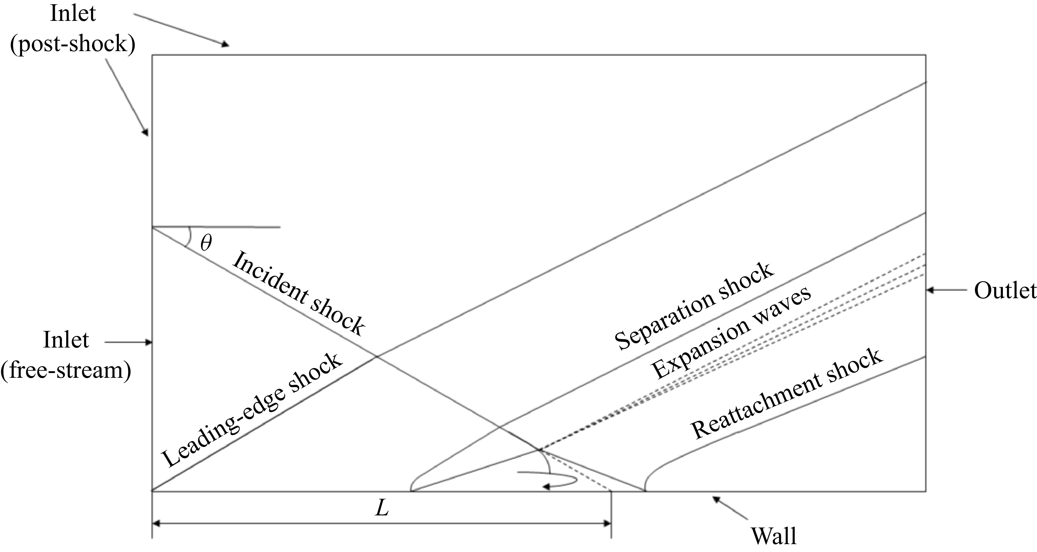
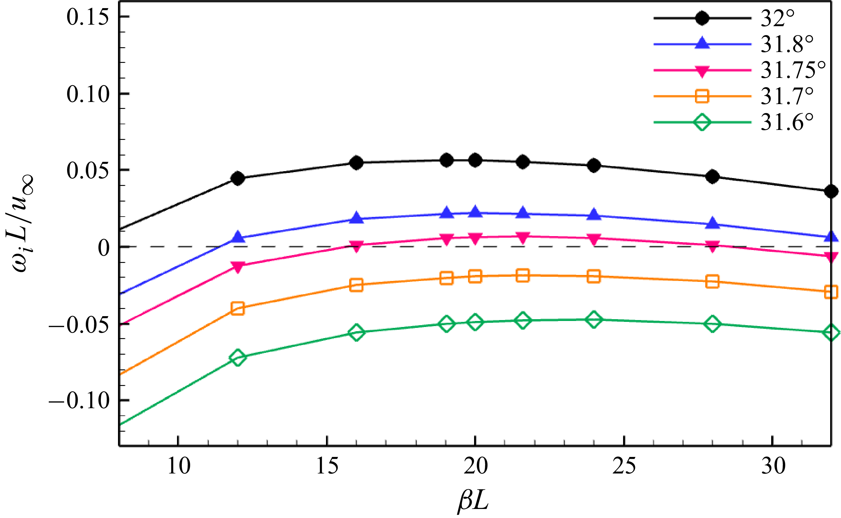
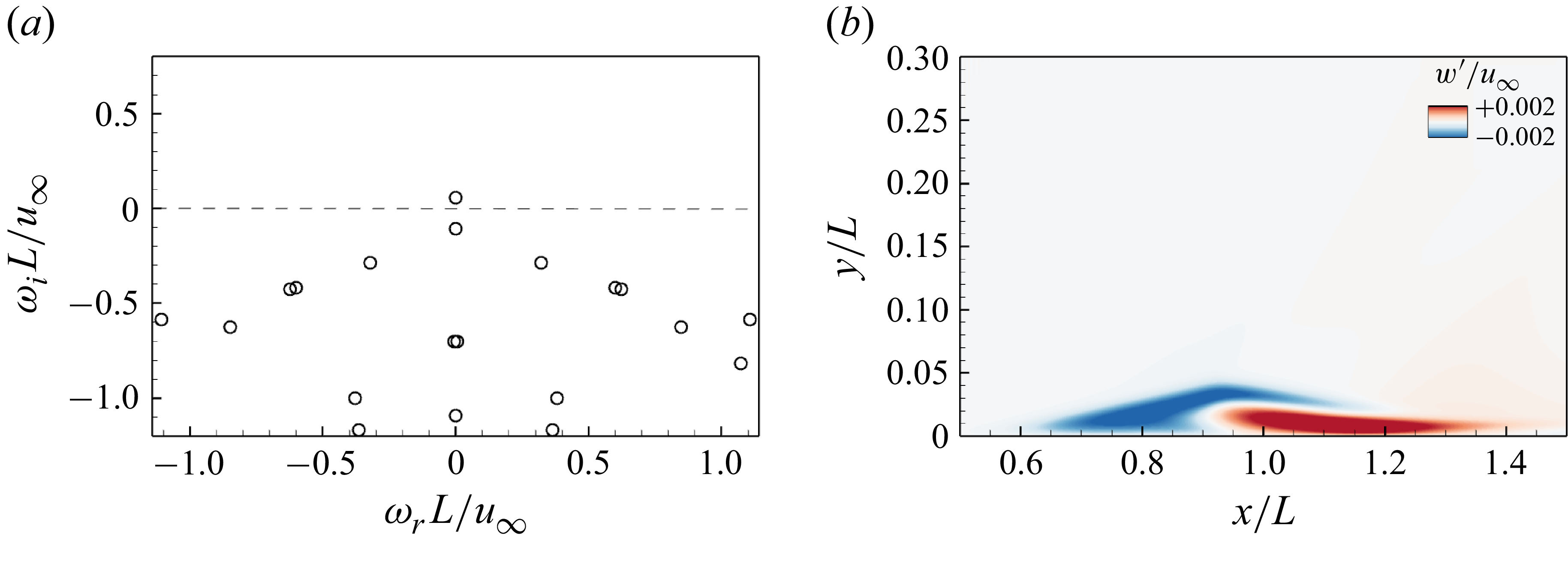
 βmL=19
 θ=32∘
 w′

 x/L=1
 θ=32∘
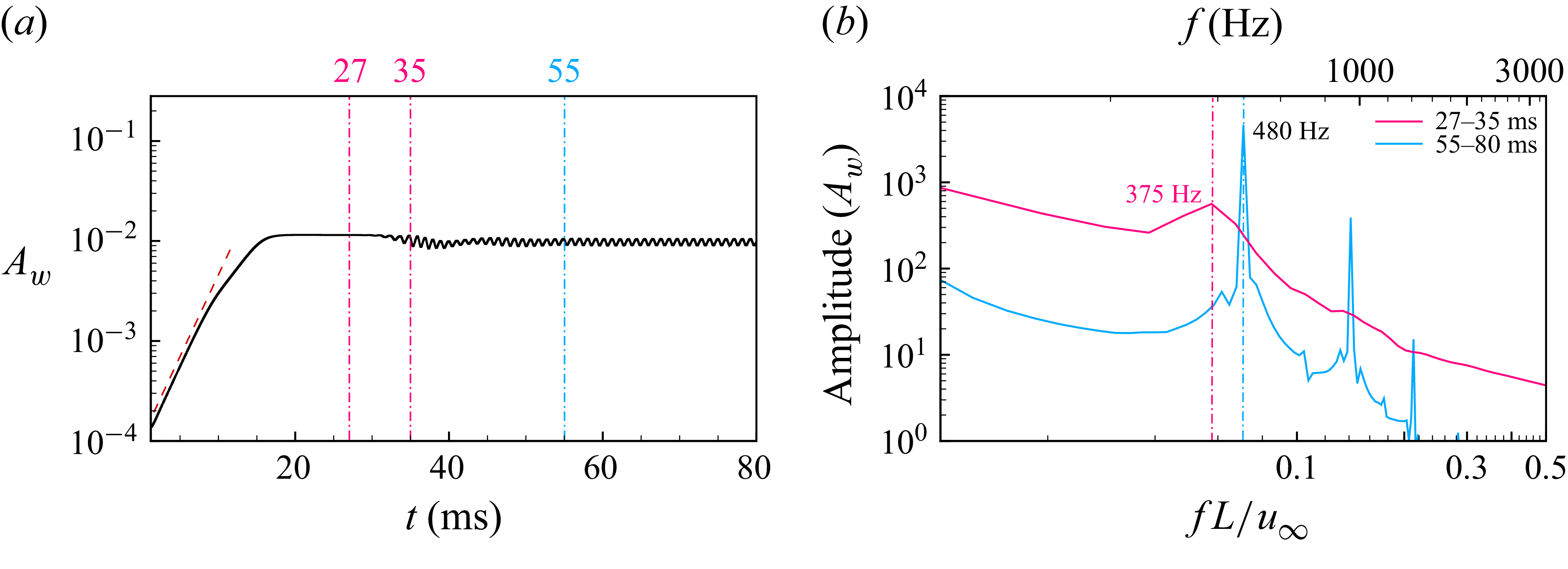
 Aw
 x/L=1
 λm
 θ=32∘
 Aw

 y/L=0.01
 λm
 θ=32∘

 x/L=1.125, y/L=0.009, z/L=0.083
 λm
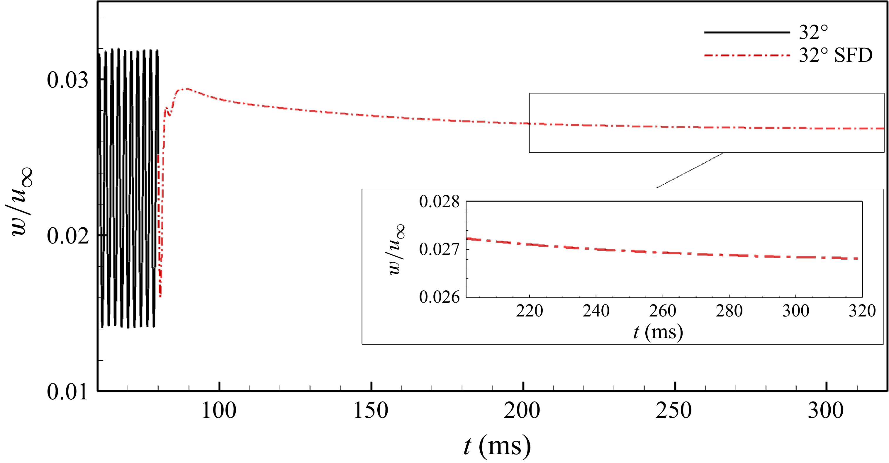
 λm
 θ=32∘
 x/L=1.125, y/L=0.009, z/L=0.083
 t=80ms

 t=320ms
 y/L=0.01
 λm
 θ=32∘
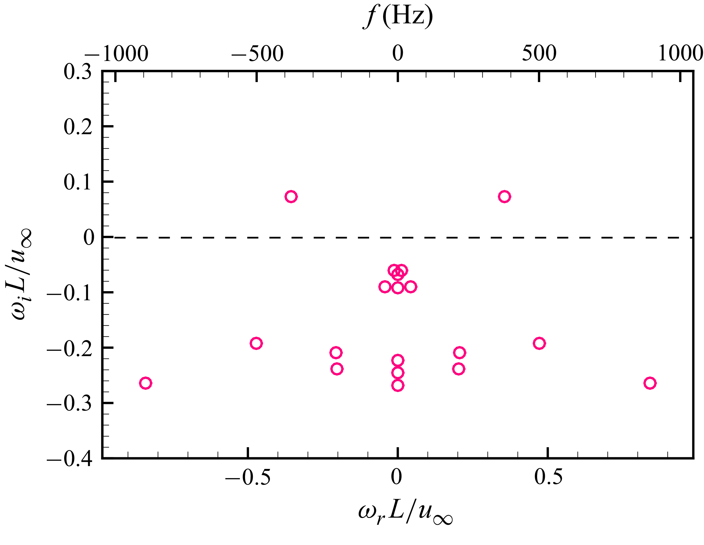
 λm
 θ=32∘

 λm
 θ=32∘

 x/L=1
 λm
 θ=32∘
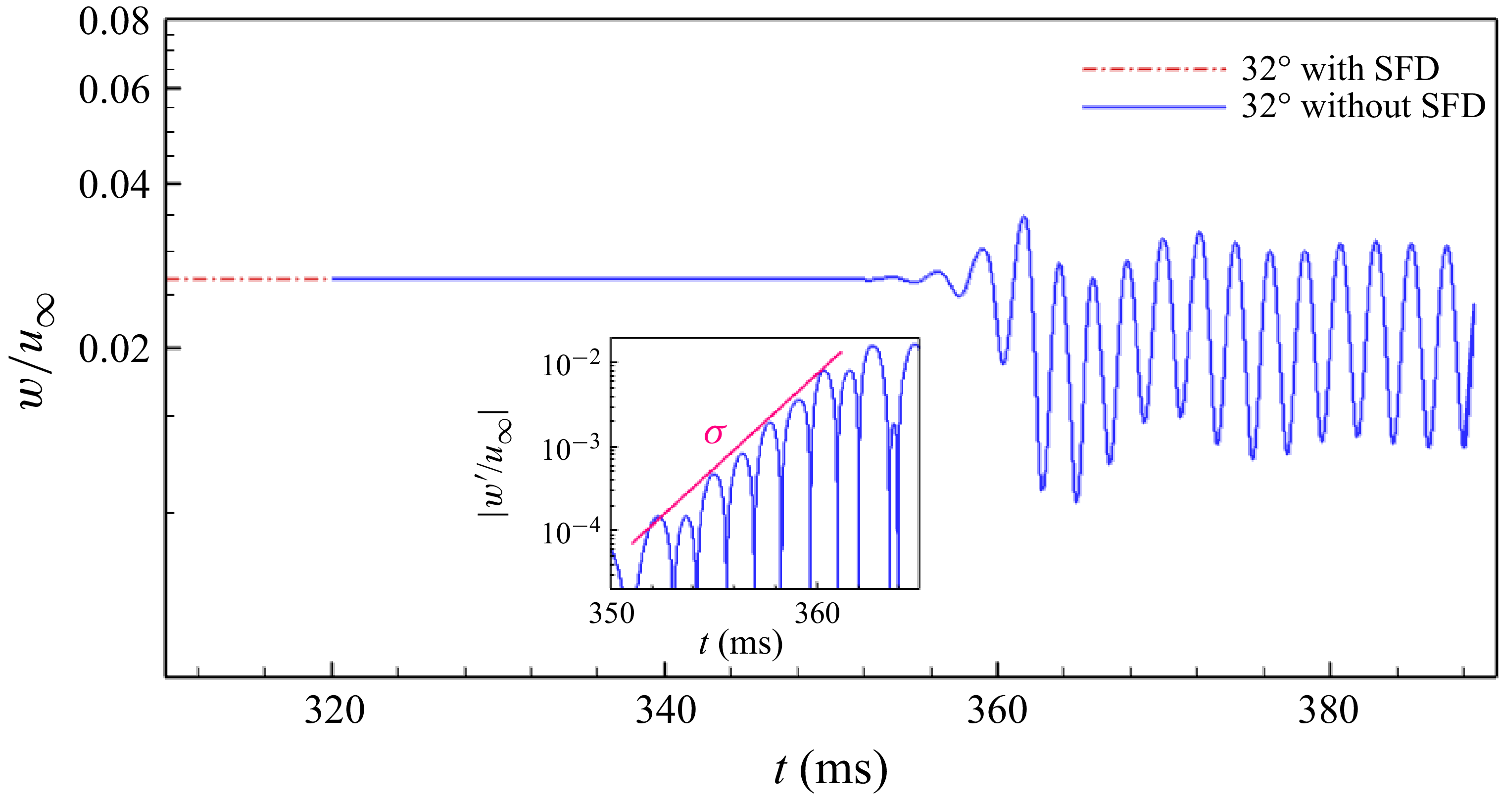
 λm
 θ=32∘
 x/L=1.125, y/L=0.009, z/L=0.083
 t=320ms

 t=358ms
 λm
 θ=32∘
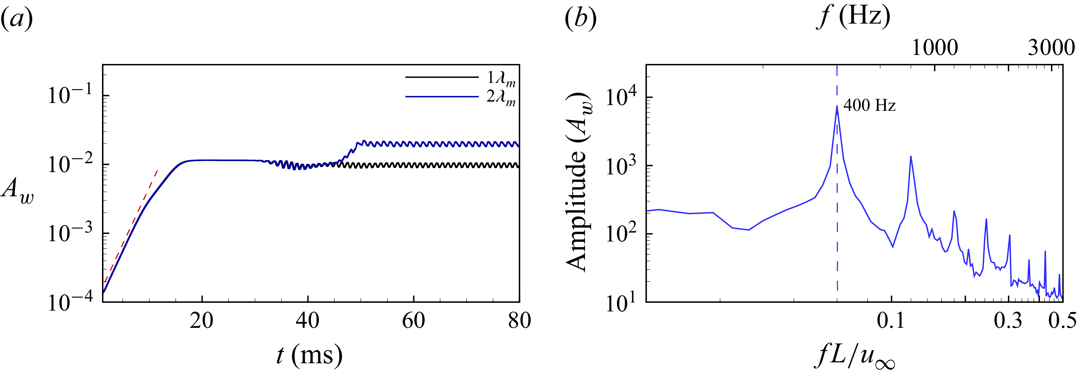
 Aw
 x/L=1
 2λm
 θ=32∘
 Aw
 60−80ms

 y/L=0.01
 2λm
 θ=32∘

 x/L=1.125, y/L=0.009, z/L=0.083
 2λm
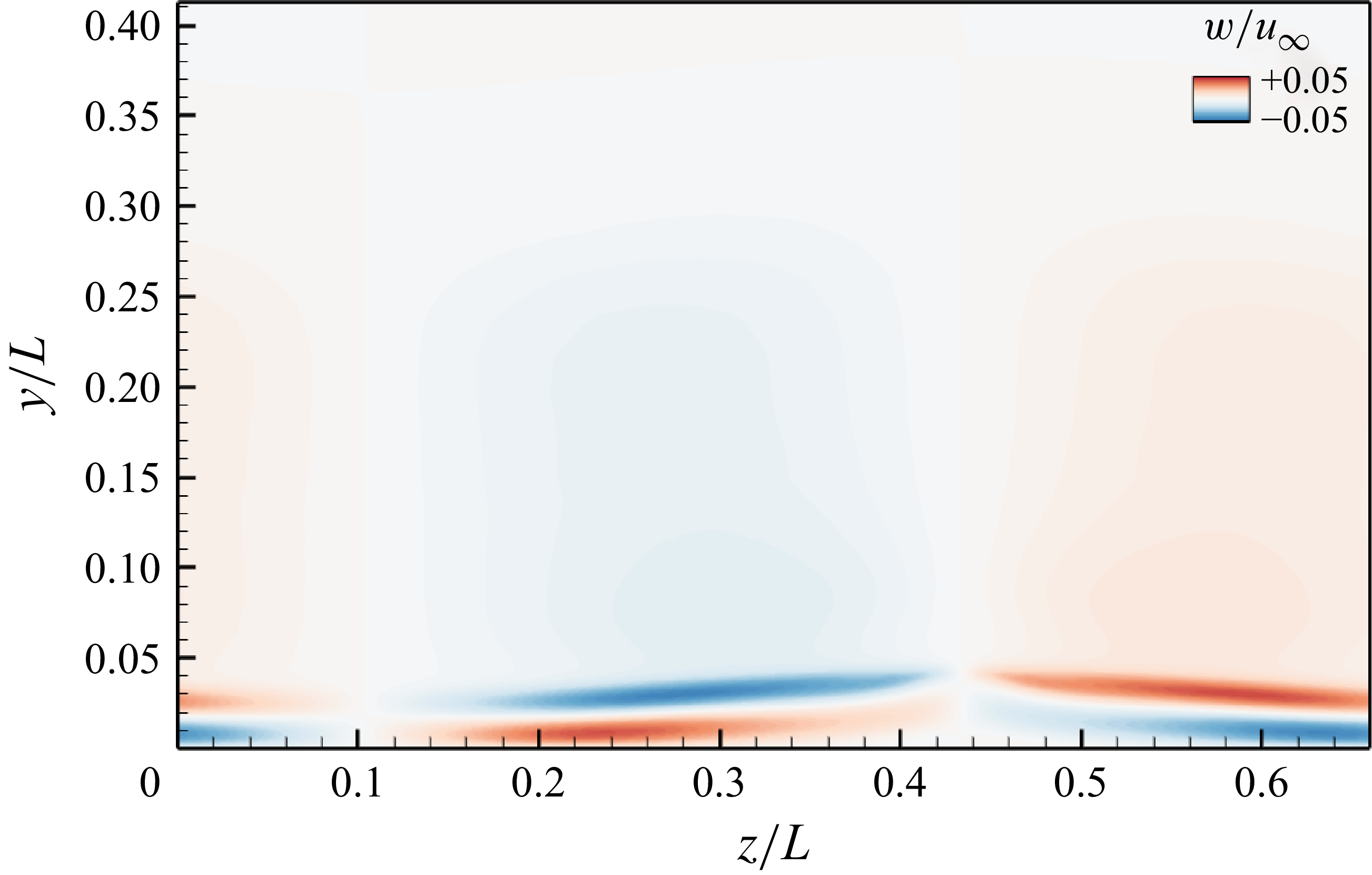
 x/L=1
 θ=31.2∘
 2λm
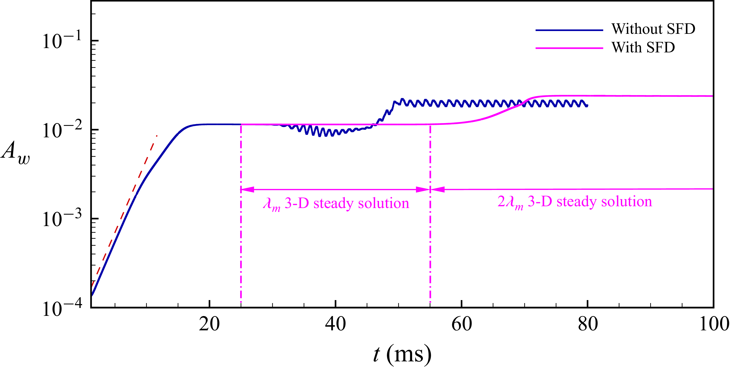
 Aw
 x/L=1
 θ=32∘
 2λm

 2λm
 θ=32∘
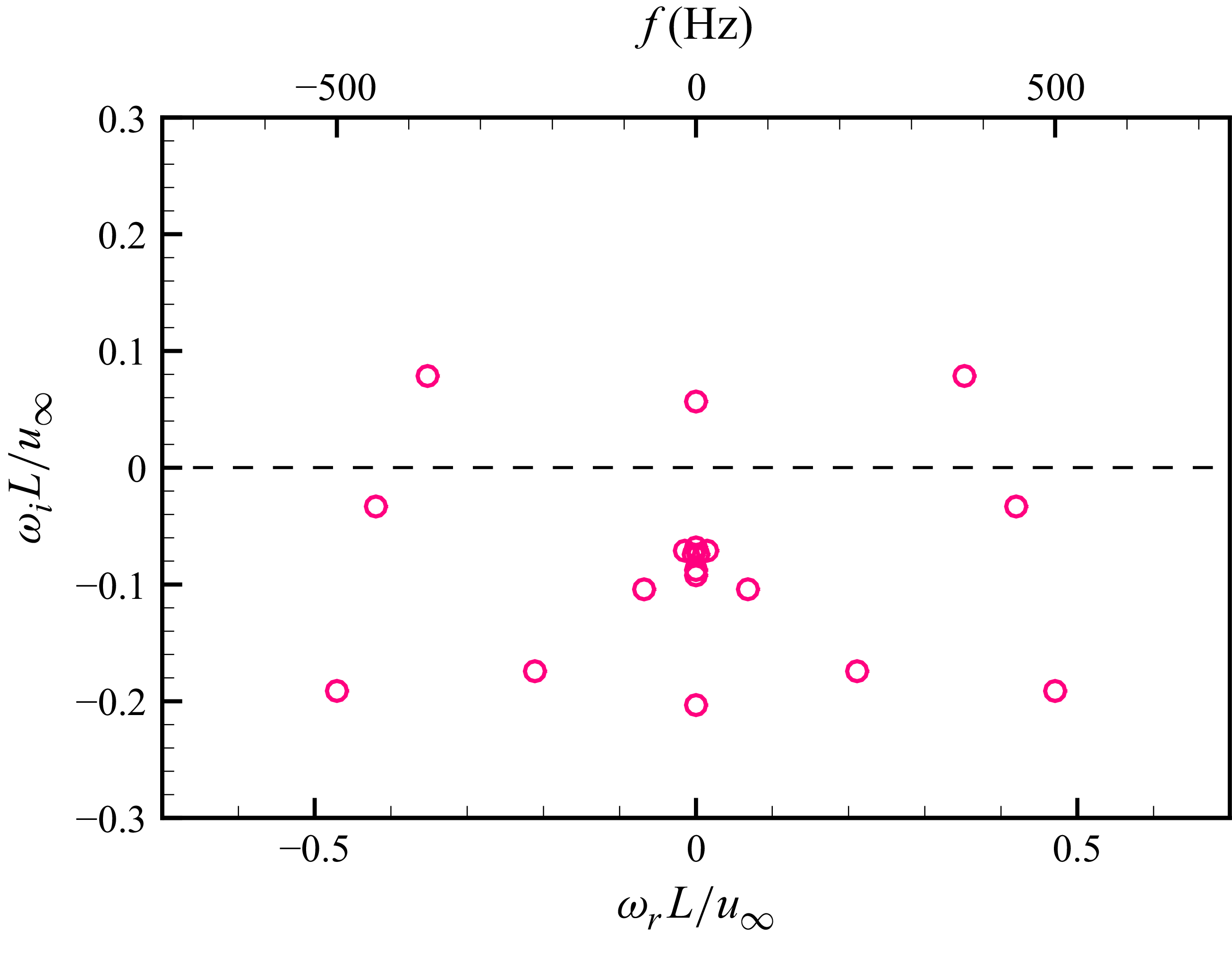
 2λm
 θ=32∘

 2λm
 θ=32∘
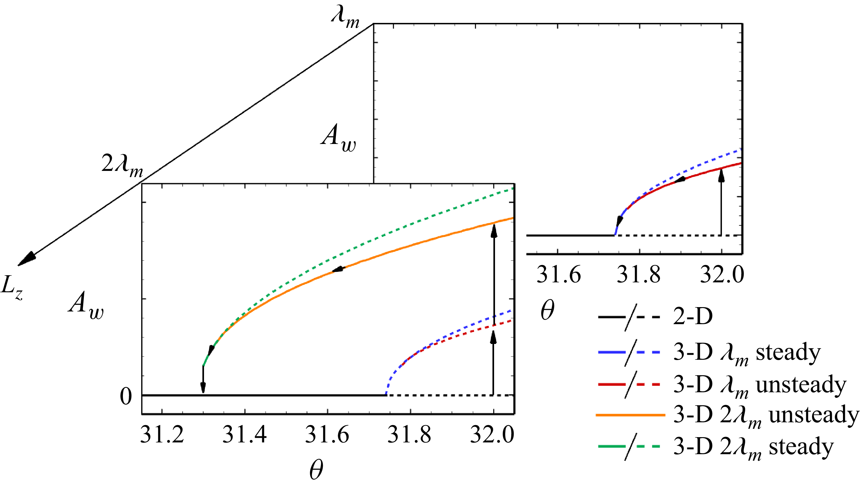
 θ
 Aw
 Lz
 Aw
 θ
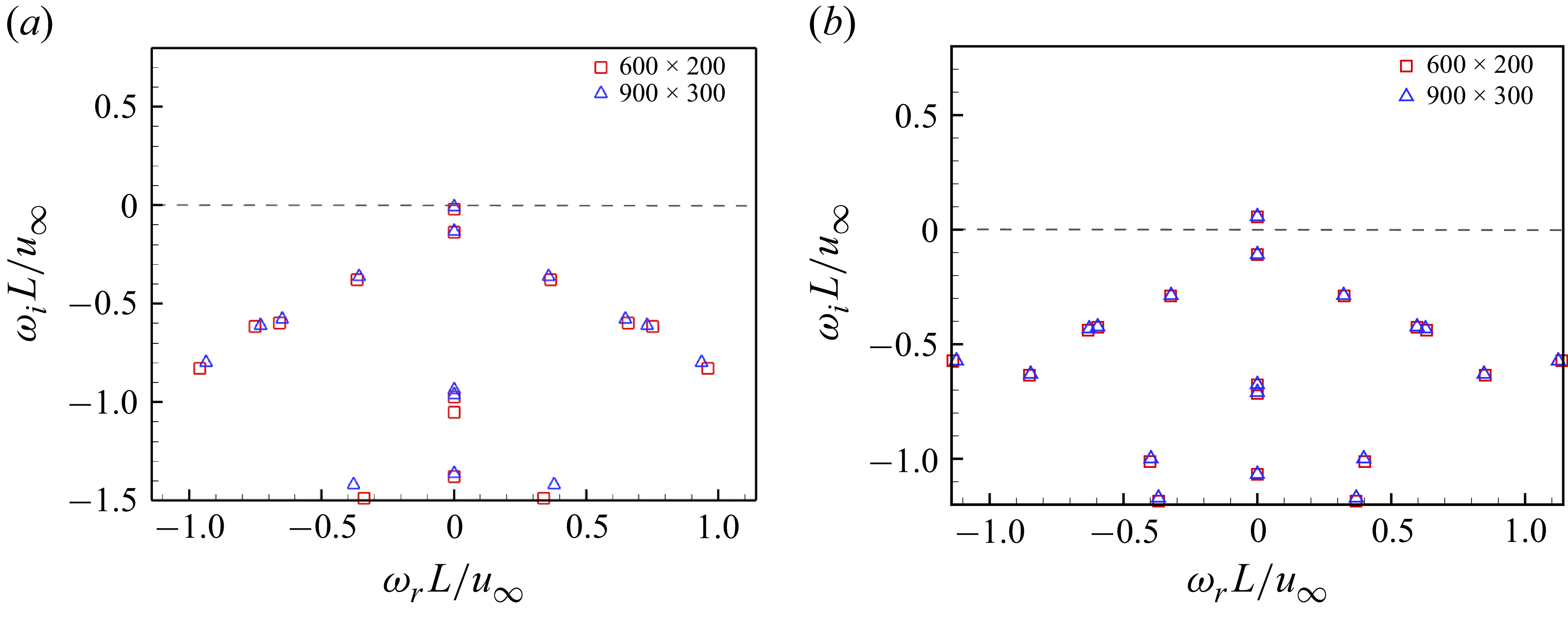
 θ=31.7∘
 θ=32∘
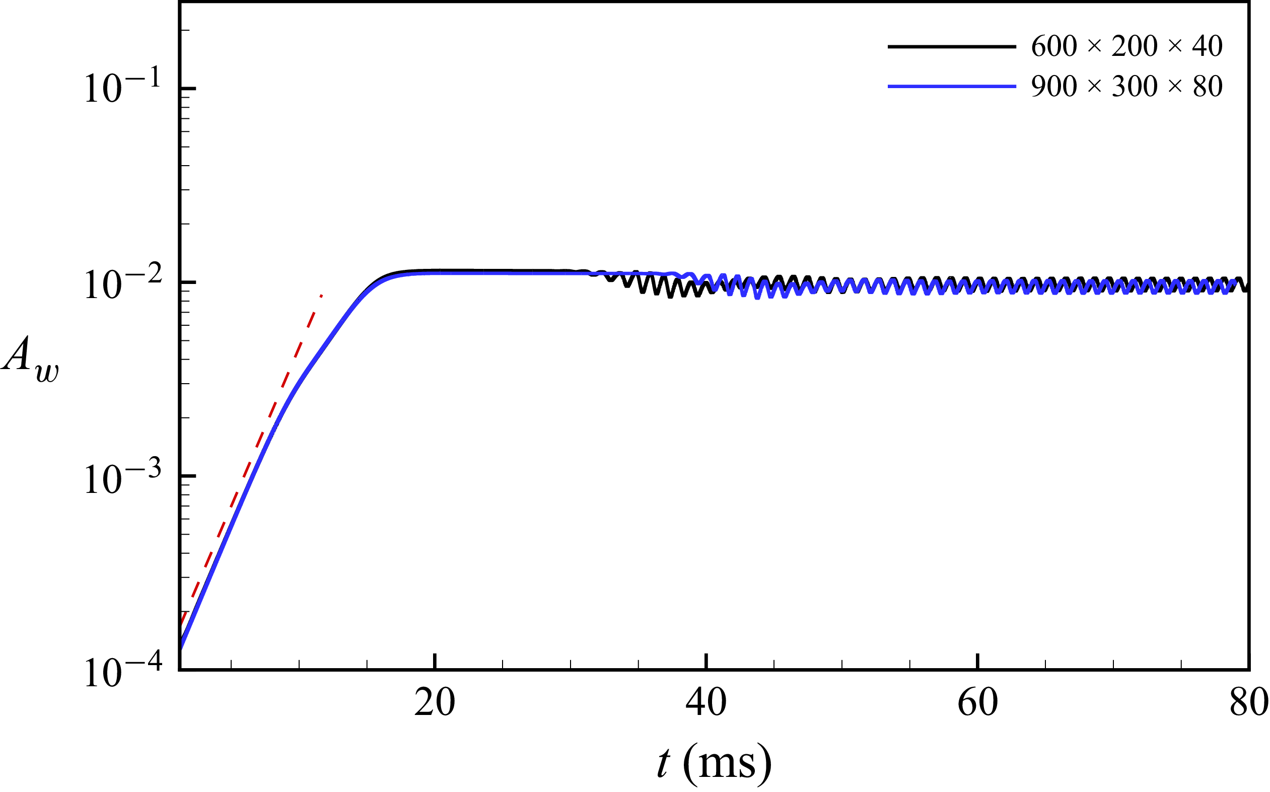
 Aw
 x/L=1
 λm
 θ=32∘
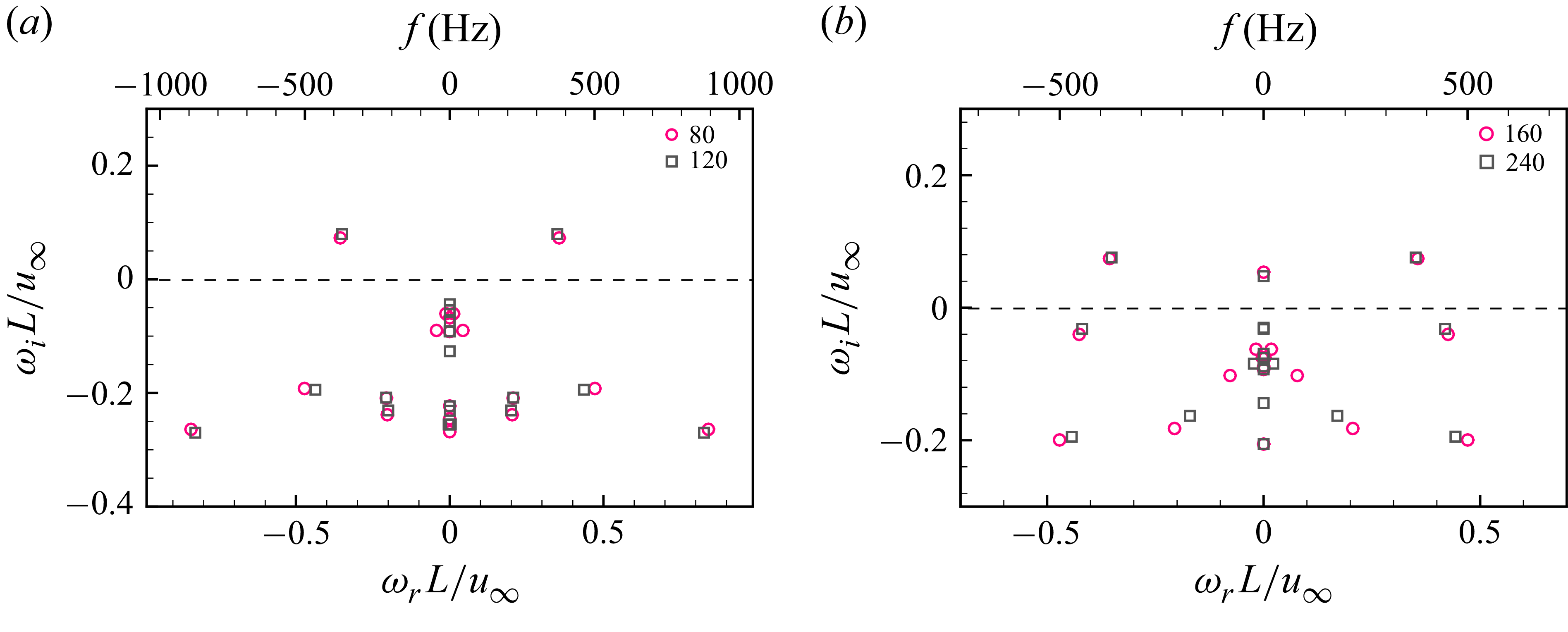
 θ=32∘
 λm
 2λm
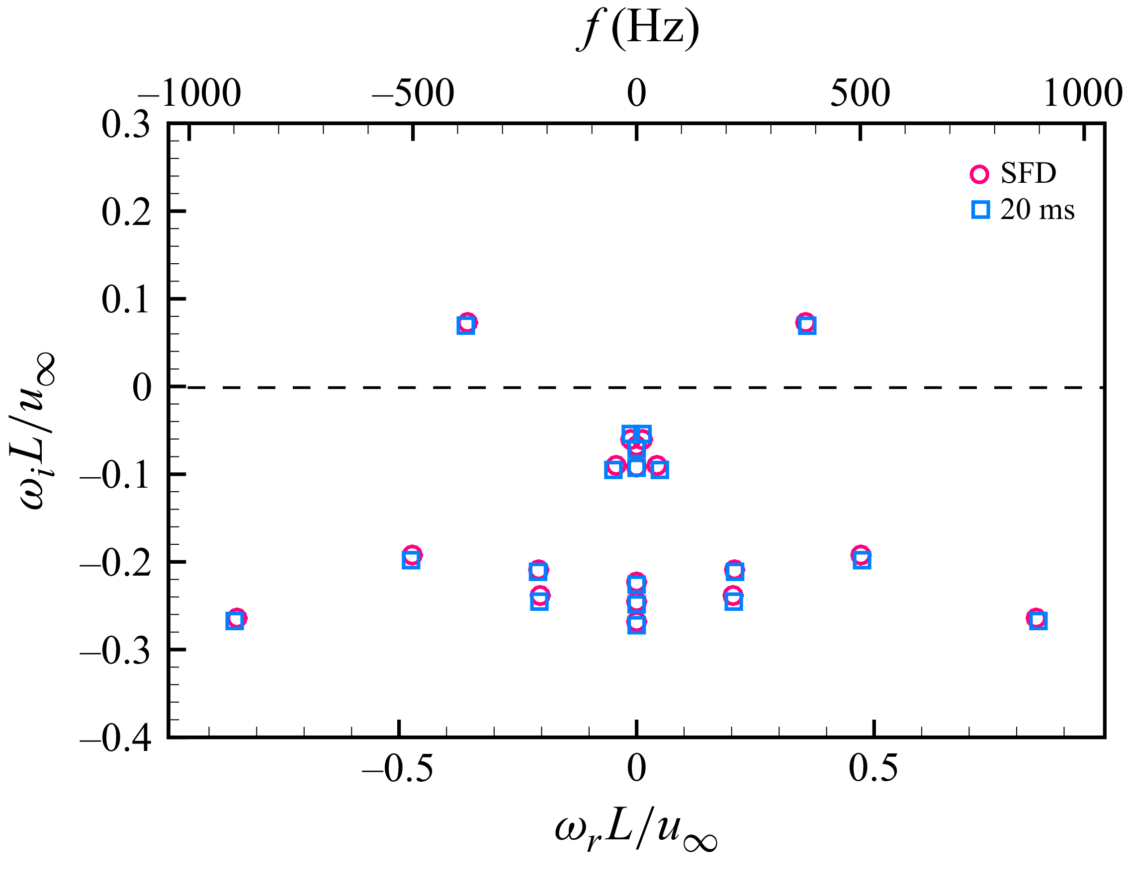
 λm
 t=20ms
 θ=32∘

 λm
 t=20ms
 θ=32∘
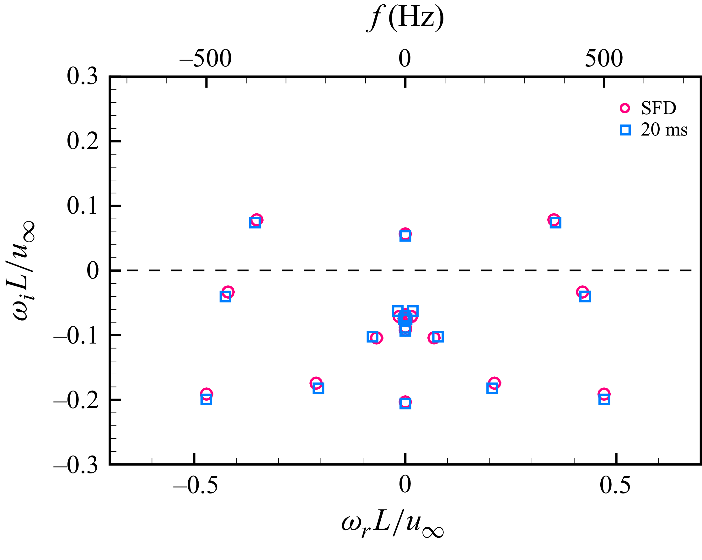
 2λm
 t=20ms
 θ=32∘

 2λm
 t=20ms
 θ=32∘
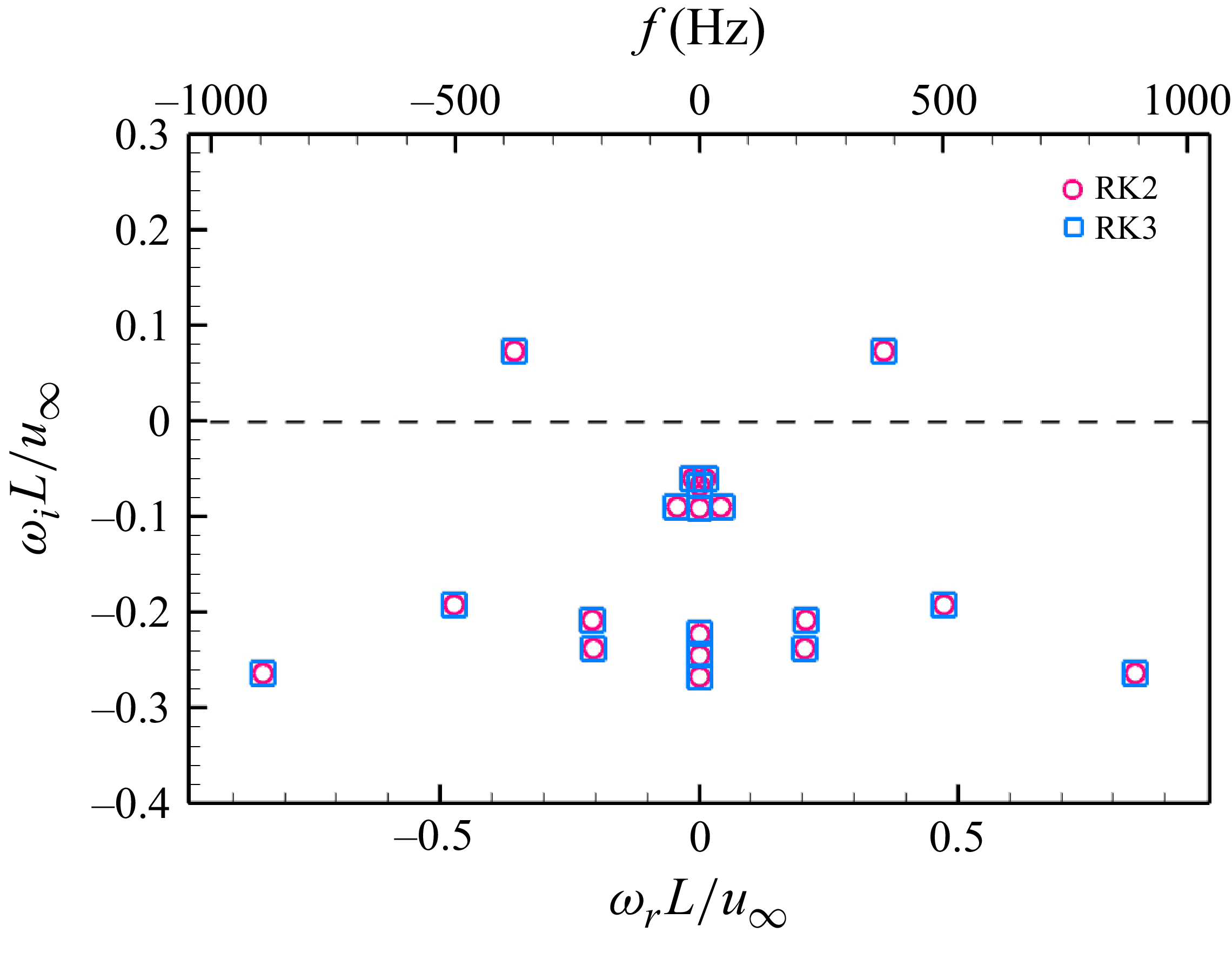
 λm
 θ=32∘
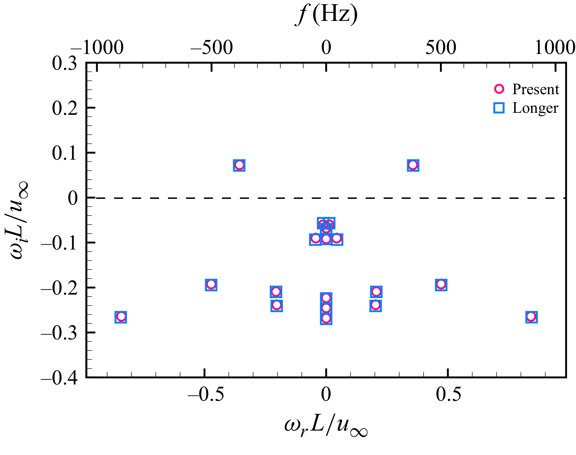
 λm
 θ=32∘
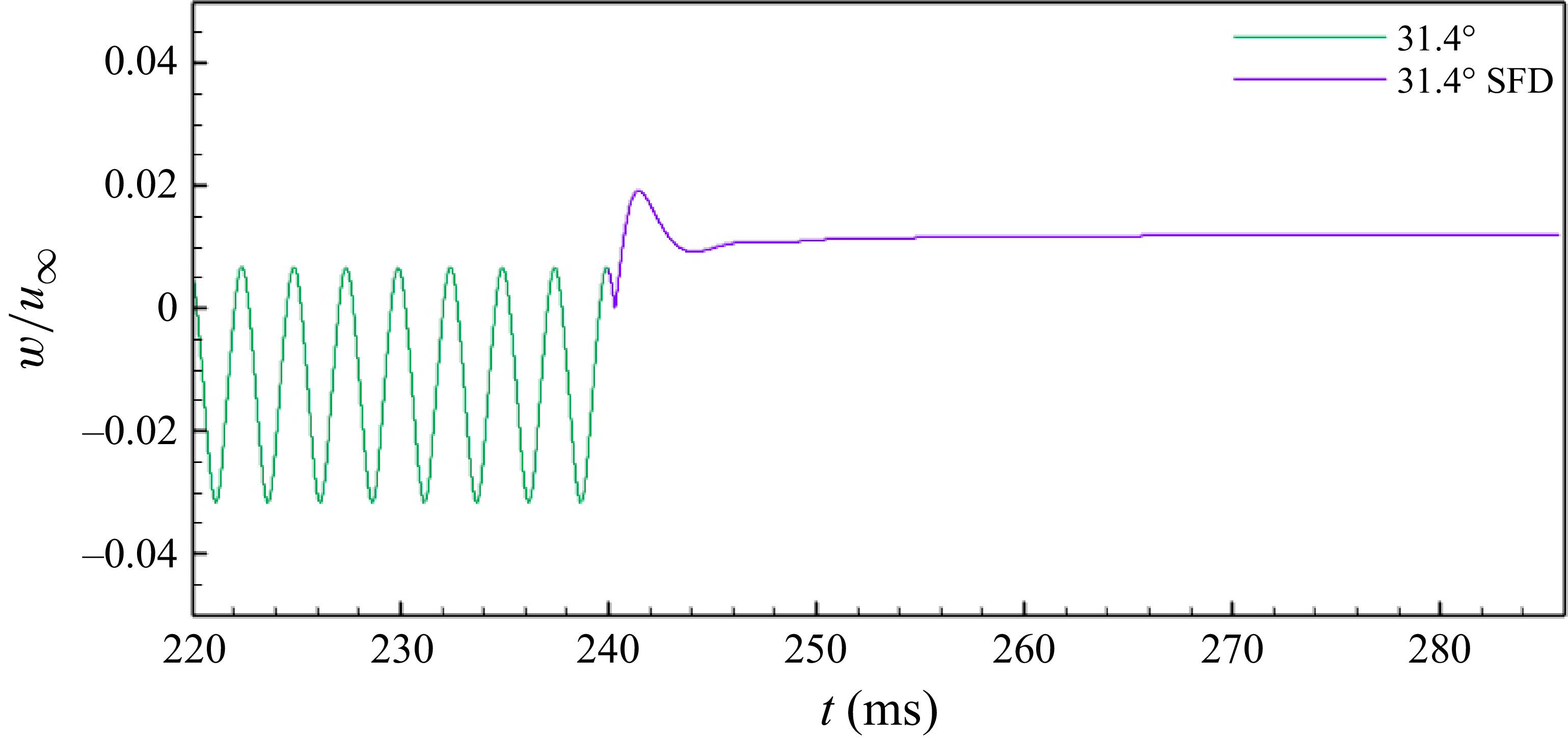
 θ=31.4∘
 2λm
 x/L=1.125, y/L=0.009, z/L=0.083
 t=240ms
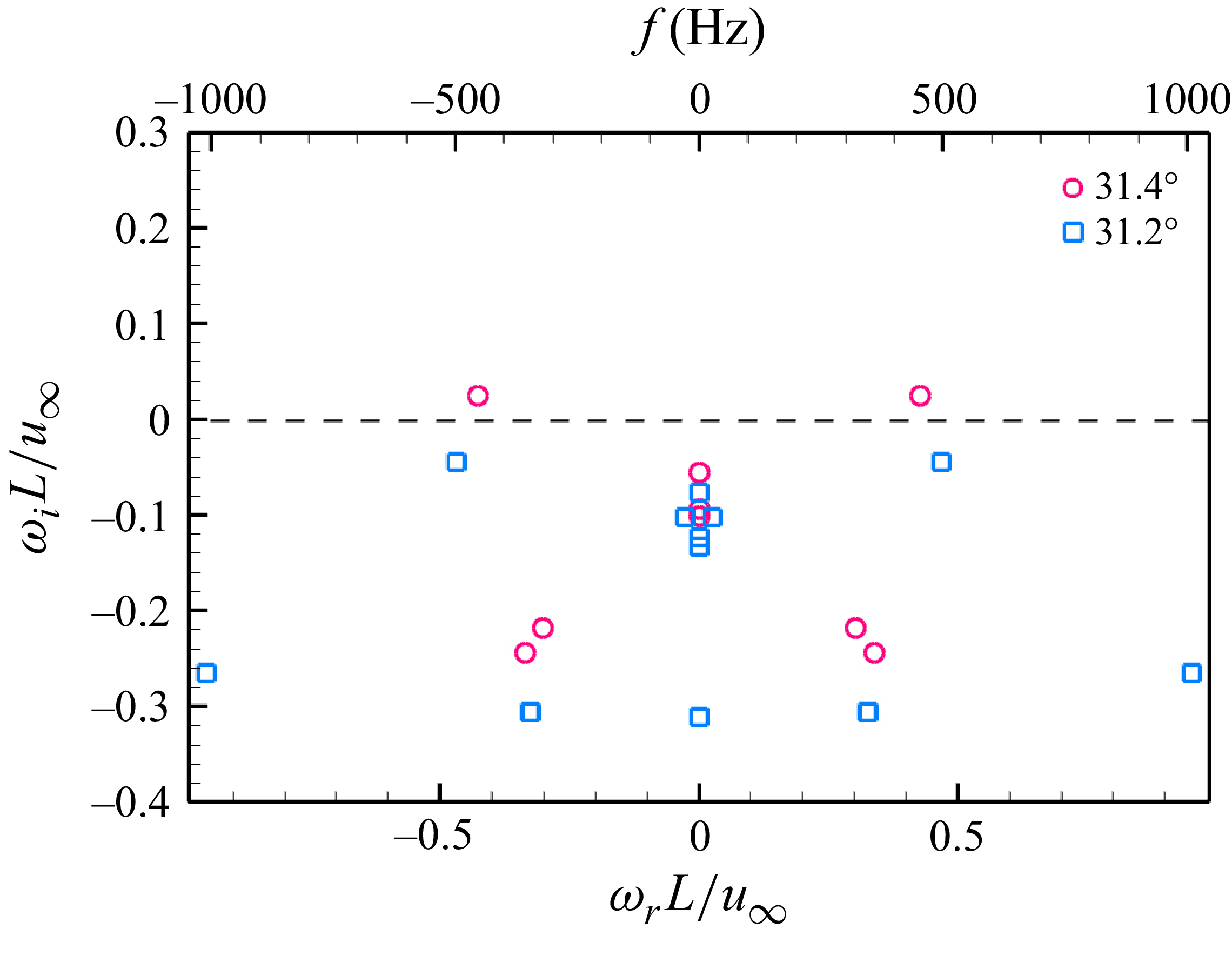
 2λm
 θ=31.4∘
 θ=31.2∘

 2λm
 θ=31.4∘


 Open access

