1 Introduction
Breakdown to turbulence in boundary layers exposed to moderate levels of free-stream turbulence is often preceded by the amplification of highly energetic streaks and their secondary instability. The recent study by Hack & Zaki (Reference Hack and Zaki2014a ) showed that linear instability analysis applied to cross-flow planes can capture the properties of the instabilities and identify the streaks that will likely induce transition to turbulence farther downstream. The present work compares the characteristics of those streaks to the remainder of the population and examines whether a data-based approach using artificial neural networks (ANN) can further improve the accuracy and the performance of the predictions to the levels required in real-time applications.
1.1 Streak instabilities in pre-transitional boundary layers
Boundary layers subjected to moderate levels of free-stream perturbations frequently bypass the natural transition mechanism via Tollmien–Schlichting waves and break down to turbulence earlier upstream. At the core of the bypass process is the growth of streamwise elongated perturbations known as Klebanoff streaks. The origin of the highly energetic streaks lies in the displacement of the mean momentum of the boundary layer due to small wall-normal velocity perturbations (Landahl Reference Landahl1975, Reference Landahl1980). Although the mean shear generally shields the boundary layer from external disturbances (Hunt & Carruthers Reference Hunt and Carruthers1990), this so-called shear sheltering is weakest for the low-frequency disturbances (Zaki & Saha Reference Zaki and Saha2009) which are most effective in generating streaks (Gustavsson Reference Gustavsson1991; Butler & Farrell Reference Butler and Farrell1992; Zaki & Durbin Reference Zaki and Durbin2005). The streaks promote the growth of high-frequency secondary instabilities which ultimately induce the nonlinear processes associated with breakdown to turbulence. The present focus is on the attributes of streaks that are linked to their secondary instability and, as a result, the onset of turbulence spots (for a review of the entire bypass transition process, see Zaki (Reference Zaki2013)).
In flow visualizations, streak instabilities are often observed as localized undulations of the host streaks (see e.g. Matsubara & Alfredsson Reference Matsubara and Alfredsson2001) that can be either varicose or sinuous. The controlled experiments by Asai, Minagawa & Nishioka (Reference Asai, Minagawa and Nishioka2002) excited both modes of streak instabilities in boundary layers and showed that the varicose mode induces hairpin vortices while the sinuous mode generates a train of quasi-streamwise vortices with vorticity of alternating sign. Elofsson, Kawakami & Alfredsson (Reference Elofsson, Kawakami and Alfredsson1999) generated streak-like structures in plane Poiseuille flow using wall blowing and suction and evaluated the phase speed and growth rates of the secondary instabilities. The experimental work by Mans, de Lange & van Steenhoven (Reference Mans, de Lange and van Steenhoven2007) examined five streaks in boundary layers exposed to static grid turbulence. Particle image velocimetry (PIV) studies by Mandal, Venkatakrishnan & Dey (Reference Mandal, Venkatakrishnan and Dey2010) identified inflectional instantaneous velocity profiles in streaky boundary layers which they credited with the amplification of varicose instabilities. Marquillie, Ehrenstein & Laval (Reference Marquillie, Ehrenstein and Laval2011) extracted individual low-speed streaks in channel flow subject to an adverse pressure gradient and performed instability analyses on the conditional average; they too predicted varicose-type instabilities. Meanwhile the nonlinear studies by Cossu et al. (Reference Cossu, Brandt, Bagheri and Henningson2011) identified threshold amplitudes for spanwise disturbances which lead to breakdown of streaks via a sinuous instability.
Vaughan & Zaki (Reference Vaughan and Zaki2011) classified the secondary instabilities of streaks into ‘outer’ and ‘inner’ modes based on the wall-normal locations of their critical layers. Phenomenological observations in direct numerical simulations (DNS) of bypass transition by Jacobs & Durbin (Reference Jacobs and Durbin2001) and Brandt, Schlatter & Henningson (Reference Brandt, Schlatter and Henningson2004) indicated that in zero-pressure-gradient (ZPG) boundary layers, breakdown to turbulence is predominantly initiated by outer instabilities situated on top of low-speed streaks at the edge of the boundary layer. Statistical data from DNS time series collected by Hack & Zaki (Reference Hack and Zaki2014a ) established that indeed more than 80 percent of all spot formations in ZPG boundary layers are preceded by an outer streak instability. That work also showed that an adverse pressure gradient significantly enhances the relevance of the inner instabilities.
Earlier investigations of streak instabilities by means of linear stability analysis considered idealized base states comprising streaks that were either steady (Andersson et al. Reference Andersson, Brandt, Bottaro and Henningson2001) or harmonic in time (Vaughan & Zaki Reference Vaughan and Zaki2011) and strictly periodic in the spanwise dimension. The predicted instabilities were therefore collective, i.e. of the entire row of streaks. Hack & Zaki (Reference Hack and Zaki2014a ) relaxed this condition by applying the instability analysis to cross-flow planes extracted from DNS of transitional boundary layers. Their base state hence comprised a spectrum of streaks with different amplitudes and proportions. The resulting instabilities were localized and could be attributed to individual streaks. This approach led to probability distributions for the amplitudes of the base streaks that induce the growth of the instabilities, in contrast to the discrete values for the critical streak amplitudes found in earlier studies. The implication is that, while the amplitude is an important factor, other properties of the base streaks, such as their shape and position in the cross-flow plane, are also relevant. These attributes have not been examined in the literature and are herein contrasted for innocuous streaks and the ones which initiate breakdown to turbulence.
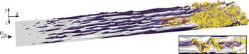
A visualization of a transitional boundary layer from DNS is presented in figure 1. Only particular streaks among the entire population promote the formation of turbulent spots via secondary instabilities. While linear analysis can identify those streaks and the secondary instability modes, the approach entails the solution of a computationally expensive eigenvalue problem and does not identify the streak characteristics which are complicit in promoting the secondary instability. A more nimble approach is sought herein to characterize the streaks in the pre-transitional boundary layer and to identify the subset of streaks that induce breakdown to turbulence.
Visualization of a streaky boundary layer undergoing bypass transition. Light isosurfaces are high-speed streaks (
 $u^{\prime }=0.085$
) and dark surfaces are low-speed streaks (
 $u^{\prime }=-0.085$
). Turbulence is visualized using isosurfaces of the
 ${\it\lambda}_{2}$
-criterion (
 ${\it\lambda}_{2}=-0.005$
).

1.2 Artificial neural networks
The concept of artificial neural networks can be traced back to the original perceptron devised by Rosenblatt (Reference Rosenblatt1958). It has since been successfully applied to a variety of tasks from different disciplines. A typical neural network of the kind used in the present work consists of a number of computing units, sometimes referred to as neurons in analogy to biology, which are arranged in layers. The output of each neuron is given by the evaluation of the associated basis function at the sum of all inputs. In so-called supervised learning, the network is initialized with random parameters and applied to a prototypical data set with known target values for the requested outputs. For example, by means of the popular backpropagation algorithm (see e.g. Rumelhart & McClelland Reference Rumelhart and McClelland1986), the weights that connect the neurons in different layers are adjusted so as to minimize the discrepancy between the predicted and target values, measured by a suitably chosen norm. ANN of sufficient complexity are universal approximators in the sense that, for an appropriate choice of parameters, such as network topology and number of neurons, they can represent any continuous function as long as the associated subspace is compact, i.e. closed and bounded (Hornik Reference Hornik1991).
In the field of fluid dynamics, several studies have sought to take advantage of the capabilities of artificial neural networks. Lee et al. (Reference Lee, Kim, Babcock and Goodman1997) employed ANN to construct an adaptive controller for reducing viscous drag in turbulent channel flow. The spanwise wall shear measured by an array of probes was used as input to the neural network, which was trained to produce a pattern of wall blowing and suction that reduced viscous drag by weakening near-wall turbulent streaks. Baldi & Hornik (Reference Baldi and Hornik1989) demonstrated that the training of an ANN with linear basis functions to perform an identity mapping on a data set effectively performs a linear principal component analysis (PCA) on these data. Building on this result, Milano & Koumoutsakos (Reference Milano and Koumoutsakos2002) constructed a nonlinear model of wall turbulence using a neural network with nonlinear basis functions. The nonlinear approach provided a more accurate model of the near-wall velocity fields at limited additional computational cost. More recently, Gautier et al. (Reference Gautier, Aider, Duriez, Noack, Segond and Abel2015) demonstrated a mechanism for the control of flow separation using genetic programming.
The present work aims to harness the capabilities of ANN in a novel approach to predict bypass transition in boundary layers. The objective is to efficiently and reliably identify the particular pre-transitional streaks that will eventually break down to turbulence via secondary instability. The velocity information in the DNS flow fields is compressed through the extraction of characteristic features of the boundary-layer streaks. These features differentiate properties of innocuous and unstable streaks. Although the latter represent a small fraction of the population, they are of principal importance in the laminar-to-turbulent transition process. These low-dimensional data are then passed on to an artificial neural network which provides a prediction of the likelihood of breakdown to turbulence. Section 2 provides analyses of streak data from DNS time series. In § 3, the prediction scheme, along with results for boundary layers subject to streamwise pressure gradients, are presented. Concluding remarks are presented in § 4.
2 Analysis of boundary-layer streaks
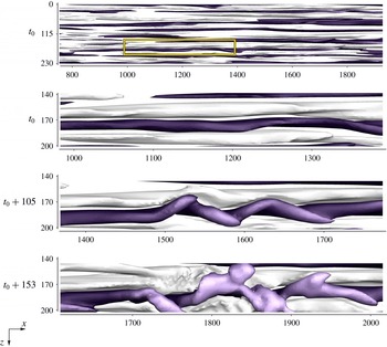
The starting point of the analysis is to contrast the streaks that cause breakdown to turbulence (referred to as B streaks) and the remainder of the population (referred to as NB streaks) by comparing attributes of both classes. Ahead of the presentation of the computational method and results, it is helpful to recall the physical mechanism of breakdown to turbulence in streaky boundary layers. While the low-frequency streaks are unable to directly initiate the short-scale nonlinear effects associated with the formation of turbulent spots, the shear surrounding the streaks promotes the growth of high-frequency exponential instabilities. A time series of a boundary-layer streak breaking down to turbulence via such instability is provided in figure 2. The topmost panel shows the entire spanwise extent of the computational domain in a ZPG boundary layer. Light and dark isosurfaces mark high-speed and low-speed streaks, respectively. From the second frame, the visualization focuses on a single low-speed streak located near the edge of the boundary layer. At later times, the instability increasingly distorts the base streak until the high-frequency oscillations induce nonlinear interactions and a turbulent spot emerges. The sinuous nature of the streak deformation is typical for the class of outer instabilities which account for the majority of streak breakdowns in zero- and favourable-pressure-gradient boundary layers. Inner modes, which originate from the local shear at the intersection of high and low-speed streaks inside the boundary layer, only become dominant in the presence of strongly adverse pressure gradients. The present study hence focuses on the outer type of streak instability.
Breakdown of a boundary-layer streak via sinuous outer instability. Plan view with isosurfaces of high-speed (
 $u^{\prime }=0.085$
, light) and low-speed streaks (
 $u^{\prime }=-0.085$
, dark). The shade of the low-speed streaks is indicative of the distance to the wall.

In the following, the computational approaches used in the flow simulations and in the analysis of the boundary-layer streaks are described. The remainder of the section is dedicated to a quantitative characterization of the B and NB populations of streaks.
2.1 Computational aspects and feature extraction
The flow fields in the present study are computed from DNS of transitional boundary layers. Descriptions of the simulation set-up and mean-flow statistics are provided by Nolan & Zaki (Reference Nolan and Zaki2013). The computational algorithm is based on a finite-volume formulation of the incompressible Navier–Stokes equations (Rosenfeld, Kwak & Vinokur Reference Rosenfeld, Kwak and Vinokur1991). Mass conservation is enforced using the fractional step method by Kim & Moin (Reference Kim and Moin1985). Velocities are normalized by the free-steam convective speed at the inlet of the computational domain,
 $U_{\infty ,0}$
, and lengths are normalized by the momentum thickness at that location,
 ${\it\theta}_{0}$
. The Reynolds number based on the inlet momentum thickness is
 $Re_{0}=108$
. The simulation domain starts at position
 $\tilde{x}_{0}$
downstream of the leading edge and the shifted streamwise coordinate is
 $x=\tilde{x}-\tilde{x}_{0}$
. The length, width and height of the computational domain are 4300, 285 and 215 inlet momentum thicknesses, respectively, and the number of grid points in these dimensions are 2049, 193 and 193. Bypass transition is initiated by superimposing the Blasius profile at the inflow of the computational domain with an isotropic free-stream disturbance field. The turbulence intensity in the free stream at the inflow is
 $Tu_{\mathit{FS}}=3\,\%$
. During the runtime of the simulations, a total of 4000 three-dimensional snapshots of the instantaneous flow fields are stored. The velocity fluctuations are computed from the instantaneous velocity field by subtracting a time and spanwise averaged mean,
 $$\begin{eqnarray}\boldsymbol{u}^{\prime }(x,y,z,t)\equiv \boldsymbol{u}(x,y,z,t)-\overline{\boldsymbol{u}}(x,z).\end{eqnarray}$$
In addition to a ZPG case, a favourable-pressure-gradient (FPG) boundary layer with Hartree parameter
 ${\it\beta}_{H}=0.11$
and a case with weakly adverse pressure gradient (APG),
 ${\it\beta}_{H}=-0.07$
, are considered. In the work by Nolan & Zaki (Reference Nolan and Zaki2013), a stronger adverse pressure gradient (
 ${\it\beta}_{H}=-0.14$
) was also simulated, where the inner instability was the dominant mechanism. For this reason, we have not considered that case in the present work where the focus in on the prediction of outer streak instabilities which are the prevalent mechanism over a wide range of flow configurations.
The skin-friction coefficient,
 $$\begin{eqnarray}C_{f}=\frac{{\it\mu}\left.{\displaystyle \frac{\partial U}{\partial y}}\right|_{y=0}}{{\textstyle \frac{1}{2}}{\it\rho}U_{\infty }^{2}(x)},\end{eqnarray}$$
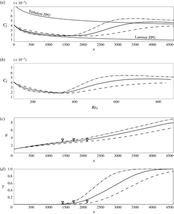
is plotted in figure 3(a) versus the streamwise coordinate,
 $x$
, for all cases. Earlier studies reported that in the presence of moderate levels of free-stream disturbances, the transition locations recorded for different pressure gradients nearly collapsed when plotted as a function of the momentum thickness (see e.g. Dunham Reference Dunham and Surugue1972). The present results show a similar tendency. In figure 3(b), the skin-friction coefficient is repeated as a function of the momentum thickness Reynolds number,
 $Re_{{\it\theta}}\equiv U_{\infty }(x){\it\theta}/{\it\nu}$
. In this scaling, the streamwise positions of transition onset for all three pressure gradients are in close proximity. The momentum thicknesses from the present simulations are reported in figure 3(c) as a function of the streamwise Reynolds number. The skin-friction minimum, which is commonly associated with the onset of transition, is also marked on the figure and is located at
 ${\it\theta}\approx 3$
in all three flow configurations. Finally, figure 3(d) shows the local intermittency, defined as the fraction of time during which the flow at a specific location is turbulent.
(a) Skin-friction coefficient
 $C_{f}$
as a function of the streamwise coordinate
 $x$
. (b) Skin-friction coefficient
 $C_{f}$
as a function of the momentum thickness Reynolds number
 $Re_{{\it\theta}}$
. (c) Momentum thickness
 ${\it\theta}$
as a function of the streamwise coordinate
 $x$
. (d) Intermittency
 ${\it\gamma}$
as a function of the streamwise coordinate
 $x$
. ZPG (solid), FPG (dashed) and APG (dash-dotted) cases.

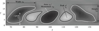
Streak features in a cross-plane. Background contours give the streamwise velocity fluctuation,
 $u^{\prime }$
. Contour lines at
 $u^{\prime }=0.05$
(black) and
 $u^{\prime }=-0.05$
(white) indicate the region of interest of each streak.

The analysis of the properties of the streaks is performed in cross-planes of the DNS flow fields such as the example in figure 4. The background contours mark the streamwise velocity fluctuation,
 $u^{\prime }$
. Black and white line contours identify
 $u^{\prime }=0.05$
, and
 $u^{\prime }=-0.05$
, and delimit the respective region of interest for each streak,
 ${\it\Omega}_{s}$
. The following features are extracted from the streaks.
-
(i) Peak streamwise intensity
 $s_{u}$
. The peak amplitude is defined as the maximum of the absolute of the streamwise velocity fluctuation,
$s_{u}\equiv \max _{{\it\Omega}_{s}}|u^{\prime }|$
.
-
(ii) Peak wall-normal intensity
$s_{v}$
. The maximum of the absolute of the wall-normal fluctuation is defined as
$s_{v}\equiv \max _{{\it\Omega}_{s}}|v^{\prime }|$
. Although the streaks are predominantly streamwise velocity perturbations, they are generated by the lift-up mechanism as a response to
$v^{\prime }$
forcing. In addition, wall-normal disturbances are amplified during the secondary instability of boundary-layer streaks prior to breakdown to turbulence. -
(iii) Area
$s_{A}$
. The cross-sectional area of the streak is computed as the integral of the region delimited by
${\it\Omega}_{s}$
, viz.
$s_{A}\equiv \int _{{\it\Omega}_{s}}\,\text{d}y\,\text{d}z$
. -
(iv) Momentum
$s_{M}$
. The streamwise momentum is related to the kinetic energy of the streak. It is computed as the integral of the streamwise velocity fluctuation over the region of interest,
$s_{M}=\int _{{\it\Omega}_{s}}u^{\prime }\,\text{d}y\,\text{d}z$
. -
(v) Spanwise shear
$s_{z}$
. The spanwise shear has been shown to correlate with the growth rate of outer streak instabilities (see Hack & Zaki Reference Hack and Zaki2014a
). It is approximated by dividing the peak streamwise fluctuation by half the streak width,
$s_{z}=2(s_{u}-0.05)/s_{W}$
, where the width is defined as the maximum extent of
${\it\Omega}_{s}$
in the spanwise dimension
$z$
,
$s_{W}=\max _{z}{\it\Omega}_{s}-\min _{z}{\it\Omega}_{s}$
. -
(vi) Wall-normal shear
$s_{y}$
. Although outer streak instabilities are primarily related to the spanwise shear, the wall-normal shear can be an important quantity to identify those streaks that develop instabilities. It is computed by dividing the peak streamwise fluctuation by half the streak height,
$s_{y}=2(s_{u}-0.05)/s_{H}$
, where the height is defined as the maximum extent of
${\it\Omega}_{s}$
in the wall-normal dimension
$y$
,
$s_{H}=\max _{y}{\it\Omega}_{s}-\min _{y}{\it\Omega}_{s}$
. -
(vii) Wall distance peak
$s_{d}$
. The distance between the wall and the location where the absolute value of
$u^{\prime }$
has its maximum,
$s_{y}=y_{s_{u}}$
. Since high-frequency free-stream perturbations are increasingly sheltered as they penetrate the boundary layer towards the wall, streaks that are lifted closer to the boundary-layer edge may have a higher chance of developing a secondary instability and inducing breakdown. -
(viii) Momentum thickness
$s_{{\it\theta}}$
. The local momentum thickness is directly related to the streamwise Reynolds number.













In order to contrast the properties of NB and B streaks, each streak in the DNS time series is assigned to one of the two classes by the following procedure: (i) recording of spot formation throughout the time series, (ii) identification of individual streaks, (iii) tracking of the streak evolution in time and (iv) association of spots with particular streaks.
The starting point is the capturing of the inception of turbulent spots in initially laminar flow. The spot detection algorithm starts from the approach introduced by Nolan & Zaki (Reference Nolan and Zaki2013), and is based on the local standard deviation of the sum of the
 $v^{\prime }$
and
 $w^{\prime }$
fluctuation fields. Applying the method by Otsu (Reference Otsu1979), the flow field is separated into laminar and turbulent regions such that the intra-class variance is minimized. The formation of a turbulent spot is recorded if an isolated region of turbulence is observed at a location that was occupied by laminar flow at the previous time step, and subsequently persists for at least 100 time units. This last condition makes the approach more robust by removing short-term ‘blips’ that may be the result of free-stream perturbations entering the boundary layer. The coordinates of the spot inception locations as well as the corresponding time in the flow evolution are stored in a database,
 $\boldsymbol{x}^{b_{m}}=\{x,y,z,t\}^{b_{m}}$
.
In a second step, the individual streaks in the time series of three-dimensional flow fields are identified. The streak detection procedure builds on the algorithm described by Nolan & Zaki (Reference Nolan and Zaki2013) and starts by computing the centroids of patches of positive and negative
 $u^{\prime }$
in cross-flow planes within the laminar flow regime. Streaks are identified by establishing the downstream connectivity of the extrema in the cross-flow planes. Objects whose length is less than a specified threshold, here 80 inlet momentum thicknesses, are discarded, and the coordinates of the centrelines of the remaining streaks are stored in a database,
 $\boldsymbol{x}_{t}^{s}=\{\boldsymbol{x},\boldsymbol{y},\boldsymbol{z};t\}^{s}$
.
In order to categorize streaks as B or NB, the entire history of each streak is gathered by tracking it in the time series. The outcome is a database which provides access to all instances of streaks via a unique identifier
 $\boldsymbol{x}^{s_{n}}=\{\boldsymbol{x}(t),\boldsymbol{y}(t),\boldsymbol{z}(t)\}^{s_{n}}$
. Finally, the streaks are linked to the spots. Since streaks are only identified in the laminar regime, they cannot coexist with a turbulent spot situated at the same coordinates. The algorithm therefore compares the spatial coordinates of the spots,
 $\boldsymbol{x}^{b_{m}}$
, with those of the streaks one snapshot prior to spot inception. Two databases are generated which contain the properties of the B and NB classes of streaks.
2.2 Comparison of
$\mathsf{B}$
and
$\mathsf{NB}$
streaks in ZPG boundary layers


The methodology described in § 2.1 allows a distinction between B and NB streaks. A comparison of the two classes can shed light on why particular streaks break down to turbulence. An overview of the difference between the two classes is provided by the conditionally averaged field at a given downstream position
 $x$
,
 $$\begin{eqnarray}\{\boldsymbol{u}^{\prime }\}_{\pm }(x,y,\tilde{z})\equiv \frac{1}{N_{\pm }}\mathop{\sum }_{n=1}^{N_{\pm }}\unicode[STIX]{x1D642}(z_{n\pm })\boldsymbol{u}^{\prime }(x,y,z_{n\pm }),\end{eqnarray}$$
where subscripts ‘
 $+$
’ and ‘
 $-$
’ denote high- and low-speed streaks, respectively. The linear operator
 $\unicode[STIX]{x1D642}(z_{n\pm })$
translates the velocity field for each streak in the span such that its local
 $u^{\prime }$
extremum is aligned at the spanwise location
 $\tilde{z}=0$
.
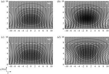
The conditional averages for low-speed streaks of classes B and NB at two different downstream locations are contrasted in figure 5. The number of samples is approximately 33 000 NB and 300 B. In all cases, the streamwise vortices which effect the lift-up process and lead to the amplification of streaks are evident. Comparison of the two classes indicates that streaks which belong to the B class (i.e. will induce breakdown to turbulence) have a relatively higher amplitude, particularly at
 $x=1754$
. They are also located farther away from the wall than their NB counterparts. Furthermore, the distance to the surrounding high-speed streaks appears to be smaller for B streaks than for NB structures, which suggests stronger spanwise shear. While the conditionally averaged
NB streaks resembles an ellipse, the B conditionally averaged structure develops into a trapezoidal shape. The widening near the edge of the boundary layer is in part a result of the streak meandering due to the amplification of secondary instabilities, see e.g. figure 2.
Conditionally sampled low-speed streaks not leading to breakdown (a,c) and leading to breakdown (b,d) at downstream positions
 $x=1321$
(
 ${\it\theta}=2.5$
, a,b) and
 $x=1754$
(
 ${\it\theta}=3$
, c,d). The background contour and lines indicate the streamwise velocity fluctuation,
 $-0.18<\{u^{\prime }\}_{-}<0.12$
. White lines mark
 $\{u^{\prime }\}_{-}=-0.05$
and indicate the conditionally sampled region of interest. Arrows give the spanwise and wall-normal fluctuations. The local boundary-layer thickness is marked by the dashed white line.

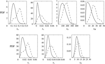
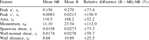
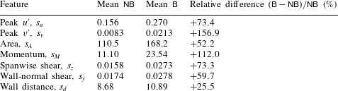
Probability density functions (PDFs) of the features of both classes of streaks are presented in figure 6. The respective mean values as well as the relative differences are reported in table 1. The results mirror the trend observed in the visualizations of the conditionally averaged flow field. All features have appreciably higher values in the case of B streaks. In particular, the peak streamwise and wall-normal fluctuations of the B streaks considerably exceed the values of the NB class.
Probability density functions of streak features for ZPG boundary layer.
 $\mathsf{NB}$
streaks (solid) and
 $\mathsf{B}$
streaks (dashed) at
 $x=1321$
(
 ${\it\theta}=2.5$
).

Mean values of features of
 $\mathsf{NB}$
and
 $\mathsf{B}$
streaks and relative difference in ZPG boundary layer at
 $x=1321$
(
 ${\it\theta}=2.5$
).
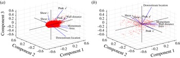
A principal component analysis (PCA) of the streak properties is presented in figure 7. The first three principal components are shown. In both the NB and B cases, the momentum and the area are closely correlated. On the other hand, there appears to be no direct link between
 $s_{u}$
and
 $s_{v}$
. Despite the vertical velocity contributing to the amplification of streaks, only the low-frequency component is relevant. In addition, the
 $v$
perturbations introduced by free-stream vortical disturbances decay appreciably while the streaks are formed and intensify (see e.g. Andersson, Berggren & Henningson Reference Andersson, Berggren and Henningson1999). The amplification of
 $v$
in the boundary layer occurs farther downstream when the secondary instabilities start to amplify. As a result,
 $s_{v}$
does not correlate well with
 $s_{u}$
. Although the principal components of the B and NB classes differ, in both cases the first three components describe virtually the same fraction (approximately 82 %) of the total variance of the eight features considered.
Principal component analysis of the features extracted from
 $\mathsf{NB}$
streaks (a) and
 $\mathsf{B}$
streaks (b).

2.3 Influence of streamwise pressure gradient
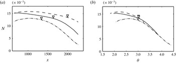
The skin-friction curves presented in figure 3(a) indicated that a favourable pressure gradient delays breakdown to turbulence while adverse pressure gradient promotes it. The question arises whether this behaviour is due to a change in the number of streaks in the boundary layer, or whether the size of the streak population remains unaffected. Figure 8(a) shows the frequency of occurrence of all boundary-layer streaks per unit spanwise width from both the NB and B classes. The frequency of occurrence is similar in all cases, but highest in the presence of the favourable pressure gradient and lowest for the adverse pressure gradient. The trend is consistent with the faster growth of the boundary-layer thickness in decelerating flow, and as a result the formation of wider streaks and lower number density in that case. This result also indicates that the early breakdown in the APG case is not due to an increased rate of streak formation. When plotted versus the momentum thickness, the three curves for the entire population converge downstream of transition onset. The similar decay rates across pressure gradients can be explained with reference to the spreading of turbulence spots in the transition zone. While the spread angle measured from the spot inception location is known to be wider in decelerated flows (see e.g. Gostelow, Melwani & Walker Reference Gostelow, Melwani and Walker1996), the volume growth rate of the turbulent patches is insensitive to the pressure gradient (see figure 30 by Nolan & Zaki Reference Nolan and Zaki2013). As a result, the streaks are depleted in the transition zone at a similar rate across the different pressure gradients.
Normalized frequency of occurrence of streaks versus (a) downstream coordinate
 $x$
and (b) momentum thickness
 ${\it\theta}$
. ZPG (solid), FPG (dashed) and APG (dash-dotted) cases. Symbols indicate the onset of transition to turbulence.

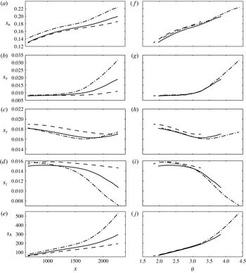
Other features of the populations of streaks also collapse when plotted as a function of the momentum thickness. Figure 9 shows the peak streamwise and wall-normal velocity fluctuation, the wall-normal and spanwise shear and the streak cross-sectional area versus
 ${\it\theta}$
for the ZPG, FPG and APG cases. The relative difference between the three cases is less than ten percent over the entire downstream range. These results demonstrate that the momentum thickness governs not only the location of transition onset in pressure-gradient boundary layers, but also the properties of the streaks.
Mean streak attributes as a function of the streamwise coordinate (a–e) and of the momentum thickness (f–j). ZPG (solid), FPG (dashed) and APG (dash-dotted) cases. (a,f) Peak streamwise amplitude, (b,g) peak wall-normal fluctuation, (c,h) wall-normal shear, (d,i) spanwise shear and (e,j) cross-section area.

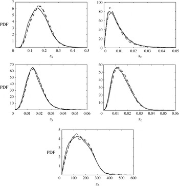
The significance of the momentum thickness as a scaling parameter for the streaks can be demonstrated further by considering PDFs recorded at identical
 ${\it\theta}$
. Normalized distributions of the peak amplitude, the cross-sectional area and the wall-normal and spanwise shear of the streaks at
 ${\it\theta}\approx 3$
are provided in figure 10. This location coincides with the onset of transition for all three pressure gradients. In each case, the curves representing the three different pressure gradients are in close agreement.
PDFs computed at
 ${\it\theta}=3$
. ZPG (solid), FPG (dashed) and APG (dash-dotted) cases. Peak streamwise amplitude, peak wall-normal fluctuation, wall-normal shear and spanwise shear and cross-section area.

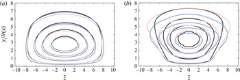
Corbett & Bottaro (Reference Corbett and Bottaro2000) investigated optimal growth in pressure-gradient boundary layers and found that the momentum thickness led to a ‘universal’ behaviour of the perturbation kinetic energy of the streaks. Here we compare the conditionally sampled
 $u$
-perturbation fields of NB and B streaks from the DNS of bypass transition. The results for streaks from the ZPG, FPG and APG cases at
 ${\it\theta}=3$
are presented in figure 11. For each class of streaks, the isocontours of the streamwise velocity fluctuation in the cross-flow plane largely coincide across pressure gradients. In particular, the deformation of the contours in case of the B streaks is present in all three flow conditions.
Isocontours of the streamwise fluctuation component,
 $\{u^{\prime }\}_{-}$
, of conditionally sampled low-speed streaks at
 ${\it\theta}=3$
. (a)
 $\mathsf{NB}$
streaks. (b)
 $\mathsf{B}$
streaks. ZPG (black), FPG (blue/dark grey) and APG (red/light grey) cases.

3 Feature-based classification of streaks
The analysis presented in § 2 showed that the properties of NB streaks can differ appreciably from those of B streaks. In the following we examine whether this information can be harnessed to predict breakdown to turbulence by using the features extracted from the streaks as inputs to an artificial neural network. The section starts with a brief description of the methodology followed by results for a ZPG boundary layer. Finally, the generalization abilities of the network are tested by examining the accuracy of the predictions in favourable and weak adverse pressure gradients.
3.1 Artificial neural network
ANN are universal approximators which can represent any continuous, smooth function. One of the most common applications of ANN is pattern recognition and classification where their capability to generalize, i.e. to correctly classify data contaminated by noise, is particularly useful. In the present case, the objective is to use combinations of the streak features extracted from the DNS time series in order to forecast whether a specific sample will induce breakdown to turbulence farther downstream.
Topology of the artificial neural network used in the present study.

The general topology of the neural network used in this study is presented in figure 12. The circles represent the computational units, or neurons, of the network, which are arranged in three layers. Each neuron in a specific layer is connected to all the neurons in the adjacent layers but not to neurons in its own layer. The connections between the neurons are associated with variable weights which determine the behaviour of the ANN. A sigmoid activation function is used so that the output (or activation) of each neuron is given by
 $$\begin{eqnarray}q_{k}^{n}=\frac{1}{1+\exp (-p_{k}^{n})}.\end{eqnarray}$$
Here,
 $n$
indicates the layer of the neuron and
 $k$
is the number of the computing unit within that layer. With the exception of the input layer (
 $n=1$
), the input into a neuron is the weighted sum of the activations of the neurons in the previous layer,
 $$\begin{eqnarray}p_{k}^{n}=\mathop{\sum }_{j}w_{k,j}^{n}q_{j}^{n-1},\end{eqnarray}$$
where the index
 $j$
spans all weights that connect the computing unit with all units on the previous layer
 $n-1$
. In terms of a matrix-vector product, equation (3.2) can be written as,
 $$\begin{eqnarray}\boldsymbol{p}^{n}=\unicode[STIX]{x1D652}^{n}\boldsymbol{q}^{n-1}.\end{eqnarray}$$
Let
 $\mathscr{N}^{n}$
denote the number of neurons on the
 $n$
th layer, then
 $\boldsymbol{p}^{n}\in \mathbb{R}^{\mathscr{N}^{n}\times 1}$
,
 $\unicode[STIX]{x1D652}^{n}\in \mathbb{R}^{\mathscr{N}^{n}\times \mathscr{N}^{n-1}}$
and
 $\boldsymbol{q}^{n-1}\in \mathbb{R}^{\mathscr{N}^{n-1}\times 1}$
. The features extracted from the cross-sections of the instantaneous fields are used as inputs and the output
 $\mathscr{P}$
indicates whether a streak will break down to turbulence.
All weights connecting the neurons are initialized to random values. During a learning process, the outputs of the ANN are compared to target values and the weights are adjusted so that the prediction error is minimized. Online learning is adopted where the weights are re-evaluated after each sample in the learning data set has been processed. The adjustments to the weights are computed from the gradient of the weights with respect to the error in a simple scheme known as backpropagation (see e.g. Rumelhart & McClelland Reference Rumelhart and McClelland1986).
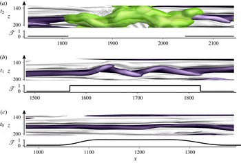
The generation of the target values used in the learning process builds on the database of NB and B streaks. When a spot forms at any position along the length of a streak, the target value indicating whether the streak will break down to turbulence,
 $\mathscr{T}$
, is locally increased over a spatial region comparable to the extent of newly formed spots (see figure 13). For all earlier occurrences of the same streak, streamwise advection is taken into account, and the section is shifted upstream by a distance
 ${\rm\Delta}x=-\bar{u}\;{\rm\Delta}t_{\mathit{spot}}$
, where
 $\bar{u}$
is the local streamwise mean velocity and
 ${\rm\Delta}t_{\mathit{spot}}$
is the time difference to the formation of the spot. In addition, the initially sharp distribution is slightly diffused in the streamwise dimension in order to take into account the increased uncertainty at earlier time instances.
Target value
 $\mathscr{T}$
used in the training of the neural network versus downstream coordinate at three time instances. Regions identified as turbulent by the discrimination scheme are coloured in green.

The adjustment of the weights during the training process requires a large amount of data. In general, the complexity of the ANN scales with the quantity and quality of the available training data. Once the training process is completed, a single prediction of a network with one hidden layer requires just two matrix-vector products (see (3.3)). The associated computational effort is several orders of magnitude lower than that of the solution of the relatively large two-dimensional eigenvalue problems which arise from classical linear stability theory (e.g. Hack & Zaki Reference Hack and Zaki2014a ). Computational efficiency is thus a core advantage of the ANN approach which makes the concept suitable for real-time applications. It is not a substitute, however, to linear analyses which can identify the instability mode and, hence are the foundation for the design of the ANN.
3.2 Prediction in ZPG boundary layer
This section examines the prediction of streak breakdown in ZPG boundary layers. The network is trained using the streak database generated from a time series of 4000 flow fields computed using DNS of bypass transition in boundary layers subject to moderate free-stream turbulence,
 $Tu_{\mathit{FS}}=3\,\%$
. Features are collected from streaks at 18 equidistant cross-planes in the region
 $200<Re_{{\it\theta}}<350$
. The training data set used to adjust the weights of the ANN comprises approximately 30 000 instances of NB streaks and 300 instances of B streaks. The performance of the network is improved by replicating B samples so that the data set used in the actual training procedure contains an equal number of B and NB streaks. The accuracy of the neural network is evaluated using an independent test data set which is obtained from a second DNS time series of the same length and which contains a similar number of approximately 30 000 NB and 300 B streak samples.
The performance of the network is measured in terms of the relative prediction accuracy,
 $$\begin{eqnarray}\mathscr{A}\equiv \frac{1}{M}\mathop{\sum }_{m=1}^{M}1-|\mathscr{P}_{m}-\mathscr{T}_{m}|,\end{eqnarray}$$
where
 $\mathscr{P}_{m}$
is the prediction made by the neural network and
 $\mathscr{T}_{m}$
is the target value of the
 $m$
th sample. The initialization of the weights and the order of the samples during the training process can influence the classification accuracy of the neural network. The following results are thus based on the mean prediction accuracy, defined as the arithmetic average of the predictions of 100 neural networks with individually randomized initial weights and training order.
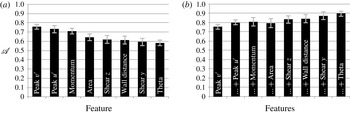
Mean prediction accuracy
 $\mathscr{A}$
of the neural network. Markers indicate two standard deviations. (a) Single input feature. (b) Accumulated input features.

While the data presented in § 2.2 provide a general indication which features are the best identifiers of unstable streaks, the number of all meaningful permutations remains large. A more systematic approach is therefore pursued. First, each of the eight features of the streaks is used as the single input of an ANN with one input neuron. The prediction accuracy computed in this set-up is presented in figure 14(a), where the features have been ranked from high to low
 $\mathscr{A}$
. The results show that the peak wall-normal fluctuation is the most significant feature which yields the best performance. This outcome can be due to the role of the
 $v$
-perturbation in the amplification of streaks via the lift-up process. Furthermore,
 $v^{\prime }$
amplifies appreciably during the secondary instability of the streaks, unlike, for example
 $u^{\prime }$
, which is predominantly set by the primary streak amplitude. As such,
 $s_{v}$
can enable both long-term and short-term forecasts as it can identify streaks that will develop high magnitudes farther downstream as well as streaks that are already distorted by secondary instabilities and will shortly give rise to a turbulent spot. On the other hand, the spanwise as well as the wall-normal shear and the wall distance prove to be relatively peripheral in the identification of unstable streaks when used in isolation.
A second setting seeks to maximize the prediction accuracy by combining the input features. Starting from the single input which yielded the best performance, i.e.
 $s_{v}$
, more features are added in the order of their individual performance. To accommodate the increasing complexity associated with the growing number of inputs, the number of hidden neurons is 64 times the number of input features. Therefore, the first network which only examined a single input included 64 hidden neurons, while the network which examined the entire set of eight input features had 512 neurons in its single hidden layer. The results of this study are presented in figure 14(b). Supplementing the peak wall-normal velocity fluctuation with the streak amplitude yields a moderate improvement of
 $\mathscr{A}$
. Also, addition of the cross-section area does not improve the prediction accuracy in the present set-up. This outcome can be attributed in part to a certain redundancy between the area and the streamwise momentum and peak fluctuation which are already included in the input. The classification accuracy improves when the spanwise shear surrounding the streaks is taken into account. While figure 14(a) showed that the shear alone is a relatively ineffective predictor, its relevance increases when it is considered in conjunction with the preceding features. The result is in line with the recent study by Hack & Zaki (Reference Hack and Zaki2014a
) who demonstrated a clear correlation between the spanwise shear and the growth rate of secondary instabilities. In a separate set of computations, a network based on the features
 $s_{v}$
,
 $s_{u}$
,
 $s_{y}$
,
 $s_{d}$
and
 $s_{{\it\theta}}$
and an increased number of 1280 neurons in the hidden layer achieved an average prediction accuracy of 93 % with a standard deviation of 2.8 %. Overall, these results establish that a feature-based approach can accurately identify streaks that will break down to turbulence.
3.3 Application to FPG and APG boundary layers
An advantageous attribute of neural networks is their capability to generalize, that is to correctly classify unknown and potentially noisy inputs. This generalization ability was, within narrow bounds, already examined in the study of the ZPG boundary layer since the predictions were made on test data that were independent from the data used to adjust the weights of the network. In order to further examine the generalization capabilities, a network trained with data from the ZPG time series is applied to make predictions on breakdown in FPG and APG boundary layers.
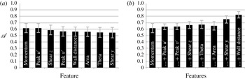
Similar to the ZPG boundary layer, transition in the presence of a moderate favourable pressure gradient is predominantly induced by outer streak instabilities, although the transition process is significantly delayed (see Hack & Zaki Reference Hack and Zaki2014b ). For the FPG case, figure 15(a) shows the prediction accuracy when using only a single input in the training (ZPG data) and testing (FPG data) of the network. In comparison to the earlier results based on test data from ZPG, the prediction accuracy decreases. In particular, the peak wall-normal fluctuation is less predictive in this scenario. The streamwise momentum and the peak streamwise fluctuation both give the best results with an accuracy above 60 %. The combination of all available features leads to a prediction accuracy of 82 %.
Mean prediction accuracy
 $\mathscr{A}$
of the neural network trained for the ZPG case and applied to the FPG case. Markers indicate two standard deviations. (a) Single input feature. (b) Accumulated input features.

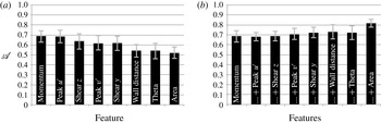
Mean prediction accuracy
 $\mathscr{A}$
of the neural network trained for the ZPG case and applied to the APG case. Markers indicate two standard deviations. (a) Single input feature. (b) Accumulated input features.

Results for the APG case are presented in figure 16. The left panel again ranks the inputs and shows that the use of either the peak streamwise fluctuation or the streamwise momentum leads to an accuracy approximately 65 %. Similar to the FPG case,
 $s_{v}$
is less relevant than in the ZPG boundary layer. When accumulating features, the best accuracy of approximately 82 % is again achieved when all the input variables are included. It should be pointed out that in the moderate adverse-pressure-gradient flow (
 ${\it\beta}_{H}=-0.08$
), breakdown to turbulence is still predominantly initiated by outer streak instabilities situated on top of lifted low-speed streaks (see Nolan & Zaki Reference Nolan and Zaki2013). A study was also conducted for the stronger adverse pressure gradient,
 ${\it\beta}_{H}=-0.14$
. In that case, the best performance obtained by combining all available input features was
 $\mathscr{A}\approx 0.61$
. In this scenario, inner modes which amplify at the local intersection of low-speed and high-speed streaks play an important role. However, the inner instability did not contribute appreciably to the training of the ANN since the training set was obtained from a ZPG configuration where the outer modes are the dominant streak instabilities.
4 Conclusions
In bypass transition to turbulence the laminar boundary layer is laden with streaks with various sizes, amplitudes and orientations. While the streaks have long been speculated to be complicit in the sporadic inception of turbulence spots, only recently was their secondary instability computed in detail. The localized instabilities, however, only affect a very small fraction of streaks among a population of largely innocuous structures. The objectives of the present work were to describe the population of streaks in terms of a low-dimensional set of features; to differentiate streaks that have a high likelihood of breaking down based on these data; and to use this information in the design of an efficient algorithm that can identify the particular ones which are prone to break down to turbulence.
The streaks were identified in time series from DNS, and their attributes were evaluated. Databases of streaks that lead to breakdown to turbulence and of innocuous ones were constructed, and several characteristic parameters were compared. Streaks that induce breakdown to turbulence are generally characterized by higher amplitudes and are located farther away from the wall than the remainder of the population. The latter observation is consistent with their secondary instability being due to an outer instability, and exposure to forcing by free-stream perturbations. Extension of the analysis to adverse- and favourable-pressure-gradient boundary layers showed that the momentum thickness acts as a similarity parameter which collapses various mean streak attributes such as the wall-normal and spanwise shear, the cross-section area and the peak amplitude. Furthermore, the probability density functions of the streak amplitude, peak wall-normal fluctuation, wall-normal and spanwise shear and cross-sectional area also collapse among the various pressure gradients when plotted at the same value of the momentum thickness. Conditional sampling of streaks at the same momentum thickness led to virtually identical velocity perturbation fields for all three mean pressure gradients. In addition, the conditional sampling showed that the unstable streaks tend to be distorted in shape and lifted away from the wall.
The extracted features were used as inputs to an ANN designed to predict the streaks which initiate breakdown to turbulence. The proposed approach is significantly more efficient than the solution of an eigenvalue problem arising from classical linear stability theory. For ZPG boundary layers, the key individual predictors of the streak likelihood to become unstable were its wall-normal and streamwise perturbation velocities. When various inputs are combined, their aggregate led to an accuracy of the forecasts of approximately 90 %. The largest improvement of performance was the addition of the wall-normal height of the streak, which is consistent with the outer nature of its instability. In order to test the generalization capabilities of the method, the neural network trained on the ZPG data was applied to make predictions on the breakdown of streaks in FPG and APG boundary layers. In these cases, the streamwise perturbation and momentum of the streak were the most important indicators of stability. With all the features included, the network still achieved prediction accuracies in excess of 80 %, which demonstrates the flexibility of the approach. Finally, we wish to emphasize that the prediction scheme is not limited to DNS data. The extraction of the streak features from individual cross-flow planes renders the approach compatible with experimental planar measurement techniques, for example two-dimensional particle image velocimetry. In this context, the presented scheme can lead to new avenues for efficient control of transition to turbulence based on accurate real-time identification of unstable streaks.