1 Introduction
The multi-scale nature of plasma dynamics is caused by co-existence of instabilities developing on different scales (Howard et al.
Reference Howard, Holland, White, Greenwald and Candy2014), such as the ion temperature gradient (ITG) instabilities developing on
 $k_{\bot }\unicode[STIX]{x1D70C}_{\text{i}}<1$
with
 $k_{\bot }$
the perpendicular wave number and
 $\unicode[STIX]{x1D70C}_{\text{i}}$
the ion gyro-radius, and the trapped electron modes (TEM) or electron temperature gradient (ETG) modes which are unstable at smaller spatial scales. The multiple scales can also be observed within a single instability (Dominski et al.
Reference Dominski, Brunner, Görler, Jenko, Told and Villard2015). For example, purely electrostatic ITG or TEM modes are basically ion-scale instabilities, which can develop fine radial structures when resolving the kinetic passing electron dynamics at scales shorter than the ion Larmor radius
 $\unicode[STIX]{x1D70C}_{\text{i}}$
. These short-scale structures appear in the electrostatic potential and the species density and temperatures due to the non-adiabatic response of passing electrons near low-order mode rational surfaces and can alter the zonal flows and the level of turbulence transport (Dominski et al.
Reference Dominski, McMillan, Brunner, Merlo, Tran and Villard2017). Another example is the short scales developing when Alfvén eigenmodes, such as the toroidal Alfvén eigenmode, interact with the shear Alfvén continuum (Hasegawa & Chen Reference Hasegawa and Chen1976; Rosenbluth et al.
Reference Rosenbluth, Berk, Van Dam and Lindberg1992; Berk, Mett & Lindberg Reference Berk, Mett and Lindberg1993; Mishchenko, Könies & Hatzky Reference Mishchenko, Könies and Hatzky2011, Reference Mishchenko, Könies and Hatzky2014). Also magnetohydrodynamic (MHD) instabilities, such as the internal kink modes or tearing modes, can develop small structures at resonant flux surfaces if the characteristic inertial scales are smaller than the ion gyro-radius (Porcelli Reference Porcelli1991; Connor, Hastie & Zocco Reference Connor, Hastie and Zocco2012; Mishchenko & Zocco Reference Mishchenko and Zocco2012). Multi-scale simulations are thus obviously required for accurate prediction of magnetic fusion plasma stability and confinement.
Global gyrokinetic particle simulations are routinely used to describe the field fluctuation-driven transport in fusion devices. In particle codes, one discretises the Vlasov equation using the numerical particles (markers) and field equations, such as the quasi-neutrality condition, using finite elements, finite differences or spectral techniques. The gyrokinetic quasi-neutrality condition is given by (Brizard & Hahm Reference Brizard and Hahm2007)
 $$\begin{eqnarray}q_{\text{i}}n_{\text{pol}}=-\int \,\text{d}^{6}Z\unicode[STIX]{x1D6FF}(\boldsymbol{R}+\unicode[STIX]{x1D746}_{\text{i}}-\boldsymbol{x})\frac{q_{\text{i}}^{2}}{B}\frac{\unicode[STIX]{x2202}f_{\text{i}}}{\unicode[STIX]{x2202}\unicode[STIX]{x1D707}}(\unicode[STIX]{x1D719}-\langle \unicode[STIX]{x1D719}\rangle )=\mathop{\sum }_{s}q_{s}n_{1s}\end{eqnarray}$$
with
 $\text{d}^{6}Z=B_{\Vert }^{\ast }\,\text{d}\boldsymbol{R}\,\text{d}v_{\Vert }\,\text{d}\unicode[STIX]{x1D707}\,\text{d}\unicode[STIX]{x1D703}$
,
 $B_{\Vert }^{\ast }$
the Jacobian and where
 $q_{s}$
the particle charge,
 $\boldsymbol{R}$
is the gyro-centre position,
 $\unicode[STIX]{x1D746}_{\text{i}}$
the ion gyro-radius vector,
 $\unicode[STIX]{x1D707}$
the magnetic moment,
 $n_{\text{pol}}$
the polarisation density,
 $f_{s}=f_{0s}+f_{1}$
the full gyrokinetic distribution function,
 $f_{0s}$
the ambient distribution function (usually a Maxwellian),
 $n_{1s}=\int \text{d}^{6}Z\unicode[STIX]{x1D6FF}(\boldsymbol{R}+\unicode[STIX]{x1D746}_{s}-\boldsymbol{x})f_{1s}$
the perturbed gyro-centre density and
 $f_{1s}$
the perturbed part of the gyrokinetic distribution function corresponding to a particle species
 $s=\text{i},\text{e}$
. In (1.1), we have employed the gyro-average of the electrostatic potential
 $\unicode[STIX]{x1D719}$
defined as usual
 $\langle \unicode[STIX]{x1D719}\rangle =\oint \unicode[STIX]{x1D719}(\boldsymbol{R}+\unicode[STIX]{x1D746}(\unicode[STIX]{x1D703}))\,\text{d}\unicode[STIX]{x1D703}/(2\unicode[STIX]{x03C0})$
. Usually, the polarisation density is considered in the linear approximation replacing full
 $f_{\text{i}}$
with the ambient
 $f_{0\text{i}}$
in (1.1). This approximation is related to the gyro-fluid Boussinesq approximation (Yu, Krasheninnikov & Guzdar Reference Yu, Krasheninnikov and Guzdar2006; Angus & Umansky Reference Angus and Umansky2014; Wiesenberger, Madsen & Kendl Reference Wiesenberger, Madsen and Kendl2014; Kendl Reference Kendl2015) and can fail for edge plasma conditions.
Note that the polarisation density appearing on the left-hand side of the quasi-neutrality equation is formulated in terms of a phase-space integral. This complicates a numerical treatment of the polarisation density in global codes. In a local approximation, the linearised polarisation density is
 $$\begin{eqnarray}n_{\text{pol}}(\boldsymbol{k})=\frac{n_{0}q_{\text{i}}}{T_{\text{i}}}[1-\unicode[STIX]{x1D6E4}_{0}(k_{\bot }\unicode[STIX]{x1D70C}_{\text{i}})]\unicode[STIX]{x1D719}(\boldsymbol{k}),\quad \unicode[STIX]{x1D6E4}_{0}(x)=I_{0}(x^{2})\exp (-x^{2})\end{eqnarray}$$
with
 $\boldsymbol{k}$
the wave vector of the field perturbation and
 $I_{0}(x)$
the Bessel function of the first kind. Taking into account that
 $\unicode[STIX]{x1D6E4}_{0}(x)\approx 1-x^{2}$
for small
 $x$
, one can write the polarisation density in the long-wavelength approximation
 $k_{\bot }\unicode[STIX]{x1D70C}_{\text{i}}\ll 1$
as
 $$\begin{eqnarray}n_{\text{pol}}(\boldsymbol{k})\approx \frac{n_{0}q_{\text{i}}}{T_{\text{i}}}(k_{\bot }\unicode[STIX]{x1D70C}_{\text{i}})^{2}\unicode[STIX]{x1D719}(\boldsymbol{k}).\end{eqnarray}$$
Alternatively, the Padé approximation
 $\unicode[STIX]{x1D6E4}_{0}(x)\approx (1+x^{2})^{-1}$
can be used at arbitrarily large
 $k_{\bot }\unicode[STIX]{x1D70C}_{\text{i}}$
leading to the approximate polarisation density:
 $$\begin{eqnarray}n_{\text{pol}}(\boldsymbol{k})=\frac{n_{0}q_{\text{i}}}{T_{\text{i}}}[1-\unicode[STIX]{x1D6E4}_{0}(k_{\bot }\unicode[STIX]{x1D70C}_{\text{i}})]\unicode[STIX]{x1D719}(\boldsymbol{k})\approx \frac{n_{0}q_{\text{i}}}{T_{\text{i}}}\frac{(k_{\bot }\unicode[STIX]{x1D70C}_{\text{i}})^{2}}{1+(k_{\bot }\unicode[STIX]{x1D70C}_{\text{i}})^{2}}\unicode[STIX]{x1D719}(\boldsymbol{k}).\end{eqnarray}$$
Globally, one can replace
 $k_{\bot }^{2}$
with
 $-\unicode[STIX]{x1D6FB}_{\bot }^{2}$
to obtain the self-adjoint long-wavelength approximation:
 $$\begin{eqnarray}-\unicode[STIX]{x1D735}\boldsymbol{\cdot }\left[\frac{q_{\text{i}}n_{0}}{T_{\text{i}}}\unicode[STIX]{x1D70C}_{\text{i}}^{2}\unicode[STIX]{x1D735}_{\bot }\unicode[STIX]{x1D719}\right]=(n_{1\text{i}}-n_{1\text{e}}).\end{eqnarray}$$
This equation can also be obtained without invoking the Fourier transformation by a straightforward Taylor expansion at small gyro-radius
 $|\unicode[STIX]{x1D746}_{\text{i}}|\ll |\boldsymbol{R}|$
of the global polarisation density, equation (1.1). Similarly, the Padé approximation is
 $$\begin{eqnarray}-\unicode[STIX]{x1D735}\boldsymbol{\cdot }\left[\frac{q_{\text{i}}n_{0}}{T_{\text{i}}}\unicode[STIX]{x1D70C}_{\text{i}}^{2}\unicode[STIX]{x1D735}_{\bot }\unicode[STIX]{x1D719}\right]=(n_{1\text{i}}-n_{1\text{e}})-\unicode[STIX]{x1D735}\boldsymbol{\cdot }[\unicode[STIX]{x1D70C}_{\text{i}}^{2}\unicode[STIX]{x1D735}_{\bot }(n_{1\text{i}}-n_{1\text{e}})].\end{eqnarray}$$
Note that the right-hand side is different for the Padé approximation, equation (1.6), compared with the long-wavelength approximation, equation (1.5). This difference corresponds to
 $1+(k_{\bot }\unicode[STIX]{x1D70C}_{\text{i}})^{2}$
appearing in the denominator on the right-hand side of (1.4). The long-wavelength approximation becomes poor at the scales comparable to the ion gyro-radius. In contrast, the Padé approximation is usually quite good in practice but it is still an approximation. It is desirable to have a direct approach to the global polarisation density without invoking any simplifications. For this purpose, an arbitrarily short-wavelength solver, directly discretising the global polarisation density, equation (1.1), has been introduced in Lin & Lee (Reference Lin and Lee1995) and Mishchenko, Könies & Hatzky (Reference Mishchenko, Könies and Hatzky2005) where it was called the ‘generalised solver’. The phase-space integral for computing the polarisation drift contribution to the quasi-neutrality equation was carried out with a Monte Carlo-type integration. The corresponding solver has been implemented in the GYGLES code and employed to study the short-wavelength ion temperature gradient modes (Mishchenko, Hatzky & Könies Reference Mishchenko, Hatzky and Könies2006), bulk plasma effects on the toroidal Alfvén eigenmodes including their interaction with the shear-Alfvén-wave continuum (Mishchenko et al.
Reference Mishchenko, Könies and Hatzky2011, Reference Mishchenko, Könies and Hatzky2014), and internal kink modes (Mishchenko & Zocco Reference Mishchenko and Zocco2012). Recently, a similar approach was implemented in the ORB5 code (Dominski et al.
Reference Dominski, McMillan, Brunner, Merlo, Tran and Villard2017) and used to study effects of the non-adiabatic electron dynamics at resonant flux surfaces on the ITG and TEM instabilities in tokamak geometry. In this latter reference, the phase-space integral corresponding to the polarisation density is replaced by quadratures over an Eulerian grid and analytic integration.
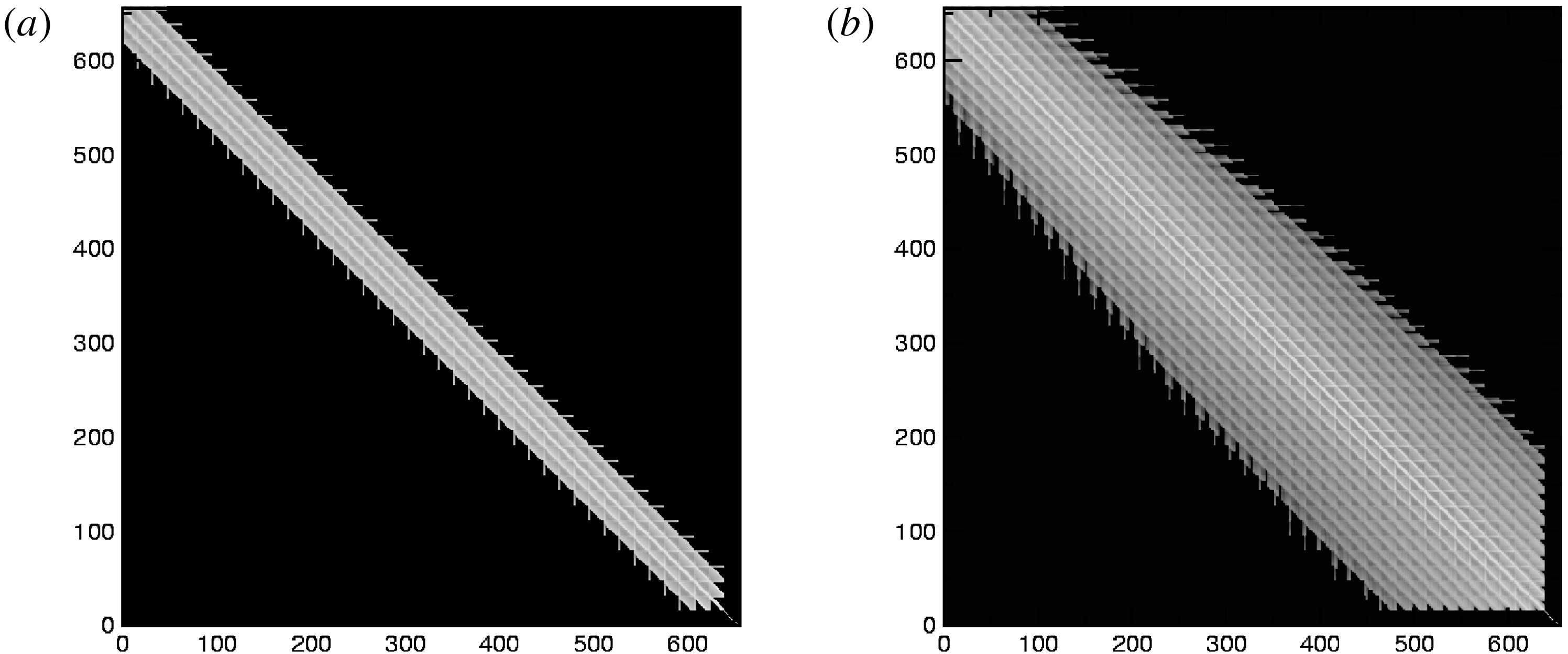
The price to pay for the arbitrarily short-wavelength solver is the explicitly non-local nature of the matrix representing the polarisation density. Generally, this matrix corresponds to an integral operator, equation (1.1), and is not sparse (Mishchenko et al. Reference Mishchenko, Hatzky and Könies2006; Dominski et al. Reference Dominski, McMillan, Brunner, Merlo, Tran and Villard2017). The resulting computer memory footprint can be quite substantial. In contrast, both the long-wavelength and Padé approximations are formulated in terms of differential operators leading to much smaller sparse band matrices, see figure 1. In Dominski et al. (Reference Dominski, McMillan, Brunner, Merlo, Tran and Villard2017), this problem has been mitigated by a field-aligned Fourier solver (McMillan et al. Reference McMillan, Jolliet, Bottino, Angelino, Tran and Villard2010). However, the Fourier transform of the general polarisation-density operator in itself is non-trivial if computed using the Monte Carlo approach (Mishchenko et al. Reference Mishchenko, Könies and Hatzky2005). In Dominski et al. (Reference Dominski, McMillan, Brunner, Merlo, Tran and Villard2017), an Eulerian grid has been used to circumvent this. Another problem, related specifically to the Monte Carlo computation of the polarisation-density matrix, is the associate particle noise. It may lead to difficulties in the matrix inversion using Cholesky decomposition since the eigenvalues of this matrix close to zero may become ‘numerically negative’ due to the statistical inaccuracies. This type of behaviour has been observed both with the GYGLES (Mishchenko et al. Reference Mishchenko, Könies and Hatzky2005) and with the ORB5 (Dominski et al. Reference Dominski, McMillan, Brunner, Merlo, Tran and Villard2017) codes. In practice, one can circumvent this by using the LDL decomposition technique, but it is of course desirable to resolve such a problem.
(a) Polarisation-density matrix structure corresponding to the long-wavelength approximation. (b) Arbitrarily short-wavelength matrix. The number of non-zero elements increases strongly with the spatial resolution. Figure taken from Mishchenko et al. (Reference Mishchenko, Hatzky and Könies2006).

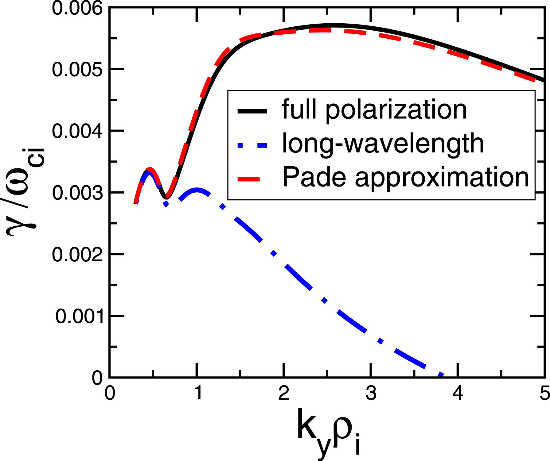
Comparison of the ITG growth rates computed using the full polarisation density, the Padé approximation and the long-wavelength approximation. The local dispersion relation in slab geometry (Mishchenko et al. Reference Mishchenko, Zocco, Helander and Könies2018) has been solved numerically.

All these technical difficulties provide a motivation for an alternative iterative formulation of the arbitrarily short-wavelength solver based on the observation that the Padé approximation is usually quite good in practice, especially in the local approximation, shown in figure 2. Therefore, one can use the deviation of the Padé approximation from the exact polarisation density, computed in some norm, as a small parameter in order to construct an iterative scheme. In addition, we will see that the iterative formulation can be used to relax the linear (Boussinesq) approximation of the polarisation density. A similar scheme has been earlier considered for nonlinear polarisation density by Idomura (Reference Idomura2012) with the focus on momentum transport. Physically, the nonlinearity in the polarisation density may be of importance since it represents the dynamic part of the plasma inertia changing as a consequence of the perturbed plasma motion. This could, for example, modify the shear Alfvén wave whose frequency is determined by the plasma inertia.
The structure of the paper is as follows. In § 2, we discuss the discretisation of the quasi-neutrality equation, following (Mishchenko et al. Reference Mishchenko, Könies and Hatzky2005). The iterative approach is described in § 3. It is applied to the linear polarisation density in § 4 and extended to the nonlinear case in § 5. We make our conclusions in § 6.
2 Discretisation of the linearised polarisation density
In the GYGLES code, the polarisation density is discretised with finite elements (tensor products of B splines) employing the phase factor transformation (Fivaz et al. Reference Fivaz, Brunner, de Ridder, Sauter, Tran, Vaclavik, Villard and Appert1998):
 $$\begin{eqnarray}\unicode[STIX]{x1D719}(\boldsymbol{x})=\hat{\unicode[STIX]{x1D719}}(\boldsymbol{x})\text{e}^{\text{i}S(\boldsymbol{x})},\quad f_{1a}(\boldsymbol{R})=\hat{f}_{1a}(\boldsymbol{R})\text{e}^{\text{i}S(\boldsymbol{R})},\quad S=m_{0}\unicode[STIX]{x1D703}-n_{0}\unicode[STIX]{x1D711}.\end{eqnarray}$$
Here,
 $S$
is the phase factor,
 $\unicode[STIX]{x1D703}$
is the poloidal angle,
 $\unicode[STIX]{x1D711}$
is the toroidal angle,
 $m_{0}$
and
 $n_{0}$
are properly chosen poloidal and toroidal wavenumbers. The phase-factor transformed field
 $\hat{\unicode[STIX]{x1D719}}$
is discretised as
 $\hat{\unicode[STIX]{x1D719}}(\boldsymbol{x},t)=\sum _{k}\unicode[STIX]{x1D719}_{k}(t)\unicode[STIX]{x1D6EC}_{k}(\boldsymbol{x})$
with
 $\unicode[STIX]{x1D6EC}_{k}$
the finite elements (tensor products of B splines) and
 $\unicode[STIX]{x1D719}_{k}$
the expansion coefficients. For the phase-factor transformed distribution function, we write
 $\hat{f}_{1a}(Z,t)=\sum _{\unicode[STIX]{x1D708}}w_{\unicode[STIX]{x1D708}}\unicode[STIX]{x1D6FF}(Z-Z_{\unicode[STIX]{x1D708}}(t))$
with
 $w_{\unicode[STIX]{x1D708}}$
the marker weight and
 $Z_{\unicode[STIX]{x1D708}}(t)$
the marker position in phase space. Introducing the phase-factor notation
 $$\begin{eqnarray}\unicode[STIX]{x1D6E5}_{\text{A}}=\exp [\text{i}S(\boldsymbol{R})-\text{i}S(\boldsymbol{R}+\unicode[STIX]{x1D746})],\quad \unicode[STIX]{x1D6E5}_{\text{F}}=\exp [\text{i}S(\boldsymbol{R}+\unicode[STIX]{x1D746})-\text{i}S(\boldsymbol{R})]\end{eqnarray}$$
we can write the quasi-neutrality condition (1.1) in matrix form:
 $$\begin{eqnarray}\mathop{\sum }_{l}G_{kl}\unicode[STIX]{x1D719}_{l}=b_{k},\quad b_{k}=\mathop{\sum }_{s=\text{i},\text{e}}q_{s}\mathop{\sum }_{\unicode[STIX]{x1D708}=1}^{N_{\text{p}}}w_{s\unicode[STIX]{x1D708}}\langle \unicode[STIX]{x1D6EC}_{k}\unicode[STIX]{x1D6E5}_{\text{A}}\rangle .\end{eqnarray}$$
The linear polarisation matrix is computed using the Monte Carlo approach
 $$\begin{eqnarray}f_{0\text{i}}=\mathop{\sum }_{\unicode[STIX]{x1D702}=1}^{{\tilde{N}}_{\text{p}}}f_{0\text{i}\unicode[STIX]{x1D702}}\unicode[STIX]{x1D701}_{\text{i}\unicode[STIX]{x1D702}}\unicode[STIX]{x1D6FF}(Z-Z_{\unicode[STIX]{x1D702}}),\quad G_{kl}=q_{\text{i}}\mathop{\sum }_{\unicode[STIX]{x1D702}=1}^{{\tilde{N}}_{\text{p}}}\frac{f_{0\text{i}\unicode[STIX]{x1D702}}\unicode[STIX]{x1D701}_{\text{i}\unicode[STIX]{x1D702}}}{T_{\text{i}\unicode[STIX]{x1D702}}}(\langle \unicode[STIX]{x1D6EC}_{k}\unicode[STIX]{x1D6EC}_{l}\rangle -\langle \unicode[STIX]{x1D6EC}_{k}\unicode[STIX]{x1D6E5}_{\text{A}}\rangle \langle \unicode[STIX]{x1D6EC}_{l}\unicode[STIX]{x1D6E5}_{\text{F}}\rangle )\end{eqnarray}$$
with the finite elements and the phase factors computed at the gyro-points corresponding to the
 $\unicode[STIX]{x1D702}$
th ‘polarisation-density particle’ with the phase-space volume
 $\unicode[STIX]{x1D701}_{\text{i}\unicode[STIX]{x1D702}}$
. Note that
 $\unicode[STIX]{x2202}f_{0\text{i}}/\unicode[STIX]{x2202}\unicode[STIX]{x1D707}$
appearing in the polarisation density has been computed for the linear polarisation density analytically assuming
 $f_{0\text{i}}$
to be a Maxwellian. For more details, see Mishchenko et al. (Reference Mishchenko, Könies and Hatzky2005).
3 Iterative scheme for generalised solver
The most general matrix form for the quasi-neutrality equation
 $$\begin{eqnarray}\mathop{\sum }_{l}(\bar{L}_{kl}+G_{kl})\unicode[STIX]{x1D719}_{l}=b_{k}\end{eqnarray}$$
corresponds to the adiabatic-electron approximation:
 $$\begin{eqnarray}\frac{q_{\text{e}}^{2}n_{0}}{T_{\text{e}}}(\unicode[STIX]{x1D719}-\bar{\unicode[STIX]{x1D719}})-\int \,\text{d}^{6}Z\unicode[STIX]{x1D6FF}(\boldsymbol{R}+\unicode[STIX]{x1D746}_{\text{i}}-\boldsymbol{x})\frac{q_{\text{i}}^{2}}{B}\frac{\unicode[STIX]{x2202}f_{0\text{i}}}{\unicode[STIX]{x2202}\unicode[STIX]{x1D707}}\widetilde{\unicode[STIX]{x1D719}}=q_{\text{i}}\int \,\text{d}^{6}Z\unicode[STIX]{x1D6FF}(\boldsymbol{R}+\unicode[STIX]{x1D746}_{\text{i}}-\boldsymbol{x})f_{1\text{i}}.\end{eqnarray}$$
Here,
 $\bar{\unicode[STIX]{x1D719}}$
is the flux-surface average of the electrostatic potential,
 $\langle \unicode[STIX]{x1D719}\rangle$
is its gyro-average and
 $\widetilde{\unicode[STIX]{x1D719}}=\unicode[STIX]{x1D719}-\langle \unicode[STIX]{x1D719}\rangle$
. The numerical computation of the polarisation-density phase-space integral can be optimised if the distribution function
 $f_{0\text{i}}$
is known analytically, e.g. it is a Maxwellian. Then, one can use importance sampling for the ‘polarisation-density particles’ used to compute this integral. The numerical distribution of these particle can be optimised for the distribution function
 $f_{0\text{i}}$
, the magnetic field
 $B$
, etc.
In matrix form, equation (3.1), the matrix
 $\bar{L}_{kl}$
corresponds to the adiabatic-electron term:
 $$\begin{eqnarray}\bar{L}_{kl}=\int \,\text{d}^{3}x\frac{q_{\text{e}}^{2}n_{0}}{T_{\text{e}}}[\unicode[STIX]{x1D6EC}_{k}(\boldsymbol{x})\unicode[STIX]{x1D6EC}_{l}(\boldsymbol{x})-\bar{\unicode[STIX]{x1D6EC}}_{k}\bar{\unicode[STIX]{x1D6EC}}_{l}]\end{eqnarray}$$
with
 $\bar{\unicode[STIX]{x1D6EC}}_{k}$
the flux-surface average of the finite element
 $\unicode[STIX]{x1D6EC}_{k}(\boldsymbol{x})$
, the matrix
 $G_{kl}$
is the arbitrarily short-wavelength polarisation-density matrix, given by (2.4),
 $b_{k}$
is the charge-assignment vector, defined in (2.3), and
 $\unicode[STIX]{x1D719}_{l}$
is the vector of the B spline coefficients. The exact arbitrarily short-wavelength polarisation-density matrix can be Padé approximated as follows:
 $$\begin{eqnarray}G\approx {\hat{G}}=(I+\hat{L}M^{-1})^{-1}L,\end{eqnarray}$$
where
 $I$
is the identity matrix,
 $M$
is the mass matrix,
 $L$
is the long-wavelength Poisson matrix and
 $\hat{L}$
is the Poisson matrix, corresponding to
 $k_{\bot }^{2}\unicode[STIX]{x1D70C}_{\text{i}}^{2}$
in the local limit, defined as
 $$\begin{eqnarray}M_{kl}=\int \,\text{d}^{3}x\unicode[STIX]{x1D6EC}_{k}(\boldsymbol{x})\unicode[STIX]{x1D6EC}_{l}(\boldsymbol{x}),\quad L_{kl}=\int \,\text{d}^{3}x\frac{m_{\text{i}}n_{0}}{B^{2}}\unicode[STIX]{x1D735}_{\bot }^{(+)}\unicode[STIX]{x1D6EC}_{k}\unicode[STIX]{x1D735}_{\bot }^{(-)}\unicode[STIX]{x1D6EC}_{l}\end{eqnarray}$$
 $$\begin{eqnarray}\hat{L}_{kl}=\int \,\text{d}^{3}x\frac{m_{\text{i}}T_{\text{i}}}{q_{\text{i}}B^{2}}\unicode[STIX]{x1D735}_{\bot }^{(+)}\unicode[STIX]{x1D6EC}_{k}\unicode[STIX]{x1D735}_{\bot }^{(-)}\unicode[STIX]{x1D6EC}_{l},\quad \unicode[STIX]{x1D735}^{(\pm )}=\unicode[STIX]{x1D735}\pm \text{i}\unicode[STIX]{x1D735}S.\end{eqnarray}$$
To derive an iterative generalised solver, we add a zero to the right-hand side of the arbitrarily short-wavelength quasi-neutrality equation (3.1):
 $$\begin{eqnarray}\bar{L}\unicode[STIX]{x1D719}+G\unicode[STIX]{x1D719}=b+({\hat{G}}-{\hat{G}})\unicode[STIX]{x1D719}\end{eqnarray}$$
with the matrix indices skipped for simplicity. Rearranging the terms, we obtain:
 $$\begin{eqnarray}(\bar{L}+{\hat{G}})\unicode[STIX]{x1D719}=b+({\hat{G}}-G)\unicode[STIX]{x1D719}\end{eqnarray}$$
with
 $\Vert {\hat{G}}-G\Vert =O(\unicode[STIX]{x1D700})$
where the small parameter
 $\unicode[STIX]{x1D700}$
characterises how good the Padé formula approximates the exact polarisation density; the approximation is good if the spectral radius
 $\unicode[STIX]{x1D70C}(G-{\hat{G}})<1$
. Substituting the expression for
 ${\hat{G}}$
, equation (3.4), we obtain:
 $$\begin{eqnarray}[\bar{L}+(I+\hat{L}M^{-1})^{-1}L]\unicode[STIX]{x1D719}=b+[(I+\hat{L}M^{-1})^{-1}L-G]\unicode[STIX]{x1D719}.\end{eqnarray}$$
Left-multiplying this equation with
 $(I+\hat{L}M^{-1})$
, results in
 $$\begin{eqnarray}[\bar{L}+(\hat{L}M^{-1})\bar{L}+L]\unicode[STIX]{x1D719}=b+(\hat{L}M^{-1})b+[L-G-(\hat{L}M^{-1})G]\unicode[STIX]{x1D719}.\end{eqnarray}$$
This equation is the basis for the iterative solution. Expanding the electrostatic potential in powers of the small parameter
 $\unicode[STIX]{x1D719}=\unicode[STIX]{x1D719}_{0}+\unicode[STIX]{x1D700}\unicode[STIX]{x1D719}_{1}+\unicode[STIX]{x1D700}^{2}\unicode[STIX]{x1D719}_{2}+\cdots \,$
, we obtain
 $$\begin{eqnarray}\displaystyle & [\bar{L}+(\hat{L}M^{-1})\bar{L}+L]\unicode[STIX]{x1D719}_{0}=b+(\hat{L}M^{-1})b & \displaystyle\end{eqnarray}$$
 $$\begin{eqnarray}\displaystyle & [\bar{L}+(\hat{L}M^{-1})\bar{L}+L]\unicode[STIX]{x1D719}_{1}=[L-G-(\hat{L}M^{-1})G]\unicode[STIX]{x1D719}_{0} & \displaystyle\end{eqnarray}$$
 $$\begin{eqnarray}\displaystyle & [\bar{L}+(\hat{L}M^{-1})\bar{L}+L]\unicode[STIX]{x1D719}_{2}=[L-G-(\hat{L}M^{-1})G]\unicode[STIX]{x1D719}_{1}. & \displaystyle\end{eqnarray}$$
Introducing the following notation for the partial sums
 $$\begin{eqnarray}\hat{\unicode[STIX]{x1D719}}_{0}=\unicode[STIX]{x1D719}_{0},\quad \hat{\unicode[STIX]{x1D719}}_{1}=\unicode[STIX]{x1D719}_{0}+\unicode[STIX]{x1D719}_{1},\quad \hat{\unicode[STIX]{x1D719}}_{2}=\unicode[STIX]{x1D719}_{0}+\unicode[STIX]{x1D719}_{1}+\unicode[STIX]{x1D719}_{2},\ldots ,\end{eqnarray}$$
we can write the iterative scheme in terms of
 $\hat{\unicode[STIX]{x1D719}}$
as follows:
 $$\begin{eqnarray}\displaystyle & [\bar{L}+(\hat{L}M^{-1})\bar{L}+L]\hat{\unicode[STIX]{x1D719}}_{0}=b+(\hat{L}M^{-1})b & \displaystyle\end{eqnarray}$$
 $$\begin{eqnarray}\displaystyle & [\bar{L}+(\hat{L}M^{-1})\bar{L}+L]\hat{\unicode[STIX]{x1D719}}_{n}=b+(\hat{L}M^{-1})b+[L-G-(\hat{L}M^{-1})G]\hat{\unicode[STIX]{x1D719}}_{n-1},\quad n\geqslant 1.\qquad & \displaystyle\end{eqnarray}$$
Assuming
 $\unicode[STIX]{x1D719}=\lim _{n\rightarrow \infty }\hat{\unicode[STIX]{x1D719}}_{n}$
, we can rewrite (3.16) as
 $$\begin{eqnarray}[\bar{L}+(\hat{L}M^{-1})\bar{L}+L]\unicode[STIX]{x1D719}=b+(\hat{L}M^{-1})b+[L-G-(\hat{L}M^{-1})G]\unicode[STIX]{x1D719}.\end{eqnarray}$$
This equation can be further transformed to
 $$\begin{eqnarray}(I+\hat{L}M^{-1})(\bar{L}+G)\unicode[STIX]{x1D719}=(I+\hat{L}M^{-1})b\end{eqnarray}$$
which is satisfied for the exact quasi-neutrality equation
 $(\bar{L}+G)\unicode[STIX]{x1D719}=b$
, see (3.1). This provides a consistency test for the iterative scheme derived here.
Note that the matrix
 $(\hat{L}M^{-1})\bar{L}$
appearing on the left-hand side of the quasi-neutrality equation in the adiabatic-electron approximation, see for example (3.16), is actually non-Hermitian since the matrices
 $\hat{L}$
and
 $M^{-1}$
do not commute. In the code, this issue is resolved by writing the strong form of the adiabatic-electron approximation of the quasi-neutrality equation in a way preserving the self-adjoint structure:
 $$\begin{eqnarray}-\unicode[STIX]{x1D735}\boldsymbol{\cdot }\left[\left(\frac{m_{\text{i}}n_{0}}{B^{2}}+\frac{q_{\text{e}}^{2}T_{\text{i}}}{q_{\text{i}}^{2}T_{\text{e}}}\frac{m_{\text{i}}n_{0}}{B^{2}}\right)\unicode[STIX]{x1D735}_{\bot }\unicode[STIX]{x1D719}\right]+\frac{q_{\text{e}}^{2}n_{0}}{T_{\text{e}}}\unicode[STIX]{x1D719}=q_{\text{i}}n_{1\text{i}}-\unicode[STIX]{x1D735}\boldsymbol{\cdot }\left(\frac{m_{\text{i}}T_{\text{i}}}{q_{\text{i}}B^{2}}\unicode[STIX]{x1D735}_{\bot }n_{1\text{i}}\right).\end{eqnarray}$$
In the weak form it implies the following replacement on the left-hand side of the quasi-neutrality equation in the adiabatic-electron approximation:
 $$\begin{eqnarray}[(\hat{L}M^{-1})\bar{L}]_{kl}\longrightarrow \int \,\text{d}^{3}x\frac{q_{\text{e}}^{2}T_{\text{i}}}{q_{\text{i}}^{2}T_{\text{e}}}\frac{m_{\text{i}}n_{0}}{B^{2}}\unicode[STIX]{x1D735}_{\bot }^{(+)}\unicode[STIX]{x1D6EC}_{k}\unicode[STIX]{x1D735}_{\bot }^{(-)}\unicode[STIX]{x1D6EC}_{l}.\end{eqnarray}$$
Note that this replacement must be applied always when the Padé approximation is used. It is not a specific feature of the iterative arbitrarily short-wavelength solver described in this paper. Non-Hermiticity of the matrix
 $\hat{L}M^{-1}$
appearing on the right-hand side of the quasi-neutrality equation does not cause any problems for the solver.
4 Linear polarisation density
In the iterative scheme (3.16), the products
 $G\unicode[STIX]{x1D719}_{n}$
have to be computed. This can be done using the actual matrix
 $G$
, equation (2.4), pre-computed and stored at the beginning of the simulation. This ‘direct-matrix’ approach requires substantial memory consumption and is not suited for the nonlinear polarisation density. An alternative is to use the ‘matrix-free’ formulation with the ‘polarisation vector’ defined as
 $$\begin{eqnarray}g_{k}^{(n)}=G\unicode[STIX]{x1D719}_{n}=\mathop{\sum }_{\unicode[STIX]{x1D708}=1}^{N_{\text{p}}}\frac{q}{T}f_{0}(Z_{\unicode[STIX]{x1D708}})\unicode[STIX]{x1D701}_{\unicode[STIX]{x1D708}}(\langle \unicode[STIX]{x1D6EC}_{k}\unicode[STIX]{x1D719}_{n}\rangle -\langle \unicode[STIX]{x1D6EC}_{k}\unicode[STIX]{x1D6E5}_{\text{A}}\rangle \langle \unicode[STIX]{x1D719}_{n}\unicode[STIX]{x1D6E5}_{\text{F}}\rangle ).\end{eqnarray}$$
The finite elements, the phase factors, and the fields are computed at the gyro-point
 $\boldsymbol{R}_{\unicode[STIX]{x1D708}}+\unicode[STIX]{x1D746}_{\unicode[STIX]{x1D708}}$
associated with the
 $\unicode[STIX]{x1D708}$
th polarisation-density particle. Note that in the sums such as (4.1), the same markers moving along the gyrokinetic orbits can be used for the matrix computation as in the charge assignment, opening a way for the matrix-free nonlinear polarisation density treatment. In this case, one would have to handle numerically the
 $\unicode[STIX]{x1D707}$
-derivative of a distribution function unknown analytically and discretised with the markers, see (1.1). We will give a solution of this problem in the next section. The polarisation vector
 $g_{n}$
has to be computed using particles on every iterative step, equation (3.16), it has to be multiplied with the matrix
 $I+\hat{L}M^{-1}$
(the same operation has to be performed on the charge-assignment vector
 $b$
), and combined with the correction vector
 $L\hat{\unicode[STIX]{x1D719}}_{n}$
which can be computed on the grid without invoking the markers. Note that all the matrices to be inverted in the iterative formulation of the solver are computed on the grid and therefore free of the statistical errors which could otherwise break the symmetry of the system in an uncontrolled way, in contrast to the direct solver where the noisy Monte Carlo matrix appears on the left-hand side and has to be inverted. In the iterative formulation, the noisy part is moved to the right-hand side where it can be treated on the same footing as the charge assignment, also prone to statistical errors, using the same noise-control techniques. A simple Poisson solver is sufficient to address (3.16) for all iterations needed. This means that the usual, for example Dirichlet, boundary conditions can, in principle, be used and the Fourier matrix implementation (McMillan et al.
Reference McMillan, Jolliet, Bottino, Angelino, Tran and Villard2010) is straightforward. The simple handling of the boundary conditions for the iterative solver is a practical convenience while its rigorous justification remains beyond the scope of this paper. A detailed discussion on the subtleties of the boundary conditions for the arbitrarily short-wavelength solver can be found in Dominski et al. (Reference Dominski, McMillan, Brunner, Merlo, Tran and Villard2017). Note that the differential operator on the left-hand side of (3.16) leads to Hermitian and positive-definite matrices, sharing these properties with the arbitrarily short-wavelength polarisation-density matrix, equation (2.4). For the adiabatic-electron approximation, equation (3.20) must be used.
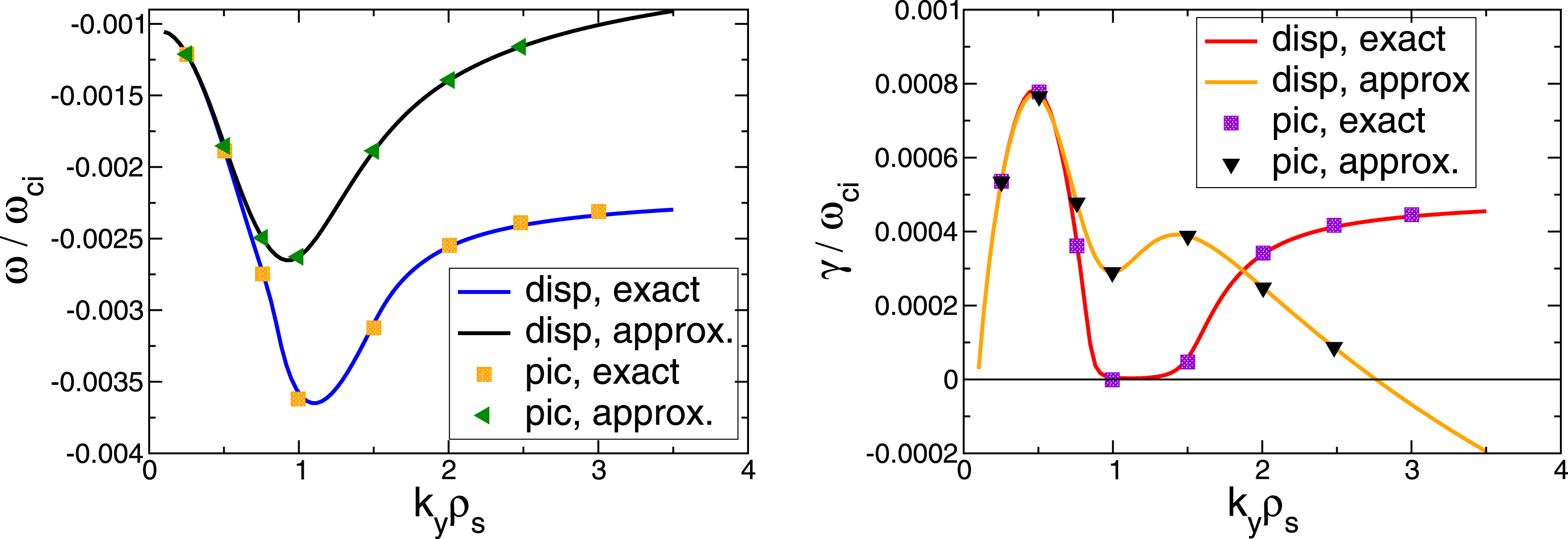
In figure 3, we prove that the iterative solver proposed here gives the right result. Here, the frequency and the growth rate of the ITG mode in shearless slab geometry resulting from GYGLES simulations are compared with the numerical solution of the local dispersion relation (Mishchenko et al.
Reference Mishchenko, Zocco, Helander and Könies2018) for both the iterative arbitrarily short-wavelength solver and the long-wavelength approximation. The ion and electron temperature gradient lengths
 $\unicode[STIX]{x1D70C}_{s}/L_{\text{Ti}}=\unicode[STIX]{x1D70C}_{s}/L_{\text{Te}}=0.0223$
with
 $\unicode[STIX]{x1D70C}_{s}=\sqrt{m_{\text{i}}T_{\text{e}}}/(q_{\text{i}}B)$
, the density profile is flat. We choose the mode structure in such a way that
 $k_{\bot }\approx k_{y}$
where
 $k_{y}$
is the ‘poloidal’ wavenumber. For more details on similar simulations using the direct (non-iterative) arbitrarily short-wavelength solver, see Mishchenko et al. (Reference Mishchenko, Könies and Hatzky2005). In figure 3, one sees that the agreement between the dispersion relation solution and the results of the iterative arbitrarily short-wavelength solver is very good. This result verifies the iterative approach, described in this section.
The frequency and the growth rate of the ITG mode in shearless slab geometry resulting from the gyrokinetic particle-in-cell (PIC) simulations plotted as a function of
 $k_{\bot }\unicode[STIX]{x1D70C}_{s}$
and compared to the numerical solution of the dispersion relation (Mishchenko et al.
Reference Mishchenko, Zocco, Helander and Könies2018). Both the iterative arbitrarily short-wavelength results and the long-wavelength approximation (corresponding to ‘disp, approx’ and ‘pic, approx’ in the legend) results are shown.

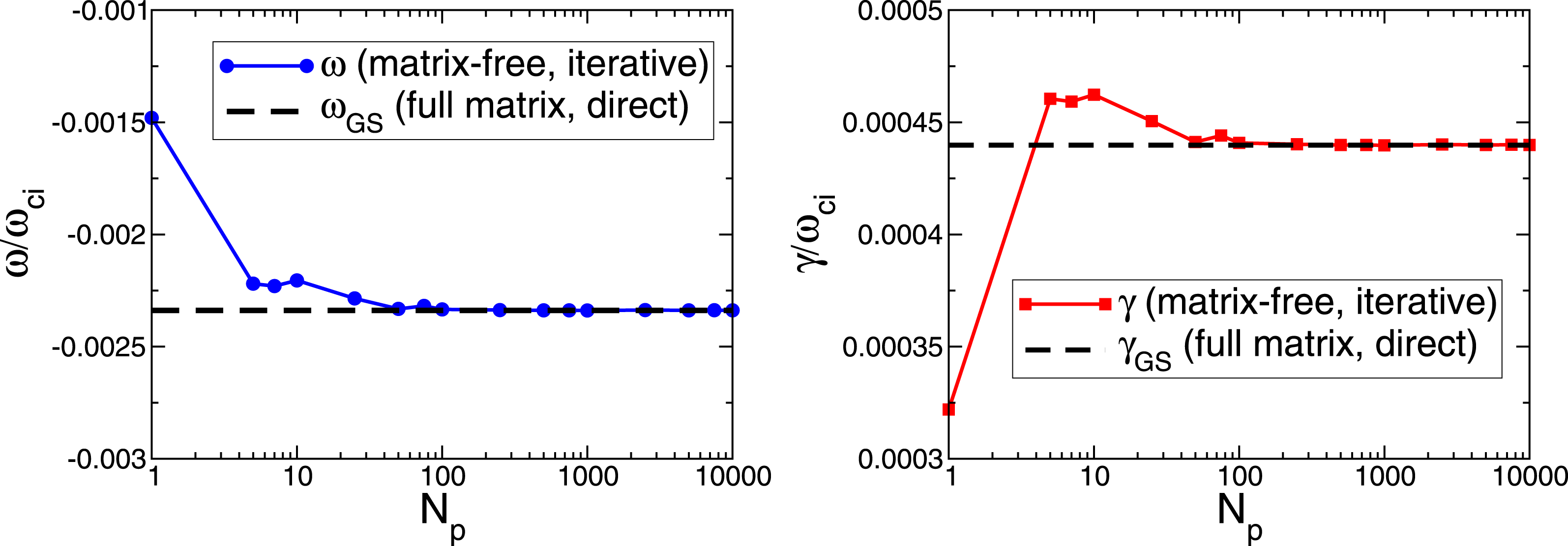
The frequency and the growth rate obtained with the iterative arbitrarily short-wavelength solver (3.16) plotted as a function of the number of the ‘polarisation-density particles’ used in (3.16). The iterative solver (3.16) is compared to the direct solver (Mishchenko et al.
Reference Mishchenko, Könies and Hatzky2005). The ITG mode in shearless slab geometry is considered for
 $k_{y}\unicode[STIX]{x1D70C}_{s}=3$
, see figure 3. Already a small number of the particles gives a good agreement with the dispersion relation (Mishchenko et al.
Reference Mishchenko, Zocco, Helander and Könies2018) demonstrating the efficiency of the iterative solver.

In figure 4, we show a convergence study with respect to the number of the polarisation-density particles used to compute the sum in (4.1). Here, we consider the ITG mode in shearless slab geometry corresponding to
 $k_{y}\unicode[STIX]{x1D70C}_{s}=3$
in figure 3. One sees that already a small number of polarisation-density particles gives a good agreement with the dispersion relation. This makes our iterative solver very efficient in terms of computation time. Note that the particles used to compute the polarisation density can, but do not have to, coincide with the charge-assignment markers. The charge-assignment markers are pushed along the gyrokinetic orbits whereas the polarisation-density particles do not need to change after their loading unless the nonlinear polarisation density is considered. Using these different sets of the Monte Carlo particles, the dynamic charge-assignment markers and the static polarisation-density particles, adds flexibility into the numerics. One can use different particle numbers and loading schemes for the different sets of the particles, as we do in the example shown in figure 4. We have optimised the numerical computation of the polarisation density using the importance sampling for the polarisation-density particles whose distribution in the phase space is chosen taking into account the analytically known Maxwellian distribution function
 $f_{0\text{i}}$
, the magnetic field
 $B$
, etc. As a consequence, the computational cost of the linear iterative solver is small compared to other aspects of the code since the number of the ‘polarisation-density particles’ needed to achieve a good accuracy is much smaller than the number of the actual ‘charge-assignment’ markers.
The sorted eigenvalues (their absolute values) of the Neumann operator
 $N_{2}$
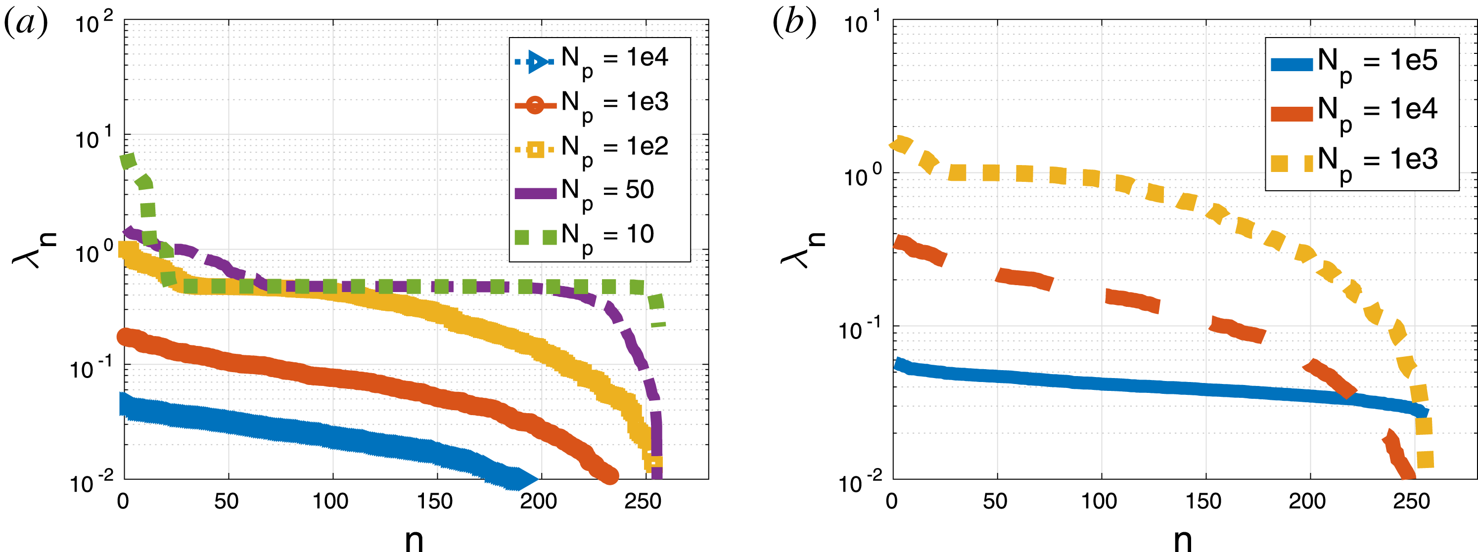
, see (4.3), plotted for different numbers of the ‘polarisation-density particles’. (a) Adiabatic electrons have been used. (b) The electrons are kinetic. One sees that the eigenvalues increase when the particle number goes down. The adiabatic-electron case (corresponding to the Helmholtz operator on the left-hand side of the quasi-neutrality equation) is more robust compared to the kinetic electrons (Laplace operator).

Note that (3.8) can be written as (see § 3 for the notations)
 $$\begin{eqnarray}\unicode[STIX]{x1D719}=(\bar{L}+{\hat{G}})^{-1}b+(\bar{L}+{\hat{G}})^{-1}({\hat{G}}-G)\unicode[STIX]{x1D719},\quad {\hat{G}}=(I+\hat{L}M^{-1})^{-1}L.\end{eqnarray}$$
The iterative solver described in this paper represents the classical Neumann series solution of this equation. Thus, one can gain insight into the convergence of the solver considering spectral properties of the operators
 $$\begin{eqnarray}N_{1}=(\bar{L}+{\hat{G}})^{-1}({\hat{G}}-G),\quad N_{2}=[\bar{L}+(\hat{L}M^{-1})\bar{L}+L]^{-1}[L-G-(\hat{L}M^{-1})G].\end{eqnarray}$$
These operators appear in (3.8) and (3.10). In our simulations, we use
 $N_{2}$
whereas
 $N_{1}$
is used in the derivation described in § 3. The spectral properties of
 $N_{1}$
and
 $N_{2}$
define if and how fast the Neumann series converge. In figure 5, the spectrum of
 $N_{2}$
is shown for different numbers of the numerical ‘polarisation-density particles’. On the left, the case of adiabatic-electron approximation (also used in figure 4) is shown. The kinetic electrons are shown on the right of figure 5. One sees that the maximal eigenvalue is much less than unity unless the particle resolution becomes too crude. This means that the convergence properties are good since the rate of the convergence in the direction of the
 $n$
th eigenvector is given by
 $|\unicode[STIX]{x1D706}_{n}|^{m}$
with
 $\unicode[STIX]{x1D706}_{n}$
being the corresponding eigenvalue and
 $m$
the iteration number. The convergence is good for all eigenvectors if all eigenvalues are smaller than unity. One can see that the simulations using adiabatic electrons are more robust compared to the kinetic-electron simulations: the largest eigenvalue
 $\max (|\unicode[STIX]{x1D706}_{n}|)$
is much smaller than unity for the adiabatic electrons at
 $N_{\text{p}}=1000$
whereas
 $\max (|\unicode[STIX]{x1D706}_{n}|)$
is larger than unity for the kinetic electrons at the same ‘polarisation-density particle’ resolution. For the adiabatic electrons, the value of
 $\max (|\unicode[STIX]{x1D706}_{n}|)$
approaches unity for
 $N_{\text{p}}=100$
. Note that in figure 4, the growth rate and the frequency are still quite accurate after only a single iteration despite the fact that
 $\max (|\unicode[STIX]{x1D706}_{n}|)\approx 0.8$
is not very small for
 $N_{\text{p}}=100$
. One can speculate that the direction along the eigenvector corresponding to the maximal eigenvalue is not very important for the solution. Only at
 $N_{\text{p}}=50$
with
 $\max (|\unicode[STIX]{x1D706}_{n}|)\approx 4$
the error in the frequency and the growth rate, shown in figure 4, becomes more pronounced. An effective reduction of the solution space as a consequence of the Fourier filtering (applied in the code) could also help removing the effect of undesired eigenvalues. One can numerically show that the spectra of
 $N_{1}$
and
 $N_{2}$
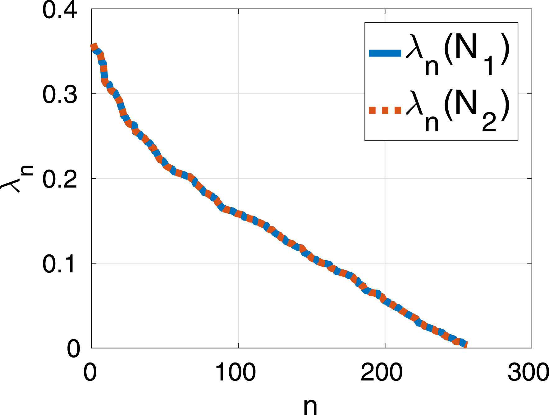
coincide, see figure 6. This provides an additional confirmation that the iterative scheme (3.16) is consistent.
The sorted eigenvalues (with the absolute values shown on the plot) of the operators
 $N_{1}$
and
 $N_{2}$
defined in (4.3) coincide, confirming the consistency of our solver. Here, the case corresponding to
 $N_{\text{p}}=10^{4}$
‘polarisation-density particles’ and adiabatic electrons is shown. Note the linear scale on the vertical axis of this plot (a logarithmic scale has been used in figure 5).

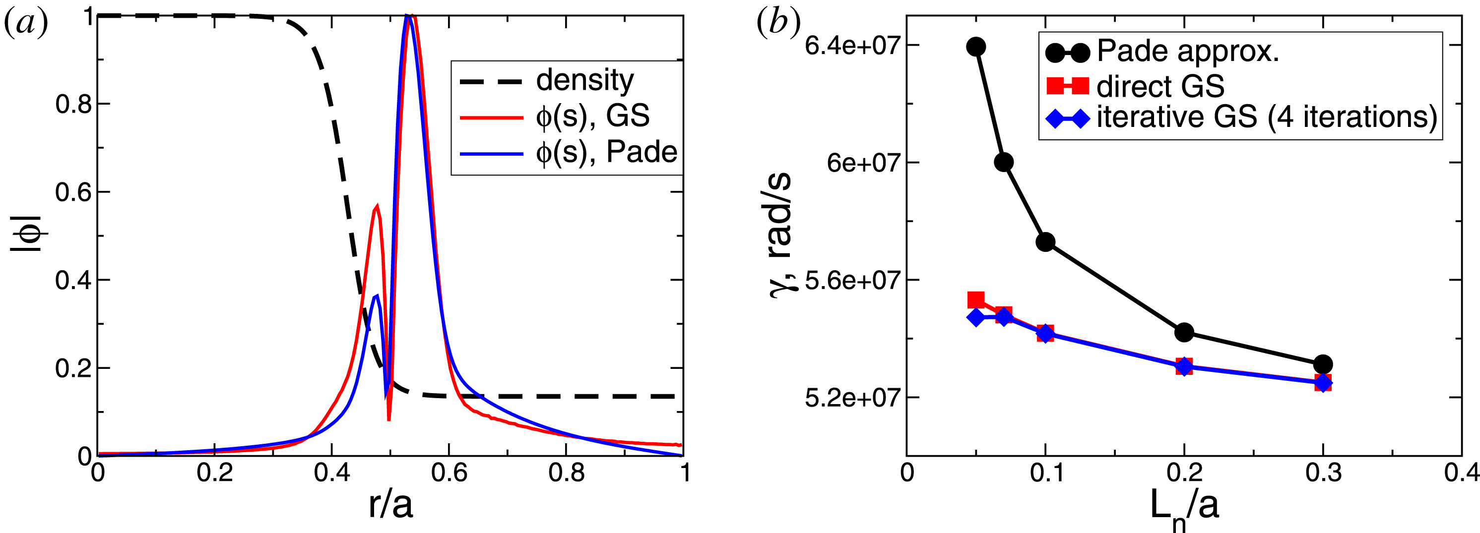
(a) Sheared-slab tearing mode (Zacharias, Kleiber & Hatzky Reference Zacharias, Kleiber and Hatzky2012) structure, computed using the generalised solver and the Padé approximation for the density profile shown and the density gradient length
 $L_{n}/a=0.05$
with
 $a$
the half-width of the simulation domain, see Zacharias et al. (Reference Zacharias, Kleiber and Hatzky2012) for details. (b) The growth rate of the sheared-slab tearing mode, destabilised by a parallel current, plotted as a function of the density gradient length for the density profile shown in (a). The direct generalised solver is compared to the iterative generalised solver and the Padé approximation. The motion of the ion gyro-centres has been suppressed.

In figure 7, the mode structure of the sheared-slab tearing mode (Zacharias et al. Reference Zacharias, Kleiber and Hatzky2012) is shown. The growth rate of the mode is plotted as a function of the density gradient length for the density profile shown in the figure. We compare the direct generalised solver, the iterative generalised solver with four iterations used here and the Padé approximation of the polarisation density. One sees that the agreement between the direct and iterative formulations of the generalised solver is good whereas the Padé approximation diverges from the correct result for large density gradients. The Padé-approximated growth rate can be much larger than the physical result for the parameters considered. This rather extreme numerical example demonstrates that our iterative scheme works even when the Padé approximation becomes poor. In such cases, more than one iteration is needed.
5 Nonlinear polarisation density
The weak formulation of the nonlinear quasi-neutrality condition, equation (1.1), with the phase-factor transformation equation (2.1) employed, is
 $$\begin{eqnarray}N_{\text{pol}}[\unicode[STIX]{x1D719}]=-\int \,\text{d}^{6}Z\frac{q_{\text{i}}^{2}}{B}\frac{\unicode[STIX]{x2202}f_{\text{i}}}{\unicode[STIX]{x2202}\unicode[STIX]{x1D707}}[\hat{\unicode[STIX]{x1D719}}-\unicode[STIX]{x1D6E5}_{\text{A}}\langle \hat{\unicode[STIX]{x1D719}}\unicode[STIX]{x1D6E5}_{\text{F}}\rangle ]\unicode[STIX]{x1D6EC}_{k}=b_{k}.\end{eqnarray}$$
Here,
 $f_{i}=f_{0\text{i}}+f_{1\text{i}}$
is the total nonlinear distribution function. The finite elements, the phase-factor transformed electrostatic potential, and the phase factors
 $\unicode[STIX]{x1D6E5}_{\text{(A,F)}}$
are computed at the position
 $\boldsymbol{R}+\unicode[STIX]{x1D746}$
. The charge assignment vector is
 $$\begin{eqnarray}b_{k}=\mathop{\sum }_{s=\text{i},\text{e}}q_{s}\int \,\text{d}^{6}Z\hat{f}_{1a}\unicode[STIX]{x1D6EC}_{k}\unicode[STIX]{x1D6E5}_{\text{A}}.\end{eqnarray}$$
After the integration by parts, one can write:
 $$\begin{eqnarray}N_{\text{pol}}[\unicode[STIX]{x1D719}]=\int \,\text{d}^{6}Z\frac{q_{\text{i}}^{2}}{B}f_{\text{i}}\frac{\unicode[STIX]{x2202}}{\unicode[STIX]{x2202}\unicode[STIX]{x1D707}}[\unicode[STIX]{x1D6EC}_{k}(\hat{\unicode[STIX]{x1D719}}-\unicode[STIX]{x1D6E5}_{\text{A}}\langle \hat{\unicode[STIX]{x1D719}}\unicode[STIX]{x1D6E5}_{\text{F}}\rangle )].\end{eqnarray}$$
Taking into account that for any
 $Q(\boldsymbol{R}+\unicode[STIX]{x1D746})$
 $$\begin{eqnarray}\frac{\unicode[STIX]{x2202}Q(\boldsymbol{R}+\unicode[STIX]{x1D746})}{\unicode[STIX]{x2202}\unicode[STIX]{x1D707}}=\frac{\unicode[STIX]{x2202}\unicode[STIX]{x1D746}}{\unicode[STIX]{x2202}\unicode[STIX]{x1D707}}\boldsymbol{\cdot }\unicode[STIX]{x1D735}Q=\frac{1}{2\unicode[STIX]{x1D707}}\unicode[STIX]{x1D746}\boldsymbol{\cdot }\unicode[STIX]{x1D735}Q,\quad \unicode[STIX]{x1D70C}=\sqrt{\frac{2\unicode[STIX]{x1D707}}{e\unicode[STIX]{x1D714}_{\text{c}}}}\end{eqnarray}$$
at a fixed
 $\boldsymbol{R}$
and using
 $\unicode[STIX]{x2202}\langle Q\rangle /\unicode[STIX]{x2202}\unicode[STIX]{x1D707}=\langle \unicode[STIX]{x2202}Q/\unicode[STIX]{x2202}\unicode[STIX]{x1D707}\rangle$
, we can write
 $$\begin{eqnarray}\displaystyle & \displaystyle \frac{\unicode[STIX]{x2202}}{\unicode[STIX]{x2202}\unicode[STIX]{x1D707}}(\hat{\unicode[STIX]{x1D719}}-\unicode[STIX]{x1D6E5}_{\text{A}}\langle \hat{\unicode[STIX]{x1D719}}\unicode[STIX]{x1D6E5}_{\text{F}}\rangle )=\frac{1}{2\unicode[STIX]{x1D707}} (\unicode[STIX]{x1D746}\boldsymbol{\cdot }\unicode[STIX]{x1D735}\hat{\unicode[STIX]{x1D719}}-\unicode[STIX]{x1D6E5}_{\text{A}}\langle \unicode[STIX]{x1D746}\boldsymbol{\cdot }\unicode[STIX]{x1D735}\hat{\unicode[STIX]{x1D719}}\unicode[STIX]{x1D6E5}_{\text{F}}\rangle + & \displaystyle\end{eqnarray}$$
 $$\begin{eqnarray}\displaystyle & \displaystyle +\,\text{i}\unicode[STIX]{x1D6E5}_{\text{A}}[\unicode[STIX]{x1D746}\boldsymbol{\cdot }\unicode[STIX]{x1D735}S\langle \hat{\unicode[STIX]{x1D719}}\unicode[STIX]{x1D6E5}_{\text{F}}\rangle -\langle \unicode[STIX]{x1D746}\boldsymbol{\cdot }\unicode[STIX]{x1D735}S\hat{\unicode[STIX]{x1D719}}\unicode[STIX]{x1D6E5}_{\text{F}}\rangle ]). & \displaystyle\end{eqnarray}$$
This leads to the nonlinear polarisation density in the matrix-free formulation:
 $$\begin{eqnarray}\displaystyle G\unicode[STIX]{x1D719}_{n} & = & \displaystyle \mathop{\sum }_{\unicode[STIX]{x1D708}=1}^{N_{\text{p}}}\frac{q_{\text{i}}^{2}}{2\unicode[STIX]{x1D707}_{\unicode[STIX]{x1D708}}B}(f_{0\unicode[STIX]{x1D708}}\unicode[STIX]{x1D701}_{\unicode[STIX]{x1D708}}+w_{\unicode[STIX]{x1D708}})\langle \!\unicode[STIX]{x1D6EC}_{k}(\unicode[STIX]{x1D746}\boldsymbol{\cdot }\unicode[STIX]{x1D735}\hat{\unicode[STIX]{x1D719}}_{n}-\unicode[STIX]{x1D6E5}_{\text{A}}\langle \unicode[STIX]{x1D746}\boldsymbol{\cdot }\unicode[STIX]{x1D735}\hat{\unicode[STIX]{x1D719}}_{n}\unicode[STIX]{x1D6E5}_{\text{F}}\rangle )\nonumber\\ \displaystyle & & \displaystyle +\,(\hat{\unicode[STIX]{x1D719}}_{n}\unicode[STIX]{x1D6E5}_{\text{F}}-\langle \hat{\unicode[STIX]{x1D719}}_{n}\unicode[STIX]{x1D6E5}_{\text{F}}\rangle )\unicode[STIX]{x1D6E5}_{\text{A}}\unicode[STIX]{x1D746}\boldsymbol{\cdot }\unicode[STIX]{x1D735}\unicode[STIX]{x1D6EC}_{k}+\text{i}\unicode[STIX]{x1D6EC}_{k}\unicode[STIX]{x1D6E5}_{\text{A}}(\unicode[STIX]{x1D746}\boldsymbol{\cdot }\unicode[STIX]{x1D735}S\langle \hat{\unicode[STIX]{x1D719}}_{n}\unicode[STIX]{x1D6E5}_{\text{F}}\rangle -\langle \unicode[STIX]{x1D746}\boldsymbol{\cdot }\unicode[STIX]{x1D735}S\hat{\unicode[STIX]{x1D719}}_{n}\unicode[STIX]{x1D6E5}_{\text{F}}\rangle )\!\rangle \!.\quad \nonumber\\ \displaystyle & & \displaystyle\end{eqnarray}$$
Here,
 $\unicode[STIX]{x1D746}\boldsymbol{\cdot }\unicode[STIX]{x1D735}S=m_{0}\unicode[STIX]{x1D746}\boldsymbol{\cdot }\unicode[STIX]{x1D735}\unicode[STIX]{x1D703}-n_{0}\unicode[STIX]{x1D746}\boldsymbol{\cdot }\unicode[STIX]{x1D735}\unicode[STIX]{x1D711}$
. Taking into account
 $\unicode[STIX]{x1D6E5}_{\text{A}}\unicode[STIX]{x1D6E5}_{\text{F}}=1$
, we can write
 $$\begin{eqnarray}\displaystyle G\unicode[STIX]{x1D719}_{n} & = & \displaystyle \mathop{\sum }_{\unicode[STIX]{x1D708}=1}^{N_{\text{p}}}\frac{q_{\text{i}}^{2}}{2\unicode[STIX]{x1D707}_{\unicode[STIX]{x1D708}}B}(f_{0\unicode[STIX]{x1D708}}\unicode[STIX]{x1D701}_{\unicode[STIX]{x1D708}}+w_{\unicode[STIX]{x1D708}})\langle \!\unicode[STIX]{x1D6EC}_{k}\unicode[STIX]{x1D6E5}_{\text{A}}(\unicode[STIX]{x1D6E5}_{\text{F}}\unicode[STIX]{x1D746}\boldsymbol{\cdot }\unicode[STIX]{x1D735}\hat{\unicode[STIX]{x1D719}}-\langle \unicode[STIX]{x1D6E5}_{\text{F}}\unicode[STIX]{x1D746}\boldsymbol{\cdot }\unicode[STIX]{x1D735}\hat{\unicode[STIX]{x1D719}}\rangle )\nonumber\\ \displaystyle & & \displaystyle +\,(\hat{\unicode[STIX]{x1D719}}\unicode[STIX]{x1D6E5}_{\text{F}}-\langle \hat{\unicode[STIX]{x1D719}}\unicode[STIX]{x1D6E5}_{\text{F}}\rangle )\unicode[STIX]{x1D6E5}_{\text{A}}\unicode[STIX]{x1D746}\boldsymbol{\cdot }\unicode[STIX]{x1D735}\unicode[STIX]{x1D6EC}_{k}\nonumber\\ \displaystyle & & \displaystyle +\,\text{i}\unicode[STIX]{x1D6EC}_{k}\unicode[STIX]{x1D6E5}_{\text{A}}(\unicode[STIX]{x1D746}\boldsymbol{\cdot }\unicode[STIX]{x1D735}S\hat{\unicode[STIX]{x1D719}}\unicode[STIX]{x1D6E5}_{\text{F}}-\langle \unicode[STIX]{x1D746}\boldsymbol{\cdot }\unicode[STIX]{x1D735}S\hat{\unicode[STIX]{x1D719}}\unicode[STIX]{x1D6E5}_{\text{F}}\rangle )-\text{i}\unicode[STIX]{x1D6EC}_{k}\unicode[STIX]{x1D6E5}_{\text{A}}\unicode[STIX]{x1D746}\boldsymbol{\cdot }\unicode[STIX]{x1D735}S(\hat{\unicode[STIX]{x1D719}}\unicode[STIX]{x1D6E5}_{\text{F}}-\langle \hat{\unicode[STIX]{x1D719}}\unicode[STIX]{x1D6E5}_{\text{F}}\rangle )\!\rangle \!.\qquad\end{eqnarray}$$
Here, the sum is taken over the same markers moving along the gyrokinetic orbits as those used for the charge assignment. The linear part of the polarisation density can also be computed using stationary ‘polarisation-density particles’ as described in § 4. A small number of these auxiliary ‘particles’ can be sufficient in this case in order to achieve a good accuracy, making the linear part of the solver computationally efficient. Another possibility is to compute the linear part of the polarisation density on the Eulerian grid as in Idomura (Reference Idomura2012) and Dominski et al. (Reference Dominski, McMillan, Brunner, Merlo, Tran and Villard2017) while using the Monte Carlo scheme only for the nonlinear part. Note that for the energy consistency, the equations of motion must be modified as in Idomura (Reference Idomura2012) and Mishchenko & Brizard (Reference Mishchenko and Brizard2011) when the nonlinear part of the polarisation density is included. In this paper, we limit our consideration to the basic formulation of the iterative numerical scheme which can also be used for more detailed studies of the nonlinear polarisation effect in future.
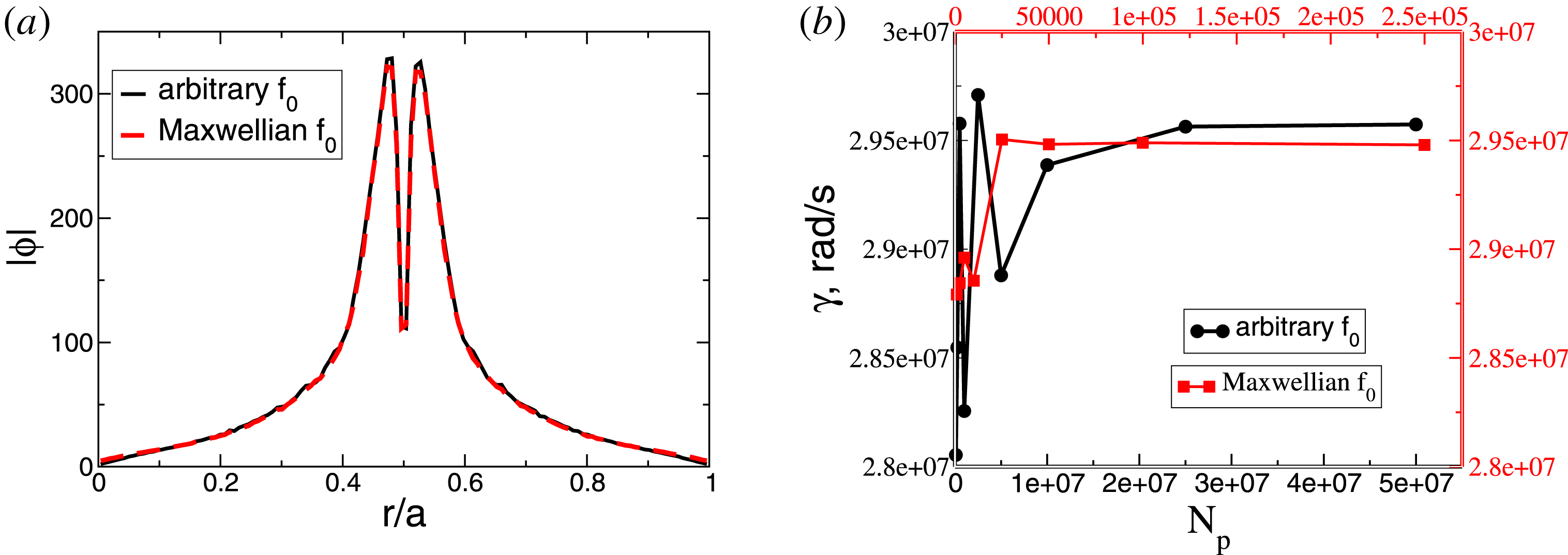
(a) The mode structure of the tearing instability computed using the linear part of the solver (5.8). The scheme based on (4.1) employing an analytically known Maxwellian distribution function is compared versus the scheme based on (5.8) which can be used for any, also nonlinear, distribution functions.
 $N_{\text{p}}=16\times 10^{6}$
is used for the arbitrary-distribution scheme.
 $N_{\text{p}}=10^{5}$
is used for the Maxwellian-distribution scheme. (b) The convergence with respect to the number of the polarisation-density particles. Note the different abscissa scales for the two schemes. The Maxwellian scheme, equation (4.1), converges more than two orders of magnitude faster since the importance sampling can be employed. One sees that the growth rates computed with the two schemes, equations (4.1) and (5.8) are in a good agreement with each other.

In figure 8, the mode structure of the tearing instability is shown computed using only the linear part of the solver (5.8), i.e. skipping
 $w_{\unicode[STIX]{x1D708}}$
on the right-hand side. This result is compared to the mode structure computed using the solver (4.1) which assumes that the distribution function is a Maxwellian. In contrast, the scheme based on (5.8) does not make this assumption and can therefore be used for any, even numerically determined, distribution function.
 $N_{\text{p}}=16\times 10^{6}$
is used for the arbitrary-distribution scheme.
 $N_{\text{p}}=10^{5}$
is used for the Maxwellian-distribution scheme. One sees that the agreement between the schemes in terms of the mode structure is very good.
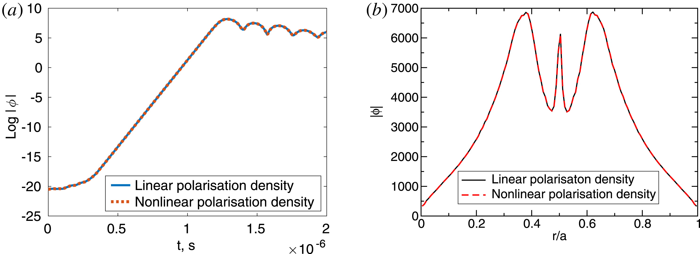
(a) The collisionless tearing mode (Zacharias et al.
Reference Zacharias, Kleiber and Hatzky2012) evolution in the nonlinear regime. The linear approximation of the polarisation density is compared with the nonlinear case. (b) The mode structure in the early nonlinear phase corresponding to
 $t=1.3\times 10^{-6}~\text{s}$
in (a). One sees that the effect of the polarisation-density nonlinearity is negligible for the case considered.

Figure 8(b), the convergence of the tearing mode growth rate is shown as a function of the number of the polarisation-density particles. Again, the scheme based on (4.1) is compared with the scheme based on (5.8). One sees that the Maxwellian-distribution scheme (4.1) converges much faster in terms of the number of the polarisation-density particles compared to the arbitrary-distribution scheme (5.8). This is a consequence of the importance sampling which can be employed in the first scheme to take into account the distribution function
 $f_{0\text{i}}$
, the gyrokinetic magnetic field
 $B$
, etc. One sees that the growth rate computed employing (5.8) is in a good agreement with the linear matrix-free solver based on (4.1). A small residual discrepancy between the growth rates can be attributed to other numerical parameters such as the number of the gyro-points. This result verifies the new solver which can be used also for the nonlinear polarisation density.
Finally, in figure 9, we plot the nonlinear evolution and the nonlinear mode structure of the tearing mode comparing simulations using linear and nonlinear polarisation densities. We use
 $N_{\text{e}}=32\times 10^{6}$
electron markers for the charge assignment in both simulations. The same markers are used to compute the nonlinear part of the polarisation density, equation (5.8). For the linear polarisation density, we use
 $N_{\text{p}}=5\times 10^{6}$
particles. One sees that the effect of the polarisation-density nonlinearity is negligible for the case of the tearing mode considered here. This may change for the edge plasma conditions, see (Yu et al.
Reference Yu, Krasheninnikov and Guzdar2006; Angus & Umansky Reference Angus and Umansky2014; Wiesenberger et al.
Reference Wiesenberger, Madsen and Kendl2014; Kendl Reference Kendl2015). Note that the other examples, such as the nonlinear shear Alfvén waves or nonlinear geodesic acoustic modes (GAMs), will require couplings between the different toroidal mode numbers (e.g. in order to drive the GAMs nonlinearly from the ITG turbulence), which is not available in the GYGLES code. These cases can be considered in future when the iterative nonlinear solver is implemented in a code, such as ORB5 (Jolliet et al.
Reference Jolliet, Bottino, Angelino, Hatzky, Tran, McMillan, Sauter, Appert, Idomura and Villard2007), which is more suited for the nonlinear simulations. Physically, the nonlinearity in the polarisation density is interesting since it can change the plasma inertia as a consequence of the perturbed motion of the ions. At short perpendicular scales, however, the perturbed ion motion is frequently suppressed as a consequence of the gyro-averaging. It seems, therefore, that the best way to physically relevant applications of the nonlinear polarisation density is considering long wavelengths, as usually appropriate for GAMs, with the perturbed ion response dominating. An additional advantage is that in this case a simpler scheme, based on the long-wavelength approximation, can be used, see appendix A.
6 Conclusions
An iterative formulation of the arbitrarily short-wavelength solver for global gyrokinetic simulations has been suggested. The solver has been verified against the solution of the dispersion relation. It can be used to treat the nonlinear polarisation density which can be important at the plasma edge. In the linear case, the solver has been shown to be computationally efficient since a moderate number of numerical particles and a single iteration are usually sufficient to provide a good accuracy. In future, this solver can be used to study multi-scale phenomena such as co-existing ITG and TEM instabilities. It is also of interest for global nonlinear gyrokinetic simulations of fusion plasmas including the plasma edge where both the strong density gradients and large-amplitude perturbations are present. In such a case, the usual approximations of the gyrokinetic polarisation density, the Padé approximation and the linear approximation, related to the gyro-fluid Boussinesq approximation (Yu et al. Reference Yu, Krasheninnikov and Guzdar2006; Angus & Umansky Reference Angus and Umansky2014; Wiesenberger et al. Reference Wiesenberger, Madsen and Kendl2014; Kendl Reference Kendl2015), can break down for the edge plasma conditions. In this paper, we have developed an approach overcoming these limitations.
Acknowledgements
We acknowledge P. Helander for his support. We thank S. Mochalskyy for his help with the eigenvalue ScaLAPACK solver. Numerical simulations were performed on the Marconi supercomputer within the framework of the EUGY project. This work has been carried out within the framework of the EUROfusion Consortium and has received funding from the Euratom research and training programme 2014–2018 and 2019–2020 under grant agreement no. 633053. The views and opinions expressed herein do not necessarily reflect those of the European Commission.
Appendix A
The long-wavelength approximation of the nonlinear quasi-neutrality equation in the adiabatic-electron approximation is
 $$\begin{eqnarray}\frac{q_{\text{e}}^{2}n_{0}}{T_{\text{e}}}(\unicode[STIX]{x1D719}-\bar{\unicode[STIX]{x1D719}})-\unicode[STIX]{x1D735}\boldsymbol{\cdot }\left(\frac{n_{\text{i}}}{B\unicode[STIX]{x1D714}_{\text{ci}}}\unicode[STIX]{x1D735}_{\bot }\unicode[STIX]{x1D719}\right)=q_{\text{i}}n_{1\text{i}},\end{eqnarray}$$
where
 $\bar{\unicode[STIX]{x1D719}}$
is the flux-surface average of the electrostatic potential,
 $n_{\text{i}}=n_{0}+n_{1\text{i}}$
,
 $n_{0}$
is the unperturbed density (assuming two species and quasi-neutrality) and
 $n_{1\text{i}}$
is the ion-density perturbation. This equation can be rewritten as
 $$\begin{eqnarray}\frac{q_{\text{e}}^{2}n_{0}}{T_{\text{e}}}(\unicode[STIX]{x1D719}-\bar{\unicode[STIX]{x1D719}})-\unicode[STIX]{x1D735}\boldsymbol{\cdot }\left(\frac{n_{0}}{B\unicode[STIX]{x1D714}_{\text{ci}}}\unicode[STIX]{x1D735}_{\bot }\unicode[STIX]{x1D719}\right)=q_{\text{i}}n_{1\text{i}}+\unicode[STIX]{x1D735}\boldsymbol{\cdot }\left(\frac{n_{1\text{i}}}{B\unicode[STIX]{x1D714}_{\text{ci}}}\unicode[STIX]{x1D735}_{\bot }\unicode[STIX]{x1D719}\right).\end{eqnarray}$$
Assuming that the perturbed ion density
 $n_{1\text{i}}$
is smaller than the unperturbed density
 $n_{0}$
(not necessarily much smaller), one can apply the Neumann series expansion resulting in
 $$\begin{eqnarray}\displaystyle & \displaystyle \frac{q_{\text{e}}^{2}n_{0}}{T_{\text{e}}}(\unicode[STIX]{x1D719}_{0}-\bar{\unicode[STIX]{x1D719}}_{0})-\unicode[STIX]{x1D735}\boldsymbol{\cdot }\left(\frac{n_{0}}{B\unicode[STIX]{x1D714}_{\text{ci}}}\unicode[STIX]{x1D735}_{\bot }\unicode[STIX]{x1D719}_{0}\right)=q_{\text{i}}n_{1\text{i}} & \displaystyle\end{eqnarray}$$
 $$\begin{eqnarray}\displaystyle & \displaystyle \frac{q_{\text{e}}^{2}n_{0}}{T_{\text{e}}}(\unicode[STIX]{x1D719}_{1}-\bar{\unicode[STIX]{x1D719}}_{1})-\unicode[STIX]{x1D735}\boldsymbol{\cdot }\left(\frac{n_{0}}{B\unicode[STIX]{x1D714}_{\text{ci}}}\unicode[STIX]{x1D735}_{\bot }\unicode[STIX]{x1D719}_{1}\right)=\unicode[STIX]{x1D735}\boldsymbol{\cdot }\left(\frac{n_{1\text{i}}}{B\unicode[STIX]{x1D714}_{\text{ci}}}\unicode[STIX]{x1D735}_{\bot }\unicode[STIX]{x1D719}_{0}\right). & \displaystyle\end{eqnarray}$$
Here, the electrostatic potential is expanded as
 $\unicode[STIX]{x1D719}=\unicode[STIX]{x1D719}_{0}+\unicode[STIX]{x1D716}\unicode[STIX]{x1D719}_{1}+\cdots \,$
with
 $\unicode[STIX]{x1D716}$
the Neumann expansion parameter. For convergence, we need
 $\unicode[STIX]{x1D716}<1$
. In the matrix form, we obtain
 $$\begin{eqnarray}\displaystyle (L+\bar{L})\unicode[STIX]{x1D719}_{0}=b,\quad (L+\bar{L})\unicode[STIX]{x1D719}_{m+1}=-L_{1}\unicode[STIX]{x1D719}_{m},m=0,1,\ldots & & \displaystyle\end{eqnarray}$$
 $$\begin{eqnarray}\displaystyle (L_{1}\unicode[STIX]{x1D719}_{m})_{k}=\int \frac{n_{1\text{i}}(\boldsymbol{x})}{B\unicode[STIX]{x1D714}_{\text{ci}}}\unicode[STIX]{x1D735}_{\bot }\unicode[STIX]{x1D719}_{m}(\boldsymbol{x})\boldsymbol{\cdot }\unicode[STIX]{x1D735}_{\bot }\unicode[STIX]{x1D6EC}_{k}(\boldsymbol{x})\,\text{d}^{3}x. & & \displaystyle\end{eqnarray}$$
The definitions of
 $L$
,
 $\bar{L}$
and
 $b$
can be found in § 3. The phase factor is dropped here since ORB5 (Jolliet et al.
Reference Jolliet, Bottino, Angelino, Hatzky, Tran, McMillan, Sauter, Appert, Idomura and Villard2007) does not have it. The spline coefficients for the perturbed density can be found from the charge-assignment vector
 $b$
using the mass matrix
 $M$
:
 $$\begin{eqnarray}q_{\text{i}}n_{1\text{i}}(\boldsymbol{x},t)=\mathop{\sum }_{k}n_{k}\unicode[STIX]{x1D6EC}_{k}(\boldsymbol{x}),\quad n_{k}=M_{kl}^{-1}b_{l},\quad b_{l}=q_{\text{i}}\mathop{\sum }_{\unicode[STIX]{x1D708}=1}^{N_{\text{p}}}w_{\unicode[STIX]{x1D708}}\langle \unicode[STIX]{x1D6EC}_{l}\rangle _{\unicode[STIX]{x1D708}}.\end{eqnarray}$$
A similar approach has been used by Angus & Umansky (Reference Angus and Umansky2014) in the fluid context.
The full gyrokinetic Hamiltonian including nonlinear terms (Brizard & Hahm Reference Brizard and Hahm2007) should be used in the equations of the gyro-centre motion when the polarisation density is nonlinear. Otherwise, the energy conservation is violated (Brizard Reference Brizard2010). In contrast, the nonlinear terms must be dropped in the gyrokinetic Hamiltonian when computing the gyro-centre orbits for the linearised polarisation density (Boussinesq approximation), see Brizard (Reference Brizard2010) for details. The need for more complicated gyro-centre orbits is, therefore, a direct consequence of the nonlinearity in the polarisation density (linked together by the variational principle and the energy conservation requirement).
In the electrostatic limit, the second-order Hamiltonian is
 $$\begin{eqnarray}\displaystyle & \displaystyle \bar{H}_{2}=-\frac{e^{2}}{2B}\frac{\unicode[STIX]{x2202}}{\unicode[STIX]{x2202}\unicode[STIX]{x1D707}}\langle \widetilde{\unicode[STIX]{x1D719}}^{2}\rangle =-\frac{e^{2}}{B}\left\langle \widetilde{\unicode[STIX]{x1D719}}\frac{\unicode[STIX]{x2202}\unicode[STIX]{x1D719}}{\unicode[STIX]{x2202}\unicode[STIX]{x1D707}}\right\rangle =-\frac{e^{2}}{2\unicode[STIX]{x1D707}B}\langle (\unicode[STIX]{x1D719}-\langle \unicode[STIX]{x1D719}\rangle )\unicode[STIX]{x1D746}\boldsymbol{\cdot }\unicode[STIX]{x1D735}\unicode[STIX]{x1D719}\rangle & \displaystyle\end{eqnarray}$$
 $$\begin{eqnarray}\displaystyle & \displaystyle \unicode[STIX]{x1D746}=\sqrt{\frac{2\unicode[STIX]{x1D707}}{e\unicode[STIX]{x1D714}_{\text{c}}}}\hat{\unicode[STIX]{x1D736}}=\frac{v_{\bot }}{\unicode[STIX]{x1D714}_{c}}\hat{\unicode[STIX]{x1D736}},\quad \hat{\unicode[STIX]{x1D736}}=-\boldsymbol{e}_{1}\cos \unicode[STIX]{x1D6FC}+\boldsymbol{e}_{2}\sin \unicode[STIX]{x1D6FC} & \displaystyle\end{eqnarray}$$
with
 $\unicode[STIX]{x1D6FC}$
the gyro-phase,
 $\widetilde{\unicode[STIX]{x1D719}}=\unicode[STIX]{x1D719}-\langle \unicode[STIX]{x1D719}\rangle$
,
 $\langle \unicode[STIX]{x1D719}\rangle$
the gyro-average and (5.4) has been used. The electrostatic gyro-centre orbits are given by the expressions (Brizard & Hahm Reference Brizard and Hahm2007):
 $$\begin{eqnarray}B_{\Vert }^{\star }\dot{\boldsymbol{R}}=\frac{1}{m}\frac{\unicode[STIX]{x2202}H}{\unicode[STIX]{x2202}v_{\Vert }}\boldsymbol{B}^{\star }-\frac{\unicode[STIX]{x1D735}H\times \boldsymbol{b}}{q},\quad B_{\Vert }^{\star }\dot{v}_{\Vert }=-\frac{\unicode[STIX]{x1D735}H\boldsymbol{\cdot }\boldsymbol{B}^{\star }}{m}.\end{eqnarray}$$
Here,
 $H=H_{0}+H_{1}+H_{2}$
is the gyrokinetic Hamiltonian, see Brizard & Hahm (Reference Brizard and Hahm2007) for notations and further details. Only the spatial derivative of
 $H_{2}$
, taken at a constant
 $\unicode[STIX]{x1D707}$
, is needed for the electrostatic approximation of the perturbed gyro-centre orbits:
 $$\begin{eqnarray}\unicode[STIX]{x1D735}H_{2}=-\frac{e^{2}}{2\unicode[STIX]{x1D707}}\unicode[STIX]{x1D735}\left[\frac{1}{B}\langle (\unicode[STIX]{x1D719}-\langle \unicode[STIX]{x1D719}\rangle )\unicode[STIX]{x1D746}\boldsymbol{\cdot }\unicode[STIX]{x1D735}\unicode[STIX]{x1D719}\rangle \right]\approx -\frac{m}{2}\unicode[STIX]{x1D735}\left(\frac{\unicode[STIX]{x1D735}_{\bot }\unicode[STIX]{x1D719}(\boldsymbol{R})}{B}\right)^{2}.\end{eqnarray}$$
Further elaboration and practical implementation of the long-wavelength non-Boussinesq scheme is a subject of future research.