2.1 Apparatus

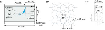
The main components of the experimental set-up consist of an open loop wind tunnel and a liquid injection system. The wind tunnel is designed to generate a uniform subsonic airflow in a transparent test section made of acrylic, which has a square cross-section of $305~\text{mm}\times 305~\text{mm}$ and a length of 600 mm (figure 1 a). The incoming airflow is made turbulent by placing at the inlet of the test section a perforated plate with a solidity ratio (i.e. solid area/total area) of $S=50\,\%$ (figure 1 b). The grid has a nominal mesh spacing of $M=16$  mm, a nominal hole diameter of $D=12$  mm and a thickness of $T=6$  mm. Two taper-edged nozzles with diameters of $d_{j}=1$ and 2 mm, and a fixed length to diameter ratio of $L/d_{j}=4$ , are used to inject the water jet ( $\unicode[STIX]{x1D707}_{l}=1.002\times 10^{-3}~\text{N}~\text{s}~\text{m}^{-2}$ , $\unicode[STIX]{x1D70C}_{l}=1001~\text{kg}~\text{m}^{-1}$ and $\unicode[STIX]{x1D70E}=0.072~\text{N}~\text{m}^{-1}$ ) transversely into the airflow in the test section. While there might be some degree of turbulence at the nozzle exit, which can influence the subsequent behaviour of the liquid jet breakup, this nozzle configuration was chosen to avoid the promotion of turbulence and cavitation of liquid flow inside the nozzle (Broumand & Birouk Reference Broumand and Birouk2017). The near-field characteristics of the liquid jet, such as mean velocity and turbulence intensity, for the nozzles used in this study are reported elsewhere (Broumand & Birouk Reference Broumand and Birouk2017). A schematic view of this nozzle is given in figure 1(c). As is illustrated in figure 1(a), the nozzle was centred transversely through the test section ceiling and inserted 24 mm into the cross-flow in order to avoid the effect of the wall boundary layer on liquid jet breakup, which causes a delay in its breakup time in comparison with that of a jet in a shock-tube facility (Osta & Sallam Reference Osta and Sallam2010). The nozzle exit was placed 200 mm downstream of the test section inlet (in the $x$ -axis direction) to avoid the turbulence developing region just downstream of the grid (Liu, Ting & Rankin Reference Liu, Ting and Rankin2004; Liu & Ting Reference Liu and Ting2007). The full characterization of the airflow in the wind tunnel’s test section is discussed later in § 2.3.

Figure 1.

Schematic diagram of (a) experimental set-up, (b) perforated plate pattern and (c) nozzle.

2.2 Diagnostics

Two-dimensional laser Doppler velocimetry (2D-LDV) measurements are performed along the centre plane of the wind tunnel’s test section at 23 spatial points, as indicated by the circles in figure 1(a) (positioned $x=12$ and $y=11$ apart), in order to capture the airflow characteristics, namely mean velocity and velocity fluctuations. The TSI LDV system consisted mainly of a 5 W coherent argon-ion laser, a fibre-light multicolour beam generator, a two-component fibre-optic transceiver for 514.5 and 488 nm, a photo detector module PDM 1000-12 and multibit digital burst correlator FSA 4010. A minimum of 20 000 LDV data samples were collected for each airflow speed to ensure reasonable statistical averaging of the axial mean velocity and its fluctuating turbulent component. Particle image velocimetry (PIV) was also used to estimate the integral length scale. The PIV set-up consisted of a Nd:YAG laser with a maximum pulse energy of 135 mJ at a repetition rate of 10 Hz, a double-frame FlowSense EO 4M CCD camera of 20.4 f.p.s. with a $2048\times 2048~\text{pixel}^{2}$ resolution and a Dantec Dynamic Studio Software. The duration between PIV laser pulses was adjusted between 40 and $60~\unicode[STIX]{x03BC}\text{s}$ depending on the selected cross-flow velocity. Three thousand image pairs were acquired using a field of view of $160\times 160~\text{mm}^{2}$ , as indicated by the dashed box in figure 1(a). Postprocessing of PIV images was performed using an interrogation area of $32\times 32$ with 50 % overlap along with a range validation to eliminate spurious vectors. In addition, an average filter of $3\times 3$ vectors was used for flow field smoothing. For both LDV and PIV, olive oil drops of approximately $1~\unicode[STIX]{x03BC}\text{m}$ were used as seeding particles of the gaseous cross-flow. The uncertainty of the measured airflow mean velocity with the LDV was estimated within $\pm 0.4~\text{m}~\text{s}^{-1}$ , and the uncertainty associated with the PIV measurements was within $\pm 1\,\%$ .

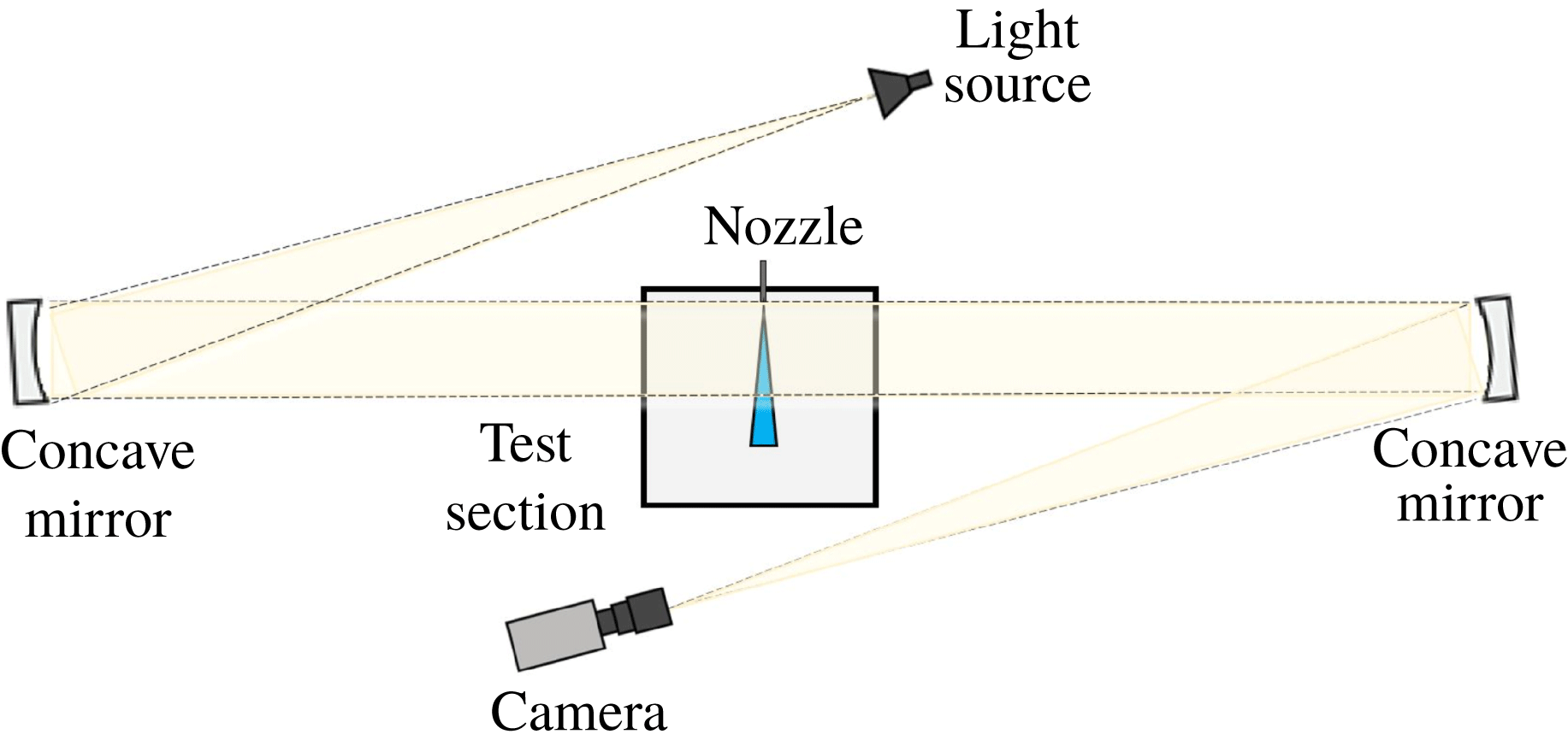
Shadowgraph technique was used to image the liquid jet and determine its trajectory and column breakup location. The adopted Z-type set-up consisted of a CMOS high-speed camera with a frame rate of 1040 fps at a resolution of $1280\times 1024~\text{pixel}^{2}$ , a pair of spherical parabolic concave mirrors with a diameter of 152.4 mm and a focal length of 1143 mm and a light source (figure 2). The camera was placed on the focal point of the second mirror where the reflected light from the second mirror was focused. For each test condition, 815 images were collected using an exposure time of $15~\unicode[STIX]{x03BC}\text{s}$ , which was found suitable to freeze droplets (with no blurring) at each frame with a satisfactory background brightness level. An in-house developed MATLAB code was used to estimate the jet trajectory and column breakup location.

Figure 2.

Schematic diagram of the imaging system.

2.3 Airflow characteristics and test conditions

The airflow local fluctuating velocity root-mean-square (r.m.s.) is altered at constant mean flow velocity using a turbulence-generating grid. Varying velocity fluctuations allows for a systematic examination of the effect of airflow turbulence on the breakup of a transverse liquid jet (Kourmatzis & Masri Reference Kourmatzis and Masri2015). The power-law decay region downstream of a grid in a wind tunnel is often used as an experimental benchmark for the evaluation of turbulence theories as it provides an empirical approximation of homogeneous, isotropic turbulence which can be produced easily in a laboratory set-up (Mohamed & Larue Reference Mohamed and Larue1990; Krogstad & Davidson Reference Krogstad and Davidson2010; Isaza, Salazar & Warhaft Reference Isaza, Salazar and Warhaft2014). LDV and PIV measurements were used to characterize the cross-airflow in the absence of a liquid jet but with the nozzle mounted in the test section.

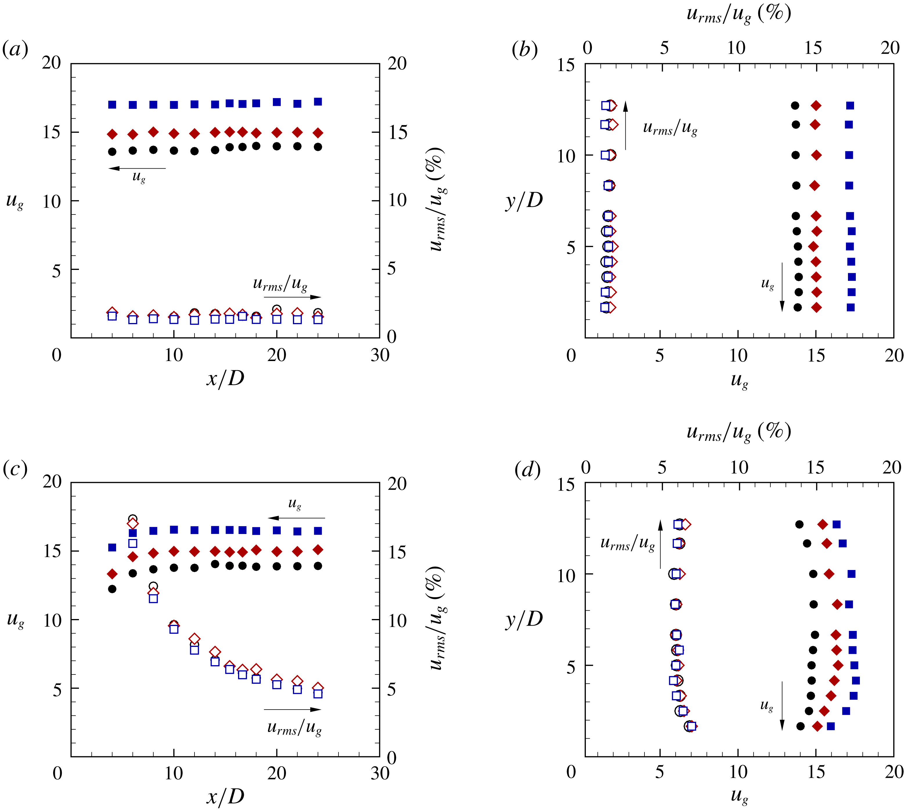
Figure 3 illustrates the LDV dataset for different cross-airflow streamwise mean velocity, $u_{g}=13.6$ , 15 and $17~\text{m}~\text{s}^{-1}$ . These velocities are kept similar for both no-grid and grid test conditions, while the r.m.s. of their corresponding streamwise mean velocity fluctuation $u_{rms}$ , normalized by $u_{g}$ , is varied. These plots are for the region confined within the test section (figure 1 a), where the horizontal direction is along the centreline of the test section at $y=152.5$  mm from right to left, and the vertical direction is at the nozzle location, $x=200$  mm, downwards from the nozzle-exit region to the centreline, as shown in figure 1(a). Figures 3(a) and 3(b) confirmed that, for the no-grid test condition, $u_{g}$ and its corresponding $u_{rms}$ are constant throughout the test section in the $x$ and $y$ directions, respectively. For the grid test condition, nonetheless, $u_{rms}$ experiences a gradual drop in the $x$ direction, while $u_{g}$ is unchanged (figure 3 c).This is due to the fact that the airflow is in the turbulence power-law decay region (Liu et al. Reference Liu, Ting and Rankin2004; Liu & Ting Reference Liu and Ting2007). The injection of the liquid at $x=200$  mm is, therefore, chosen in order to have a nearly constant turbulence intensity in the horizontal direction throughout the imaging field of view. Figure 3(d) shows that $u_{g}$ and $u_{rms}$ are almost unchanged in the vertical direction at the liquid injection point, with a very small deviation at small $y/D\approx 2{-}4$ due to the acceleration of airflow above the nozzle. Overall, as depicted in figure 3, it is clear that the airflow mean velocity does not have an influence on the cross-airflow turbulence intensity; however, using the turbulence-generating grid increases the normalized $u_{rms}$ from approximately $u_{rms}/u_{g}=1.5\,\%$ , for no grid, to $u_{rms}/u_{g}=5.5\,\%$ for the grid test conditions.

Figure 3.

Cross-flow streamwise mean velocity, $u_{g}$ (filled symbols), and normalized velocity r.m.s. $u_{rms}/u_{g}$ (open symbols) for the no-grid test in the (a)  $x$ -direction, (b)  $y$ -direction, and the grid test in the (c)  $x$ -direction, (d)  $y$ -direction; for three different mean velocities: $u_{g}=13.6$ (● and ○), 15 (♦ and ♢) and $17~\text{m}~\text{s}^{-1}$ (▪ and ▫). The distance axes are normalized by the grid orifice diameter $D$ .

The integral length scale, $L$ , of the cross-airflow at the nozzle exit was obtained experimentally using PIV. The turbulent Reynolds number, $Re_{L}=u_{rms}L/\unicode[STIX]{x1D708}$ , was then calculated based on $u_{rms}$ and $L$ for each test condition, where $\unicode[STIX]{x1D708}$ is the kinematic viscosity of air at room temperature and pressure test conditions (i.e. 298 K and 100 kPa). The turbulence integral time scale of the airflow, $\unicode[STIX]{x1D70F}$ , was estimated as $L/u_{g}$ based on Taylor’s frozen turbulence hypothesis, as $u_{rms}$ is less than 10 % of $u_{g}$ (Liu et al. 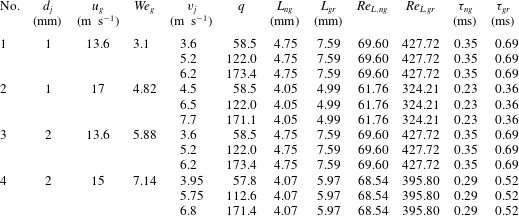Reference Liu, Ting and Rankin2004; Liu & Ting Reference Liu and Ting2007). Table 1, lists the test conditions of the present study.

Table 1.

Experimental test conditions and airflow turbulence characteristics.

According to table 1, for each value of $u_{g}$ , the turbulent integral length scale, and its corresponding time scale, as well as turbulent Reynolds numbers all depend on the grid. In addition, the values of these parameters decrease with increasing $u_{g}$ for both no-grid and grid test conditions.

3.1 Liquid jet primary breakup regime

Shadowgraph images of the test cases in table 1 were compared for both no-grid and grid test conditions in order to investigate the effect of velocity fluctuations of the cross-airflow on the primary breakup mechanism of a liquid jet. In agreement with the literature, it is observed that the breakup mode of the liquid jet injected into the cross-flow for both no-grid and grid test conditions changes from enhanced capillary breakup to the bag breakup regime when increasing $We_{g}$ from 3.1 to 7.14. At low $We_{g}=3.1$ (case No. 1), the liquid jet is curved by aerodynamics forces which are not large compared to surface tension forces. Nonetheless, aerodynamic forces accelerate the breakup processes caused by capillary forces. Hence, this regime is referred to as enhanced capillary breakup (Wu et al. Reference Wu, Kirkendall, Fuller and Nejad1997; Sallam et al. Reference Sallam, Aalburg and Faeth2004) (see movie 1 in the supplementary material available at https://doi.org/10.1017/jfm.2019.704 for case No. 1). Increasing further the cross-airflow velocity (cases No. 3 and 4) causes aerodynamic forces to dominate the breakup process. Bag-like structures are formed along the liquid column which exhibits breakup behaviour similar to that of the secondary breakup of a spherical droplet. This regime is referred to as bag breakup (Wu et al. Reference Wu, Kirkendall, Fuller and Nejad1997; Sallam et al. Reference Sallam, Aalburg and Faeth2004) (see movie 2 in the supplementary material for case No. 4). In both cases; i.e. no-grid and grid test conditions, while the breakup regimes for cases No. 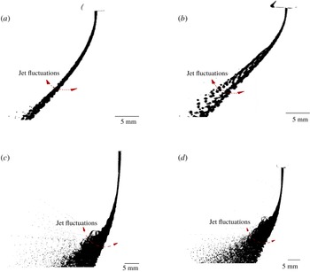1, 3 and 4 exhibit similar trends with increasing $We_{g}$ , it is observed that the higher velocity fluctuations of the grid test condition causes the liquid jet to fluctuate (i.e. displace normal to its axis) in the airflow more than no-grid test condition. This phenomenon can be seen in figure 4 for cases No. 1 and No. 4 by superimposing 10 successive liquid jet images at each test conditions. The same can be observed in movies 1 and 2 in the supplementary material.

Figure 4.

Superposition of 10 successive images of a liquid jet injected from a $d_{j}=1$  mm nozzle at $v_{j}=3.6~\text{m}~\text{s}^{-1}$ and $u_{g}=13.6~\text{m}~\text{s}^{-1}$ (case No. 1) with (a) no grid and (b) grid, and injected from a $d_{j}=2$ nozzle at $v_{j}=3.95~\text{m}~\text{s}^{-1}$ and $u_{g}=15~\text{m}~\text{s}^{-1}$ (case No. 4) with (c) no grid and (d) grid.

It is also observed that, in case No. 2, the presence of higher airflow velocity fluctuations at the grid test condition compared to the no-grid case causes the transition in the breakup regime to occur with a delay in the former case. In other words, while the liquid jet in case No. 1 (see table 1) breaks up in the enhanced capillary breakup regime, for both no-grid and grid test conditions. 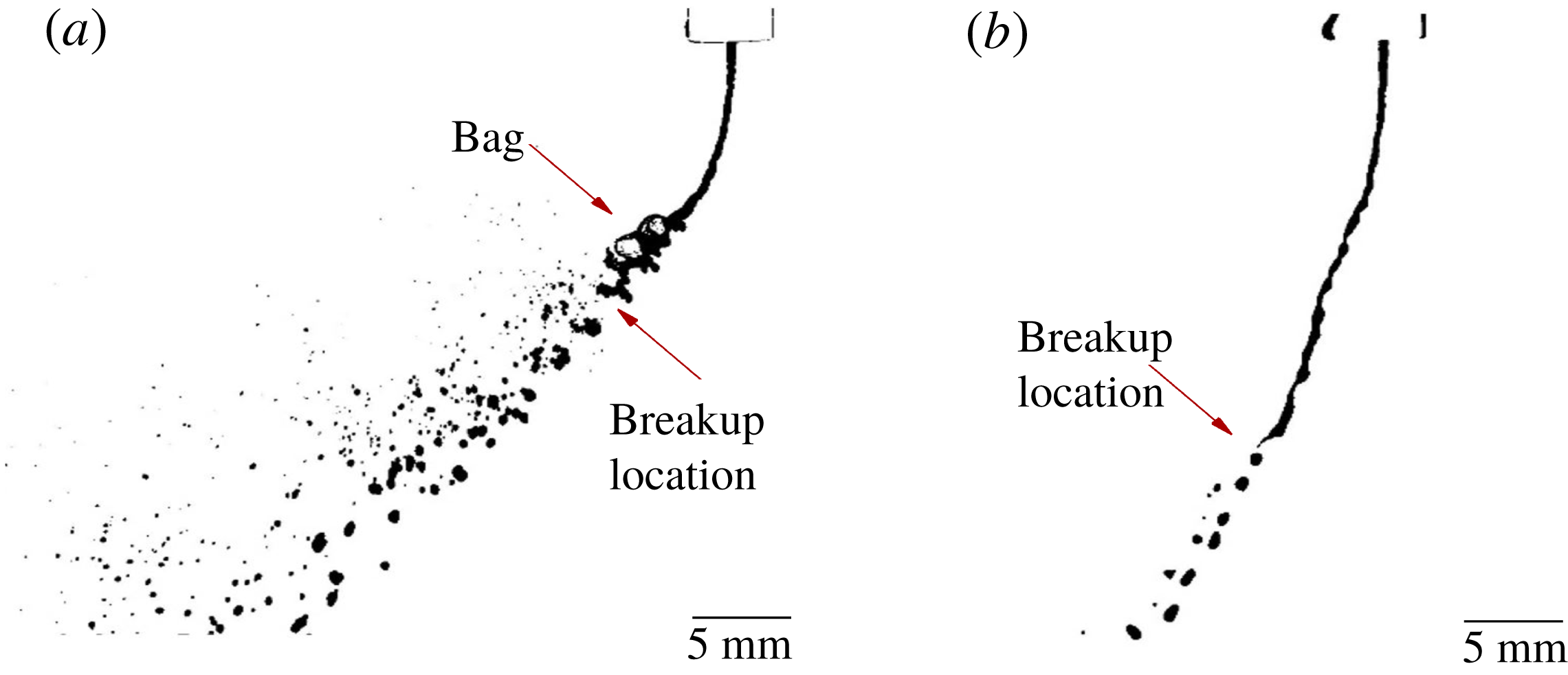By increasing $We_{g}$ according to the conditions of case No. 2, it is observed that the liquid column tends to break up in the capillary mode rather than in the bag breakup mode for the grid test conditions (see figure 5, and movie 3 in the supplementary material). Nonetheless, increasing further the airflow velocity, according to cases No. 3 and 4 (table 1), causes bag-like structures to form along the liquid column in both cases; i.e. no-grid and grid test conditions.

Figure 5.

Visualization of a liquid jet injected from a $d_{j}=1$  mm nozzle at $v_{j}=4.5~\text{m}~\text{s}^{-1}$ and $u_{g}=17~\text{m}~\text{s}^{-1}$ (case No. 2) with (a) no grid and (b) grid.

Similar late transitional behaviour of the jet breakup mechanism in a turbulent cross-airflow for ethyl-alcohol as the working liquid was observed in our recent study (Broumand, Ahmed & Birouk Reference Broumand, Ahmed and Birouk2019). This peculiar behaviour could be due to the higher fluctuations of the liquid jet in the cross-airflow in the presence of a grid (grid condition), which thus prevents the formation of a stable liquid sheet/membrane perpendicular to the airflow for bag formation. To gain an insight into this phenomenon, liquid jet dynamics is investigated in the following subsection.

3.2 Liquid jet dynamics

Proper orthogonal decomposition (POD) was applied to the series of shadowgraph images to identify the coherent structures/waves that appear along the surface of the liquid jet. POD is an optimal method for describing multidimensional datasets with a reduced number of dimensions (Pearson Reference Pearson1901). In the context of fluid mechanics, while the use of POD is well established to analyse velocity (i.e. vector) fields to identify the dominant modes or coherent structures in a flow field (Nobach et al. Reference Nobach, Tropea, Cordier, Bonnet, Delville, Lewalle, Farge, Schneider and Adrian2007; Holmes et al. Reference Holmes, Lumley, Berkooz and Rowley2012), it has been recently applied to a scalar field (i.e. pixel intensity/illumination of images) to study the features of a liquid jet or sheet. Arienti & Soteriou (Reference Arienti and Soteriou2009) applied this method to compare the wave structure of turbulent and non-turbulent transverse liquid jets. Later on, Herrmann et al. (Reference Herrmann, Arienti and Soteriou2011) used the same approach in their numerical results to study the effect of air/liquid density ratio on the surface waves of a transverse liquid jet. Similar approach is also employed by Prakash et al. (Reference Prakash, Sinha, Tomar and Ravikrishna2018) to study the effect of the liquid entry conditions on the structure of a transverse liquid jet. In other studies, Charalampous & Hardalupas (Reference Charalampous and Hardalupas2014) and Rajamanickam & Basu (Reference Rajamanickam and Basu2017) employed POD to investigate surface instabilities of co-axial liquid jets, and a liquid sheet in a co-annular swirl airflow, respectively.

Regarding liquid jet dynamics in a cross-airflow, POD can decouple the large flow features from small ones in a way such that the first intense modes represent the bulk column fluctuation while the following modes are attributed to the travelling waves (Arienti & Soteriou Reference Arienti and Soteriou2009). It is known that a travelling wave is a superposition of two standing waves (i.e. two conjugate modes) with half a wavelength delay, the same frequency and a phase difference of $\pm 90^{\circ }$ (Arienti & Soteriou Reference Arienti and Soteriou2009; Herrmann et al. Reference Herrmann, Arienti and Soteriou2011). The wavelength of the associated coherent structures can then be extracted directly by finding the distance between consecutive positive or negative peaks in these two modes. In the present study, therefore, the same approach was applied to a dataset of $N=815$ shadowgraph images with a POD field of view of $m\times n=100\times 400~\text{pixel}^{2}$ to estimate the upwind wavelength of the liquid jet at each test condition. The POD field of view was chosen to be near the nozzle region in order to identify the onset of dominant features on the liquid jet surface as their wavelengths become progressively stretched as the liquid jet penetrates into the cross-airflow (Arienti & Soteriou Reference Arienti and Soteriou2009; Li & Soteriou Reference Li and Soteriou2016). Using an in-house developed MATLAB code, the raw images were first subtracted from the background image (i.e. without droplets), and then the information in each pixel was translated into its intensity/illumination over a range from 0 to 255. After that, the so-called snapshot POD proposed by Sirovich (Reference Sirovich1987) was used for the orthogonal decomposition of the information. A detailed description of the algorithm and some relevant concepts are documented in Meyer, Pedersen & Özcan (Reference Meyer, Pedersen and Özcan2007), which is essentially a singular value decomposition technique (Chatterjee Reference Chatterjee2000). As a result, the orthonormal basis functions $\unicode[STIX]{x1D719}_{r}$ and time-dependent orthonormal amplitude coefficients (temporal coefficients) $a_{r,i}$ are extracted in a way that a reconstructed image with the first $M\leqslant N$ modes at time $t_{i}$ , $i=1,2,\ldots ,N$ , using (3.1), is optimal by minimizing the least squares truncation error. Finally, to identify the two conjugate modes, power spectrum density (PSD) of the series of temporal coefficients in the frequency domain was extracted (Nobach et al. Reference Nobach, Tropea, Cordier, Bonnet, Delville, Lewalle, Farge, Schneider and Adrian2007).

(3.1) $$\begin{eqnarray}Z_{i}=\mathop{\sum }_{r=0}^{M}a_{r,i}\unicode[STIX]{x1D719}_{r}.\end{eqnarray}$$

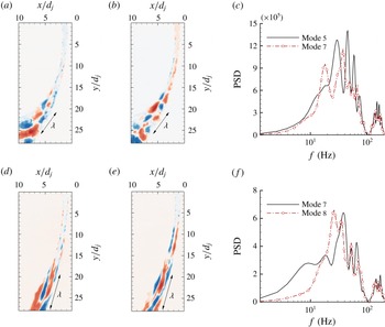
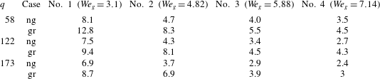
Applying the above-mentioned approach to, for example, case No. 2 with $q=58$ results in a non-dimensional wavelength of $\unicode[STIX]{x1D706}/d_{j}=4.7$ for the no-grid condition, and of $\unicode[STIX]{x1D706}/d_{j}=8.3$ for the grid condition. This clearly shows the elongation of the wave structures on the liquid jet surface due to higher velocity fluctuations of the turbulent cross-airflow. At this transitional condition, therefore, it can be concluded that the presence of longer wavelength axial instabilities on the jet’s surface (compared to the no-grid condition) along with surface tension forces cause the liquid column to break up in the capillary mode rather than in the bag breakup mode, where the aerodynamic drag forces of the cross-airflow are more effective. Figure 6 shows the two orthogonal modes with similar patterns and their corresponding PSD for both no-grid and grid conditions in case No. 2 with $q=58$ .

Figure 6.

Proper orthogonal decomposition and power spectrum density in case No. 2 with $v_{j}=4.5~\text{m}~\text{s}^{-1}$ for no-grid condition (a) POD mode 5, (b) POD mode 7 and (c) PSD of modes 5 and 7; and grid condition (d) POD mode 7, (e) POD mode 8 and (f) PSD of modes 7 and 8.

Table 2.

Non-dimensional wavelength $\unicode[STIX]{x1D706}/d_{j}$ of the liquid jet at different $We_{g}$ .

Similar growth in $\unicode[STIX]{x1D706}/d_{j}$ as a result of the turbulent nature of the cross-airflow was observed for the other cases (see table 2), but their breakup regimes were not altered as they are far from the transition borderline. Nonetheless, consistent with the literature (Mazallon et al. Reference Mazallon, Dai and Faeth1999; Sallam et al. Reference Sallam, Aalburg and Faeth2004; Amini Reference Amini2018), the non-dimensional surface wavelength decreased with increasing $We_{g}$ , or in other words, it decreased when the liquid jet breakup regime changes from capillary to bag breakup mode, in the case of both the no-grid and grid test conditions. The jet’s wavelength also slightly decreases with increasing $q$ at each specific $We_{g}$ at both, no-grid and grid, test conditions, but its effect on the jet’s wavelength is not as large as when increasing $We_{g}$ .

An extensive research effort has been devoted in the literature towards understanding the underlying physics of the origin of such instability waves in a transverse liquid jet by exploiting hydrodynamic instability analysis (Mazallon et al. Reference Mazallon, Dai and Faeth1999; Sallam et al. Reference Sallam, Aalburg and Faeth2004; Behzad et al. Reference Behzad, Ashgriz and Mashayek2015; Li & Soteriou Reference Li and Soteriou2016; Amini Reference Amini2018). It is known that small disturbances on the surface of a liquid jet in the presence of a uniform cross-airflow cause an unbalance between the pressure gradient and density gradient, leading to the RT instability in the region farther away from the nozzle exit (Li & Soteriou Reference Li and Soteriou2016; Li et al. Reference Li, Gao and Soteriou2017; Li & Soteriou Reference Li and Soteriou2018). In addition, the KH instability is a result of the presence of a tangential velocity gradient at the liquid/gas interface, which can amplify any disturbances on the jet surface, including the initial perturbations generated at the nozzle exit (Li & Soteriou Reference Li and Soteriou2016; Li et al. Reference Li, Gao and Soteriou2017; Li & Soteriou Reference Li and Soteriou2018). As such, increasing both the airflow velocity (which yields an increase in $We_{g}$ ) and liquid jet velocity (which increases $q$ ) results in shorter wavelength disturbances due to the amplification of RT and KH instabilities, respectively. Nonetheless, the effect of the latter is much smaller than the former due to the suppressed liquid flow turbulence at the nozzle exit and the high liquid/gas density ratio. Similarly, the elongation of the wave structures on the liquid jet surface when injected into a turbulent cross-airflow can be explained using hydrodynamic instability. This is due to the fact that the higher fluctuations of the liquid jet in a turbulent cross-airflow disturb the formation of the pressure gradient normal to the liquid/gas interface, which is the origin of the RT instability, and consequently weaken the RT instability mechanism.

Comparing the relationship between two length scales (namely, airflow integral length scale and jet surface wavelength) can also explain why the liquid jet in the enhanced capillary breakup mode is more stretched in a turbulent cross-airflow than under the bag breakup regime. In fact, it can be stated that, with increasing $We_{g}$ , as the jet surface wavelength (table 2) approaches the airflow integral length scale or becomes smaller (table 1), the influence of turbulent cross-airflow (i.e. grid condition) on the liquid jet instabilities is reduced. Overall, with the exception of the transition borderline between these two regimes (case No. 2), it is expected that the higher velocity fluctuations of the airflow further destabilize the liquid jet, and thus lead to the enhancement of its primary breakup (i.e. shorter breakup height and more bending into the cross-airflow) at each specific breakup regime, namely the enhanced capillary breakup regime (case No. 1) and bag breakup regime (cases No. 3 and 4). This qualitative observation will be quantified in the next sections by studying the liquid jet’s trajectory and its breakup height under different test conditions.

3.3 Liquid jet trajectory

In order to examine the effect of the presence of velocity fluctuations in cross-airflow on the mean liquid jet trajectory, measurements in the spray region were carried out employing the shadowgraph imaging method. In doing so, for each test condition in table 1, the background image (i.e. without liquid jet) was subtracted from the raw images, then the individual images were converted to binary images using a certain threshold and finally averaged to identify the windward boundary of the liquid jet. A threshold of 19 % of the highest pixel value of the 8-bit grey scale image was selected for all 815 images of each case such that it can successfully distinguish between droplet boundaries and their surroundings. The experimental uncertainties in the measurements of liquid jet trajectory were estimated to be $\pm 5\,\%$ . 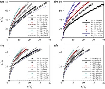Figures 7(a) to 7(d) depict the windward trajectories of the liquid jet injected into the cross-airflow at all $We_{g}$ values in table 1, which correspond to the enhanced capillary breakup and bag breakup for both no-grid and grid test conditions. As was expected for all breakup regimes, the liquid jet penetrates farther into the cross-airflow when increasing $q$ . More importantly, for both breakup regimes at a fixed value of $q$ and $We_{g}$ , using a grid causes the liquid jet to bend earlier into the airflow. This phenomenon is an indication of the pronounced effect of the cross-airflow turbulence on the trajectory of the liquid jet. It should be noted that, in case No. 2 (figure 7 b), the use of a grid has a noticeable effect on the liquid jet trajectory as the basic mechanism of the liquid jet breakup is altered. In this case, the liquid jet injected into the airflow at the grid test condition (i.e. turbulent conditions) breaks up in the enhanced capillary regime and exhibits a greater penetration compared to that in the bag breakup regime under the no-grid test condition (i.e. no turbulence).

Figure 7.

Effect of turbulent cross-airflow on the liquid jet’s trajectory with different velocities for (a) case No. 1, (b) case No. 2, (c) case No. 3 and (d) case No. 4.

To quantify the effect of the airflow turbulence properties, an empirical correlation is proposed for predicting the liquid jet trajectory which includes the turbulent Reynolds number, $Re_{L}=u_{rms}L/\unicode[STIX]{x1D708}$ . Following the analytical trajectory correlation proposed by Wu et al. (Reference Wu, Kirkendall, Fuller and Nejad1997) ( $y/d_{j}=C\sqrt{(x/d_{j})q}$ , where $C$ is a constant), $q$ was taken into account as the predominant parameter for predicting the windward trajectory of a liquid jet. Nonetheless, correlating the jet trajectory merely with $q$ was found to be inadequate to capture the effect of the contribution of the airflow’s turbulence to the liquid jet trajectory. Therefore, in addition to $q$ , we propose to correlate the liquid jet trajectory with $Re_{L}$ , in order to account for the cross-airflow turbulence. A nonlinear regression analysis was performed to determine the best fit of the jet trajectory experimental data within the range of all parameters examined in the present study, as given in table 1, which resulted in the following power-law correlation:

(3.2) $$\begin{eqnarray}y/d_{j}=C[(x/d_{j})q]^{0.5}Re_{L}^{-0.07},\end{eqnarray}$$

where $C$ depends mainly on the nozzle’s discharge coefficient ( $C_{d}$ ); i.e. $C\cong 2.3$ for $v_{j}\leqslant 4~(\text{m}~\text{s}^{-1})$ , and $C\cong 2.0$ for $4\leqslant v_{j}\leqslant 8~(\text{m}~\text{s}^{-1})$ . In the present study, in order to calculate $q$ , $v_{j}$ was estimated based on the volumetric flow rate divided by the liquid injector cross-sectional area. Nonetheless, the actual jet velocity at the nozzle exit, which depends on the nozzle’s orifice geometry, can be estimated as $v_{j}/C_{d}$ , where $C_{d}$ is the nozzle’s discharge coefficient (Brown, Mondragon & McDonell Reference Brown, Mondragon and McDonell2007); where $C$ in (3.2) was found inversely proportional to $C_{d}$ . The reduction of $C$ with increasing $v_{j}$ is consistent with the change in $C_{d}$ of the present nozzle, whose information is reported in our previous study (Broumand & Birouk Reference Broumand and Birouk2017), where the value of $C_{d}$ gradually increases from approximately ${\approx}$ 0.65–0.7 to approximately ${\approx}$ 0.8–0.85 with increasing liquid jet velocity in the range of $q<100$ , and remains constant in the high velocity (or $q$ ) range. The correlation coefficient of the regression analysis for the overall test conditions was 0.99, and the standard error of the fit was 0.05. A comparison between the experimental and prediction (proposed (3.2)) of the liquid jet trajectory for all the cases is shown in figure 7. It is clear that including the airflow turbulent Reynolds number with a negative power in the trajectory correlation to reflect the effect of the airflow’s turbulence properties provides realistic predictions over the range of parameters examined in the present paper (the only exception concerns the transition borderline at grid test condition (case No. 2)).

3.4 Liquid jet breakup height and time

In order to examine the effect of velocity fluctuations of the cross-airflow on the mean liquid jet breakup height, $y_{b}$ , the continuous liquid column height from the nozzle exit to the column breakup location in the $y$ -axis direction was measured in the spray region (see figures 1(a) and 8) using the shadowgraph imaging method. For each test condition in table 1, the background image (i.e. without liquid jet) was subtracted from the raw images, and then thresholded in a way similar to the liquid jet trajectory measurement presented in § 3.3. Following the method of Thawley et al. (Reference Thawley, Mondragon, Brown and McDonell2008), the breakup height of the liquid jet was defined as the point where the liquid column first separates. The breakup heights of individual images were finally averaged to find the mean liquid jet breakup height at each test condition. The experimental uncertainties in the measurements of the column breakup location were estimated to be $\pm 8\,\%$ . The liquid jet breakup time, in this study, is estimated from the measured break up height as $\unicode[STIX]{x1D70F}_{b}=y_{b}/v_{j}$ , where it is assumed that the liquid column, prior to column breakup location, travels at a velocity close to $v_{j}$ (Wu et al. 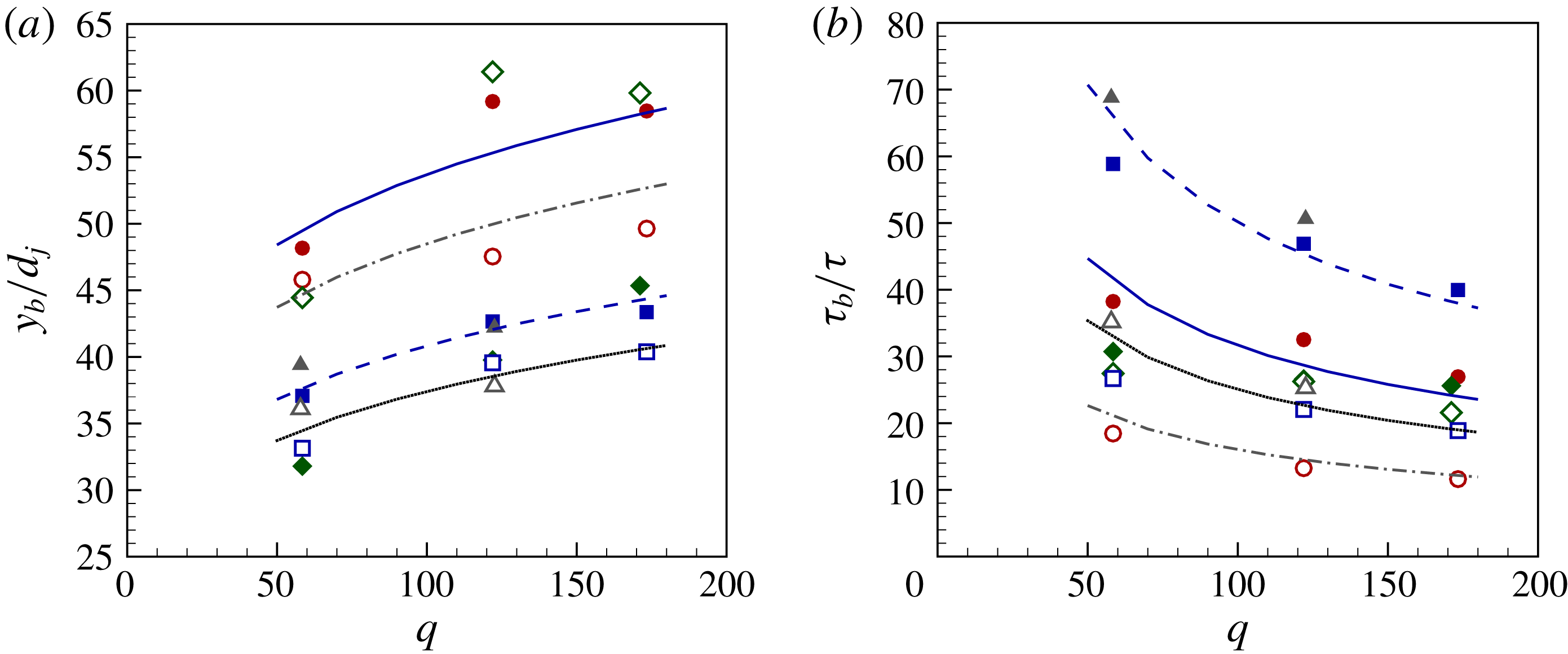Reference Wu, Kirkendall, Fuller and Nejad1997). The breakup height of the liquid jet of all examined cases in table 1 increases with increasing $q$ , as shown in figure 8(a). It is well known that the breakup height of a transverse liquid jet depends on the breakup regime. For both no-grid and grid test cases, the liquid jet in the enhanced capillary breakup mode (case No. 1) has a larger value at each specific $q$ compared to that of the liquid jet in the bag breakup regime (cases No. 3 and 4). For the two breakup regimes, nonetheless, it is revealed that increasing turbulence intensity (grid case) causes the liquid column to break up earlier. However, in case No. 2, as the liquid jet breaks up in the enhanced capillary regime when using a grid, its breakup height exhibits a similar trend to case No. 1, whereas that of the no-grid flow case (case No. 2), which breaks up in the bag breakup regime, is similar to cases No. 3 and 4. Figure 8(b) shows the breakup time, $\unicode[STIX]{x1D70F}_{b}$ , normalized by the integral time scale $\unicode[STIX]{x1D70F}$ for all the cases in table 1. It can be seen that, for each case, $\unicode[STIX]{x1D70F}_{b}/\unicode[STIX]{x1D70F}$ decreases with increasing $q$ as a result of a decrease in the liquid jet breakup time. Moreover, for both no-grid and grid test conditions, the breakup time of cases No. 3 and 4 shows a larger value than that of the case No. 1. For the two breakup regimes, it is also revealed that increasing turbulence intensity by using grid causes a decrease in the normalized breakup time by approximately 50 %. However, for case No. 2, it remains roughly unchanged.

Figure 8.

Effect of turbulent cross-airflow on the liquid jet’s (a) breakup height and (b) time for both no-grid (filled symbols) and grid (open symbols) conditions, for $We_{g}=3.1$ (● and ○), 4.82 (♦ and ♢), 5.88 (▪ and ▫) and 7.14 (▴ and ▵), where solid and dash-dot lines show the capillary breakup, and dashed and dotted lines show the bag breakup correlations for no-grid and grid conditions, respectively.

To predict the effect of the airflow turbulence properties on the liquid jet breakup height and time, empirical correlations are proposed in the enhanced capillary breakup and bag breakup regimes, which take into account the effect of the integral time scale of the airflow for both no-grid and grid test conditions. Following the analytical correlation proposed by Wu et al. (Reference Wu, Kirkendall, Fuller and Nejad1997) for the breakup height of a transverse liquid jet $y_{b}/d_{j}=C\sqrt{q}$ , where $C$ is a constant), $q$ was taken into account for predicting the breakup height of a liquid jet. Nonetheless, similar to the jet trajectory, it is clear that correlating the jet breakup height solely with $q$ is not able to account for the impact of the airflow’s turbulence. Therefore, in addition to $q$ , we propose to correlate the liquid jet breakup height with the integral time scale of the turbulent airflow. A nonlinear regression analysis is performed to develop the following correlations for the jet breakup height and its corresponding time within the range of the parameters examined in the present study (given in table 1):

(3.3) $$\begin{eqnarray}\displaystyle & \displaystyle y_{b}/d_{j}=C_{y}[(1/(\unicode[STIX]{x1D70F}_{b}/\unicode[STIX]{x1D70F}))q]^{0.15}, & \displaystyle\end{eqnarray}$$

(3.4) $$\begin{eqnarray}\displaystyle & \displaystyle \unicode[STIX]{x1D70F}_{b}/\unicode[STIX]{x1D70F}=C_{\unicode[STIX]{x1D70F}}t^{\ast }q^{-0.5}, & \displaystyle\end{eqnarray}$$

where, for the enhanced capillary and bag breakup regimes, $C_{y}$ is 16 and 11, and $C_{\unicode[STIX]{x1D70F}}$ is 316 and 500, respectively. In addition, $t^{\ast }$ which is defined as $t^{\ast }=(\unicode[STIX]{x1D70F}_{b}/\unicode[STIX]{x1D70F})/(\unicode[STIX]{x1D70F}_{b}/\unicode[STIX]{x1D70F})_{(no\text{-}grid)}$ is found to be 1 and 0.5 for the no-grid and grid test conditions studied in this paper. The correlation coefficient of the regression analysis is approximately 0.99, and the standard errors of the fits are 0.04 and 0.03 for the liquid jet breakup height and time, respectively. A comparison between the experimental liquid jet breakup height and time and their predictions using (3.3) and (3.4) is presented in figure 8. Taking into account the airflow turbulence integral time scale, in order to reflect the effect of the airflow’s turbulence properties, produces realistic predictions of the liquid jet’s breakup height and time for the range of parameters studied in the present paper.