





1. Introduction
Surface gravity waves affect the transport and mixing of scalars in the upper ocean. Waves generate a mean Lagrangian transport in the direction of propagation commonly known as the Stokes drift (Stokes Reference Stokes1847; van den Bremer & Breivik Reference van den Bremer and Breivik2018). Beyond affecting the mean transport directly, the Stokes drift also interacts with mean currents and turbulence, inducing Langmuir circulations which redistribute scalars beneath the surface (Craik & Leibovich Reference Craik and Leibovich1976). For random wave fields, the net drift velocity is often approximated as the linear superposition of each wave component (Kenyon Reference Kenyon1969). However, weak wave–wave interactions induce fluctuations in the local Stokes drift, which additionally cause scalars to spread diffusively (Herterich & Hasselmann Reference Herterich and Hasselmann1982). For inertial, non-neutrally buoyant particles, their transport deviates from the classic Stokes drift according to their shape, size and buoyancy (DiBenedetto et al. Reference DiBenedetto, Ouellette and Koseff2018, Reference DiBenedetto, Clark and Pujara2022). Beyond non-breaking waves, particles can ‘surf’ with the wave crests during a breaking event, translating at speeds significantly faster than the Stokes drift (Pizzo Reference Pizzo2017; Eeltink et al. Reference Eeltink, Calvert, Swagemakers, Xiao and van den Bremer2023). These studies demonstrate the importance of surface waves to scalar transport and dispersal in the ocean, however, less is known about the effect of waves on diffusion.
Large-eddy simulations have provided insight into wave-induced processes and their influence on material transport in the ocean mixed layer (see Chamecki et al. Reference Chamecki, Chor, Yang and Meneveau2019). However, these simulations do not typically resolve the unsteady wave orbital motion and instead utilise wave-averaged formulae to describe transport. While this approach can accurately represent the Stokes drift and its related processes, diffusion is generally assumed to be unchanged by the wave averaging. Law (Reference Law2000) questioned this assumption in the context of shear dispersion, comparing simulations of diffusive particles in phase-resolved waves with those in only the wave-averaged Stokes drift. They concluded that the Stokes drift was sufficient to describe scalar transport, suggesting that the wave motion has a negligible effect on diffusion; however, they only considered a narrow range of parameters. Furthermore, shear dispersion is a macroscopic process which tends to dominate diffusion over long time scales, making it difficult to isolate the true effects of waves on diffusion without considering it directly. DiBenedetto (Reference DiBenedetto2020) investigated the influence of wave motion on buoyant particles with a turbulent diffusivity, showing that the particle distribution oscillates as a function of wave phase, but did not consider any effect of the waves on diffusion. Perhaps one of the only studies to explicitly consider interactions between waves and diffusion is Jansons & Lythe (Reference Jansons and Lythe1998), who derived the Stokes drift for a Brownian particle. They showed that a large diffusivity inhibits scalars from coherently sampling the wave field, thereby reducing their Stokes drift. However, this only describes the influence of diffusion on advective transport. The opposite – the influence of advection on diffusive transport – has yet to be studied in the context of surface waves.
In regard to wave–turbulence interaction, wave orbital motion has received substantially more attention. Teixeira & Belcher (Reference Teixeira and Belcher2002) developed a rapid distortion model which demonstrates that progressive waves distort turbulence through two mechanisms: (i) the unsteady strain due to the wave orbital motion stretches and compresses the turbulence field, maximising the streamwise Reynolds stress under the wave crests and minimising it under the troughs – and conversely for the vertical Reynolds stress, and (ii) the Stokes drift shear gradually tilts vertical vortices in the direction of wave propagation. The latter mechanism is present in a wave-averaged framework, and its effects are cumulative and irreversible. The former mechanism is periodic although not perfectly sinusoidal under linear waves, suggesting correlation effects by the orbital motion later quantified by Xuan et al. (Reference Xuan, Deng and Shen2020), who found that phase correlations (which are typically unresolved) can account for up to 40 % of the turbulent kinetic energy production. These studies demonstrate that waves can influence turbulence beyond merely the Stokes drift, often doing so via the strain. Presumably, this wave-induced strain also distorts scalar fields, leading to the question: Does wave motion induce a net effect on diffusion?
Outside the context of ocean modelling, Press & Rybicki (Reference Press and Rybicki1981) theorised that internal wave motion influences diffusion and heat conduction in stars. They reached this conclusion by analysing the advection–diffusion equation in the Lagrangian frame, an approach which has since been used to study chaotic mixing (Thiffeault Reference Thiffeault2003), and to describe surfaces of minimal or maximal diffusion in Lagrangian coherent structures (Haller et al. Reference Haller, Karrasch and Kogelbauer2018). While many Lagrangian diffusion studies infer the particle trajectories from the Eulerian velocity fields, this approach can be problematic (analytically, not numerically) in the context of waves where the Eulerian and Lagrangian descriptions differ at the same order. Theoretical advances towards a fully Lagrangian description of steady surface gravity waves presents an alternative for addressing this issue (particularly Clamond Reference Clamond2007), which has recently been used to clarify the role of the Stokes drift in the kinematics and geometry of surface waves (Pizzo et al. Reference Pizzo, Lenain, Rømcke, Ellingsen and Smeltzer2023), how it relates to kinetic energy and vorticity (Blaser et al. Reference Blaser, Benamran, Bôas, Lenain and Pizzo2024) and its influence on the generation of surface waves by wind (Seitz et al. Reference Seitz, Freilich and Pizzo2026). However, this type of analysis has not yet been applied to diffusion.
The present study addresses this gap by developing a theoretical framework for the diffusive transport of scalars under surface gravity waves. A general description of diffusion in the Lagrangian frame is presented in § 2, which is then used to derive the diffusivity distortion for monochromatic progressive waves, standing waves and a wave spectrum in § 3. We also consider the influence of waves on the vertical distribution of buoyant particles in § 4, highlighting the importance of Lagrangian effects in the interpretation of models which are typically Eulerian. Finally, we compare our theory with numerical simulations in § 5, and finish with concluding remarks in § 6.
2. Scalar transport
To describe scalar transport, we consider a conserved passive scalar field
 $\phi (\boldsymbol{x},t)$
. In an incompressible flow with no sources or sinks, scalar conservation yields the Eulerian advection–diffusion equation
 \begin{align} \phi _{t}+ \boldsymbol{\nabla }\boldsymbol{\cdot }\left ( \boldsymbol{u}\phi \right ) = \kappa \boldsymbol{\nabla }\boldsymbol{\cdot }\left (\boldsymbol{D}\boldsymbol{\nabla }\phi \right ), \end{align}
where
 $\boldsymbol{\nabla }$
denotes the gradient operator with respect to physical space,
 $\boldsymbol{u}(\boldsymbol{x},t)$
is the Eulerian velocity field,
 $\boldsymbol{D}(\boldsymbol{x},t)$
is a general (dimensionless) diffusion-structure tensor accounting for possible anisotropy and spatio-temporal variation and
 $\kappa$
is a constant characteristic diffusivity. Here, subscripts denote partial derivatives and boldface is used to denote vectors and tensors. We now wish to express the advection–diffusion equation in the moving Lagrangian frame. This requires calculating the fluid particle trajectories
 $\boldsymbol{x}=\boldsymbol{x}(\boldsymbol{a},\tau )$
which represent a time-dependent, invertible mapping between label space
 $\boldsymbol{a}$
and physical space
 $\boldsymbol{x}$
. Particle labels can refer to initial positions, however, they can also be more arbitrarily defined so long as the mapping is one-to-one. This labelling freedom can be advantageous for interpretation, as will be discussed further in § 3. Here, we use
 $\tau$
to clarify that partial derivatives with respect to
 $\tau$
hold labels fixed, hereafter denoted by
 $\dot {(\;\;)}$
, whereas partial derivatives with respect to
 $t$
hold physical coordinates fixed. Following a particle trajectory, the advective term vanishes by construction and the scalar field is governed by the Lagrangian diffusion equation
 \begin{align} \dot {\phi }^\ell = \kappa \boldsymbol{\nabla }_{\boldsymbol{a}}\boldsymbol{\cdot }\big (\boldsymbol{D}^\ell \boldsymbol{\nabla }_{\boldsymbol{a}}\phi ^\ell \big ) . \end{align}
Here,
 $\boldsymbol{\nabla }_{\boldsymbol{a}}$
denotes the gradient taken with respect to the labels,
 $\phi ^\ell (\boldsymbol{a},\tau ) \equiv \phi (\boldsymbol{x}(\boldsymbol{a},\tau ),\tau )$
denotes the Lagrangian scalar field and the equivalent Lagrangian diffusivity is found from the chain rule
 \begin{align} \boldsymbol{D}^\ell (\boldsymbol{a},\tau ) = \boldsymbol{F}^{-1}\boldsymbol{D}(\boldsymbol{x}(\boldsymbol{a},\tau ),\tau )\boldsymbol{F}^{-T}, \end{align}
where
 $\boldsymbol{F}(\boldsymbol{a},\tau )\equiv \boldsymbol{\nabla }_{\boldsymbol{a}}\boldsymbol{x}$
is the deformation gradient, as in Press & Rybicki (Reference Press and Rybicki1981) and Haller et al. (Reference Haller, Karrasch and Kogelbauer2018). Most notably, even if the Eulerian diffusivity is uniform and isotropic, neither is necessarily true of the Lagrangian diffusivity, which depends on the deformation between the two frames. In the simplest case where the Eulerian diffusivity is isotropic such that
 $\boldsymbol{D} = \boldsymbol{I}$
, where
 $\boldsymbol{I}$
is the identity matrix, the Lagrangian diffusivity simplifies to
 $\boldsymbol{D}^\ell = \boldsymbol{C}^{-1}$
, where
 \begin{align} \boldsymbol{C}(\boldsymbol{a},\tau ) = \boldsymbol{F}^T\boldsymbol{F} \end{align}
is the right Cauchy–Green strain tensor – a representation of the deformation following a fluid element. Physically, the relationship between strain and diffusivity arises in the Lagrangian frame because the advection-induced deformation distorts (i) the local scalar gradient within a fluid parcel, and (ii) the area of the parcel available for diffusive flux.
An underappreciated feature of the Lagrangian approach is that the advective time scale now exists only within the Lagrangian diffusivity
 $\boldsymbol{D}^\ell$
. This naturally leads to a separation of scales where
 $\boldsymbol{D}^\ell$
varies much faster than
 $\boldsymbol{\nabla }_{\boldsymbol{a}}\phi ^\ell$
when the characteristic diffusivity is small (i.e. large Péclet number), as shown rigorously by Haller et al. (Reference Haller, Karrasch and Kogelbauer2018). Consequently,
 $\boldsymbol{\nabla }_{\boldsymbol{a}}\phi ^\ell$
is largely uncorrelated with the fast, advection-induced deformations present in
 $\boldsymbol{D}^\ell$
, implying that each can be averaged individually (over the advective time scale) without introducing unclosed terms. Thus, for the simplest case of a uniform and isotropic Eulerian diffusivity (
 $\boldsymbol{D}=\boldsymbol{I}$
) with small characteristic diffusivity
 $\kappa$
, as will be considered for this study, the leading-order evolution of
 $\phi ^\ell$
is governed by the advection-averaged strain. Finally, we note that the present study considers a generic down-gradient diffusive process which could represent either molecular or turbulent diffusion under an assumed turbulent diffusivity model. More sophisticated representations of turbulent mixing under waves may yield different results.
3. Lagrangian analysis
As made clear in § 2, to understand the influence of waves on diffusion, we must first analyse the wave-induced strain. We begin with permanent, progressive, monochromatic, two-dimensional, surface gravity waves of (small) amplitude
 $A$
and wavelength
 $\lambda$
in a water column of total depth
 $h$
. From this simplified scenario, we will find that the strain can be decomposed into multiple distinct mechanisms each with their own unique influence on diffusion. We will then use these results to extend our study to standing waves and a broadband wave spectrum.
3.1. Particle trajectories
Formally, the Lagrangian description of motion maps a particle from an initial position
 $\boldsymbol{x}_0$
at time
 $\tau _0$
to a later position
 $\boldsymbol{x}$
at time
 $\tau$
, where
 $\boldsymbol{x}_0$
and
 $\boldsymbol{x}$
lie on the same pathline and the trajectories
 $\boldsymbol{x}=\boldsymbol{x}(\boldsymbol{x}_0,\tau )$
are expressed as functions of the initial positions. However, it is generally insufficient to use initial positions as the independent variables when describing travelling waves of permanent form (Clamond Reference Clamond2007). This is made especially clear in the context of strain because initial positions set the relative ‘undeformed’ state via
 $\boldsymbol{C}(\boldsymbol{x}_0,\tau _0)\equiv \boldsymbol{I}$
. For permanent travelling waves, there is no reference position such that the fluid coincides with its quiescent state, and therefore can never be considered truly undeformed (see also Teixeira & Belcher Reference Teixeira and Belcher2002 § 3.2), which makes
 $\boldsymbol{C}$
difficult to interpret. Instead, it is convenient to consider the relabelling
 $(x_0,y_0)\to (a,b)$
such that the physical domain is mapped onto
 $-h\leqslant b\leqslant 0$
, where
 $b=0$
corresponds to the free surface and
 $b=-h$
corresponds to the sea bed, as in Clamond (Reference Clamond2007). Under this choice of labelling,
 $(a,b)$
represents the ‘rest position’ of the fluid in the absence of waves (Salmon Reference Salmon2020), and
 $\boldsymbol{C}$
now represents the wave-induced strain relative to a quiescent fluid. The Jacobian determinant of the transformation is then given by
 \begin{align} \mathcal{J} \equiv \det \boldsymbol{F}=x_ay_b-x_by_a, \end{align}
where the mapping is invertible given that
 $\mathcal{J}$
is sign-definite. The analysis in § 2 has already inherently chosen
 $\mathcal{J}=1$
such that infinitesimal areas are preserved between frames, however, it is noted that incompressibility only requires that
 $\mathcal{J}$
be time-independent (Pizzo et al. Reference Pizzo, Lenain, Rømcke, Ellingsen and Smeltzer2023).
We now assume that the fluid particle trajectories take the form
 \begin{align} x=a +U(b)\tau + \sum _{n=1}^{\infty }x_n(b)\sin \theta _n, \;\;\; y=b+Y(b) + \sum _{n=1}^{\infty }y_n(b)\cos \theta _n, \end{align}
as in Clamond (Reference Clamond2007) and Pizzo et al. (Reference Pizzo, Lenain, Rømcke, Ellingsen and Smeltzer2023). Here,
 $U(b)$
is the mean Lagrangian drift,
 $k=2\pi /\lambda$
is the wavenumber,
 $c$
is the phase speed and the wave phase
 $\theta _n=nk(a-(c-U(b))\tau )$
is necessarily Doppler-shifted by the drift to eliminate secular terms at higher orders. In contrast to known asymptotic expressions for the particle trajectories under surface waves, a more general form is preferable here to characterise each contribution to the fluid strain. It is also noted that (3.2) is chosen such that the wavelength is preserved between frames, enabling the simple wave-average
 $\left \langle \;\;\right \rangle =( {1}/{\lambda }) \int _{a}^{a+\lambda }(\;\;){\rm d}a'$
.
Finally,
 $Y(b)$
denotes the Lagrangian mean water level (i.e. mean elevation relative to the rest state), which in general differs from its Eulerian counterpart. This is because Eulerian wave-averaging integrates over points of equal spacing, whereas Lagrangian wave-averaging integrates over particles, which are unequally spaced in physical space (
 $x_a\neq 1$
). For surface gravity waves, particles tend to converge towards the crests and away from the troughs (see figure 1), and incompressibility is therefore maintained by a net vertical stretch supplied by the mean water level. Alternatively, the Lagrangian mean water level can be interpreted as the mean potential energy of fluid parcels balancing the mean kinetic energy due to the Lagrangian drift (Longuet-Higgins Reference Longuet-Higgins1986). A general expression for the mean water level can be found by substituting the trajectories (3.2) into (3.1) subject to the gauge choice
 $\mathcal{J}=1$
and wave averaging
 \begin{align} Y(b)=-\frac {1}{2}\sum _{n=1}^{\infty }nkx_ny_n, \end{align}
which also ensures that the Eulerian mean surface level is zero;
 $\langle yx_a\rangle |_{b=0}=0$
. Note that the Fourier modes
 $(x_n,y_n)$
are at most proportional to
 $A^n$
, meaning that
 $Y(b)$
is at most
 $\mathcal{O}(A^2)$
similar to the Lagrangian drift. Consequently, the leading-order mean water level is determined by the linear-order orbital motion.
3.2. Wave-averaged strain
As we attempt to interpret deformation in the Lagrangian frame, it is important to understand that the basis vectors
 $\boldsymbol{e}_a=(x_a,y_a)$
and
 $\boldsymbol{e}_b=(x_b,y_b)$
, which form the columns of
 $\boldsymbol{F}$
, are not necessarily horizontal and vertical, nor are they even orthogonal. Thus, the typical distinction between normal strain and shear strain generally becomes ill defined in label space. However, given trajectories of the form (3.2), it is readily shown that
 \begin{align} \left \langle \boldsymbol{e}_a\right \rangle =\left (1,\,0\right ),\;\;\;\;\left \langle \boldsymbol{e}_b\right \rangle =\left (U_b\tau ,\,1+Y_b\right ), \end{align}
which states that the wave-averaged basis vectors coincide with physical (i.e. Cartesian) space until acted upon by the Lagrangian drift. The ambiguity of the Lagrangian strain can therefore be reduced by decomposing the basis vectors into a wave-averaged component
 $\left \langle \boldsymbol{e}\right \rangle$
, which can be interpreted physically, and a fluctuating component
 $\boldsymbol{e}'\equiv \boldsymbol{e}-\left \langle \boldsymbol{e}\right \rangle$
, which accounts for correlations when the basis vectors are misaligned with physical space. Under this decomposition, the wave-averaged right Cauchy–Green strain is given by
 \begin{align} \left \langle \boldsymbol{C}\right \rangle =\underbrace {\begin{bmatrix} \left \langle \boldsymbol{e}_a\right \rangle \boldsymbol{\cdot }\left \langle \boldsymbol{e}_a\right \rangle & \left \langle \boldsymbol{e}_a\right \rangle \boldsymbol{\cdot }\left \langle \boldsymbol{e}_b\right \rangle \\[4pt] \left \langle \boldsymbol{e}_b\right \rangle \boldsymbol{\cdot }\left \langle \boldsymbol{e}_a\right \rangle & \left \langle \boldsymbol{e}_b\right \rangle \boldsymbol{\cdot }\left \langle \boldsymbol{e}_b\right \rangle \end{bmatrix}}_{\boldsymbol{C}^m}+\underbrace {\begin{bmatrix} \left \langle \boldsymbol{e}_a' \boldsymbol{\cdot }\boldsymbol{e}_a'\right \rangle & \left \langle \boldsymbol{e}_a' \boldsymbol{\cdot }\boldsymbol{e}_b'\right \rangle \\[4pt] \left \langle \boldsymbol{e}_b' \boldsymbol{\cdot }\boldsymbol{e}_a'\right \rangle & \left \langle \boldsymbol{e}_b' \boldsymbol{\cdot }\boldsymbol{e}_b'\right \rangle \end{bmatrix}}_{\boldsymbol{C}^f} \!. \end{align}
Here, the diagonals and off-diagonals of
 $\boldsymbol{C}^m$
can be interpreted as normal and shear respectively (either for small
 $\tau$
or asymptotically), however, these characterisations cannot be applied to the entries of
 $\boldsymbol{C}^f$
despite the fact that they are additive. For example, the Lagrangian drift, whose gradient is nominally interpreted as a shear strain, will partially align with
 $\boldsymbol{e}_a'$
and
 $\boldsymbol{e}_b'$
and is therefore sometimes ‘seen’ as normal by the fluctuating axes. This nuance is not appreciated by a direct calculation of
 $\left \langle \boldsymbol{C}\right \rangle$
, highlighting that one must be careful when interpreting deformation in the Lagrangian frame.
From the wave-averaged basis vectors (3.4), it is easily shown that
 \begin{align} \boldsymbol{C}^m=\begin{bmatrix} 1 & U_b\tau \\[4pt] U_b\tau & \left (1+Y_b\right )^2+U_b^2\tau ^2 \end{bmatrix}\!, \end{align}
valid to all orders of amplitude. Here, we observe that there is a mean vertical stretch due to the depth dependence of the mean water level, and a cumulative shear strain due to the Lagrangian drift. In the context of turbulence, the off-diagonals of (3.6) are immediately recognised as the fully Lagrangian analogue of the second Craik-Leibovich mechanism: the cumulative tilting of vertical vortices (here, material lines) in the direction of wave propagation by the Lagrangian drift (Craik & Leibovich Reference Craik and Leibovich1976; Teixeira & Belcher Reference Teixeira and Belcher2002). We now calculate the correlation terms
 $\boldsymbol{C}^f$
. The steps are more involved and are therefore provided in Appendix A, however, the final result is rather simple
 \begin{align} \boldsymbol{C}^f= \frac {U+{\varGamma }}{c-U}\boldsymbol{C}^m + \mathcal{O}(A^4), \end{align}
where
 ${\varGamma }(b)\sim A^2$
is the circulation per unit wavelength (i.e. enclosed vorticity, note we have not assumed irrotational). Given that
 $\boldsymbol{C}^f$
is proportional to
 $\boldsymbol{C}^m$
, its net contribution cannot be a stretching or compressing mechanism, but rather is a dilatation which maintains the choice of
 $\mathcal{J}$
for the instantaneous strain
 $\boldsymbol{C}$
, since
 $\det \boldsymbol{C}\equiv \mathcal{J}^2$
(note,
 $\det \boldsymbol{C}\neq \det \left \langle \boldsymbol{C}\right \rangle )$
. This is made further apparent by the fact that the coefficient of (3.7) does not comprise any terms which produce material deformation, namely the lack of any gradients. As such,
 $\boldsymbol{C}^f$
does not possess any mechanism which can physically affect diffusion (i.e. it does not stretch, squish, or shear a fluid parcel) and is therefore only relevant if one wishes to obtain solutions to the label space diffusion equation (2.2). However, this is unnecessary given that any changes to the diffusivity in Cartesian space can be measured directly, as will be shown in § 5. Note that this interpretation would not be apparent had we used explicit asymptotic trajectories instead of a general form for (3.2), which would lead to ambiguous characterisations of the strain and thus the diffusion.
Additionally, we make the physical observation that the fluid motion must be unaffected by the presence of (or lack thereof) passive scalars. Given the definition
 $\boldsymbol{C}^f= \langle {\boldsymbol{F}'}^T\boldsymbol{F}' \rangle$
, we see that
 $\boldsymbol{C}^f$
quantifies the correlation between the deformation of a fluid parcel and the deformation of the local concentration gradient rather than quantifying the fluid strain directly. In contrast,
 $\boldsymbol{C}^m=\langle \boldsymbol{F}\rangle ^T\langle \boldsymbol{F}\rangle$
quantifies the combined effect when a fluid parcel and the concentration gradient are subjected to the same deformation independently, which is more representative of the actual fluid strain. While there likely exists alternate interpretations for what
 $\boldsymbol{C}^f$
represents physically, we will find in § 5 that its effects are indeed absent in our numerical results.
3.3. Wave-averaged diffusivity
Upon identifying
 $\boldsymbol{C}^m$
as the physically relevant term for the diffusion in Cartesian space, we can now begin to associate its components with various diffusion mechanisms, starting by re-expressing (3.6) as
 \begin{align} \boldsymbol{C}^m= \begin{bmatrix} 1 & U_b\tau \\[5pt] U_b\tau & 1+U_b^2\tau ^2 \end{bmatrix} + \begin{bmatrix} 0 & 0 \\[5pt] 0 & 2Y_b+Y_b^2 \end{bmatrix}\!. \end{align}
Written this way, we observe that the first term is identical to the Lagrangian strain of a simple shear flow;
 $x=a+U(b)\tau$
and
 $y=b$
, corresponding to the Eulerian velocity
 $\boldsymbol{u}= (U(y),0 )$
. It has been well known since Taylor (Reference Taylor1953) that scalars in a shear flow experience a macroscopic streamwise diffusion due to variations in the local scalar velocity relative to the bulk speed of the concentration field. This process is commonly known as shear dispersion, and it is typically quantified by an effective Eulerian diffusivity calculated from the aforementioned velocity variations. In general, it is difficult to translate Taylor’s analysis to the Lagrangian frame because the label variables
 $(a,b)$
cannot describe a fixed cross-section in physical space and therefore cannot define a cross-sectional average, which is central to classic shear dispersion theory. It is for this reason that analytical studies of wave-induced shear dispersion have previously used techniques (e.g. homogenisation, generalised Lagrangian mean theory) to recover the drift in an Eulerian or quasi-Eulerian frame (see e.g. Yan et al. Reference Yan, Zou and You2022), however, we can still appreciate that the drift terms in (3.8) pertain to the same physical mechanism.
We now reach the crux of our study, which is that there is still a non-cumulative normal strain from the mean water level, distinguishing the net transport by surface waves from that of a basic shear flow. Simply put, a fluid parcel under phase-resolved waves is, on average, vertically elongated and therefore has more area available for horizontal flux than in the scenario where only the drift is considered. This effect, hereafter referred to as ‘distortion’, is local, compared with shear dispersion which is a relative, macroscopic diffusion. Most notably, distortion is present for any non-zero characteristic diffusivity (
 $\kappa \gt 0$
) and is independent of the scalar concentration field. In contrast, both the presence and form of shear dispersion depend on the vertical scalar distribution. For example, consider a scalar field constrained to a material line of constant
 $b$
, such as the free surface. Since each scalar is fixed to the same material depth, the velocity field as seen by the scalars is no longer sheared, i.e. the velocity of any individual scalar is identical to the bulk speed of the concentration field, hence there cannot be any shear dispersion. However, the scalars still feel the axial stretching and squashing from the waves and thus experience an enhanced diffusion along the material line given by
 \begin{align} \kappa \big \langle D^\ell _{11}\big \rangle =\kappa \left (1+\mathcal{D}(b)\right ), \end{align}
where
 $\mathcal{D}(b)=2Y_b+Y_b^2$
is the wave-averaged distortion (obtained from the cofactor of (3.8) with
 $U_b=0$
given that we are neglecting
 $\boldsymbol{C}^f$
). It is precisely this thought experiment which we will use to measure the distortion numerically in § 5. In the language of generalised Lagrangian mean theory (i.e. Lagrangian = Eulerian + Stokes), distortion essentially represents a ‘Stokes correction’ to the horizontal diffusivity (note, distortion is purely horizontal;
 $\kappa \left \langle D_{22}^\ell \right \rangle =\kappa$
). That is, distortion is to the particle diffusivity what Stokes drift is to the particle velocity. Thus, (3.9) is the equation of interest for practical modelling efforts, as shear dispersion will already be accounted for by any model which parametrises the advection due to the Stokes drift.
Finally, although not considered here, any general Eulerian diffusivity tensor
 $\boldsymbol{D}$
will distort according to (2.3) and can be analysed following an analogous procedure. In the special case where
 $\boldsymbol{D}(\boldsymbol{x}(\boldsymbol{a},\tau ),\tau )= \boldsymbol{C}$
, the distortion will cancel the anisotropy and spatio-temporal dependence of
 $\boldsymbol{D}$
, and the scalar field will behave as if it had a constant diffusivity. This is, in essence, what non-phase-resolving models are unknowingly imposing when assuming a constant diffusivity in a wave-averaged frame.


3.4. Asymptotic analysis
We can now consider asymptotic expressions for the particle trajectories to quantify how the unsteady strain and associated mean water level affect both the instantaneous and wave-averaged diffusion. Since the leading-order contribution to the mean water level is set by the linear-order orbital motion, we can simply consider the particle trajectories given by linear wave theory
 \begin{align} x & = a - A \frac {\cosh k(b+h)}{\sinh kh}\sin k(a-c\tau ), \\[-12pt] \nonumber \end{align}
 \begin{align} y & = b + A \frac {\sinh k(b+h)}{\sinh kh}\cos k(a-c\tau ). \\[10pt] \nonumber \end{align}
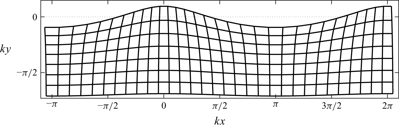
The deformation due to the orbital motion (3.10a , b ) is visualised in figure 1, where we observe vertical elongation under the wave crests and compression under the troughs, with the opposite trend in the horizontal. To demonstrate the phase variation in the diffusion due to this oscillating strain, we calculate the normal diffusivities to linear order
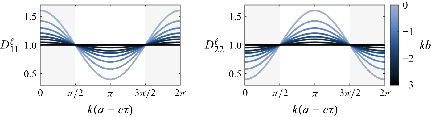
 \begin{align} \boldsymbol{D}^\ell (\boldsymbol{a},\tau )= \begin{bmatrix} 1 + 2Ak\frac {\cosh k(b+h)}{\sinh kh}\cos k(a-c\tau ) & \\ & 1-2Ak\frac {\cosh k(b+h)}{\sinh kh}\cos k(a-c\tau ) \end{bmatrix} \!. \end{align}
At this order, we can characterise
 $k(a-c\tau ) \in [0,{\pi }/{2} ] \cup [{3\pi }/{2}, 2\pi ]$
as a crest, and
 $k(a-c\tau ) \in [ {\pi }/{2}, {3\pi }/{2} ]$
as a trough. Plotted in figure 2, we find that the horizontal diffusivity
 $D^\ell _{11}$
is maximised under the crests where there is the most area available for horizontal flux as well as the steepest horizontal concentration gradient, and minimised under the troughs where there is the least flux area and the weakest concentration gradient. The trend is reversed for the vertical diffusivity
 $D^\ell _{22}$
, which is minimised under the crests and maximised under the troughs. When contrasted with the deformation shown in figure 1, these trends clearly reflect the inverse relationship between strain and diffusion.
Phase variation of the normal diffusivities (3.11) for
 $kh\to \infty$
and
 $Ak = 0.3$
. Shaded and unshaded areas represent crests and troughs, respectively.

To calculate the wave-averaged distortion, it can be seen from (3.3) and (3.9) that
 $\mathcal{D}(b)=-k(x_1y_1)_b$
to leading order. Hence, we substitute
 $x_1$
and
 $y_1$
from the linear orbital-motion (3.10a
,
b
) to obtain
 \begin{align} \mathcal{D}(b)=A^2k^2\frac {\cosh 2k(b+h)}{\sinh ^2kh}+\mathcal{O}(A^4), \end{align}
which shows that the horizontal diffusion is most enhanced under steep and shallow waves, and decays rapidly with depth. Note that we need not consider the second-order harmonics present in finite-depth waves when calculating the distortion, as these terms have no net effect at the order we are considering.
3.4.1. Standing waves
Next, we consider a standing wave of amplitude
 $A$
by superimposing two identical but opposing waves given by (3.10a
,
b
) each with amplitude
 $A/2$
and separated by a phase shift of
 $2\beta$
. The resultant trajectory is simplified using sum-to-product identities
 \begin{align} x & = a - A \frac {\cosh k(b + h)}{\sinh kh} \sin (ka - \beta )\cos (kc\tau - \beta ), \\[-12pt] \nonumber \end{align}
 \begin{align} y & = b + A \frac {\sinh k(b + h)}{\sinh kh} \cos (ka - \beta )\cos (kc\tau - \beta ). \\[10pt] \nonumber \end{align}
Similar to travelling waves, the Lagrangian mean water level can still be calculated such that
 $\mathcal{J}=1$
at second order (note, standing waves must additionally be time averaged over one cycle), and it is readily shown that the distortion for a standing wave is given by
 \begin{align} \mathcal{D}_{\text{st}}(b)=\frac {1}{2}A^2k^2\frac {\cosh 2k(b+h)}{\sinh ^2kh}+\mathcal{O}(A^4). \end{align}
Thus, the distortion under a standing wave is half that of a travelling wave of the same amplitude, similar to the result obtained by Knobloch (Reference Knobloch1991) via homogenisation (an Eulerian method). The presence of distortion under standing waves also explicitly shows its distinction from shear dispersion given that standing waves have no net drift. Finally, we observe that (3.14) is twice the distortion of a travelling wave with amplitude
 $A/2$
, demonstrating that the distortion effect is additive when waves can be superimposed.
3.4.2. Wave spectra
Lastly, given that the ocean is typically forced by a wave spectrum, we calculate the distortion due to an irregular wave field. We consider a one-dimensional energy spectrum
 $S(k)$
with its integral defined as the variance of the free surface displacement
 \begin{align} \overline {\eta ^2} = \int _{-\infty }^{\infty } S(k){\rm d}k, \end{align}
where
 $\eta (x,t) = y(a(x,t),0,t)$
is the Eulerian free surface, and the overline denotes an ensemble average. It is frequently assumed that wave–wave interactions are negligible and that the wave field can be treated as a linear sum of monochromatic waves (Kenyon Reference Kenyon1969). Under this assumption, the ensemble-mean distortion is given by the continuous sum of each wave component
 \begin{align} \mathcal{D}_{\text{sp}}(b) = \int _{-\infty }^{\infty }2k^2S(k)\frac {\cosh 2k(b + h)}{\sinh ^2kh}\,{\rm d}k + \mathcal{O}(A^4), \end{align}
showing that the net distortion can be easily recovered for a known wave spectrum. This is analogous to how the total Lagrangian drift is often calculated for irregular waves, however, recent studies show that this approach can under-predict the drift when the wave field becomes locally steep (Blaser et al. Reference Blaser, Lenain and Pizzo2026), in which case we would expect the higher-order corrections to (3.16) to become important as well.
4. Influence of the mean water level on buoyant particle distributions
The previous section demonstrates that waves enhance the mean horizontal diffusivity of passive scalars. This effect is purely horizontal, suggesting that the vertical concentration remains unchanged by the waves on average. However, the mean displacement of particles is still influenced by the Lagrangian mean water level, which may be important to consider in modelling efforts. In this section, we investigate the influence of the mean water level on buoyant particle distributions (e.g. microplastics, oil droplets, bubbles), in particular demonstrating how it can skew the interpretation of microplastics transport models.
First, we consider a quiescent, infinitely deep fluid containing buoyant, inertialess particles with constant vertical rise velocity
 $v_r$
and diffusivity
 $\kappa$
. For a horizontally uniform concentration field at equilibrium, the Eulerian advection–diffusion equation (2.1) reduces to
 \begin{align} v_r \phi = \kappa \frac {\partial \phi }{\partial y}, \end{align}
given a no-flux condition at the free surface
 $y=0$
. Note that an Eulerian approach must be used here because there is no flow and the particles can no longer be approximated as fluid tracers. Solving the differential equation (4.1), the particle distribution is given by an exponential decay
 \begin{align} \phi (y)=\phi _0\exp \left (\frac {y}{L_m}\right )\!, \end{align}
where
 $\phi _0$
is the concentration at the free surface and
 $L_m\equiv \kappa /v_r$
is a ‘mixing length scale’, as in Kukulka et al. (Reference Kukulka, Proskurowski, Morét-Ferguson, Meyer and Law2012) and DiBenedetto (Reference DiBenedetto2020). Note that we are using constant parameters here for simplicity, but our analysis can easily be extended to scenarios with a depth-varying rise velocity and/or diffusivity. Equation (4.2) represents a simplified ‘wind-mixing model’ that is widely used to study ocean microplastics, where it is typically assumed that the wave motion itself does not have any net influence on the vertical particle distribution. To better understand the mixing length scale
 $L_m$
, it can be verified from (4.2) that
 \begin{align} \int _{-\infty }^{0} y\phi (y)\,{\rm d}y\bigg /\int _{-\infty }^{0} \phi (y)\,{\rm d}y=-L_m, \end{align}
meaning that physically,
 $L_m$
corresponds to the centroid of the distribution, i.e. the mean particle depth in a quiescent fluid.
We now consider the effect of waves where both the rise velocity and diffusivity are assumed to be slow relative to the wave motion. Using the mean water level from § 3.4 as
 $kh\to \infty$
, the mean particle depth is, on average, mapped to
 \begin{align} -L_m'= -L_m +\frac {1}{2}A^2ke^{-2kL_m} + \mathcal{O}(A^4), \end{align}
where
 $L_m'$
is the centroid inherently considered when the wind-mixing model is applied to real data, but is otherwise mistaken as
 $L_m$
. From this relationship, we clearly see that the centroid relative to the Eulerian mean surface
 $(y=0)$
is different in the presence of waves than in the absence of waves. We can characterise the relative importance of this effect by analysing
 $kL_m$
, which characterises how deep particles are mixed relative to the decay scale of the waves:
 $kL_m \gg 1$
implies that diffusion dominates over buoyancy and particles are mixed far beneath the surface, whereas
 $kL_m \ll 1$
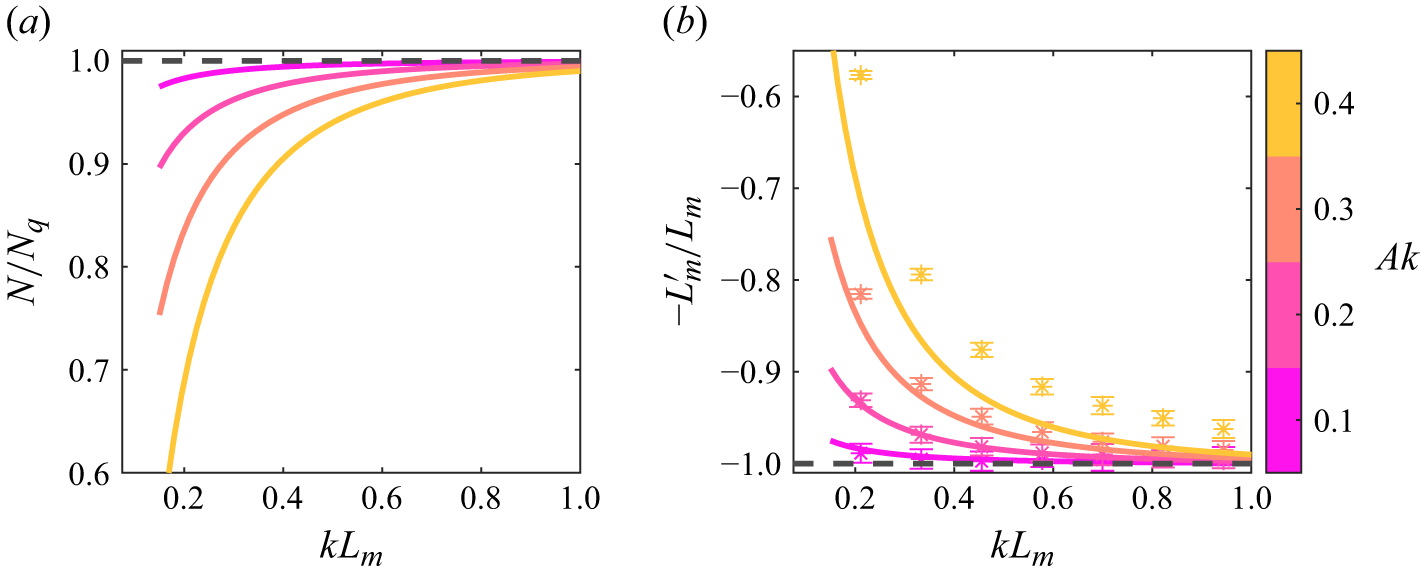
implies that the particles are strongly buoyant and concentrated near the surface where the waves are most important. To support our discussion, we compare the adjusted mean particle depth (4.4) with numerical simulations of buoyant, diffusive particles under deep water waves (methods discussed in § 5). Shown in figure 3, we observe that the shift in mean particle depth can be mostly explained by the Lagrangian mean water level, implying that the particle rise velocity and vertical diffusivity are largely unaffected by the waves, although kinematic enhancements to the rise velocity were considered by DiBenedetto et al. (Reference DiBenedetto, Clark and Pujara2022).
We now discuss two examples which illustrate the influence of the mean water level. First, surface measurements are often used to extrapolate the total number of microplastic particles beneath the surface (see e.g. Kukulka et al. Reference Kukulka, Proskurowski, Morét-Ferguson, Meyer and Law2012). However, the concentration with centroid
 $L'_m$
encloses a different area than that with centroid
 $L_m$
. This is readily shown by calculating the ratio of the total number of particles
 $N$
from the profile with centroid
 $L_m'$
, to the number of particles
 $N_q$
from the profile with centroid
 $L_m$
(which can be taken as the ground truth)
 \begin{align} \frac {N}{N_q}=\int _{-\infty }^{0}\exp \left (\frac {y}{L_m'}\right ){\rm d}y\bigg /\int _{-\infty }^{0}\exp \left (\frac {y}{L_m}\right ){\rm d}y=\frac {L_m'}{L_m}. \end{align}
As demonstrated in figure 3, the estimated particle count
 $N$
under-predicts the actual count
 $N_q$
which would be observed for the same particles in the absence of waves – in some cases by a significant amount. Second, the rise velocity and/or diffusivity are sometimes inferred from concentration measurements. For example, Brunner et al. (Reference Brunner, Kukulka, Proskurowski and Law2015) calculated a concentration profile analogous to (4.2) using a depth-dependent diffusivity to parameterise the effects of Langmuir turbulence. They then used the rise velocity
 $v_r$
as a fitting parameter to compare the theoretical distribution with observations. In this context, we see from (4.4) that the wave motion raises the centroid of the distribution, which would lead one to conclude that the particle rise velocity is higher than in reality.
Estimated total particle count and the wave-induced change in the mean particle depth. (a) Ratio of the total particle count
 $N/N_q$
as a function of
 $kL_m$
. (b) Adjusted mean particle depth normalised by the quiescent case. Solid lines are equation (4.4) and dots are numerical data, where the error bars represent one standard deviation of the ensemble-mean time series. In both plots, the dashed line denotes the no-waves case.

Figure 3. Long description
The image contains two line graphs. Panel A shows the ratio of the total particle count as a function of kLm. The x-axis is labeled kLm and the y-axis is labeled N/Nq. The graph includes multiple colored lines representing different values of Ak, with a dashed line indicating the no-waves case. Panel B shows the adjusted mean particle depth normalized by the quiescent case as a function of kLm. The x-axis is labeled kLm and the y-axis is labeled −L’/Lm. This graph also includes multiple colored lines and a dashed line for the no-waves case. Both graphs use solid lines to represent equation (4.4) and dots to represent numerical data, with error bars indicating one standard deviation of the ensemble-mean time series.
Finally, we rescale our dimensionless parameters to estimate the relevant magnitude for the rise velocity. From figure 3, we find that the mean water level is generally important for
 $kL_m \lt 1$
, or alternatively
 $v_r \gt \kappa k$
. Thus, for a typical turbulent diffusivity
 $\kappa \sim 10^{-4}$
m
 $^2$
s−1 and wavelength
 $\lambda \sim 100$
m, we find that the mean water level will be important for
 $v_r \gt 1$
mm s−1, which applies to a significant range of ocean plastics (see DiBenedetto et al. Reference DiBenedetto, Donohue, Tremblay, Edson and Law2023).
5. Numerical simulations
To validate our theory, we perform a set of phase-resolving numerical simulations. We characterise the scalar field by a discrete number of particles which are iterated through an Eulerian velocity field and prescribed a constant diffusivity
 $\kappa$
. Using this approach, the Lagrangian drift, mean water level and diffusivity distortion emerge naturally in the long-time statistics. The particle motion is governed by a two-dimensional system of stochastic differential equations
 \begin{align} {\rm d}\boldsymbol {x} = \boldsymbol {u}(t){\rm d}t + \sqrt {2\kappa }{\rm d}\boldsymbol {W}. \end{align}
Here,
 ${\rm d}\boldsymbol {W}=\boldsymbol{\xi }\sqrt {{\rm d}t}$
is a Brownian motion increment with zero mean and variance
 ${\rm d}t$
, and
 $\boldsymbol{\xi } \sim \mathcal{N}(0,1)$
is a normally distributed random variable. The particle motion (5.1) is iterated using a fourth-order Runge–Kutta scheme with a time step defined by the wave period
 ${\rm d}t=T_w/200$
(peak period for wave spectra) to ensure that the orbital motion is well resolved. In all cases, the diffusivity is constrained to
 $\kappa \lesssim cA^2k$
such that the diffusion is sufficiently slow compared with the orbital motion. This is still larger than typical turbulent diffusivities observed under wind-driven waves (see Anis & Moum Reference Anis and Moum1994), however, the results do not depend on
 $\kappa$
given that the diffusion is ‘slow enough’, and increasing the diffusivity helps particles reach steady state quicker, thereby reducing computational cost. Lastly, we note that our results are taken at steady state and therefore do not depend on the initial conditions.
5.1. Diffusivity distortion
To isolate distortion, we must first eliminate any contributions from the drift-induced shear dispersion. As outlined in § 3.3, this can be achieved by constraining particles to a material surface of constant
 $b$
after every time step such that each particle has the same mean drift. While the surface corresponding to
 $b=0$
is simply the free surface
 $\eta (x,t)$
, measuring distortion as a function of depth requires a more generalised expression which can be found by inverting the horizontal trajectory
 $x(a,b,\tau )$
iteratively to obtain
 $a=a(x,t;b)$
and then substituting into
 $y(a,b,\tau )$
. For simplicity, we will only perform this calculation for deep water monochromatic waves, whereas particles will be constrained to the free surface for finite-depth, standing and irregular waves. Upon obtaining expressions for the desired boundary conditions, the particle motion is simulated until steady state is reached, and the diffusivity is calculated from the mean squared displacement (where the distortion is found by subtracting off the characteristic diffusivity, per equation (3.9))
 \begin{align} \mathcal{D}(b)= \lim _{t\to \infty }\frac {1}{2\kappa }\frac {{\rm d}\overline {x^2(t)}}{{\rm d}t}-1. \end{align}
To reduce noise and average out the orbital motion, the particle trajectories are smoothed first using a moving average with a width of one wavelength, then repeated with a width of two wavelengths, where the error is quantified through the standard deviation of the ensemble-mean time series.
5.1.1. Travelling waves
For monochromatic, progressive waves of arbitrary depth, the Eulerian velocity field and free surface are given by second-order wave theory
 \begin{align} u & = Akc \frac {\cosh k(y+h)}{\sinh kh}\cos \theta + A^2k^2c\frac {3\cosh 2k(y+h)}{4\sinh ^4 kh}\cos 2\theta , \\[-12pt] \nonumber \end{align}
 \begin{align} v & = Akc \frac {\sinh k(y+h)}{\sinh kh}\sin \theta + A^2k^2c\frac {3\sinh 2k(y+h)}{4\sinh ^4 kh}\sin 2\theta , \\[-12pt] \nonumber \end{align}
 \begin{align} \eta & = A\cos \theta + A^2k\frac {3-\tanh ^2 kh}{4\tanh ^3 kh}\cos 2\theta , \\[10pt] \nonumber \end{align}
where
 $\theta = k(x-ct)$
. In all cases, the wave steepness was varied in the range
 $0.1\leqslant Ak\leqslant 0.4$
so as not to exceed typical breaking limits. To measure the influence of finite-depth waves, particles were constrained to the free surface and the total depth was varied in the range
 $\pi /4 \leqslant kh \leqslant \pi$
, after which the waves are effectively infinitely deep. To measure the depth profile, particles were constrained to the material surface
 \begin{align} y(x,t;b)=b+Ae^{kb}\cos \theta + \frac {1}{2}A^2ke^{2kb}\cos 2\theta +\mathcal{O}(A^3), \end{align}
obtained from the aforementioned inversion procedure. The material depth was varied in the range
 $0\leqslant b\leqslant -\pi /2$
, and
 $10\,000$
trajectories were simulated for
 $500$
wave periods given each
 $b$
or
 $kh$
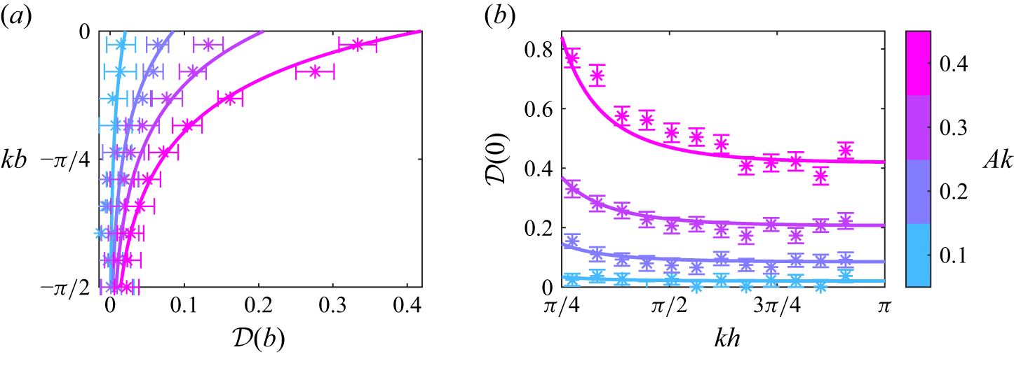
input. The distortion was then calculated from (5.2), with the results shown in figure 4. Here, we find good alignment between the theoretical expression (3.12) and the numerical results, with the largest inaccuracies occurring near the free surface and for large wave steepness.
Diffusivity distortion for monochromatic progressive waves. (a) Distortion depth profiles in deep water waves. (b) Distortion at the free surface as a function of the total water depth
 $kh$
. Solid lines are (3.12) and dots are numerical data where the error bars represent one standard deviation of the ensemble-mean time series.

5.1.2. Standing waves
To construct a standing wave of steepness
 $Ak$
, we superimpose two identical but opposing waves given by (5.3) each with steepness
 $Ak/2$
. Here,
 $20\,000$
trajectories were simulated for
 $500$
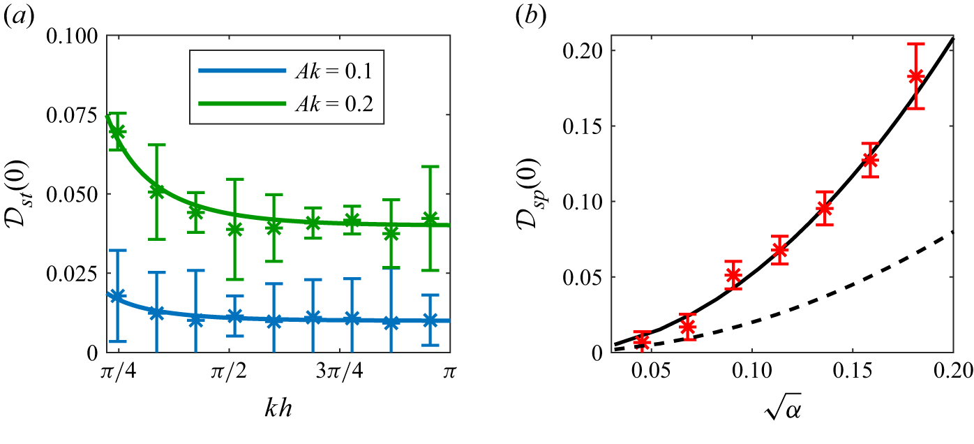
wave periods, and the distortion was again calculated from (5.2). Results for standing waves are shown in figure 5, where we observe that the distortion under a standing wave is half that of the travelling wave shown in figure 4, and again find that the numerical data align well with the theoretical prediction (3.14).
Diffusivity distortion at the free surface for standing waves and irregular waves. (a) Distortion under standing waves as a function of total water depth
 $kh$
. (b) Distortion under irregular waves as a function of effective wave steepness
 $\sqrt {\alpha }$
. Solid lines are (3.14) and (5.8), (a) and (b), respectively, and the dots are numerical data where the error bars represent one standard deviation of the ensemble-mean time series. The dashed line is a monochromatic wave of steepness
 $Ak = \sqrt {\alpha }$
for reference.

5.1.3. Irregular waves
Lastly, we consider deep water irregular waves generated from a Joint North Sea Wave Project (JONSWAP) spectrum (Hasselmann et al. Reference Hasselmann1973). The energy spectrum is given by
 \begin{align} S(\omega ) = \alpha g^2 \omega ^{-5}\exp \left [-\frac {5}{4}\left (\frac {\omega _p}{\omega }\right )^4\right ]\gamma ^{\exp \left [-\frac {(\omega /\omega _p - 1)^2}{2\sigma ^2}\right ]}, \;\;\; \sigma = \begin{cases} 0.07 & \omega \leqslant \omega _p, \\ 0.09 & \omega \gt \omega _p, \end{cases} \end{align}
where
 $\gamma = 3.3$
is the peak enhancement factor,
 $\omega _p$
is the peak frequency,
 $g$
is the gravitational acceleration and
 $\alpha$
is a dimensionless constant. We construct the wave field from
 $500$
individual wave components with frequencies in the range
 $0.5 \leqslant {\omega }/{\omega _p} \leqslant 4$
, and the discrete wave amplitudes are related to the energy spectrum via
 \begin{align} A_n^2=2S(\omega _n)\Delta \omega . \end{align}
The velocity field and free surface are then given by the superposition of each wave component
 \begin{align} u & = \sum _n \omega _n A_n e^{k_n y}\cos (k_n x - \omega _n t + \varphi _n), \\[-12pt] \nonumber \end{align}
 \begin{align} v & = \sum _n \omega _n A_n e^{k_n y}\sin (k_n x - \omega _n t + \varphi _n), \\[-12pt] \nonumber \end{align}
 \begin{align} \eta & = \sum _n A_n\cos (k_n x - \omega _n t + \varphi _n), \\[10pt] \nonumber \end{align}
where
 $\varphi _n$
is a uniformly distributed random phase shift and the wavenumbers are given by the dispersion relation
 $k_n=\omega _n^2/g$
.
To be consistent with the energy spectrum (5.5), we express the distortion (3.16) in terms of frequency, which at the free surface is given by
 \begin{align} \mathcal{D}_{{sp}}(0) = \int _{0}^{\infty }4g^{-2}\omega ^4S(\omega ) {\rm d}\omega . \end{align}
If we compare the irregular distortion (5.8) with the monochromatic distortion (3.12), it becomes apparent that
 $\alpha$
plays a similar role for the wave spectrum (5.5) that
 $A^2k^2$
does for a monochromatic wave. Thus, we consider
 $\sqrt \alpha$
as our control variable, analogous to varying the steepness of a monochromatic wave. For each
 $0.04\leqslant \sqrt \alpha \leqslant 0.2$
, a total of
 $50\,000$
trajectories were simulated for
 $750$
peak wave periods, and the distortion was again calculated from (5.2). Results for irregular waves are shown in figure 5 alongside a monochromatic wave of steepness
 $Ak=\sqrt {\alpha }$
to show the difference. From this comparison, we find that the wave spectrum induces a much greater distortion than monochromatic waves, more than doubling the relative effect within the given parameter space and again showing that the numerical data are well predicted by our theory.
5.2. Mean depth of buoyant particles
To measure the mean effect of waves on buoyant particle distributions, we simulate the steady-state mean depth of diffusive, buoyant particles. We consider monochromatic progressive waves governed by (5.3) as
 $kh\to \infty$
with an added constant rise velocity
 $v_r$
to (5.1). In these simulations, particles are no longer constrained to a specific material surface and are free to distribute throughout the water column. The transport due to diffusion and buoyancy are calculated in sequence, where the boundary condition is as follows: (i) after a diffusive step, a particle which is above the free surface is reflected back, (ii) after a buoyant step, a particle which is above the free surface is placed back at the free surface. This is to mimic the no-flux boundary condition from § 4. Here, we again varied the wave steepness in the range
 $0.1\leqslant Ak \leqslant 0.4$
, and we simulated
 $10\,000$
trajectories for
 $500$
wave periods each. The rise velocity was calculated from
 $v_r=\kappa /L_m$
and the relative mixing length was varied in the range
 $0.15\leqslant kL_m \leqslant \pi /2$
. The mean particle depth was then calculated from the ensemble of the trajectories
 \begin{align} L_m' = \lim _{t\to \infty }\overline {y(t)}, \end{align}
previously shown in figure 3. As discussed in § 4, we find that the shift in the mean particle depth can be largely explained by the mean water level.
6. Conclusions
By considering the advection–diffusion equation in a fully Lagrangian framework, we have shown that non-breaking waves affect diffusion in two ways beyond merely the Stokes drift. First, the unsteady strain from the wave orbital motion causes diffusion to vary as a function of wave phase, maximising the horizontal diffusion under the crests and minimising it under the troughs, and conversely for vertical diffusion. Second, the Lagrangian mean water level induces a mean vertical strain which yields a net enhancement of the horizontal diffusion. These effects are driven by the normal strain of the wave, revealing a novel mechanism distinct from the more commonly known shear dispersion which we refer to as ‘distortion’. Consequently, the net transport of diffusive scalars under phase-resolved waves differs from that under only the wave-averaged Stokes drift, and similarly, the net transport under a standing wave differs from diffusion in a quiescent fluid. This means that scalars with a uniform and isotropic diffusivity behave according to a non-uniform and anisotropic diffusivity on average. Physically, this occurs because a fluid parcel under surface waves is, on average, vertically elongated and therefore has more area available for horizontal flux than in the absence of waves. Thus, the mean water level – which is nominally an entirely geometric quantity – is shown to modify transport.
Using both general and asymptotic particle trajectories, we derived expressions for the instantaneous and wave-averaged diffusivity distortion under monochromatic progressive waves (3.11, 3.12), standing waves (3.14) and irregular waves (3.16). We find that the distortion effect is most significant under steep and shallow waves, and is additive under multiple waves even when there is no net drift. Our analysis assumes that the characteristic diffusivity is sufficiently slow compared with the wave orbital motion, and we numerically validate our theory within the limit
 $\kappa \lesssim cA^2k$
, or alternatively
 $\kappa \lesssim h_s^2/T_p$
where
 $h_s$
is the significant wave height and
 $T_p$
is the peak period of a given wave spectrum. For
 $h_s\sim 1.5$
m and
 $T_p\sim 8$
s typical of wind-driven waves, we estimate a threshold diffusivity of
 $\kappa \lesssim 0.1$
m2 s−1, which is much larger than the turbulent diffusivities observed in field measurements (Anis & Moum Reference Anis and Moum1994) and predicted by various models (Craig & Banner Reference Craig and Banner1994; Thorpe et al. Reference Thorpe, Osborn, Farmer and Vagle2003). Thus, our assumption of sufficiently slow diffusion is likely justified for realistic ocean conditions, however, one could – in principle – calculate the distortion for an arbitrarily large diffusivity following the stochastic ensemble-averaging procedure of Jansons & Lythe (Reference Jansons and Lythe1998), where it would be expected that fast diffusion would dampen the distortion effect similar to how it does the Stokes drift. Within the limits of non-breaking waves, we found that a realistic wave field prescribed by a JONSWAP spectrum with a standard value of
 $\alpha =0.0081$
enhances the horizontal diffusivity by approximately
 $10\,\%$
(figure 5), while the highest monochromatic waves can yield enhancements as large as
 $70\,\%$
depending on the wave steepness and total water depth (figure 4).
While the present study captures the effects of non-breaking waves on molecular diffusion, it remains to be seen how well our theory generalises to turbulent diffusion. It is clear from our numerical simulations that distortion will appear in phase-resolving simulations when turbulence is modelled as a diffusive process, however, this does not necessarily reflect the true interactions between waves and turbulence. Given that turbulent diffusivities are a closure for turbulent scalar fluxes, one would expect a distortion-like mechanism if terms in the turbulent scalar flux equation (e.g. production) are modulated by the waves in a similar fashion when analysed in the Lagrangian frame. It should also be mentioned that turbulent diffusivities may be anisotropic and/or vary with wave phase, in which case additional correlations may appear which could either further enhance or suppress the wave-averaged diffusion.
Finally, despite that distortion does not have any net effect on the vertical diffusion, we also found that the Lagrangian mean water level can be important to the vertical distribution of buoyant particles in the ocean. Through a simple analysis, we showed that waves can raise the mean particle depth relative to the Eulerian mean surface by as much as
 $30\,\%$
compared with without waves, which we also validated with numerical simulations (figure 3). This can skew the interpretation of commonly used microplastics models, for example by biasing the number of particles predicted by a distribution, in some cases by non-negligible amounts. While the mean water level presents only one of many uncertainties in studying ocean microplastics (see DiBenedetto Reference DiBenedetto2026), the purpose of this analysis is ultimately meant to encourage discussion about how Lagrangian effects can be accounted for when Eulerian methods are perhaps unavoidable.
Acknowledgements
We acknowledge the anonymous referees whose comments were instrumental and greatly improved our manuscript.
Funding
This work was supported by the U.S. National Science Foundation, Grant No. 2237550 and No. 2537068. This material is based upon work supported by the Air Force Office of Scientific Research under award number FA9550-23-F-0014 in the amount $139400.
Declaration of interests
The authors report no conflict of interest.
Appendix A. Calculation of
 $\boldsymbol{C}^{\boldsymbol{f}}$

While the calculation of
 $\boldsymbol{C}^m$
is straightforward given the basis vectors (3.4), the correlations are non-trivial because the Fourier coefficients
 $(x_n,y_n)$
are not necessarily known a priori. It is therefore insightful to relate the components of
 $\boldsymbol{C}^f$
to more meaningful quantities such as
 $U$
and
 $Y$
. This can be achieved through the vorticity, which will be indispensable to our analysis despite that waves are often irrotational. In the Lagrangian frame, the vorticity
 $q$
is given by
 \begin{align} q\mathcal{J}=\left (\dot {x}x_b+\dot {y}y_b\right )_a-\left (\dot {x}x_a+\dot {y}y_a\right )_b. \end{align}
From the trajectories (3.2), we see that the horizontal gradients can be related to the particle velocities via
 \begin{align} x_a=\frac {c-\dot {x}}{c-U},\;\;\;\; y_a=-\frac {\dot {y}}{c-U}, \end{align}
which yields the relationship
 \begin{align} \dot {x}x_a+\dot {y}y_a=\frac {c\dot {x}-\dot {x}^2-\dot {y}^2}{c-U}, \end{align}
where
 $\dot {x}^2+\dot {y}^2$
can be identified as twice the kinetic energy density
 $T$
. We now wave average (A1) to obtain the main result of Blaser et al. (Reference Blaser, Benamran, Bôas, Lenain and Pizzo2024): an exact balance between kinetic energy density, drift and circulation (i.e. enclosed vorticity)
 \begin{align} 2\left \langle T\right \rangle =cU + (c-U){\varGamma }, \end{align}
where
 $\left \langle \dot {x}\right \rangle \equiv U$
,
 ${\varGamma }(b) \equiv \int _{-h}^{b}\left \langle q\mathcal{J}\right \rangle {\rm d}b'$
is the circulation per unit wavelength, and the first term in (A1) has vanished by periodicity. We can now calculate the components of
 $\boldsymbol{C}^f$
. From the relationships (A2), the basis vector fluctuations can be expressed as
 \begin{align} \boldsymbol{e}_a'=\left (\frac {U-\dot {x}}{c-U},-\frac {\dot {y}}{c-U}\right ),\;\; \boldsymbol{e}_b'=U_b\tau \,\boldsymbol{e}_a'+\left (\sum _{n=1}^{\infty }x_{n,b}\sin \theta _n,\sum _{n=1}^{\infty }y_{n,b}\cos \theta _n\right )\!. \end{align}
Now, using the relationship (A4), it is easily shown that
 \begin{align} \left \langle \boldsymbol{e}_a'\boldsymbol{\cdot }\boldsymbol{e}_a'\right \rangle =\frac {U+{\varGamma }}{c-U}, \end{align}
and similarly
 \begin{align} \left \langle \boldsymbol{e}_a'\boldsymbol{\cdot }\boldsymbol{e}_b'\right \rangle =\left \langle \boldsymbol{e}_b'\boldsymbol{\cdot }\boldsymbol{e}_a'\right \rangle =\frac {U+{\varGamma }}{c-U}U_b\tau . \end{align}
Finally, the last component is given by
 \begin{align} \left \langle \boldsymbol{e}_b'\boldsymbol{\cdot }\boldsymbol{e}_b'\right \rangle = \frac {U+{\varGamma }}{c-U}U_b^2\tau ^2 + \frac {1}{2}\sum _{n=1}^{\infty }\left (x_{n,b}\right )^2+\left (y_{n,b}\right )^2, \end{align}
which cannot be simplified exactly, but can be reduced to a more useful approximate form. Since the flow is two-dimensional and inviscid, vorticity is conserved along material lines
 $(\dot {q}=0)$
. Combined with incompressibility
 $(\dot {\mathcal{J}}=0)$
, the time-dependent terms in both
 $q$
and
 $\mathcal{J}$
must cancel identically. This is not sufficient enough to develop an exact relationship for the Fourier modes, however, we can compute their linearised gradients
 \begin{align} x_{n,b}\approx -nk(1+Y_b)y_n,\;\;\;\; y_{n,b}\approx -nk(1+Y_b)x_n. \end{align}
Note that this approximation is only used for the last term in (A8), while all other relationships in the present study remain exact to all orders of amplitude. This allows us to use the exact relationship
 \begin{align} \frac {1}{2}\sum _{n=1}^{\infty }(nk)^2\big (x_n^2+y_n^2\big )=\frac {U+{\varGamma }}{c-U} \end{align}
found by computing
 $2\langle T\rangle$
from (3.2) and substituting into (A4). Combining these expressions, we obtain the result (3.7).
 τ=0
 kh→∞
 Ak=0.3
 a
 b
 kh→∞
 Ak=0.3
 N/Nq
 kLm
 kh
 kh
 α
 Ak=α

 Open access

