
International relations scholars have long debated the relative importance of systemic versus domestic influences in world politics. Waltz and Jervis, for example, give explanatory priority to features of the international system, such as polarity.Footnote 1 Others, including Moravcsik and Milner, prioritize domestic factors such as the preferences of political actors or a country's political institutions.Footnote 2 Most scholars, however, agree that the phenomena of interest in international relations (IR) are often outcomes resulting from complex interactions between domestic and systemic factors. As Gourevitch claimed more than thirty years ago, “We all know about interaction; we all understand that international politics and domestic structures affect each other.”Footnote 3 The extent to which domestic versus systemic factors determine states' choices constitutes a large part of the debate in the fields of IR and comparative politics.
Globalization has increased attention to the importance of systemic factors. Some scholars argue that increasing globalization has profoundly changed international relations—systemic forces now exert a dominant influence on states.Footnote 4 There is little room, they assert, for individual states to maneuver given powerful international pressures that have led to heightened interdependence among states, producing convergence toward similar domestic politics and institutions. Some argue that states are now so deeply intertwined that they exist within a complex system or network that is not decomposable into individual units. In a recent critique, Oatley argues that international political economy (IPE) researchers too often conduct reductionist research that emphasizes domestic factors to the exclusion of systemic analysis, potentially generating incorrect conclusions in this globalized system.Footnote 5 Subsequent authors have echoed this concern, arguing that these flaws have made IPE research “less relevant to debates about how to repair global economic governance.”Footnote 6
In contrast, others continue to assert the primacy of states and domestic factors.Footnote 7 Many studies, however, acknowledge the deep interaction of domestic and international politics but have turned to specifying how factors such as a country's economic development level or regime type moderate the degree to which systemic or domestic factors dominate.Footnote 8
This article makes two contributions to this debate. First, we bring together a wide variety of theoretical claims about the interaction of domestic and systemic factors and then we link each to empirical models that complement these theories. The degree to which states are constrained by systemic forces rather than domestic ones varies from one context to another. Systemic pressures are not a constant; they do not dominate all settings. Rather, the interaction of domestic and international forces varies with the situation at hand. Sometimes this relationship is straightforward and simpler models suffice. Sometimes it is complex and developing more complex models of such interactions is the goal. We theoretically categorize the relationships between domestic and systemic variables. Many existing theories conceptualize the interaction as falling into one of five categories: independence, direct system effects, indirect system effects, moderation, or interdependence. These relationships build on one another in terms of their complexity and the generality of their assumptions.
We use this categorization to help scholars choose an empirical model that matches their particular theory and then assess the degree to which inclusion or omission of systemic forces affects their arguments. The progression of models from least to most complex shows how researchers can check that their findings are robust to alternative ways of thinking about systemic forces. Using the most complex model is not necessarily the best option, nor is ignoring complexity always a safe decision. Depending on the problem at hand, simpler models may give answers consistent with more complex ones. Not only are simpler models easier to assess, but Occam's razor suggests simplicity over complexity when the results are consistent.Footnote 9 On the other hand, some complex models can capture many different types of interactions between domestic and systemic forces.
Our second contribution is methodological. We expand on existing empirical models that emphasize systemic factors in two ways. First, we present empirical models that combine hierarchical modeling and spatial econometrics. This combination allows researchers to consider relationships where systemic and domestic variables moderate each other's effects on the outcome variable of interest, as well as situations in which the outcome of interest exhibits contagion across units within the system.
Additionally, we present an empirical model in which the nature of contagion or interdependence across units within the international system is allowed to vary over time. As the relationships among units evolve, the outcome variable of interest may be positively or negatively correlated across units at different times, and these correlations may be more or less intense over time as well. These methodological advances are important because changing patterns of globalization and the deepening of international institutions create opportunities for correlations between countries' policies or behavior to change over time.
A number of scholars have focused on the relationship between democracy and globalization, especially the link to trade.Footnote 10 Milner and Kubota, in particular, argued that increased democratization among less developed countries (LDCs) empowered workers in these labor-rich countries, curtailing capital owners' ability to use their political power to erect protectionist barriers.Footnote 11 Oatley claims this result is an artifact of failing to account for more complex relationships between domestic and systemic factors, that is, reductionism.Footnote 12
We use this debate to walk through a series of increasingly complex relationships analyzing how, if at all, the relationship between regime type and tariffs changes. The key substantive finding is that democracy is associated with lower tariffs, and this relationship is robust to a broad array of potential interactions between systemic and domestic factors.
Theoretical Relationships and Empirical Models
International relations often are characterized by a set of units—frequently states—interacting in a particular system. Systems theorists highlight these units' homogeneity, whereas theorists focused on domestic politics underline their heterogeneity. A common thread in these literatures is their concern with the variety of relationships possible between three types of variables: domestic, systemic, and outcome variables.
The outcome variable is the outcome of interest to the researcher. We refer to variables representing the outcome of interest as Y it , with potential subscripts for a particular unit, i and time period t. In IPE, the outcome of interest is often the particular policy or economic conditions of a particular country at a particular time. Unit i could also be thought of as a particular dyad (or k-yad) of countries.Footnote 13 For simplicity, we refer to “states” and “units” interchangeably, though our analysis would be the same for different conceptions of each unit.
International relations are often concerned with the effects of two types of explanatory variables, domestic and systemic, on the outcome of interest. Domestic variables usually describe a property or attribute of the unit.Footnote 14 These variables tend to vary both across countries and over time, though some country-specific characteristics may change slowly or not at all. Perhaps the most popular example of a domestic variable is a state's regime type. We denote domestic variables as D it .
What do we mean by systemic factors? This article is predominantly epistemological; it is about how one can empirically examine the effects of systems and agents on outcomes in world politics. But a digression on the related ontological question of what constitutes a system is necessary. All systems are composed of agents and a set of relationships between them. In the social world, these agents are mostly always humans or organized groups of humans, such as governments. In international politics, the main agents are governments, individuals, or nonstate organizations, such as multinational corporations (MNCs), interest groups, nongovernmental organizations (NGOs), international governmental organizations (IGOs), among others. Systems exist and operate because of and through the agents' actions themselves and some mechanism through which one agent affects other agents. Especially in the study of social systems, this mechanism is based on agents' beliefs. In the study of international politics, beliefs often describe agents' assessments of what action is best, from an ethical or utilitarian perspective.
These two components—agents and relationships—constitute a system because the beliefs of one agent affect its actions, which possibly affect another agent's beliefs and actions, and so on. Schelling explores a wide variety of processes that constitute systems, all of which depend on human behavior and beliefs. As one example of a system, he points out that social systems “like language are the communication systems that develop out of the unmanaged behaviors of individuals—the diffusion of rumor, gossip and news... Everybody who participates in a communication system is part of the system. His participation maintains it or repairs it or transforms it, or sometimes helps to cause it to wither away or collapse.”Footnote 15
As social theorists and many economists have argued, “aggregate or macro-level patterns usually say surprisingly little about why we observe particular aggregate patterns, and our explanations therefore must focus on the micro-level processes that brought them about.”Footnote 16 That is, macro-level patterns lack microfoundations. As Little explains, “the microfoundations thesis holds that an assertion of an explanatory relationship at the social level (causal, structural or functional) must be supplemented by two things: knowledge of what it is about the local circumstances of the typical individual that leads him or her to act in such a way as to bring about this relationship and knowledge of the aggregative processes that lead from individual actions of that sort to an explanatory social relationship of this sort.”Footnote 17
The challenge for IR scholars is to use theoretical knowledge about the microfoundational relationships among units and empirical data about agents' actions to examine arguments about how agents and systems interact.Footnote 18 The different categories of models we focus on are underlain by different characterizations of the beliefs and behavior of agents, and how relationships among them affect outcomes of interest.
The models differ in how they conceive of and treat systemic factors. In the most basic model the system plays virtually no role; some internal characteristic(s) of the agent is critical to the outcome and states can ignore the context of other states' behavior and interactions. This situation would seem to be a rare case in the modern world where communications, transport, and technology have brought all states into closer contact with one another.
Other models, such as those based on direct system effects, mediation, and moderation, treat the system as an exogenous factor that affects outcomes. Agents face a given system that then affects their beliefs and behavior. The system is treated like a variable that describes features of the world applying to all units within a particular system, not just one particular unit. The system is seen as equivalent to a domestic influence but is simply a factor emanating from outside the country's borders. At any one time, the researcher observes only one system, and that system is the same for each of the countries inhabiting it. Systemic variables vary over time, often slowly, and they do not vary across countries that are within the system. We denote systemic variables as S t .
This situation is most likely where states are assumed to be “small”—unable to affect the system because their capabilities are not large enough to influence it or the behavior of other states. In the direct system effects models, the outcome is influenced by both domestic and systemic factors. The context created by other states' interactions operates directly on the outcome and not through an individual state's domestic environment. For example, the system sets constraints on the set of policy options available to the agents.
In the 1970s and early 1980s, IR theory emphasized this conception of systemic factors. In Waltz's theory of IR, the most important explanatory variables were systemic. This followed logically from his assumption that units within the system could safely be treated as homogeneous: if there is no variation across units (that is, states), then domestic factors could be ignored when explaining variation in the outcomes of interest. The Realist traditionFootnote 19 emphasizes systemic variables such as the distribution of capabilities, or polarity: whether the system is unipolar, bipolar, or multipolar.
In terms of indirect systemic effects, the system operates through the domestic environment. Domestic factors mediate its influence; in effect, they transmit the system's effects. During the 1980s and 1990s, IR scholars explored the relationship between systemic and domestic variables in this way. Some scholars emphasized the “second image reversed” concept,Footnote 20 arguing that systemic variables affect domestic variables, which in turn, can affect the outcome of interest. Another strand of research, Liberalism, built off (and frequently criticized) the Realist model. Liberalism as a general theory for IR emphasized domestic variables such as the preferences of subnational actors and the institutions within which they influenced political behavior.Footnote 21 Often, however, these domestic variables were linked back to the international economy.
In the moderating case, systemic factors transform the effect of domestic factors on the outcome; they shape the outcome by changing the context they set for individual action. Recent research has focused on the conditions under which domestic and systemic factors moderate or reinforce one another.Footnote 22 Some note that developing countries are constrained in different ways than developed ones. Others point out that autocracies face different international pressures from democracies.
In the later, more complex models some component of the systemic relationship between agents is endogenous. More recently, there has been a push for greater focus on global macro processes, such as those describing the complex system, or network, of interdependent states.Footnote 23 Oatley, for instance, emphasizes a broader conception of the system, as more than just a variable. A “complex system” is one in which macro processes, such as contagion or diffusion, “inhere in the system or in the relationships between individual units rather than inside domestic arenas.”Footnote 24 The most important feature of this conception is that the outcome of interest for one unit is interdependent with the outcomes for other units. States are assumed to be “large”—they have the capacity to significantly affect the system and other states' behavior. In the interdependence case, the many different ways in which all states in the system are connected and changes in those connections over time can be explored to see how they affect individual states' behaviors. The interdependence case provides a more disaggregated way to examine the structure of interactions and its effects on one particular outcome.
Epistemologically, each category models the system in different, increasingly complex ways. Yet, ontologically, the system is the same concept in each: it is the aggregate composed of the interacting units. In other words, in each approach, there is a system. But in each, there is a different conception of the relationships through which it operates.
The mechanisms by which the system influences actions and outcomes are myriad. Different theories highlight different aspects of them and propose different microfoundations. The five broad ways in which systems can affect outcomes that we sketch in this article can accommodate these different theories and mechanisms. For instance, Waltz, despite his early comments about the importance of the units in a system, posits an exogenous system that seems to directly and indirectly shape agents' behavior, much like our mediation model.Footnote 25 This anarchic system forces states—assumed to be like units and to have low levels of interdependence—to balance. Jervis also focuses his attention on the system level, examining how system effects intervene to prevent states from realizing their goals. While acknowledging that units and their interactions matter, he also seems to take the system as exogenous, but more in the sense of the moderation models we present.Footnote 26 Wendt has a different conception of the system; states interact with one another to create their identities and interests, and this interaction generates the system endogenously, as in the interdependence model.Footnote 27 The two-level games literature focuses on a rationalist account of states' interactions; bargaining, strategic interaction, and coercion occur among states where their interdependence shapes the system, as in the interdependence model here.Footnote 28 As a final example, Finnemore and Sikkink examine how international norms—defined as standards for the appropriate behavior of states—set the context for units but also show how norms arise from domestic settings and thus depict the interdependence of units and normative systems.Footnote 29 Diffusion models via learning, competition, coercion, and dependency also tend to propose mechanisms that show how systemic influences operate on states.Footnote 30
Given the breadth of approaches to these questions, our goal is to categorize types of theories and suggest appropriate empirical models. Many existing theoretical arguments imply relationships between domestic and systemic variables that fall into one of five categories: independence, direct system effects, indirect system effects, moderation, and interdependence. We illustrate the first three categories briefly because they are well known. It is important to begin with these simpler models because they maintain strong assumptions that are often relaxed in more complex models. Most recent research has turned to exploring more complex relationships. In particular, two types of relationships have emerged at the frontier of this research: moderation and interdependence.
Independence
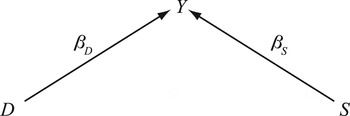
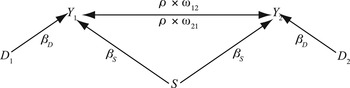
The simplest relationship between domestic and systemic variables is independence. Older IR research often focused on the effects of domestic variables independently from any effects of systemic influences, a theoretical relationship graphically depicted in Figure 1. These relationships link domestic variables, D, with outcomes of interest, Y, and do not ascribe any role to systemic variables. β D then describes the relationship between domestic factors and the outcome of interest. Much of the literature on endogenous protection in the trade area treated domestic factors as independent influences on trade policy.Footnote 31
Independence model

Direct Systemic Effects
Many theories imply a direct role for systemic influences, as well as domestic ones, on the outcome of interest, β S , as in Figure 2. For example, Li and Resnick's analysis explaining foreign direct investment (FDI) inflows into a country incorporates a systemic variable, the amount of world FDI inflows.Footnote 32 Still others incorporate systemic effects by using controls for unobserved systemwide heterogeneity—for example, year fixed effects.
Direct system effects

Indirect System Effects
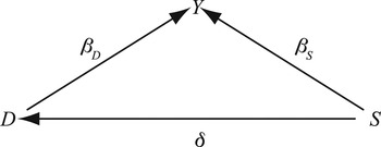
Other IR research has long considered indirect system effects, where systemic variables influence the value of domestic variables, which in turn, affect the outcome variable, as in Figure 3. Systemic variables can shape the outcome of interest directly (as in the previous category) via β S as well as indirectly via their influence on domestic variables, represented by δ. Gourevitch had this type of relationship in mind with his classic “second image reversed” analysis, in which the international system affected domestic politics, which then affected nations' foreign policy choices.Footnote 33
Indirect system effects

These types of relationships are often referred to as mediating relationships.Footnote 34 A domestic variable mediates the effect of a systemic variable if the systemic variable affects the value of the domestic variable. This generates two interesting effects to estimate: the direct effect of systemic variables on the outcome variable, β S , and the indirect effects of systemic variables through their effect on domestic variables, δ.
Moderation
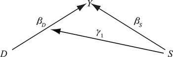
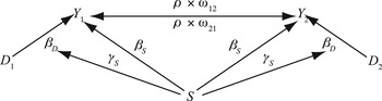
As the international environment has become complex with growing interactions among states and globalization, scholars have turned to more complicated models. One more complex interaction entails the moderating role of systemic variables. “Conceptually, a moderator is a variable that modifies the effect of a predictor on a response.”Footnote 35 According to Baron and Kenny, “moderator variables specify when certain effects will hold... [They] partition a focal independent variable into subgroups that establish its domains of maximal effectiveness in regard to a given dependent variable.”Footnote 36 As depicted in Figure 4, systemic variables alter how domestic variables affect the outcome of interest; γ1 describes how the effect of D on Y (β D ) is moderated by S. The figure depicts a relationship in which systemic variables moderate the effects of domestic variables, but we could also imagine that domestic factors might moderate the effects of systemic variables.
Moderating effect of systemic variable

Ahlquist and Wibbels, for instance, examine how international pressures can moderate domestic factors to explain democratic transitions.Footnote 37 World trade openness (a systemic variable) affects how a country's relative labor endowment shapes labor's preferences (domestic variables) and thus affects the probability of democracy (outcome variable).
Empirical models often examined moderating relationships using multiplicative interaction terms. Although it is less prevalent in IR, multilevel or hierarchical modeling is a powerful tool for analyzing such relationships. Multilevel modeling takes advantage of the researcher's knowledge that individual observations in the data are part of larger groups.Footnote 38 A classic example considers data on students in school systems. The students are grouped into classes; classes are grouped into schools; schools are grouped into districts, etc. Multilevel modeling describes this structure and describes individual and group-level similarities and differences.
IR scholars often consider data with a similar structure. Particular countries could be grouped regionally or temporally. For our application, it is natural to think about groupings based on the international system over time. Countries in the same time period share the common features of the system at that time, and observations in different time periods belong to different groups because they exist in different international contexts. Multilevel modeling affords the researcher the flexibility to model relationships where, for example, systemic factors change the way that domestic factors affect outcomes. If the theory proposes a hierarchical relationship where systemic factors describe the context in which domestic factors operate, the accompanying empirical model can directly capture these features. Model 1 is a statistical representation of a moderation relationship like that in Figure 4, where the systemic variable changes the relationship between the domestic and outcome variables.
 $$\eqalign{ Y_{it} & = \beta _0 + \; \beta _{0t} + \; \alpha _i + \; \beta _{D\comma t} D_{it} + \; \varepsilon _{it} \, \, \, \lpar \hbox{individual/micro-level model}\rpar \cr \beta _{0t} & = \; \beta _S S_t \; + \; c_t \, \, \, \lpar \hbox{system/macro-level model}\rpar \cr \beta _{D\comma t} & = \gamma _0 + \; \gamma _t S_t + \zeta _t \, \, \, \lpar \hbox{individual/micro-level model}\rpar }$$
The individual level of Model 1 describes relationships between country-level explanatory variables for a particular time period and the outcome of interest. At this level, both the outcome variable, Y it , and the explanatory variables D it vary across countries and time, and values of these variables are often measured at the country-year level. β0 is the global intercept for all observations. β0t is the year-specific intercept that captures the overall direct effect of the international system. α i is the country-specific intercept, which is equivalent to the familiar country fixed effects. The domestic source of Y it 's variation is from α i + β Dt D it , including the observed time-varying domestic factors D it and the unobserved, time-invariant country-specific characteristics included in α i . In the first system-level equation, the overall effect of the international system on the outcome, β0t , is further explained by the direct effect of the observed systemic variables, S t , and the unobserved ones left in the error term, c t .
More importantly, Model 1 captures moderation by allowing the effect of D to vary with changes in the system over time. As in the second system-level equation, the variation of D's effect is partially explained by the systemic variable S. The unexplained part of the over-time change of β D,t is left in the error term of the third line, ζ t . Plugging the system-level equations in the individual-level equation, we have the reduced model as follows:
 $$Y_{it} = \beta _0 + \; \gamma _0 D_{it} + \; \beta _S S_t + \; \gamma _1 D_{it} S_t + \; \alpha _i + c_t + u_{it}$$
where u it = ζ t D it + ε it .
This representation highlights a restricting assumption of the multiplicative interaction model (MIM) and an advantage of multilevel modeling (MLM). The two models are equivalent only if we assume there is deterministic moderation, that is ζ t = 0. In other words, the MIM assumes that the change in the effect of the domestic variable is a deterministic function of the moderator (that is, the systemic variable), β D = f(S t ) = γ0 + γ1 S t . But if there is an omitted systemic variable (the error term ζ is a stochastic term instead of the constant number 0), then the model invites the problem of inconsistency, and all coefficients, not only γ0 and γ1, could be affected.Footnote 39
If the researcher is confident that there are no omitted systemic moderators, the MIM is a legitimate choice for modeling the moderating effect of the systemic factor, S t , on the relationship between the domestic variable and the outcome variable. However, if we suspect that not all moderators are observed, then we have to address the relationship β D,t = γ0 + γ1 S t + ζ t and treat ζ t as a stochastic term (an error term), in which unobserved moderators are left out. The advantage of MLM lies in the fact that ζ t is not required to be independent of any of the observed covariates at any levels, because ζ t is treated as a parameter and can be estimated using maximum likelihood techniques or simulation methods. The MIM can be regarded as a special case of the multilevel model with an additional (and potentially strong) restriction ζ t = 0, that is, that there are no omitted moderators and no unobserved shocks to the moderation relationship.
Interdependence
Our final category considers interdependence, which models how units within the international system interact with one another. Such relationships are depicted in Figure 5 and are often the focus of the existing literature that utilizes network theory and spatial econometrics. Both are concerned with the possibility that the outcome in one unit, Y i , affects the outcome in another unit, Y j .
Interdependence

Spatial econometrics has become an often-used tool, particularly in the study of the diffusion of national policies across countries. Spatial econometrics explicitly incorporates the notion that one country's outcome variable can be influenced by spatially and/or temporally lagged outcome variables from other countries. It is hard not to encounter analyses using these tools in virtually every context.Footnote 40 The econometric tools themselves continue to be refined by social scientists studying IR and comparative politics.Footnote 41
These types of relationships can be estimated using Model 3 and its matrix equivalent, Model 4 as follows:
 $$Y_{it} = \; \rho _t W_{it} {\bi Y}_{\bi t} + \; \beta _D D_{it} + \; \beta _S S_t + \; \alpha _i + c_t + \; \varepsilon _{it}$$
The matrix expression of the model is as follows:
 $${\bi Y}_{\bi t} = \; \rho _t W_t {\bi Y}_{\bi t} + \; \beta _D {\bi D}_{\bi t} + \; \beta _S S_t + \; {\bi \alpha } + {\bi c} + {\rm \epsilon }_{\bi t}$$
where Y t = {Y it , … Y nt }, α t = {α i , … α t } and c t = {c t , … c t }. W is an n × n weighting matrix or metric, where each entry describes a measurement of the connectivity between any two units. The entry in cell w ij measures how connected the researcher expects units i and j to be, and the diagonal elements of the matrix are all 0.
Several features of the weight matrix W are worth highlighting. First, it is a matrix of measurements chosen by the researcher, using prior theoretical information. The spatial econometric techniques described in this article treat elements of this matrix as exogenous.Footnote 42 The researcher chooses some proxy, for example, distance, amount of bilateral trade, mutual organization membership, etc., that the researcher thinks describes the degree of connectivity between the units. The W matrix can also be time-varying, accounting for the possibility that particular units, i and j, are expected to be more or less intensely connected at different times, for example, if cell (i, j) of W measured the amount of bilateral trade between countries i and j. Conventionally, the matrix W is row-standardized for computational reasons.Footnote 43
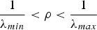
The parameter ρ t describes the strength and direction of contagion by the channels prespecified by W. Whereas W t is the observed data structure, ρ is an estimated parameter. When all the elements in W t are nonnegative, positive values of ρ imply that the outcomes for the units move in the same direction in general, and vice versa.Footnote 44 Higher absolute values of ρ denote stronger contagion across the units.Footnote 45
Because there are endogenous variables on both sides of Equation 4, this model is a simultaneous equation in the sense that all the outcomes in the same time period are determined simultaneously in the model. Therefore, denoting A = I − ρ t W t where I is the identity matrix, the model can be written as follows:
 $$\eqalign{ {\bi A\; }Y_t & = \beta _D {\bi D}_t+\; \beta _S \; S_t+{\bi a}+c_t+\epsilon _t \cr {\bi Y}_{\bi t} & = {\bi A}^{ - 1} \beta _D {\bi D}_{\bi t}+\; {\bi A}^{ - 1} \beta _S \; S_t+{\bi A}^{ - 1} {\bi a}+{\bi A}^{ - 1} c_t+{\bi A}^{ - 1} {\rm \epsilon }_t}$$
The matrix form of the spatial model shows why we get inconsistent estimates if we omit interdependence. If ρ t ≠ 0 and A ≠ I , then the error term A −1 ε t violates the i.i.d. assumption. More importantly, because A −1 appears everywhere on the right-hand side, including the error term and the covariate terms, there is an endogeneity problem affecting all parameters.Footnote 46
An important advance in the model we specified is that the spatial autoregressive coefficient ρ is allowed to vary across time. Existing spatial models assume that the direction and magnitude of contagion is constant over time. However, there are compelling reasons to believe that interdependence among states might increase or decrease over time, or be positive at some times and negative at others. For instance, Neumayer and Plümper argue that competition among capital-importing countries affects which capital-exporting countries they choose as partners for bilateral investment treaties (BITs).Footnote 47 A capital importer is more likely to sign a BIT with a capital exporter if other capital importers have also signed a BIT with that particular capital exporter. Implicitly, they assume that this competition is equally fierce over time. But we could imagine competition being more fierce when the capital available from capital exporters is scarce than when it is relatively abundant. Gleditsch and Ward conduct an analysis of whether democratic transitions spillover to neighboring countries from 1951–98.Footnote 48 Given the large geopolitical changes that occurred, for example, the end of the Cold War, it is likely that the intensity of this contagion varied over time. During the Cold War, fear of communist dominoes or hopes for regional outbreaks of democracy abounded, while democracy promotion in the post–Cold War era was often targeted at specific countries.
Similar stories are feasible in virtually every scenario where researchers have theoretical reasons to suspect interdependence or contagion across units. Interdependence as a result of international bargaining may become more intense as more countries join a particular international institution. As an institution gains members and increases in its prominence, countries might increasingly use it as a bargaining forum, making the members' choices increasingly interdependent. Diffusion processes, such as learning, might be more intense over time as improvements in information technology make it easier for political actors to gather precise information about one another's policies and their effects. If the degree of interdependence across units changes over time, this reflects important changes in the international system that researchers might be interested in.Footnote 49
MLM and Interdependence
Additionally, researchers can develop even more complex models by considering combinations of the categories of interactions described earlier, as Figure 6 depicts. Researchers can develop and test theories in which virtually any combination of relationships between systemic, domestic, and outcome variables is present.
Combination of direct, moderating effects, and interdependence

To further expand the frontier of possible models for complex systemic-domestic interactions, we could estimate a model that includes all of these potential relationships, as in Model 5:
 $$\eqalign{Y_{it} & =\; \beta _0 + \beta _{0t}+ \beta _{0i}+\; \rho _t W_{it} {\bi Y}_t+\; \beta _{Dt} D_{it}+\; \varepsilon _{it} \cr \beta_{0t} & = \beta _S S_t+c_t \cr \beta _{Dt} & = \gamma _0 + \gamma _S S_t + \zeta _t }$$
Model 5 incorporates direct systemic effects on the outcome of interest, allows unobserved and observed systemic variation to moderate the effects of domestic variables, and estimates spatial correlation with time-varying connectivity. Model 3 and Model 5 are more complex than ordinary multilevel models or standard spatial models, so in the applications we estimate them with a Bayesian approach using Markov Chain Monte Carlo simulation techniquesFootnote 50 —stochastic simulation techniques to make inferences based on the simulated distributions of the parameters given the observed data.Footnote 51 It is especially powerful for estimating complex and parameter-rich models. Using a Markov Chain Monte Carlo approach requires us to specify prior distributions of the parameters. Priors can incorporate any information the researcher has before the data are observed. We use uninformative priors to the parameters because we want the inferences to be mainly based on the data. From a Bayesian perspective, all assumptions can be regarded as priors. Different from priors of the unknown parameters, the prespecified weight matrix W can be interpreted as a prior on W with no uncertainty.
Application: Regime Type and Trade Policy
Having described a set of theoretical relationships and accompanying empirical models for systemic, domestic, and outcome variables, we now apply them to the relationship between trade policy and regime type. Trade policy and democratization in LDCs are the focus of Milner and Kubota. As unskilled labor-rich developing countries become more democratic, Milner and Kubota (MK) hypothesize they are less likely to turn toward protectionist tariffs to garner political support. MK analyze data on the outcome variable, tariff rates, for approximately 101 LDCs for the years 1970–99. Their central explanatory variable is domestic, measuring the regime type of country i in year t. They also collect data on a set of covariates, both domestic and systemic. Using a series of models, they find that democracy is negatively related to tariff rates.Footnote 52
Oatley criticizes MK's analysis for its omission of the moderating effect of systemic variables. He argues in favor of a macro theory that accounts for possible bargaining among countries in the World Trade Organization (WTO) forum. To link this theory with the empirical evidence, he argues for a conditional hypothesis and reestimates certain models from MK with a multiplicative interaction term between a dummy variable indicating a country's membership in the WTO and the regime type variable. He finds that democracy decreases tariffs only for WTO members and concludes that this is evidence of the biased inferences drawn from MK's analysis. Although a country's membership in the WTO is not a systemic variable, he argues that this shows the importance of systemic factors such as the WTO. Because MK did not consider a possible moderating role of systemic variables, Oatley claims that their conclusions were incorrect.Footnote 53
This section shows how a researcher might start with a simple relationship and walk through a series of increasingly more complicated models. Moving through the progression shows whether, or if at all, these assumptions affect the relationship of interest. In a sense, the simpler models make assumptions about the absence of features in the more complicated models
Data Set
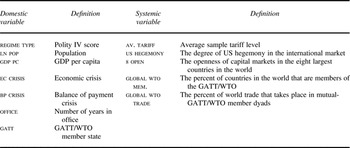
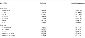
The data we use are identical to that of MK and Oatley's analyses, with a few exceptions. First, we significantly extend the period covered by either analysis. The original analyses covered the years 1970–99, which unfortunately include only four years of the post-WTO period. We extend the analysis to 2008, which triples the number of WTO-period years under consideration. Because we are concerned with modeling approaches, not variable selection, we focus on a consistent set of twelve explanatory variables. Table 1 lists the seven domestic and five systemic variables. The resulting data set covers thirty-nine years for eighty-five countries. We use multiple imputation to fill in the missing data to more efficiently use our information.Footnote 54
Domestic and systemic variables

We focus on one particular domestic variable, a country's regime type, which is measured with the standard combined Polity IV scores. We also include domestic control variables measuring the natural log of a country's population, ln pop, and its per capita gross domestic product, gdp pc. We include a dummy variable that equals 1 in years when a country experienced an economic crisis, for example, a severe inflation or negative income shock, or a balance of payment crisis, ec/bp crisis. We include a control for the number of years that the current government has been in office, office. We then include a dummy variable indicating membership in the GATT or WTO, gatt.Footnote 55
We also focus on five systemic variables. Three are from the original MK analysis. We measure the percent of world trade accounted for by US imports and exports to capture the degree of US hegemony in the international market, us hegemony. We also measure the openness of capital markets in the eight largest countries in the world, 8 open.Footnote 56 For country i in year t, we calculate the average tariff level for countries other than country i, av. tariff.Footnote 57 Lastly, we include systemic variables that measure the degree of WTO influence in the system. Unlike a country's GATT/WTO membership, which Oatley emphasizes, these two variables are systemic, not domestic. We measure the percentage of countries in the world that are members of the GATT/WTO in that year, global wto mem.Footnote 58 We also measure the percentage of world trade that takes place between mutual-GATT/WTO member dyads in a given year, global wto trade.Footnote 59 These systemic variables capture variation in the overall importance of the WTO to world trade. These variables are not binary, which allows us to consider richer variation.
“Baseline” Models
Before estimating multilevel and spatial models, we establish a set of baseline empirical results for the relationship between regime type and tariffs. These models are similar to the original approach in MK.Footnote 60 These empirical results reflect a theoretical relationship where domestic and systemic factors are separate variables that influence the outcome, such as those described earlier.
 $$Y_{it} = \beta _0 + \beta _D D_{it} + \beta _S S_t + \alpha _i + \varepsilon _{it}$$
 $$\hskip -9ptY_{it} = \beta _0 + \beta _D D_{it} + \alpha _i + \delta _t + \varepsilon _{it}$$
Models 6 and 7 are two variations of the familiar fixed effects models. Model 6 allows for domestic and systemic variables to have direct effects on the outcome of interest, and accounts for unobserved unit-level heterogeneity, as captured by α i , the unit-fixed effect. Model 7 allows for domestic variables to directly affect the outcome of interest, but also treats all systemic variation as unobserved, as captured by δ t , the year fixed effects.
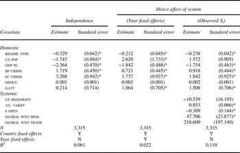
Table 2, columns 5 and 6, show the results from estimating the equation in Model 6. The coefficient on regime type is −0.238, suggesting that increased levels of democracy are associated with decreased tariffs. Table 2, columns 3 and 4 show the results from estimating the equation in Model 7. The results are very similar to results from Model 6, with a coefficient on regime type of −0.212. The first two columns in Table 2 show results from the simplest model assuming no systemic effects at all. The estimates based on the first model are notably different in the magnitude and direction from the two other models considering systemic effects, which suggests that it is incorrect to assume no systemic effects.
Independence and direct effects

Note: * Significant at 95% level.
Moderation
In the context of our trade policy data, we can imagine, theoretically, why moderating relationships might be present. For instance, the extent of global WTO membership might moderate the effect of regime type. If WTO members use these organizations as fora in which they collectively bargain over mutual tariff reductions, then we might expect the effect of regime type to be strongest when more countries are members of the WTO. When fewer countries are members, the effect of regime type might be dampened.
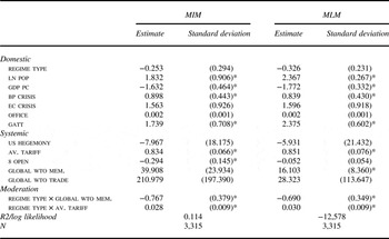
We demonstrate and compare the MIM and MLM approach to examine whether two systemic variables, global wto mem. and av. tariff, influence the relationship between regime type and trade policy. The results are in Table 3. The first two columns show the results from the MIM, and columns 3 and 4 are the estimates and standard errors from the MLM.
Moderation models: MIM and MLM

Note: * Significant at 95% level.
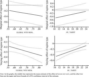
The results for regime type are easiest to interpret graphically in terms of the substantive effect of regime type on tariffs. Figure 7 shows how regime type affects tariffs from the MIM and MLM models. The top two panes correspond to results from the MIM, and the bottom two correspond to results from the MLM. For each (MIM and MLM), the left pane shows how the effect of regime type on trade openness varies with global wto mem., holding av. tariff constant at its sample mean. The right panes show how the level of av. tariff moderates the relationship between regime type and trade openness, holding global wto mem. constant at its sample mean. Both the MIM and MLM show that increased WTO membership magnifies the negative effect of regime type, whereas higher global average tariffs have the opposite effect.
Varying-effect of regime type moderated by global wto mem. and av. tariff

Although the MIM and MLM yield similar substantive results, the error bounds of the effect of regime type in MIM are systemically larger than those in MLM. This is expected because the MLM takes into account unobserved moderators whereas the MIM assumes that the observed moderators explain all the variation of the effect of regime type. Because the lower graphs are about
 ${\open E}\lpar \beta _{regime} \; \vert moderator\rpar $
, the error bounds are much smaller than their upper-panel counterparts. Although the MIM does not suggest the effect of regime type is significant except when 75 percent or more countries around the world are WTO members, the MLM suggests that regime type does have a significant negative effect on tariffs with various values of the two observed moderators.
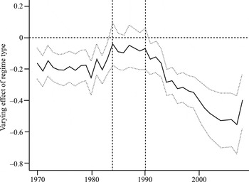
Figure 8 shows the overall effect of regime type on tariff levels in each particular year, taking into account both of our moderating systemic variables.Footnote 61 regime type has a consistently negative effect on tariff levels, though this effect is insignificant for a few years in the late 1980s. The overall effect of regime type, when accounting for moderation from these two systemic variables, is strongest in later time periods, especially after the early 1990s. The timing of this effect is unlikely to be accidental: the GATT regime officially transitioned to the WTO regime in January of 1994. Because the WTO regime is thought to be stronger in many ways than its predecessor, it is possible that the new regime magnified the tariff-dampening effects of regime type.
System-specific/time-specific effect of regime

As for other explanatory variables, most of the results of the MLM are similar to those based on the MIM, but there are some differences. For example, 8 open is important in the MIM but not significant in the MLM. And although gatt is significant in both models, the magnitude of the estimate is much larger in the multilevel model than in the interaction term model.
Interdependence
Theoretically, a researcher might be interested in whether mutual WTO membership helps countries negotiate reciprocal tariff reductions. Tariffs could therefore be positively correlated across units: if one WTO member lowered its tariffs, then another WTO member might be more inclined to do the same as they bargain over mutual or reciprocal reductions. In Oatley's criticism of Milner and Kubota, he argues that the WTO “provides a forum in which each government can exchange domestic tariff reductions for foreign tariff reductions.”Footnote 62 This is exactly the type of relationship that models described in the interdependence section capture.
To test these predictions and capture the “macro-theory” proposed by Oatley, we code a time-varying weighting matrix that indicates whether two countries are both WTO members. We construct W t where entry ≤ft (ij ) for the year t equals 1 if countries i and j are both members of the WTO in year t and is 0 otherwise. W t varies over time, since countries may join the GATT/WTO regime in different years in our sample. This matrix captures one specific interdependence mechanism—bargaining among WTO members—similar to the “macro theory” that Oatley proposed.
If bargaining processes are at work, and countries' tariff levels affect one another when both countries are WTO members, then we should expect ρ to be positive and significant. A positive ρ means that tariff levels are positively correlated across WTO members: when one WTO member lowers their tariffs, other WTO members tend to lower theirs. A negative ρ would suggest negative correlation across WTO members: when one WTO member lowers their tariffs, other WTO members tend to raise theirs. Because our model allows us to estimate ρ for each year, we can describe the degree to which tariffs are correlated across WTO members over time, and whether this correlation is positive or negative.
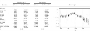
Table 4 reports the results.Footnote 63 For comparison, the first two columns show the results from a model in which ρ is not time-varying, and the second two columns show results from the time-varying ρ model.Footnote 64
Spatial modeling: Constant ρ and time-varying ρ

Note: * Significant at 95% level.
Moderation and interdependence: Time-varying W and ρ

Note: * Significant at 95% level.
The negative relationship between regime type and tariffs obtains even when accounting for possible interdependence among LDCs. In both versions of the interdependence model, the estimated coefficient for regime type is negative and significant, suggesting that the original results for regime type are robust to models including spatial correlation. Our results for some systemic variables, however, do change. After interdependence is incorporated, av. tariff is no longer significant, but global wto mem. still has a direct effect on tariff.
In addition to further examining the relationship between regime type and tariffs, these models provide information about the nature of interdependence of tariffs among LDCs. The last row in Table 4 reports the mean and standard error for the ρ term in the time-invariant ρ model, which is positive 0.949 and significant. This seemingly suggests that tariff levels are positively correlated across units—as one country raises or lowers its tariffs, its fellow WTO members tend to do the same. However, the standard error of ρ is as small as 0.043, which raises concerns about a unit root.Footnote 65
Returning to the time-varying ρ model, the graph in Table 4 shows that ρ has a distinct temporal trend.Footnote 66 For early years, ρ is largely indistinguishable from 0, with tariffs not strongly correlated through mutual GATT membership. In the middle years, ρ is positive and significant, as predicted. In later years, and contrary to the findings from the time-invariant ρ model, ρ is strongly negative and significant, meaning that mutual WTO membership actually made members' tariff levels inversely correlated.Footnote 67
The time-invariant model generated an optimistic result regarding WTO membership: dyads where both parties were members tended to lower their tariffs in tandem. The time-varying model generated a very different result. In the 1980s, the GATT appears to have had this effect. Yet for other periods of time, WTO membership appears not to have had this effect, or even had the opposite effect.
A negative value for ρ in this context is puzzling, and suggests the need for improvements in our theoretical arguments for how WTO membership affects members' tariffs directly and through contagion across members. This result could arise from the order in which countries joined the WTO. We might expect interdependence in the earlier and middle years to yield more positive diffusion effects, ρ's, as countries most willing and able to benefit from GATT membership joined and negotiated tariff reductions. The late-joining countries could be holdouts with the strongest political pressures to maintain higher tariffs. Because countries historically have not left the WTO, the membership in later years has been composed more of protectionist holdouts and preexisting members who have already negotiated lower tariffs. However, Allee and Scalera argue that most of the so-called automatic accessions, where countries joined the GATT quickly without making meaningful tariff concessions, occurred during earlier time periods (1960–67) with decolonization.Footnote 68 Additionally, many countries used this process in the early 1990s, right before this option was taken away by the new WTO regime. Many rigorous accessions, where joiners made substantial tariff cuts as a prerequisite to joining, took place during 1980s. Although other important rigorous accessions took place during the WTO era (for example, China), changing accession patterns could explain shifting patterns of interdependence among members' tariff levels. The results from the two models demonstrate that the nature of interdependence can change in substantively important ways that are uncovered only when allowing the degree of interdependence, that is, ρ, to vary over time.
Combining MLM and Interdependence
What if both moderation and interdependence are present, as in Figure 6? For illustration with our trade policy data, we estimate the following model:
 $$\eqalign{Y_{it} & = \beta _0 + \beta _{0t} + \beta _{0i} + \rho _t W_{it} {\bi Y}_{\bi t} + \; \beta _{Dt} D_{it} + \varepsilon _{it} \cr \beta _{0t} & =\; \beta _S S_t+c_t \cr \beta _{Dt} & = \gamma _0 + \zeta _t }$$
We do not have a theory suggesting that the observed four systemic variables would change the mechanisms through which the domestic variables affect trade openness, but there may be unobserved systemic variables that exert such moderating effects. The third line of the model reflects our consideration of moderation effects. Model 8 incorporates direct systemic effects (in the second line), allows unobserved system variation to moderate the effects of domestic variables (in the third line), and estimates spatial correlations with time-varying connectivity (in the spatial lag term in the first line).Footnote 69
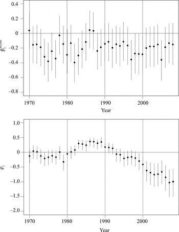
In general, the results are similar to those above. regime type has a negative and significant effect. The left pane of Figure 9 shows the estimated coefficient for regime type by year, accounting for unobserved systemic shocks. In almost all years, the coefficient is negative, and often significant, similar to the moderation results in Figure 7. The right pane shows the estimated interdependence or ρ over time, and the trend is again similar to the results from the figure in Table 4.
Time-varying effect of regime type and ρt

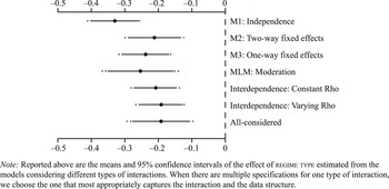
Given that we have presented a range of models intended to capture different possible domestic and systemic relationships, it is helpful to compare the similarities and differences across models with regard to how regime type affects tariffs. Figure 10 shows the interesting consistencies and differences between models. The simplest to most complicated models provide consistent answers about how regime type affects trade liberalization: democracy is positively and significantly associated with more liberalization. However, the effect of regime type differs in potentially meaningful ways across the models. In some models, the coefficient on regime type is as large as −0.329, and in others as small as −0.191. The simplest and most complicated models provide consistent answers to the question about regime type's effect on trade liberalization: more democracy is positively and significantly associated with more liberalization. Using simple empirical models does not necessarily distort results. It can provide a baseline to evaluate the robustness of domestic politics' impact on outcomes before taking into account the more complex nature of linkages to the international system. In this case and perhaps others, simple models perform well. This may reflect the persistent fact that linkages and interactions within countries remain much denser than those across countries' borders.
Effect of regime type: Different types of interaction considered

Conclusion
One of the most important and enduring debates in IR and IPE concerns the relative weight of systemic versus domestic factors in explaining outcomes. A central issue in the older “isms” debate among realists and liberals revolved around whether domestic or systemic factors best explain international relations. In more recent IPE work, the main source of contention over the impact of globalization also relates to this issue: To what extent will global economic forces overwhelm domestic institutions in this new era? As a recent study about the global race to the bottom points out, “Defying zero-sum predictions, the race to the bottom does not signify the end of domestic politics, and national differences are far from extinct.”Footnote 70 This debate shows little sign of waning. Most scholars believe that both sets of factors are important, and that the interaction of domestic and international variables is the new normal. The big question is what this interaction looks like and how much weight each set of factors carries.
To help provide a map for this research, we have drawn from an array of literature to set forth five of the most common models of that interaction. Oatley concluded his challenge to IPE scholars by arguing in favor of “[embedding] distinct approaches within a common overarching framework.”Footnote 71 We take concrete steps toward that goal. If the theoretical argument being employed views systemic or domestic factors as one of many influences that determine outcomes, then the simpler models we present may suffice. If the theory focuses on the interplay between systemic and domestic factors and how they moderate one another, then multilevel models can help describe that hierarchy. If the theory prioritizes strategic interaction, interdependence, or contagion of outcomes across units, then the later spatial models are more appropriate. The most complex models incorporate all of these different forms of systemic influences.
The appropriate approach also depends on the researcher's theoretical knowledge about the microfoundational relationships among units in the system and what this implies for the role of the system. The first model, involving independence of units from system effects, does not seem particularly robust in our modern world. Such models are rare in the literature in CPE/IPE. The harder task is distinguishing whether to use one of the other earlier approaches involving direct, indirect, or moderating effects or the latter approaches involving interdependence. The difference between the two sets of approaches does not lie in whether they incorporate a system in some way. None of them considers units as isolated from one another in a completely decomposed system.
The difference instead lies in how each conceives of the system and its effects. The first set of models allows units to affect one another through exogenous interaction effects. The systemic channels through which agents can affect each other are not created through the endogenously modeled choices that agents make. The system posited therein affects the agents, but the agents' actions do not change the system within the scope of these models. For these less complex models (that is, direct, indirect, and moderating system effects), the influence of the system operates on the agents and does not feed back to the system level.
Such models are appropriate if the researcher thinks that units within a system are connected through mechanisms other than the outcome variables of interest. For example, countries could be connected with one another systemically and affected by exposure to common, exogenous shocks. Or the units could be affected by exposure to system-wide trends that affect the context in which the units make decisions.
The interdependence models consider the system to be a set of endogenous interaction effects. The system in the interdependence model is determined by the exogenous structure of dependence, the endogenous outcomes chosen by all the agents, and the endogenous interaction process (modeled by ρ). In the interdependence models, there is feedback. Agents affect the international system through their actions or choices, and the system in turn affects all agents. The system affects the agents by providing channels for complicated and iterative spillover effects between agents. These spillover effects can be “local”; one agent's action affects another agent through the channel specified by the weighting matrix. Spillover effects are also “global”; one agent affects another, which affects another, and so on, like ripples on a pond.Footnote 72 The interdependence model may be better understood as a simultaneous equation model to mutually constitute the system and agents. The unknown parameter ρ and the exogenous structure W are how the agents and the system interact as well as how the agents interact among themselves. The effects of the agents on the evolution of the system in the interdependence model derive from the fact that interactions of the agents change the level of connectivity of the system over time, thus altering the previous equilibrium state reached through complicated strategic interactions among the agents.
Hence one should choose the interdependence model when one believes that the system is evolving along with the agents, and the evolutions of the system and the agents are (at least partially) mutually determined by the actions of the units. This is most likely the case when the units or states are “large” in the sense that they have enough capability to shape the system and other states' beliefs or behavior. If the units are almost all “small,” that is, they lack the capabilities to affect the system and other states, then the first models we propose are more useful. As we show in our trade policy example, when looking at the developing countries it is not clear that they—or the vast majority of them—are “large” enough to affect the system. Perhaps that is why we are seeing small interdependence effects in this case.
In sum, using the interdependence model allows one to examine these more complex spillovers through mechanisms such as learning, diffusion, or competition. The agents in effect change themselves and one another by changing the system. In the previous models the agents do not change the system because it is exogenous. If the researcher thought that individual agents did not or could not have important effects on the overall system, then the earlier, less complex models may be appropriate.
Recent iterations of the agent-structure debate characterize existing research as falling into one of two extremes: either the research models networks and systemic connectedness between units or the research treats units as completely separate from one another. And because (as the argument goes) it is uncontroversial that units are connected in some way in today's globalized world, it follows that the latter type of research is indefensible, and that the conclusions drawn are likely to be biased so that researchers should deemphasize the search for law-like empirical regularities altogether.Footnote 73 Our road map shows that this argument is based on a false dichotomy. A researcher need not choose between assuming that everything (or nothing) is connected. There is a wide array of approaches that fall somewhere in between. What empirical model to choose depends on what type of relationship operates between the units, that is, on the microfoundations. If it is through exogenous systemic shocks or the overall context, then our first four models are more appropriate. If it is through endogenous actions or feedback, then the interdependence type of model is most appropriate.
Beyond describing where a researcher might start, the road map also provides guidance for where to end. Which model best explains an outcome is likely to vary with the issue at hand. Employing the most complex model of interaction is not necessarily the best path to take, especially as an initial step. It may be much more informative to start simply and then see if the addition of complex interactions changes the explanation substantially. In the case of the role of democracy in promoting trade liberalization in the developing countries in the past few decades, which we analyzed extensively in this article, it is not clear how much explanatory power is gained from using highly complex models of systemic-domestic interaction. Simpler models may capture the essence of the explanation well. Occam's razor and the principle of parsimony make us aware that simpler explanations may be preferable. When systems are nearly decomposable as Simon points out, starting from simpler models still makes a good deal of sense.
We also contribute to the development of more complex models by putting renewed attention on multilevel models and adding to diffusion studies. Multilevel models may be a preferable way of conceiving of systemic factors' impact. These models assume a natural hierarchy of effects: systemic pressures in effect cast a shadow over all domestic influences. This is but one way to conceive of the interaction of domestic and systemic factors, but it is a powerful and important one.Footnote 74
We also developed a model in which the nature of contagion and interdependence among units in the system can change over time. Adding an element of time to studies of how global processes diffuse is important. While diffusion may proceed over time in a uniform and unchanging way, it may also take on time-varying forms that are novel to study. Hence our two new modeling ideas add to the stock of complex models of systemic-domestic interaction that one can envision.
We view these contributions as complementary to other recent advances in which the system is conceived as the result of interdependence among the units caused by processes like international bargaining, diffusion, or competition. We have taken one particular approach, associated with spatial econometrics, that treats the nature of connections between units as exogenous and then models how outcomes across units affected one another. Other approaches treat behavior and outcomes of units as exogenous, and endogenously model or describe the nature of connections between units.Footnote 75 Some research has begun to focus on modeling both the behavior and connectivity of units, with the goal of describing the evolution of networks or feedback processes.Footnote 76 As this research progresses theoretically and empirically, it will enable future work to push even further beyond the categorizations and methodological advances we provide here.
Supplementary material
Replication files and empirical data for this article can be found at http://dx.doi.org/S0020818314000356.