1. Introduction
Transport and mixing inside a confined environment is of critical importance for many engineering processes. In particular, natural thermal convection is an efficient and non-intrusive way to induce unsteady motion inside a closed fluid container. Natural convection is therefore crucial for the spreading of pollutants or aerosols impurities in e.g. cooling devices, ventilation of building interiors or during the solidification of alloys. All transport mechanisms combine two different physical processes: advection and molecular diffusion. Advection acts on a timescale
 $t_{ad}\approx U/L$
while diffusion acts on a timescale
 $t_{d}\approx L^{2}/D$
, where
 $U$
and
 $L$
are characteristic velocity and length scales and
 $D$
is a typical diffusion coefficient. The case of non-diffusive mass transport corresponds to the limit
 $t_{d}/t_{ad}\rightarrow \infty$
, with advection the only possible mechanism responsible for mixing. Defining the kinematic viscosity
 ${\it\nu}$
of the fluid, a Schmidt number
 $\mathit{Sc}$
can be defined as
 $\mathit{Sc}={\it\nu}/D$
. The smallest relevant scale
 ${\it\eta}_{c}$
of the concentration field scales as
 $\mathit{Sc}^{-1/2}$
, thus in the non-diffusive limit
 ${\it\eta}_{c}\rightarrow 0$
. Therefore, in this limit the concentration field cannot be resolved using finite resolution. We will focus here on the advection of perfectly passive pointwise tracers advected by a fluid flow, neglecting molecular diffusion as well as drag, particle size effects and interaction between particles. Equivalently the tracers can be thought of as fluid particles whereas the fluid itself is seen as a continuum. Consequently, we turn our attention towards a Lagrangian description of the dynamics of individual tracers, see for instance Grigoriev & Schuster (Reference Grigoriev and Schuster2011) and Aref (Reference Aref2014) for recent reviews on Lagrangian advection.
We focus in this study on the mixing of tracers by a prototype of natural convection flow inside a closed cavity. In the presence of a non-zero temperature gradient between two opposite vertical walls, the fluid is always in motion and there is no conductive state. The fluid rises near the hot wall and sinks along the cold wall, resulting in a recirculating flow around the cavity. Under the Boussinesq hypothesis, the flow is incompressible and will be investigated here numerically in a two-dimensional geometry. The two-dimensional configuration has been investigated extensively in tall or wide cavities (e.g. Paolucci & Chenoweth Reference Paolucci and Chenoweth1989; Ravi, Henkes & Hoogendoorn Reference Ravi, Henkes and Hoogendoorn1994; Xin & Le Quéré Reference Xin and Le Quéré1995; Le Quéré & Behnia Reference Le Quéré and Behnia1998; Xin & Le Quéré Reference Xin and Le Quéré2006), using different fluids such as air or liquid metals (Mercader, Batiste & Ruiz Reference Mercader, Batiste and Ruiz2004; Mercader et al.
Reference Mercader, Batiste, Ramirez-Piscina, Ruiz, Rüdiger and Casademunt2005), and has been the subject of several numerical benchmarks. The first bifurcations towards unsteadiness, as the Rayleigh number
 $\mathit{Ra}$
increases, have been well studied in the literature (Burroughs et al.
Reference Burroughs, Romero, Lehoucq and Salinger2002). However, Lagrangian mixing in this prototype of closed convection has to the best of the authors’ knowledge not been addressed yet. Since no analytical solution is available for this closed flow, this represents an interesting opportunity to test classical advection tools developed in the context of kinematic models. In practice we use direct numerical simulation (DNS) to generate the flow field on a finite grid at every time.
Mixing is considered complete if any initial blob of particles has been homogeneously dispersed, after a sufficiently long time, through the whole fluid domain. The mixing property implies that the system is ergodic and that particle trajectories are chaotic (Falkovich Reference Falkovich and Scott2004). More intuitively, the chaotic nature of mixing can be seen as a succession of stretching and folding events (see Ottino Reference Ottino1990; Sturman, Ottino & Wiggins Reference Sturman, Ottino and Wiggins2006). The chaotic nature of the trajectories requires the associated dynamical system, if it is autonomous, to be at least three-dimensional. For two-dimensional trajectories, mixing requires the velocity field to be time-dependent. The onset of two-dimensional mixing is thus expected to occur after (or to coincide with) the onset of unsteadiness of the flow. The dynamical system picture of chaotic advection, based on the identification of invariant sets, has been pioneered by Aref (Reference Aref1984) and widely used in, e.g., Rom-Kedar, Leonard & Wiggins (Reference Rom-Kedar, Leonard and Wiggins1990), Ottino (Reference Ottino1990) and Wiggins & Ottino (Reference Wiggins and Ottino2004). The theory, in the case of unsteady two-dimensional flows, relies heavily on properties of non-integrable Hamiltonian systems, such as the presence of Kolmogorov–Arnold–Moser (KAM) tori acting as barriers against transport. The notion of invariant sets acting as material barriers has more recently been generalised to arbitrary unsteady flow fields via the concept of Lagrangian Coherent structures (see e.g. Peacock & Dabiri (Reference Peacock and Dabiri2010) and references therein). A complementary interpretation of mixing as an example of chaotic scattering, based on the concept of chaotic saddle, has been suggested in the case of open flows (Jung, Tél & Ziemniak Reference Jung, Tél and Ziemniak1993; Ziemniak, Jung & Tél Reference Ziemniak, Jung and Tél1994; Lai & Tél Reference Lai and Tél2011). It was shown that the scattering region responsible for the mixing of tracers is built around infinitely many (unstable) periodic trajectories.
Our main motivation is to characterise the emergence of mixing in the differentially heated cavity flow as the flow field becomes unsteady. The continuous evolution from partial to complete mixing is quantified using a box-counting procedure. More specifically, the oscillatory nature of the velocity field suggests the use of perturbative methods, such as Melnikov functions and resonance criteria. This represents an opportunity to test these methods beyond their restrictive expected range of validity. In the first part, a scattering approach is used to distinguish between the different mixing regions of the flow according to their statistical properties. The second part aims at identifying the invariant sets of the system, assigning to each of them a specific role in the mixing process. Identification of invariant sets is based on the extraction of many (unstable) periodic orbits, along with their stable and unstable manifolds. The role of homoclinic and heteroclinic orbits, as well as that of toroidal trajectories, is specified in connection with the statistics deduced from the scattering approach. In the third part, we focus on one value of the control parameter
 $\mathit{Ra}$
for which the time-periodic regime is closest to achieving complete mixing. In such a regime a quasi-homogeneous distribution of tracers can be obtained asymptotically by seeding the tracers initially from one single location. The homogenisation process is examined and described as a succession of several steps, the latter of which allows for an estimation of the rate of homogenisation (also called mixing rate).
The paper is organised as follows. In § 2, we briefly recall the main results of previous studies of two-dimensional differentially heated cavities and describe the tools used for the numerical simulation of the cavity flow. The Lagrangian formulation of the problem is introduced in § 3, where we extend the scattering approach to this closed system in order to highlight the regions of the flow most relevant for mixing. Section 4 is dedicated to the identification of the most important invariant sets in association with their mixing properties. Section 5 suggests a quantification of the fraction of chaos in the system versus
 $\mathit{Ra}$
. It suggests that the upper end of the oscillatory regime corresponds to almost complete mixing. We focus in § 6 on the mixing induced by a localised source of tracers and verify the previous suggestion. The results and perspectives are eventually discussed in the concluding § 7.
2. Eulerian approach
2.1. Description of the flow
A two-dimensional differentially heated cavity is a closed container whose two vertical walls are subject to different homogeneous temperatures. The temperature of the hot and cold walls are denoted by
 ${\it\theta}_{h}$
and
 ${\it\theta}_{c}$
, respectively (see figure 1). We refer to
 $x$
and
 $z$
as the horizontal and vertical directions, respectively. The origin of the system
 $(x,z)=(0,0)$
is set as the bottom left corner of the cavity. The gravity
 $g$
is parallel to the heated walls and points downwards in the
 $z$
direction. This system is characterised by its height
 $H$
and width
 $W$
, and the aspect ratio of the cavity is defined as
 $A=H/W$
. The difference in temperature between the hot and the cold wall is defined as
 ${\rm\Delta}{\it\theta}={\it\theta}_{h}-{\it\theta}_{c}$
.
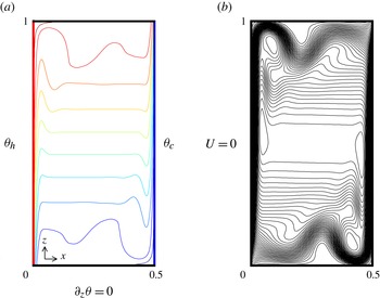
The differentially heated cavity with geometrical aspect ratio
 $A=2$
for the steady state at
 $\mathit{Ra}=10^{8}$
: (a) isovalues of the temperature field
 ${\it\theta}$
from hot (top, red online) to cold (bottom, blue online); (b) streamlines. Boundary conditions for the velocity are
 $\boldsymbol{U}=0$
at each walls. Gravity points downwards in the
 $z$
direction.

Following the classical Boussinesq hypothesis, we assume that the thermophysical coefficients of the fluid are constant except for the density in the buoyancy force, which expands as
 $$\begin{eqnarray}{\it\rho}({\it\theta})={\it\rho}_{0}[1-{\it\beta}({\it\theta}-{\it\theta}_{0})],\end{eqnarray}$$
where
 ${\it\theta}_{0}=({\it\theta}_{h}+{\it\theta}_{c})/2$
and
 ${\it\rho}_{0}=\text{const}$
. Defining
 ${\it\kappa}$
as the thermal diffusivity of the fluid,
 ${\it\nu}$
as the kinematic viscosity and
 ${\it\beta}$
as the thermal expansion coefficient, a Rayleigh number based on the cavity height is defined as
 $$\begin{eqnarray}\mathit{Ra}=\frac{g{\it\beta}{\rm\Delta}{\it\theta}H^{3}}{{\it\nu}{\it\kappa}},\end{eqnarray}$$
and the Prandtl number as
 $\mathit{Pr}={\it\nu}/{\it\kappa}$
.
Following the nomenclature of Xin & Le Quéré (Reference Xin and Le Quéré2006), the reference length is chosen as
 $H$
, the reference velocity as
 $V_{ref}={\it\kappa}\mathit{Ra}^{1/2}/H$
and the reference pressure as
 $P_{ref}={\it\rho}_{0}V_{ref}^{2}{\it\nu}/{\it\kappa}={\it\rho}_{0}g{\it\beta}{\rm\Delta}{\it\theta}H$
. The convective time unit is defined by
 $t_{conv}=L_{ref}/V_{ref}=H^{2}/({\it\kappa}\mathit{Ra}^{0.5})$
. We use a reduced dimensionless temperature
 ${\it\Theta}=({\it\theta}-{\it\theta}_{0})/{\rm\Delta}{\it\theta}$
. Using dimensionless variables
 $\boldsymbol{U}$
for the velocity field,
 $P$
for the pressure,
 ${\it\Theta}$
for the temperature,
 $X$
for the horizontal direction and
 $Z$
for the vertical direction, the Navier–Stokes equations read
 $$\begin{eqnarray}\displaystyle & \displaystyle \partial _{t}\boldsymbol{U}+(\boldsymbol{U}\boldsymbol{\cdot }\boldsymbol{{\rm\nabla}})\boldsymbol{U}=\mathit{Pr}(-\boldsymbol{{\rm\nabla}}P+\mathit{Ra}^{-1/2}{\rm\nabla}^{2}\boldsymbol{U})+{\it\Theta}\boldsymbol{e}_{\boldsymbol{z}}, & \displaystyle\end{eqnarray}$$
 $$\begin{eqnarray}\displaystyle & \displaystyle \partial _{t}{\it\Theta}+(\boldsymbol{U}\boldsymbol{\cdot }\boldsymbol{{\rm\nabla}}){\it\Theta}=\mathit{Ra}^{-1/2}{\rm\nabla}^{2}{\it\Theta}, & \displaystyle\end{eqnarray}$$
 $$\begin{eqnarray}\displaystyle & \displaystyle \boldsymbol{{\rm\nabla}}\boldsymbol{\cdot }\boldsymbol{U}=0. & \displaystyle\end{eqnarray}$$
Boundary conditions for the temperature are set as adiabatic for the two horizontal walls (Neumann conditions) and isothermal (Dirichlet conditions) for each vertical wall:
 $$\begin{eqnarray}\left.\begin{array}{@{}l@{}}{\it\Theta}(0,Z)=0.5=-{\it\Theta}(1/A,Z)\\ \partial _{Z}{\it\Theta}(X,0)=0=\partial _{Z}{\it\Theta}(X,1).\end{array}\right\}\end{eqnarray}$$
The velocity field obeys the no-slip condition
 $\boldsymbol{U}=0$
at all walls. The bounded fluid domain defined by the cavity is referred to as
 $\mathscr{D}=\{\boldsymbol{X}=(X,Z),X\in [0,A^{-1}],Z\in [0,1]\}$
. For this study we fix
 $\mathit{Pr}=0.71$
, which corresponds to air, and
 $A=2$
. The Rayleigh number
 $\mathit{Ra}$
is the only control parameter in our study.
2.2. Numerical method
DNS was performed using a code written by S. Xin and P. Le Quéré. It is based on a pseudo-spectral Chebyshev collocation method for the spatial discretisation and a direct Uzawa method for the velocity–pressure coupling. The time-stepping algorithm combines a second-order Adams–Bashforth extrapolation for the convective terms with a second-order backward differentiation formula for the linear ones. The resulting Helmholtz equations are solved by full diagonalisation of the second-order partial derivatives. Based on previous works, for all
 $\mathit{Ra}$
values presented in this paper, we used 81 and 101 collocation points in the
 $X$
and
 $Z$
directions, respectively, with a timestep of
 ${\rm\Delta}t=10^{-3}$
. This resolution is sufficient to accurately predict the first Hopf bifurcations of the system (Xin & Le Quéré Reference Xin and Le Quéré2006). Accurate convergence towards steady states below and beyond
 $\mathit{Ra}_{c}$
(where the steady state is unstable) is achieved using the selective frequency damping algorithm (Åkervik et al.
Reference Åkervik, Brandt, Henningson, Hœpffner, Marxen and Schlatter2006), with the convergence criterion
 $\Vert \boldsymbol{u}(t)-\boldsymbol{u}(t-{\rm\Delta}t)\Vert _{\infty }<10^{-10}$
and
 $\boldsymbol{u}=(U,W,{\it\Theta},P)$
.
2.3. Steady base flow
Due to buoyancy, fluid rises along the hot wall and sinks along the cold wall irrespectively of the value of
 $\mathit{Ra}$
. As
 $\mathit{Ra}$
increases, vertical boundary layers narrow while a homogeneous stratification appears in the core of the cavity for
 $\mathit{Ra}\gtrsim 10^{6}$
. At
 $\mathit{Ra}\approx 10^{7}$
detached recirculations form in the vicinity of two of the cavity corners. In addition, for all times the base flow
 $\boldsymbol{u}$
respects the
 $Z_{2}$
inversion symmetry
 $$\begin{eqnarray}\boldsymbol{u}(R\boldsymbol{X},t)={\it\zeta}\boldsymbol{u}(\boldsymbol{X},t),\end{eqnarray}$$
where the operators
 $R$
and
 ${\it\zeta}$
are defined by
 $$\begin{eqnarray}\left.\begin{array}{@{}l@{}}R\!:(X,Z)\rightarrow (1/A-X,1-Z),\quad R^{2}=I\\ {\it\zeta}\!:(U,W,{\it\Theta},P)\rightarrow (-U,-W,-{\it\Theta},P),\quad {\it\zeta}^{2}=I.\end{array}\right\}\end{eqnarray}$$
The base flow is shown in figure 1 for
 $\mathit{Ra}=10^{8}$
. The stratified core of the base flow supports internal gravity waves. The relaxation time of the least-damped internal waves varies as
 $0.1\times \mathit{Ra}^{1/2}$
, which is typically
 $10^{3}$
convective time units for
 $\mathit{Ra}\approx 10^{8}$
(Le Quéré & Behnia Reference Le Quéré and Behnia1998).
2.4. Onset of unsteadiness
The first Hopf bifurcation of the Eulerian system occurs at
 $\mathit{Ra}_{c}=1.5865\times 10^{8}$
(Xin & Le Quéré Reference Xin and Le Quéré2006). The bifurcated state exhibits oscillations of the two detached areas in phase opposition, together with an internal mode oscillating less vigorously in the core of the cavity. It is characterised by an angular frequency
 ${\it\omega}_{0}=2{\rm\pi}/T_{0}\simeq 0.28225$
, with the period
 $T_{0}$
only weakly varying with
 $\mathit{Ra}$
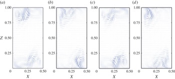
. Four different phases
 ${\it\Phi}=2{\rm\pi}t/T_{0_{[2{\rm\pi}]}}$
of the corresponding global mode are shown in figure 2 for
 $\mathit{Ra}=1.6\times 10^{8}$
. As reported in Burroughs et al. (Reference Burroughs, Romero, Lehoucq and Salinger2002), the corresponding solution
 $\boldsymbol{v}(\boldsymbol{X},t)$
of the linearised problem exhibits the anti-symmetry property
 $$\begin{eqnarray}\boldsymbol{v}(R\boldsymbol{X},t)={\it\zeta}\boldsymbol{v}(\boldsymbol{X},t+{\rm\pi}/{\it\omega}_{0})\end{eqnarray}$$
while the full nonlinear field does not (Le Quéré & Behnia Reference Le Quéré and Behnia1998). For
 $\mathit{Ra}\simeq 2.07\times 10^{8}$
, the time-periodic state along this branch undergoes a secondary Hopf bifurcation. The new bifurcated state is characterised by the additional propagation of rolls confined to the vertical boundary layers, with an angular frequency
 ${\it\omega}_{2}\simeq 3.0919$
. The resulting regime is quasiperiodic in time and will not be investigated here. We however report the value of
 $\mathit{Ra}$
at which it bifurcates since it marks the upper limit in
 $\mathit{Ra}$
of the time-periodic regime.
Departure from steady state of the velocity field for
 $\mathit{Ra}=1.6\times 10^{8}$
. The steady state has been obtained with the SFD algorithm: (a)
 $t=T_{0}$
; (b)
 $t=T_{0}+T_{0}/4$
; (c)
 $t=T_{0}+2T_{0}/4$
; (d)
 $t=T_{0}+3T_{0}/4$
.

3. Dynamics of tracers
3.1. Particle tracking: numerical method
Our Lagrangian approach is based on post-processing the velocity field obtained from the DNS computations. Whereas only one velocity field needs to be stored in the steady regime, in the oscillatory regime the period
 $T_{0}$
is split into approximatively
 $2\times 10^{4}$
snapshots. Usually,
 $T_{0}$
is a priori not an integer multiple of
 ${\rm\Delta}t$
, consequently, a fifth-order polynomial interpolation is performed to compute the last timestep of the period.
In the Lagrangian formulation, the motion of a non-diffusive tracer is described by
 $$\begin{eqnarray}\dot{\boldsymbol{X}}(t)=\boldsymbol{U}(\boldsymbol{X},t),\end{eqnarray}$$
where
 $\boldsymbol{U}$
is the solution of (2.3). Here
 $\boldsymbol{U}$
fields are extracted from DNS and fifth-order Chebyshev polynomial interpolation is used to determine the velocity field
 $\boldsymbol{U}$
at any arbitrary spatial location. Owing to the post-processing approach, spatial interpolation leads to faster computations than a Galerkin evaluation of the velocity field. The position of the particle
 $\boldsymbol{X}(t)$
is updated using a fourth-order Runge–Kutta scheme using as a timestep
 ${\rm\Delta}t=10^{-3}$
(identical to the timestep in the DNS). The accuracy of the scheme is assessed by quantifying the closure of streamlines in the steady regime for
 $\mathit{Ra}=2.05\times 10^{8}$
. While streamlines should be closed periodic trajectories, with our parameters the average closure error is in practice below
 $5\times 10^{-7}$
and around
 $10^{-4}$
for streamlines around saddle points.
3.2. Tracers in steady velocity fields
In an incompressible two-dimensional flow, (3.1) combined with the divergence-free condition (2.5) leads to
 $$\begin{eqnarray}\left\{\begin{array}{@{}l@{}}{\dot{X}}(t)=\partial _{Z}{\it\Psi}(X,Z,t)\\ {\dot{Z}}(t)=-\partial _{X}{\it\Psi}(X,Z,t)\end{array}\right.\end{eqnarray}$$
where
 ${\it\Psi}$
is the streamfunction. The system (3.2) has a Hamiltonian structure. When
 ${\it\Psi}={\it\Psi}_{0}(X,Z)$
is time-independent, the system (3.2) is integrable. In this case, the trajectories of the tracers coincide with the isocontours of
 ${\it\Psi}$
(i.e. streamlines) and chaotic advection does not occur.
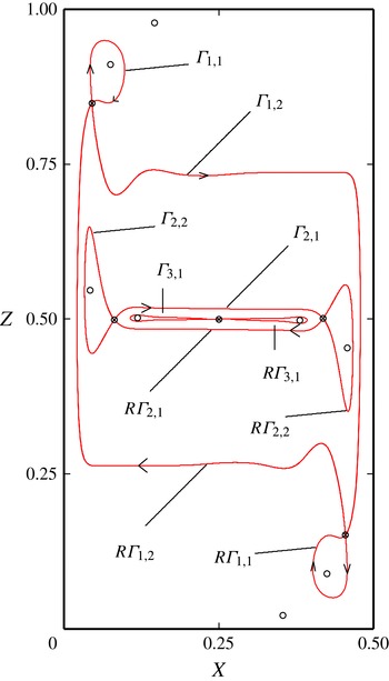
We first focus on the topology of the steady velocity field displayed in figure 3, which is organised around the fixed points of
 $\boldsymbol{U}$
. Streamlines originating from saddle fixed points of the velocity fields either form homoclinic loops, closing on the fixed point, or heteroclinic orbits connecting two different saddle fixed points together. Their period is infinite due to the slowing down in the vicinity of the fixed points. We identified in total five saddle fixed points (referred to as
 $\boldsymbol{X}_{S_{i}},\ i=1,\dots ,5$
) and four centres. (Fixed points of the steady velocity field were found using the algorithm described in the appendix A.) Owing to the centro-symmetry,
 $\boldsymbol{X}_{S_{4}}=R\boldsymbol{X}_{S_{1}}$
and
 $\boldsymbol{X}_{S_{5}}=R\boldsymbol{X}_{S_{2}}$
. The three saddle points
 $\boldsymbol{X}_{S_{1}}$
,
 $\boldsymbol{X}_{S_{2}}$
and
 $\boldsymbol{X}_{S_{3}}$
lie near the corner vortex, at mid-height of the cavity near the hot wall and at the geometrical centre of the cavity, respectively. They are associated with three homoclinic and two heteroclinic connections. Those connections are referred to as
 ${\it\Gamma}_{i,j}$
where
 $i=1,2,3$
is the label of the saddle point
 $\boldsymbol{X}_{S_{i}}$
and
 $j=1,2$
refers to the direction considered in each unstable eigenspace.
Homoclinic and heteroclinic connections of the (unstable) steady base flow for
 $\mathit{Ra}=1.625\times 10^{8}$
. Filled circles: saddle points; open circles: centres.

For any initial condition
 $\boldsymbol{X}_{0}$
belonging to a closed streamline, we can define the period
 $T_{SL}(\boldsymbol{X}_{0})$
of the corresponding orbit. A spatial distribution of
 $T_{SL}$
is obtained by seeding at
 $t=0$
the segment
 ${\bf\chi}=\{X_{0}\in ]0,1/(2A)],Z=A/2\}$
with
 $10^{5}$
tracers. Tracers are labelled by their initial horizontal position
 $X_{0}$
in
 ${\bf\chi}$
. For each of them, equation (3.1) is integrated up to time
 $T_{SL}$
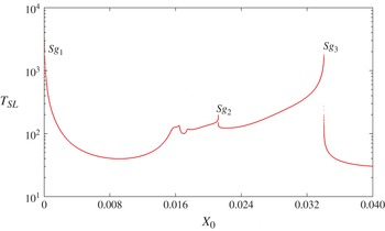
after which the tracer has come back to its initial position. The distribution of
 $T_{SL}$
versus
 $X_{0}$
is shown in figure 4 for
 $\mathit{Ra}=1.625\times 10^{8}$
. It is smooth except for the presence of three singularities of
 $T_{SL}$
(referred to as
 $\mathit{Sg}_{i}$
,
 $i=1,2,3$
). Here
 $\mathit{Sg}_{1}$
is related to the no-slip at the wall whereas
 $\mathit{Sg}_{2}$
and
 $\mathit{Sg}_{3}$
are the signatures of the heteroclinic and homoclinic connections
 $R{\it\Gamma}_{1,2}$
and
 ${\it\Gamma}_{2,2}$
, respectively. A last zone not displayed in figure 4 lies around
 $\boldsymbol{X}_{S_{5}}$
, the geometrical centre of the cavity, and is bounded by the heteroclinic connections
 ${\it\Gamma}_{2,1}$
and
 $R{\it\Gamma}_{2,1}$
. That zone features two homoclinic loops attached to
 $\boldsymbol{X}_{S_{5}}$
. It is associated with large values of
 $T_{SL}$
since the velocity magnitude is very weak.
Distribution of return times for the (unstable) steady base flow
 $T_{SL}(X_{0})$
for
 $\mathit{Ra}=1.625\times 10^{8}$
near the hot wall. The left divergence (
 $\mathit{Sg}_{1}$
) is the signature of the non-slip boundary condition at the wall, whereas
 $\mathit{Sg}_{2}$
and
 $\mathit{Sg}_{3}$
are linked to a homoclinic or heteroclinic connection. Return times are computed by seeding the segment
 ${\bf\chi}$
with approximatively
 $4\times 10^{5}$
tracers.

3.3. Tracers in time-periodic velocity fields
Beyond the Hopf bifurcation, the dynamical system (3.1) becomes non-autonomous. Slightly above
 $Ra_{c}$
, the steady streamfunction is perturbed by a small time-dependent term, i.e.
 ${\it\Psi}(X,Z,t)={\it\Psi}_{0}(X,Z)+{\it\varepsilon}{\it\delta}{\it\Psi}(X,Z,t)$
, with
 ${\it\varepsilon}\ll 1$
. Owing to time periodicity,
 ${\it\delta}{\it\Psi}(X,Z,t+T_{0})={\it\delta}{\it\Psi}(X,Z,t)$
. In contrast to the steady case, here particles initially in
 ${\bf\chi}$
are not expected to return exactly to their initial position. The mapping between the initial position and the position at the next crossing defines an input–output problem and can be seen as an example of scattering process. Such an approach is usually dedicated to open systems where particles leave the test domain never to return. The times of escape from the scatterer can be evaluated statistically in order to investigate, through the presence of fractal singularities, the properties of the underlying chaotic saddle (Lai & Tél Reference Lai and Tél2011). Chaotic saddles are built around an infinite set of periodic orbits around which particles can spend a long and arbitrary time before being ejected further downstream (Stolovitzky, Kaper & Sirovich Reference Stolovitzky, Kaper and Sirovich1995; Neufeld & Tél Reference Neufeld and Tél1998; Budyansky, Uleysky & Prants Reference Budyansky, Uleysky and Prants2004; Biemond et al.
Reference Biemond, de Moura, Grebogi and Nijmeijer2008). While the concept of chaotic saddle does not necessarily make sense in a closed recirculating flow, we demonstrate here how the tools of chaotic scattering can shed light on the dynamics of tracers.
(a) Return times
 $T_{P}$
as a function of
 $X_{0}$
and phase
 ${\it\Phi}$
, (b) projection on the
 $(X_{0},{\it\tau}=T_{P}/T_{SL})$
plane, (c) cut through
 $X_{0}=0.02$
(area
 $A_{2}$
), for varying
 ${\it\Phi}$
, (d) cut through
 ${\it\Phi}=0$
for varying
 $X_{0}$
. Inset: zoom on the peaks in
 $A_{2}$
. The fractal distribution is obtained by seeding the segment
 $\{X\in [2.151\times 10^{-2},2.152\times 10^{-2}],Z={\textstyle \frac{1}{2}}\}$
with
 $10^{5}$
tracers. Here
 $\mathit{Ra}=1.625\times 10^{8}$
.

Return times are here computed for initial conditions on the segment
 ${\bf\chi}$
, now using the unsteady velocity field
 $\boldsymbol{U}(\boldsymbol{X},t)$
. However, since particle trajectories are no longer closed, except in the case of periodic orbits, the return time (now denoted
 $T_{P}$
) is defined as the time required for a particle initially on
 ${\bf\chi}$
to come back through
 ${\bf\chi}$
with
 ${\dot{Z}}>0$
. Once back, the tracer provides a new initial condition from which a new return time can be extracted, and so forth until the next crossing. We record the return times associated with particles having crossed
 ${\bf\chi}$
again at a phase
 ${\it\Phi}$
from an initial position
 $X_{0}$
. Here
 $T_{P}$
is normalised by the return time
 $T_{SL}$
of the particle originating from
 $(X_{0},{\textstyle \frac{1}{2}})$
in the steady regime. This normalisation avoids the divergences resulting from the walls and from the homoclinic/heteroclinic connections. Such a procedure has been applied up to the 40th return through
 ${\bf\chi}$
for
 $10^{4}$
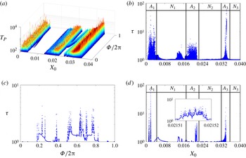
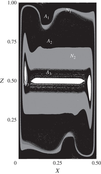
particles. Figure 5 shows the distribution of
 ${\it\tau}=T_{P}/T_{SL}$
as a function of
 ${\it\Phi}$
and
 $X_{0}$
. Three seemingly fractal distributions of
 ${\it\tau}$
are found in the regions referred to as
 $A_{i},\ i=1,2,3$
. They indicate the presence of chaotic scattering regions explored, be it transiently or not, by the tracers. Here
 $A_{1}$
corresponds to a region including the proximity of the walls. Here
 $A_{2}$
and
 $A_{3}$
correspond to the proximity of former homoclinic and heteroclinic loops
 ${\it\Gamma}_{1,j}$
and
 ${\it\Gamma}_{2,j}$
,
 $j=1,2$
. The regions
 $A_{i}$
are delimited by intermediate regions with a smooth dependence on
 ${\it\Phi}$
and smooth variations of
 ${\it\tau}$
. Such regions are referred to as
 $N_{i},\ i=1,2,3$
in figures 5 and 6. The central zone around the centre of the cavity is not treated here because of the huge return times associated with nearly vanishing velocities.
Trajectories inside the
 $A_{i}$
areas (in black) associated with singularities in figure 5. Here
 $N_{i}$
corresponds to the trajectories inside the non-hyperbolic areas (in grey). Here
 $i=1,2,3$
and
 $\mathit{Ra}=1.625\times 10^{8}$
.

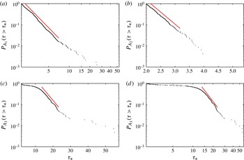
Figure 7 shows the cumulative probability distributions
 $P({\it\tau}>{\it\tau}_{\ast })$
for the normalised return time
 ${\it\tau}$
to be larger than a given value
 ${\it\tau}_{\ast }$
. Only events for which
 ${\it\tau}>2$
are taken into account. Two possible asymptotic scalings can be expected for
 $P({\it\tau}>{\it\tau}_{\ast })$
. An exponential decay of the form
 $P({\it\tau}>{\it\tau}_{\ast })\simeq \text{e}^{-{\it\alpha}{\it\tau}_{\ast }}$
would indicate hyperbolic scattering, while an algebraic decay of the form
 $P({\it\tau}>{\it\tau}_{\ast })\simeq {\it\tau}_{\ast }^{-{\it\lambda}}$
would indicate non-hyperbolic scattering (Ott & Tél Reference Ott and Tél1993). This distinction is crucial for a description of the long-time properties of the mixing process. In addition, it allows us to establish a classification of the different dynamics occurring in different spatial zones of the flow.
Cumulative probabilities
 $P({\it\tau}>{\it\tau}_{\ast })$
where
 ${\it\tau}=T_{P}/T_{SL}$
(see the text) for different regions
 $A_{1}$
,
 $A_{2}$
,
 $A_{3}$
and
 $\mathit{Ra}=1.625\times 10^{8}$
: (a)
 $A_{1}$
, algebraic fit with exponent
 ${\it\lambda}=3.3$
; (b)
 $A_{2}$
, exponential fit with
 ${\it\alpha}=1.15$
; (c)
 $A_{3}$
, exponential fit with
 ${\it\alpha}=0.10$
; (d) same as (c) in log–log plot, showing a better algebraic fit with
 ${\it\lambda}=4.11$
. The corresponding areas are shown in figure 5(b) and their representation in the physical space in figure 6.

In the region
 $A_{1}$
,
 $P({\it\tau}_{\ast })$
scales algebraically, see figure 7(a). This strongly suggests that the particles departing from
 $A_{1}$
are advected through an area where all invariant sets possess non-hyperbolic properties. The probability distribution in region
 $A_{2}$
almost perfectly fits an exponential decay (figure 7
b). Therefore, we can expect the dynamics to be hyperbolic. Finally,
 $P({\it\tau}_{\ast })$
in region
 $A_{3}$
shows a mixed exponential/algebraic scaling (figure 7
d). Since the algebraic fit is valid over a wider range of values of
 ${\it\tau}_{\ast }$
than the exponential one (see figure 7
c), it suggests that
 $A_{3}$
is dominated by non-hyperbolic dynamics for larger times but still displays signs of near-hyperbolic dynamics on shorter timescales, at least for the observation times considered here. As we shall see next, hyperbolic properties of
 $A_{2}$
and
 $A_{3}$
are related to the breakdown of the homoclinic and heteroclinic loops
 ${\it\Gamma}_{i,j}$
in the unsteady regime, whereas non-hyperbolic properties are associated with the survival of KAM tori and to a lesser degree with the no-slip condition at the walls. The next section is devoted to an explanation of all of these statistical properties from a deterministic point of view.
4. Properties of invariant sets
4.1. Definition of the stroboscopic section
 ${\it\Pi}$

Taking advantage of the time-periodicity of the flow field, the dynamics of the tracers can be studied using a stroboscopic map
 ${\rm\pi}$
transporting the position of any tracer in
 $\mathscr{D}$
onto its position one period
 $T_{0}$
later. In this representation, (3.1) is reduced to an autonomous two-dimensional map
 ${\rm\pi}:\mathscr{D}\rightarrow \mathscr{D}$
such that
 ${\rm\pi}(\boldsymbol{X}_{0})={\it\phi}^{T_{0}}(\boldsymbol{X}_{0})$
,
 ${\it\phi}^{T_{0}}$
being the propagator over one period
 $T_{0}$
. We define the stroboscopic section of a given trajectory passing through
 $\boldsymbol{X}_{0}$
as
 ${\it\Pi}=\{{\rm\pi}^{n}(\boldsymbol{X}_{0})\}_{n\in \mathbb{Z}}$
. Note that since the flow is incompressible, the continuous-time flow
 ${\it\phi}^{t}$
is area-preserving, hence the initial phase
 ${\it\Phi}$
of the velocity field can be chosen arbitrarily in
 $[0,2{\rm\pi}[$
to define
 ${\it\Pi}$
. Furthermore, the harmonic forcing is not external but intrinsic to the flow since it is determined by the Hopf bifurcation occurring at
 $\mathit{Ra}=\mathit{Ra}_{c}$
.
4.2. Numerical tools in the stroboscopic section
An orbit crossing the stroboscopic section
 $n$
times before returning to its original position defines
 $n$
periodic points of period
 $n$
in
 ${\it\Pi}$
. The numerical identification of such periodic points is based on two numerical algorithms: a standard Newton–Raphson algorithm, and an alternative algorithm described in the appendix A. The convergence criterion for both algorithms is
 $\Vert {\rm\pi}^{n}(\boldsymbol{X})-\boldsymbol{X}\Vert _{\infty }<10^{-10}$
. A Jacobian matrix is evaluated at order one by releasing two extra tracers in the neighbourhood of the reference periodic point and monitoring the separation versus time. Depending on the imaginary part of the spectrum of this matrix, we can distinguish whether the periodic point is a centre or a saddle. Therefore, eigenvalues are not expected to be accurate at all. However, it is expected that the nature of the identified periodic point (saddle or centre) will still be reflected in the imaginary part of the eigenvalues. Once an unstable periodic point is identified, a disk of radius
 $10^{-7}$
seeded with 100 tracers distributed on 10 concentric circles is placed around this point. Tracers are then tracked in
 ${\it\Pi}$
in backward and forward time in order to highlight the stable and unstable manifolds of each hyperbolic point.
4.3. Destabilisation of homoclinic and heteroclinic connections
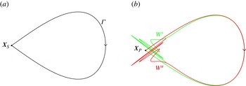
As long as the Lagrangian system is autonomous, the stable (
 $W^{s}$
) and unstable (
 $W^{u}$
) manifolds of a homoclinic saddle point
 $\boldsymbol{X}_{S}$
coincide and form a homoclinic loop
 ${\it\Gamma}$
. When subject to harmonic forcing, the saddle point becomes a periodic orbit, i.e. a periodic point
 $\boldsymbol{X}_{P}$
in
 ${\it\Pi}$
whose manifolds
 $W^{u}(\boldsymbol{X}_{P})$
and
 $W^{s}(\boldsymbol{X}_{P})$
no longer coincide. However, if they cross transversally at least once in
 ${\it\Pi}$
it is known that they cross an infinite countable number of times (Poincaré Reference Poincaré1892; Guckenheimer & Holmes Reference Guckenheimer and Holmes1983; Wiggins Reference Wiggins1988). This gives rise to a so-called homoclinic tangle consisting of an infinity of lobes of equal area. The conservation of the areas is a direct consequence of the Hamiltonian structure of (3.2) and implies a complex foliation of the lobes. Periodic points are dense in the chaotic region and the dynamics restrained to this area displays hyperbolic mixing properties. The transport from lobe to lobe is responsible for the mixing properties in the vicinity of the original homoclinic loop
 ${\it\Gamma}$
(Ottino Reference Ottino1990; Rom-Kedar et al.
Reference Rom-Kedar, Leonard and Wiggins1990). This is illustrated in figure 8 where the manifolds are depicted over an observation time long enough to display a few transversal crossings. The same scenario is valid for the destabilisation of heteroclinic orbits.
(a) Sketch of a homoclinic connection
 ${\it\Gamma}$
from a fixed point
 $\boldsymbol{X}_{S}\ ({\it\varepsilon}=0)$
. (b) Transversal intersections of the stable (
 $W^{s}$
) and unstable (
 $W^{u}$
) manifolds of the associated periodic point
 $\boldsymbol{X}_{P}$
lead to a homoclinic tangle (
 ${\it\varepsilon}>0$
).

Melnikov functions are a convenient tool to predict whether the stable and unstable manifolds of a periodic point cross each other or not (Melnikov Reference Melnikov1963). Such a function is proportional to the signed
 $O({\it\varepsilon})$
distance between the stable and unstable manifolds of the hyperbolic point:
 $$\begin{eqnarray}M(t_{0})=\int _{-\infty }^{\infty }\det [\boldsymbol{U}_{0}(\boldsymbol{X}_{0}(t)),\boldsymbol{U}_{P}(\boldsymbol{X}_{0}(t),t+t_{0})]\,\text{d}t,\end{eqnarray}$$
where
 $\boldsymbol{U}_{0}$
corresponds to the (unstable) steady velocity field evaluated along the homoclinic loop
 ${\it\Gamma}$
,
 $\boldsymbol{X}_{0}(t)$
corresponds to a trajectory along
 ${\it\Gamma}$
parametrised by time
 $t$
, and
 $\boldsymbol{U}_{P}$
is the finite-amplitude perturbation from
 $\boldsymbol{U}_{0}$
. If
 $M(t_{0})$
vanishes for some isolated values of
 $t_{0}$
, the stable and unstable manifolds intersect transversally and a homoclinic tangle exists in the vicinity of
 ${\it\Gamma}$
. The mass transport from lobe to lobe associated with the homoclinic tangle produces Lagrangian mixing. The integral of the unsigned Melnikov function provides a first order approximation of the area covered by the lobes (Rom-Kedar et al.
Reference Rom-Kedar, Leonard and Wiggins1990; Hackborn, Ulucakli & Yuster Reference Hackborn, Ulucakli and Yuster1997).
The Melnikov function in (4.1) can be redefined as function of the phase variable
 ${\it\Phi}=2{\rm\pi}t_{0}/T_{0}\in [\!0,2{\rm\pi}\ $M$
with
 $\mathit{Ra}$
, we furthermore consider the normalisation of the Melnikov function given by
 $$\begin{eqnarray}{\it\Lambda}_{i,j}({\it\Phi})=\frac{M_{i,j}({\it\Phi})}{\displaystyle \int _{0}^{2{\rm\pi}}|M_{i,j}({\it\Phi})|\,\text{d}{\it\Phi}},\end{eqnarray}$$
where the subscripts
 $i$
and
 $j$
refer to the index of the homoclinic or heteroclinic loop as defined in § 3.2. The Melnikov functions are computed numerically by direct evaluation of the integral along
 ${\it\Gamma}$
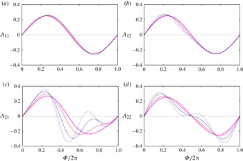
in (4.1). Figure 9 shows the normalised Melnikov functions for the homoclinic loops
 ${\it\Gamma}_{1,1}$
and
 ${\it\Gamma}_{2,2}$
and the heteroclinic connections
 ${\it\Gamma}_{1,2}$
and
 ${\it\Gamma}_{2,1}$
, each of them computed for four values of
 $\mathit{Ra}>\mathit{Ra}_{c}$
. In all cases
 ${\it\Lambda}({\it\Phi})$
vanishes at least twice, indicating transversal intersections of the manifolds, and hence the existence of chaotic tangles via the break-up of the connections.
Normalised Melnikov functions
 ${\it\Lambda}_{i,j}$
associated with saddle points of the unstable steady state for
 $\mathit{Ra}=1.587\times 10^{8}$
(—),
 $\mathit{Ra}=1.590\times 10^{8}$
(
 $-$
 $-$
),
 $\mathit{Ra}=1.600\times 10^{8}$
(
 $-\cdot$
) and
 $\mathit{Ra}=1.625\times 10^{8}$
(
 $\cdot$
). The presence of isolated zeros shows the existence of homoclinic/heteroclinic tangles.

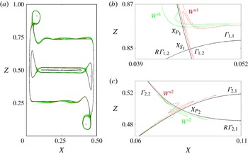
Both unstable periodic points
 $\boldsymbol{X}_{P_{1}}$
and
 $\boldsymbol{X}_{P_{2}}$
, associated with
 $\boldsymbol{X}_{S_{1}}$
and
 $\boldsymbol{X}_{S_{2}}$
respectively, give rise to the tangles shown in figure 10 for the case
 $\mathit{Ra}=1.587\times 10^{8}$
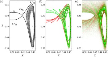
. It is noteworthy from figure 10 that for
 $\mathit{Ra}$
closest to
 $\mathit{Ra}_{c}$
, the distance
 $|\boldsymbol{X}_{P_{i}}-\boldsymbol{X}_{S_{i}}|$
is larger for
 $i=1$
than for
 $i=2$
. This is due to the intensity of the oscillations of
 $\boldsymbol{U}_{\boldsymbol{P}}$
being much larger near
 $\boldsymbol{X}_{S_{1}}$
than near
 $\boldsymbol{X}_{S_{2}}$
, as is already clear from figure 3. Note the similarities between figure 10(b,c) and the sketch in figure 8(b). All destabilised homoclinic/heteroclinic connections identified in figure 5 induce fluid mixing, at least in a finite-size neighbourhood. Tracers seeded in the close vicinity of such hyperbolic points appear to spread over an area comparable to that of the lobes, so that mixing is only partial for
 $\mathit{Ra}=1.587\times 10^{8}$
(figure 10
a). This is typical of the existence of transport barriers in an
 $O({\it\varepsilon})$
vicinity of the homoclinic tangle, as investigated in the following subsections. The case of higher
 $\mathit{Ra}$
(when
 ${\it\varepsilon}$
is no longer small) will be treated in the last section of the paper.
(a) Spreading of particles initially placed close to the hyperbolic fixed points
 $X_{P_{1}}$
and
 $X_{P_{2}}$
. Circles, fixed points associated with the unstable steady state at
 $\mathit{Ra}=1.587\times 10^{8}$
; solid lines, homoclinic and heteroclinic orbits; black dots (red online), forward time integration; grey dots (green online), backward time integration. Both disks are composed of
 $10^{4}$
particles and are integrated over 50 periods in
 ${\it\Pi}$
following the procedure described in § 4.2. (b,c) Enlarged views of the crossing manifolds originating from
 $X_{P_{1}}$
(b) and
 $X_{P_{2}}$
(c) on shorter integration times. Note that
 $X_{P_{2}}$
and
 $X_{S_{2}}$
are nearly indistinguishable.

4.4. Periodic points in the stroboscopic section
Because of incompressibility, periodic points in
 ${\it\Pi}$
can only be saddles or centres, while sinks are precluded. Because mixing is related to stretching by the velocity field, local mixing can only occur in the immediate vicinity of hyperbolic saddle points in
 ${\it\Pi}$
, which in continuous time correspond to either saddle points or unstable periodic orbits (UPOs), but not around centres. As seen in the previous subsection, the periodic points corresponding to saddle points of the base flow all induce mixing in the unsteady regime. In fact, all hyperbolic points identified in
 ${\it\Pi}$
have the property to mix fluid over some (a priori unknown) finite-size area. Within the mixing zone corresponding to one given periodic point
 $\boldsymbol{X}_{P}$
, a dense aperiodic trajectory linking any two points should exist, as a consequence of the chaotic nature of mixing. Hence, any point within that zone should be arbitrarily close to both
 $W^{s}(\boldsymbol{X}_{P})$
and
 $W^{u}(\boldsymbol{X}_{P})$
. In other words the mixing area associated with a given periodic point
 $\boldsymbol{X}_{P}$
in
 ${\it\Pi}$
coincides with the closure of its stable and unstable manifolds, themselves being interpreted as the skeleton of the hyperbolic mixing zone. This point of view is prominent in the study by Feudel et al. (Reference Feudel, Witt, Gellert, Kurths, Gregobi and Sanjuán2005) who suggest that the total area occupied by mixing in the system corresponds to the closure of a bundle of manifolds.
Here we wish to determine numerically the mixing zone associated with each periodic point that can be identified in
 ${\it\Pi}$
, by tracing out its stable and unstable manifolds and measuring the area covered by their intertwining. This task is ambitious since (i) there are infinitely many periodic points of arbitrary high period and (ii) the infinitely convoluted geometry of these manifolds requires in practice a coarse-graining procedure. Moreover, each mixing zone contains new periodic points whose manifolds cover the same area as the periodic point originally considered to define the mixing zone. Hence redundancies are expected in practice. The benefit of this approach is an accurate a priori prediction of the various mixing zones of the flow from a deterministic point of view, rather than from the statistical a posteriori analysis of § 3. In addition, as we shall see, in practice a finite number of periodic points is enough to obtain a quantitatively satisfying coverage of all mixing zones, and hence to determine to which degree mixing in the cavity can be considered as complete or incomplete. It is moreover expected that the chaotic area increases with
 $\mathit{Ra}$
and we suggest in what follows a method to quantify it.
The method relies on the computation of spreading maps associated with every individual periodic point in
 ${\it\Pi}$
. We first begin by extracting numerically as many periodic points as possible using the method explained in § 4.2. We introduce the disk
 $\mathscr{B}_{i}$
of radius
 $d$
centred on a periodic point
 $P_{i}$
of period
 $T_{i}$
. A finite number of tracers (
 $\mathscr{B}_{i}^{\prime }$
) is chosen in
 $\mathscr{B}_{i}$
as in § 4.2. The partial spreading map associated with
 $P_{i}$
is defined as
 $$\begin{eqnarray}S_{i}=\mathop{\bigcup }\limits_{|q|\leqslant Q}{\rm\pi}^{qT_{i}}(\mathscr{B}_{i}^{\prime }).\end{eqnarray}$$
We later define the total spreading map as the union of all partial spreading maps for a given value of
 $\mathit{Ra}$
:
 $$\begin{eqnarray}{\it\Sigma}_{n}=\mathop{\bigcup }\limits_{P_{i}\in \mathscr{R}_{n}}S_{i},\end{eqnarray}$$
where
 $\mathscr{R}_{n}$
is the set of all identified periodic points whose period is less than
 $nT_{0}$
. In the present investigation, we used
 $d=10^{-7}$
,
 $Q=50$
and
 $n=40$
, as a compromise between accuracy and computational effort (see § 5).
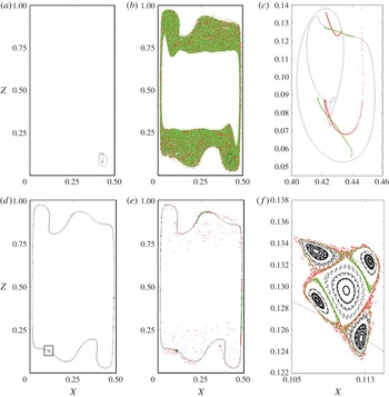
Two examples of partial spreading maps for
 $\mathit{Ra}=1.625\times 10^{8}$
. (a,d) UPOs (lines) and associated periodic points (open dots) in
 ${\it\Pi}$
. (b,e) partial spreading map for the periodic points in
 ${\it\Pi}$
. (c,f) zoom on the manifolds of the periodic points. Forward iterations shown in black (red online), backward in grey (green online). (a–d) tangle associated with a periodic point with period
 $T=2T_{0}$
. (d–f) non-mixing island associated with resonant streamline of period
 $T=6T_{0}$
. ( f) is a close-up of the rectangle in (a).

Two examples of partial spreading maps are shown in figure 11. The corresponding UPO (a,d), the associated partial spreading map (b,e) and a zoom on its stable/unstable manifolds (c,f) are successively displayed.
-
(a) The first UPO (first row) has period
$2T_{0}$
and is associated with two periodic points of period two. The UPO is entirely located in one of the two detached corners. Even if it occupies a small fraction of the cavity (figure 11
a), the mixing induced by the periodic point is considered as efficient since it covers a comparatively large area that coincides with
$A_{2}$
(figure 11
b). It is clear from figure 11(c) that the stable and unstable manifolds of these points cross transversally and that the scenario of § 4.3 is reproduced even in the absence of homoclinic loop. -
(b) The second UPO shown in figure 11(d) (solid line) has period
$6T_{0}$
and is associated with six periodic points in
${\it\Pi}$
. As can be seen from figure 11(e), the mixing induced by this UPO is highly inefficient even though the diameter of the UPO is comparable to the cavity size. A zoom on the topological structure around two of these periodic points is shown in figure 11( f). The vicinity of the orbit exhibits heteroclinic connections between four periodic points and the appearance of several heteroclinic tangles. However, the structure defined by the periodic points composing the heteroclinic tangles does not spread particles efficiently.


Those two examples demonstrate that the diameter of a given UPO and its mixing properties are not necessarily correlated.
4.5. Resonant streamlines
In order to highlight the dynamics inside the structure displayed in figure 11( f), we have added lines of particles inside each region lying between the saddle points represented, and propagated these new tracers in
 ${\it\Pi}$
over a time of
 $50T_{0}$
. This computation shows that if a particle starts inside the structure, it cannot escape from it. Most of those particles trace out ellipses in
 ${\it\Pi}$
. Equivalently the continuous-time dynamics is quasiperiodic and the associated trajectories form toroidal surfaces in a space–time representation. These tori are precisely the KAM tori resulting from the non-integrability of the Hamiltonian system (3.1). These structures are not associated with an unstable manifold and, hence, are not repelling. Tracers in a neighbourhood of KAM tori are known to ‘stick’, which results in increased residence times. As a consequence of this stickiness effect, they are commonly interpreted as the origin for non-hyperbolicity in the statistics of return times. The KAM tori define strict material barriers in
 ${\it\Pi}$
(Ottino Reference Ottino1990), forbidding transport from one mixing zone to another one.
In the steady regime any streamline, parametrised by its closure time
 $T_{SL}$
, acts as a barrier to transport. As the flow becomes oscillatory, the periodic dynamics of tracers becomes in principle quasiperiodic with two periods, one close to
 $T_{SL}$
and the second being
 $T_{0}$
. The KAM theorem (see e.g. Guckenheimer & Holmes Reference Guckenheimer and Holmes1983) ensures that for
 $0<{\it\varepsilon}\ll 1$
a measurable set of toroidal trajectories are preserved, allowing for the presence of non-mixing islands. The condition for toroidal trajectories, i.e. material barriers to persist is that the ratio
 ${\it\delta}=T_{SL}/T_{0}$
be sufficiently far from any rational number
 $p/q$
(with
 $p$
and
 $q$
not too large in practice when dealing with computer arithmetics). This predictive argument associates transport barriers in the unsteady regime with certain streamlines of the steady base flow that are more robust to unsteady forcing than others. Streamlines for which
 ${\it\delta}$
is close to a rational number
 $p/q$
can lock on a periodic motion with
 $T_{SL}=pT_{0}/q$
. Such resonant streamlines undergo a saddle–node bifurcation giving rise to the alternation between saddles (hyperbolic orbits) and centres (elliptic orbits) illustrated in figure 11( f). Manifolds originating from the saddle points form homoclinic and heteroclinic tangles enclosing the elliptic points and are responsible for the emergence of a stochastic layer in which mixing occurs locally. Similarly, other resonances can occur inside each region surrounded by a heteroclinic tangle, resulting in a complex tapestry of barriers and stochastic layers. The width of these stochastic layers is usually smaller with increasing values of
 $q$
but grows with
 ${\it\varepsilon}$
. Several neighbouring layers predicted by this arithmetic criterion can hence overlap as
 ${\it\varepsilon}$
increases, hence producing a wider mixing zone in which diffusive motion of the tracers is possible (Cencini, Cecconi & Vulpiani Reference Cencini, Cecconi and Vulpiani2010; Mitchell & Grigoriev Reference Mitchell and Grigoriev2012).
Resonant streamlines, via the formation of heteroclinic tangles, are naturally associated with periodic points in
 ${\it\Pi}$
, be they hyperbolic or elliptic. Hyperbolic and elliptic points appear together via saddle–node bifurcations and hence come in pairs. Conversely, once a periodic point is identified in
 ${\it\Pi}$
, it is not trivial to distinguish whether it is originally associated with the resonance of a given streamline or with one of the tangles predicted by Melnikov analysis. The KAM theorem suggests that non-resonant tori should be present in the vicinity of most elliptic periodic points, implying non-mixing islands (Wiggins & Ottino Reference Wiggins and Ottino2004) and thus non-hyperbolic statistics. The question remains however non-trivial in the case of hyperbolic points. The distinction is further complicated by the fact that periodic points can undergo bifurcations as
 ${\it\varepsilon}$
is increased. The simplest approach to this question is to check, orbit by orbit, whether the resonance criterion
 $$\begin{eqnarray}T_{SL}=pT_{0}/q\end{eqnarray}$$
is verified or not. Considering again the segment
 ${\bf\chi}$
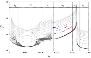
defined in § 3.2, we plot in figure 12 the period of all periodic orbits crossing
 ${\bf\chi}$
versus the crossing coordinate
 $X_{0}$
, together with the return times
 $T_{SL}$
associated with the steady base flow. Saddle points are shown as points, elliptic points as open circles. The periodic points whose period falls close to integer multiples of
 $T_{SL}(X_{0})$
should correspond to the thickest resonant tori with
 $q=1$
. The value of
 $\mathit{Ra}=1.625\times 10^{8}$
is chosen for comparison with the statistical analysis of § 3.3.
Plot of the period of all periodic orbits crossing
 ${\bf\chi}$
versus the crossing coordinate
 $X_{0}$
, together with the return times
 $T_{SL}$
associated with the steady base flow. Solid lines:
 $T_{SL}$
as a function of
 $X_{0}$
with integer multiples
 $n\times T_{SL}$
for
 $\mathit{Ra}=1.625\times 10^{8}$
. Black dots (red online): UPOs crossing the segment
 ${\bf\chi}=\{X\in [0,0.05],Z={\textstyle \frac{1}{2}}\}$
. Circles (blue online): elliptic periodic orbits. Grey dots: distribution of return times
 $T_{P}({\it\Phi},X_{0})$
(from figure 5
b). Here
 $A_{i}$
and
 $N_{i}$
,
 $i=1,2,3$
correspond to the areas defined in figure 6.

The distribution of the periods is of course limited by the number of UPOs found. However even with 168 orbits this distribution reveals interesting features. A vast majority of the periodic orbits, both hyperbolic and elliptic, whose period is commensurate with
 $T_{SL}$
in figure 12, correspond to values of
 ${\it\delta}=T_{SL}/T_{0}=1$
to 5 and belong to the region denoted
 $N_{2}$
in § 3.3. Other elliptic points were also identified in the region
 $N_{1}$
, as well as in the region
 $A_{3}$
with
 ${\it\delta}=1$
and in
 $N_{3}$
with
 ${\it\delta}=2$
and 5. Neither hyperbolic orbits nor elliptic orbits have been detected in
 $A_{1}$
and
 $A_{2}$
using this criterion. Note that this approach is necessarily partial since it requires the periodic orbits to cross the segment
 ${\bf\chi}$
, while the choice of
 ${\bf\chi}$
is convenient but still arbitrary.
A direct interpretation of figure 12 in connection with the statistics of § 3.3 is now possible. The presence of elliptic orbits satisfying the criterion (4.5) implies the proximity of non-resonant orbits (KAM tori or non-mixing islands). By default, periodic orbits which according to (4.5) do not come from resonances, are most likely embedded in the tangles associated with the destabilisation of homo/heteroclinic loops as in § 4.3. Consequently the region
 $N_{2}$
is expected to be populated by many non-hyperbolic objects such as the non-mixing islands of figure 11( f). Here
 $N_{1}$
and
 $N_{3}$
contain a small but non-zero number of such elliptic orbits and, hence, should contain a few non-mixing islands too. Here
 $A_{3}$
contains very few low-period elliptic orbits, which explains that its non-hyperbolic statistical properties emerge for large times. Here
 $A_{2}$
does not show any such resonance, which by default is consistent so far with its hyperbolic nature. In addition, the only periodic points identified in
 $A_{2}$
are hyperbolic and occur close to the fractal distribution of the return times
 $T_{P}$
, which is consistent with the picture of a homo/heteroclinic tangle of figure 8. Yet it is fair to recall that the statistics in question are also dependent on the choice of the segment
 ${\bf\chi}$
, so that non-hyperbolicity is not strictly ruled out provided a few non-mixing regions exist that do not cut
 ${\bf\chi}$
. This case will be examined in further detail in § 5 using spreading maps. The case of
 $A_{1}$
, which does not feature resonances according to figure 12 but still shows clear non-hyperbolic statistics, seems contradictory. This case is however peculiar since this region also includes the streamlines closest to the walls. Because of the no-slip condition, the velocity
 $\boldsymbol{U}$
vanishes at the wall, and hence the period
 $T_{SL}$
diverges too, making resonances impossible. Here
 $A_{1}$
is thus expected without any preliminary analysis to display strongly non-hyperbolic statistics since the wall itself, as well as all neighbouring streamlines, can be interpreted as a non-resonant KAM torus.
We pay particular attention to some of the periodic points represented in figure 12 both as centres and saddles, mainly distributed in the region
 $N_{2}$
. We cannot certify the stability of those periodic points through the finite-difference computation of § 4.2. Because of the fractal configuration of the KAM tori alternating with mixing areas, the perturbed trajectories used for the linearisation can very well be located outside the zone under investigation. They can land on another KAM torus (the point is identified as a centre) or in a locally mixing area (it is detected as a saddle). This ambiguous property is not a numerical artefact but reflects the multiscale structure of
 ${\it\Pi}$
. Note that this is in any case a minor issue since these points never contribute significantly to the spreading of the tracers.
The fine-scale coexistence of hyperbolic and non-hyperbolic regions is finally illustrated for
 $\mathit{Ra}=1.625\times 10^{8}$
around the vortex in the middle-right of the cavity, i.e. around
 $X=Z\approx 0.45$
, see figure 13. This area involves mainly the regions
 $A_{3}$
and
 $N_{3}$
as well as the homoclinic loop
 $R{\it\Gamma}_{2,2}$
. Figure 13(a) shows all periodic orbits identified in the continuous-time representation, along with the homo/heteroclinic loops. Figure 13(b,c) show the spreading maps associated with all those orbits for a short and a long observation time, respectively. Note that the heteroclinic loop
 ${\it\Gamma}_{2,1}$
acts as a barrier isolating the central region of the cavity from the rest of the flow. It is visually clear from figure 13 that the complete or incomplete character of the mixing, as well as the associated statistics, result from a compromise between the hyperbolic tangle predicted by the Melnikov function
 ${\it\Lambda}_{2,2}$
and the many KAM tori (barriers) remaining in the flow for this value of
 $\mathit{Ra}$
.
(a) Periodic orbits (grey lines) and corresponding periodic points in
 ${\it\Pi}$
(circles) identified numerically in the vicinity of
 $R{\it\Gamma}_{2,2}$
for
 $\mathit{Ra}=1.625\times 10^{8}$
. Black lines:
 ${\it\Gamma}_{21}$
,
 $R{\it\Gamma}_{2,2}$
and
 $R{\it\Gamma}_{2,1}$
. (b) Stable (grey, green online) and unstable (black, red online) manifolds of these periodic points. The main homoclinic tangle originates from
 $X_{P_{2}}$
and surrounds non-mixing islands and stochastic layers formed by resonant streamlines. (c) Same as (b) with partial spreading maps superimposed. Stochastic layers overlap leading to a complex mixing zone.

5. Mixing versus
$\mathit{Ra}$

The total spreading maps defined in § 4.4 offer a more global vision of the regions affected or not by mixing for a given value of
 $\mathit{Ra}$
. Figure 14 displays for several values of
 $\mathit{Ra}$
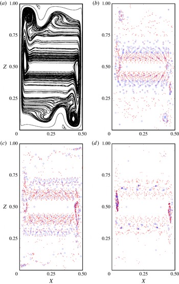
the hyperbolic periodic points used for the computation of the manifolds. The spreading maps
 ${\it\Sigma}_{n}$
are computed in practice by paving the domain with square cells of area
 ${\rm\Delta}X^{2}$
, and counting the number of tracers that have passed through each cell over a given time horizon
 $T_{obs}=QT_{0}$
, with
 $Q=50$
. The resulting maps are shown in figure 15 for increasing values of
 $\mathit{Ra}$
. Cells occupied by at least one or more tracers are represented in black, while cells that have remained empty over the time interval
 $[0:T_{obs}]$
are left blank. The black cells are by construction connected to the hyperbolic periodic points of figure 14 by their stable/unstable manifolds, which as seen in the previous section are parts of chaotic tangles. Black cells thus define the mixing regions within the coarse-graining approximation.
(a) UPOs identified for
 $\mathit{Ra}=1.6\times 10^{8}$
. (b), (c) and (d) Associated periodic points represented with filled circles (saddle points, red online) or open circles (elliptic points, blue online) for (b)
 $\mathit{Ra}=1.6\times 10^{8}$
, (c)
 $\mathit{Ra}=1.625\times 10^{8}$
and (d)
 $\mathit{Ra}=2.05\times 10^{8}$
.

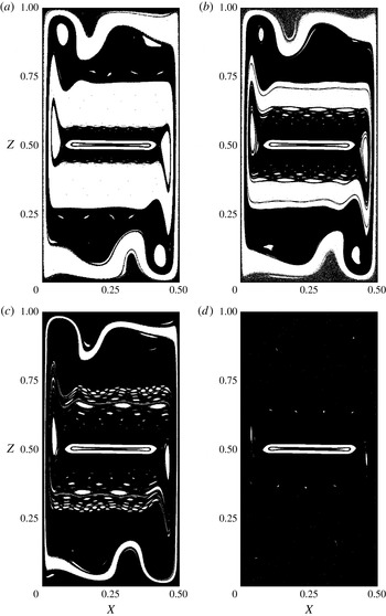
Total spreading maps
 ${\it\Sigma}_{n=40}$
for (a)
 $\mathit{Ra}=1.59\times 10^{8}$
, (b)
 $\mathit{Ra}=1.6\times 10^{8}$
, (c)
 $\mathit{Ra}=1.625\times 10^{8}$
and (d)
 $\mathit{Ra}=2.05\times 10^{8}$
.

The lowest values of
 $\mathit{Ra}$
displayed in figure 15(a–c) feature white stripes whose width and number diminish with increasing
 $\mathit{Ra}$
. The dynamics of the tracers inside those regions is strictly quasiperiodic and these zones are interpreted as non-mixing. These regions are isolated from the other mixing regions (represented in black) by clear material barriers. White holes embedded in a black chaotic sea are the signature of non-mixing islands such as in figure 11( f). They can be isolated or form chains of non-mixing islands exhibiting an alternation of hyperbolic points and centres typical of KAM resonances and already visible in figure 14. A robust white zone remains for all values of
 $\mathit{Ra}$
in the central zone of the cavity. As mentioned previously, the velocity magnitude is slow because of the antisymmetry of the velocity field. Mixing, if it occurs, is extremely slow and is not observed in finite-time computations. It is therefore interpreted in the reminder of the paper as a robust non-mixing zone. The case of
 $\mathit{Ra}=1.625\times 10^{8}$
discussed in § 4.5 is shown in figure 15(c). As predicted from the distribution of elliptic points in figure 12, the region previously denoted
 $N_{2}$
contains a multiscale tapestry of non-mixing islands that is associated with strongly non-hyperbolic dynamics, in other words it can be qualified as a very ‘sticky’ region. The region
 $A_{2}$
was suggested, from the scattering statistics of § 3 based on the test section
 ${\bf\chi}$
, to be a hyperbolic region. In the previous Subsection a note of caution was addressed, linked to the possible existence of KAM tori that would not cross
 ${\bf\chi}$
and hence heavily alter the statistics. Figure 15(c) reveals a small number of isolated white holes in
 $A_{2}$
, yet no clear white regions inside the vortex corresponding to the homoclinic loop
 ${\it\Gamma}_{1,1}$
: at least within an accuracy
 $O({\rm\Delta}X)$
. This justifies why the homoclinic tangle associated with
 ${\it\Gamma}_{1,1}$
, where the forcing by
 $\boldsymbol{U}_{\boldsymbol{P}}$
has strongest amplitude, appeared as hyperbolically mixing. This contrasts with the other homoclinic tangle associated with
 ${\it\Gamma}_{2,2}$
and displayed in figure 13, which for the same value of
 $\mathit{Ra}$
features many non-mixing islands and thus strong non-hyperbolic statistics. The relatively small white holes identified near the border between regions
 $A_{2}$
and
 $N_{1}$
are expected to destroy the hyperbolic nature of
 $A_{2}$
by inducing over longer observation times an algebraic rather than exponential decay of the return-time statistics. This remains however to be confirmed using much longer simulations. For lower values of
 $\mathit{Ra}$
, that same region
 $A_{2}$
displays a few white holes, i.e. the presence of KAM tori, within the corner vortex inside
 ${\it\Gamma}_{1,1}$
, in a way similar to figure 13. For the largest value
 $\mathit{Ra}=2.05\times 10^{8}$
, within the observation times considered here, almost all barriers have disappeared except in the centre of the cavity. Increasing
 $\mathit{Ra}$
mainly increases the forcing amplitude, while the forcing frequency remains constant at leading order. The increasing amplitude reduces stickiness effects associated with KAM tori because more and more of these tori resonate. In theory the last surviving KAM torus should correspond to the most irrational value of
 ${\it\delta}$
(in terms of its approximation by rational fractions). This prediction however does not take into account the steady ‘streamline’ (defined as such since associated with the integrability condition
 ${\it\Psi}=\text{const}.$
), i.e. the walls, which will remain non-hyperbolic for all values of
 $\mathit{Ra}$
even far beyond the periodic regime.
Total spreading maps can be used to provide a quantitative estimation of how complete mixing is for a given value of
 $\mathit{Ra}$
. The area covered by the bundle of manifolds originating from all UPOs of period less than
 $nT_{0}$
, is computed by monitoring the fraction of cells of area
 ${\rm\Delta}X^{2}$
visited by at least one particle over the observation time
 $T_{obs}=QT_{0}$
. The cell size
 ${\rm\Delta}X$
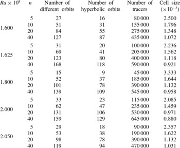
is chosen such that the number of cells equals the number of released tracers times the number of passages in
 ${\it\Pi}$
. If spreading were homogeneous, each box would be filled. The box resolution is therefore a function of
 $n$
, the longest period among all of the UPOs considered here. In this coarse-grained approach, the number of cells filled at least with one tracer is
 $B\leqslant 1/(2{\rm\Delta}X^{2})$
as in Stremler (Reference Stremler2008) and Chabreyrie et al. (Reference Chabreyrie, Chandre, Singh and Aubry2011). The total fraction
 $C$
of chaos is defined as the area covered by the
 $B$
cells normalised by the surface of the cavity:
 $C=2B{\rm\Delta}X^{2}$
. If
 $C$
reaches unity, we expect that most KAM tori have become resonant, or have overlapped. This extreme case corresponds to complete mixing.
A note of caution about the use of time-discretised numerical simulations is welcome at that stage. Because the mixing regions are intrinsically chaotic and, hence, display sensitivity to initial conditions, the computation of the stable or unstable manifolds is expected to show errors that increase exponentially with time, no matter the accuracy of the temporal scheme. Fortunately, the long-time influence on the global spreading maps is less dramatic, as their topology is mostly dependent on the location of the non-mixing islands. Since KAM tori are associated with strictly zero Lyapunov exponents, the accuracy of the whole protocol is only limited by the accuracy with which the tori are represented numerically, as well as by the coarse-graining parameters. In practice, time-stepping algorithms are characterised by diffusing properties (see the closure of streamlines documented in § 3.1) which defines a numerical Lyapunov exponent. That numerical exponent is usually very small in practice yet sets a limit to the duration over which tracers can be reliably tracked.
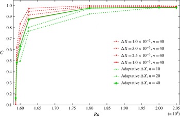
The total chaotic fraction is shown in figure 16 as a function of
 $\mathit{Ra}$
, parametrised by
 $n$
and the cell size. Varying
 $n$
allows one to distinguish the contribution to total mixing by shorter period UPOs from that by longer period ones. The general conclusion from figure 16 is that the fraction of Lagrangian chaos in the cavity smoothly increases from 0 % near
 $\mathit{Ra}_{c}$
towards almost 100 % for
 $\mathit{Ra}=2.05\times 10^{8}$
. Whereas the spreading maps depend by construction on the phase
 ${\it\Phi}$
chosen to define the stroboscopic section
 ${\it\Pi}$
, the quantity
 $C$
represents a normalised area, which because of incompressibility does not depend on
 ${\it\Phi}$
. Low-period UPOs appear to contribute most significantly to the total chaotic fraction
 $C$
, yet UPOs of larger period are also quantitatively significant. This trend progressively disappears for increasing
 $\mathit{Ra}$
. The fact that
 $C$
stays bounded strictly below 100 % is attributed to the robust non-mixing zone at the centre of the cavity, where the motion of the tracers is too slow to exhibit mixing in a finite time.
Chaotic fraction
 $C$
versus
 $\mathit{Ra}$
. Grey (green online): computations using
 $n=40$
and cell size
 ${\rm\Delta}X$
as in table 1. Black (red online): computations using fixed mesh size
 ${\rm\Delta}X$
and varying
 $n$
. The thickest line corresponds to the case with smallest
 ${\rm\Delta}X$
and largest
 $n$
.

Periodic orbits used for the computation of the chaotic fraction
 $C(\mathit{Ra})$
shown in figure 16.

The largest value of
 $\mathit{Ra}=2.05\times 10^{8}$
displayed in figure 16 has
 $C\approx 0.98$
, i.e. nearly 100 %. Figure 15(d) visually suggests that all white stripes, i.e. all barriers to transport have disappeared, which would in addition imply that one single mixing region fills the whole cavity. The quantity
 $C$
is however not a measure of the connectedness of the spreading maps, the hypothesis that mixing is complete at this value of
 $\mathit{Ra}$
thus has to be verified using an alternative diagnostic. The next section examines more closely this suggestion by focusing mainly on
 $\mathit{Ra}=2.05\times 10^{8}$
.
6. From local to global mixing
As seen in the previous section
 $C\lesssim 1$
for
 $\mathit{Ra}=2.05\times 10^{8}$
, which indicates that the flow is locally mixing almost everywhere in the cavity at the exception of the central area. This, however, does not directly imply complete mixing in the sense of a unique, connected and space-filling mixing region. Complete mixing would imply that a dense aperiodic trajectory exists in
 ${\it\Pi}$
. In other words, almost all barriers should have disappeared and it would be possible to spread tracers throughout the whole domain by releasing them at initial time from a single given location. In this section we select one such initial location and study statistically the dynamics of the tracers for varying
 $\mathit{Ra}$
, expecting an increasingly homogeneous spreading for larger values of
 $\mathit{Ra}$
. The initial location was chosen to correspond to the periodic point
 $\boldsymbol{X}_{P_{2}}$
, already formally defined in § 3 as the destabilisation of the homoclinic fixed point
 $\boldsymbol{X}_{S_{2}}$
associated with the steady base flow. Here
 $\boldsymbol{X}_{P_{2}}$
can be defined for any arbitrary phase of the velocity field and, importantly, moves weakly with
 $\mathit{Ra}$
. The choice of
 $\boldsymbol{X}_{P_{2}}$
was largely motivated by the fact that it was easy to track in
 ${\it\Pi}$
for increasing
 $\mathit{Ra}$
(whereas continuation of
 $\boldsymbol{X}_{P_{1}}$
proved more difficult). Once identified,
 $10^{3}$
tracers are placed inside the disk
 $\mathscr{B}$
around
 $\boldsymbol{X}_{P_{2}}$
according to the protocol described in § 4.2. The computation time is extended to
 $10^{4}T_{0}$
instead of
 $50T_{0}$
as considered for the spreading maps. If the barriers separating the different mixing areas (such as
 $A_{1}$
,
 $A_{2}$
and
 $A_{3}$
defined for the case
 $\mathit{Ra}=1.625\times 10^{8}$
) have all become permeable with increasing
 $\mathit{Ra}$
, the disk of particles should asymptotically spread homogeneously in
 ${\it\Pi}$
as
 $t\rightarrow \infty$
.
The notion of spreading is now considered in a statistical sense by investigating the average and variance
 ${\it\sigma}_{Z}^{2}$
of the stochastic variable
 $Z$
describing the vertical position of each individual tracer at any given time
 $t$
. Here
 ${\it\sigma}_{Z}^{2}$
admits an upper bound which corresponds to the homogeneous distribution of tracers with respect to the
 $Z$
coordinate:
 $$\begin{eqnarray}\max ({\it\sigma}_{Z}^{2})=\langle (Z-\langle Z\rangle )^{2}\rangle =\int _{0}^{1}\left(Z-\frac{1}{2}\right)^{2}\,\text{d}Z=\frac{1}{12}\end{eqnarray}$$
where
 $\langle \cdot \rangle$
denotes ensemble averaging, and can be assimilated to vertical averaging under the ergodic hypothesis associated with homogeneous mixing. Here
 ${\it\sigma}_{Z}^{2}(t)$
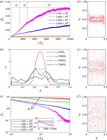
is shown in figure 17(a) for several values of
 $\mathit{Ra}$
. In all cases
 ${\it\sigma}_{Z}^{2}$
increases with time before reaching a plateau. Near the onset of unsteadiness
 $\mathit{Ra}_{c}$
,
 ${\it\sigma}_{Z}^{2}$
remains far from its limit value
 $\max ({\it\sigma}_{Z}^{2})$
in (6.1) even at large times.
Plots of: (a)
 ${\it\sigma}_{Z}^{2}(t)$
for different values of
 $\mathit{Ra}$
(see § 6 for comments about
 $R_{1},R_{2}$
and
 $R_{3}$
); (b)
 ${\it\gamma}(Z,t)$
at four different times at
 $\mathit{Ra}=2.05\times 10^{8}$
; and (c)
 ${\it\sigma}_{{\it\gamma}}^{2}(t)$
for several values of
 $\mathit{Ra}$
. The slope indicated in the figure corresponds to the mixing rate for
 $\mathit{Ra}=2.05\times 10^{8}$
. Inset:
 ${\it\sigma}_{{\it\gamma}}^{2}(t)$
in lin/log scale. Right column: the spreading of particles after (d)
 $250\times T_{0}$
, (e)
 $2800\times T_{0}$
and (f)
 $7000\times T_{0}$
for
 $\mathit{Ra}=2.5\times 10^{8}$
.

We focus now on the largest value
 $\mathit{Ra}=2.05\times 10^{8}$
considered in this study. Three different consecutive stages
 $R_{1}$
,
 $R_{2}$
and
 $R_{3}$
can be identified in figure 17(a). Here
 $R_{1}$
and
 $R_{2}$
both show linear dependence on time yet with different growth rates, while
 $R_{3}$
corresponds to the transient regime preceding a plateau now very close to
 $\max ({\it\sigma}_{Z}^{2})$
. Even if tracers are discrete entities and their number is finite, it is possible to define a pseudo-concentration and study its dependence on time. The pseudo-concentration
 ${\it\gamma}$
is chosen to depend on the spatial variable
 $Z$
only, the
 $X$
-dependence being averaged out by construction. The cavity is first split along the
 $Z$
-axis into
 $m$
segments
 $I_{1},I_{2},\dots ,I_{m}$
of equal vertical extent
 $1/m$
. If each segment
 $I_{j}$
contains exactly
 $M_{j}$
tracers at time
 $t$
, and
 $Z$
belongs to a given segment
 $I_{i}$
, the pseudo-concentration
 ${\it\gamma}(Z,t)$
is later defined as
 $$\begin{eqnarray}{\it\gamma}(Z,t)=\frac{M_{i}}{\displaystyle \frac{1}{m}\mathop{\sum }\limits_{j=1}^{m}M_{j}}\end{eqnarray}$$
In the extreme case of a perfectly homogeneous distribution of tracers,
 ${\it\gamma}=1$
everywhere and its spatial variance
 ${\it\sigma}_{{\it\gamma}}^{2}$
is zero. The time evolution of
 ${\it\gamma}(Z)$
is shown in figure 17(b) using
 $m=20$
. At early times, particles are concentrated around the mid-height of the cavity, close to the tangles associated with
 ${\it\Gamma}_{2,1}$
and
 ${\it\Gamma}_{2,2}$
. As time increases, tracers migrate from the centre towards the rest of the cavity (see figure 17
d–f). Figure 17(b) allows for an interpretation of the stages
 $R_{1}$
,
 $R_{2}$
and
 $R_{3}$
identified in figure 17(a). Here
 $R_{1}$
corresponds to tracers progressively invading the region
 $Z\in [0.3,0.7]$
, i.e. the remains of regions
 $A_{3}$
and
 $N_{2}$
defined for a smaller value of
 $\mathit{Ra}$
. The dynamics associated with
 $R_{1}$
scales as
 ${\it\sigma}_{Z}^{2}\approx 3.1\times 10^{-3}t$
. Here
 $R_{2}$
in turn corresponds to tracers invading the outward regions
 $Z\in [0,0.3]$
and
 $Z\in [0.7,1]$
, with
 ${\it\sigma}_{Z}^{2}\approx 4.7\times 10^{-3}t$
. Here
 $R_{2}$
approximatively corresponds to regions
 $A_{2}$
,
 $N_{1}$
and
 $A_{1}$
in figure 6. The relative acceleration undergone by
 ${\it\sigma}_{Z}^{2}$
between
 $R_{1}$
and
 $R_{2}$
is consistent with the different dynamics identified at lower
 $\mathit{Ra}$
in the previous section. In particular,
 $N_{2}$
is known to result from the break-up and overlapping of an infinity of chains of non-mixing islands. These structures are expected to increase statistically the stickiness of tracers and hence to slow down the spreading process. The linear scaling of the variance in
 $R_{1}$
and
 $R_{2}$
expresses the diffusive motion of tracers in those regions (Cencini et al.
Reference Cencini, Cecconi and Vulpiani2010). At the end of the stage
 $R_{2}$
the tracers have spread by
 $t\approx 2800$
throughout the whole cavity while their distribution is still far from homogeneous, as indicated by the still large values of
 ${\it\sigma}_{{\it\gamma}}^{2}$
. The last stage
 $R_{3}$
consists in a slow homogenisation of the concentration along the
 $Z$
-axis.
We investigate now the speed at which the homogenisation process takes place. For larger times, the variance
 ${\it\sigma}_{{\it\gamma}}^{2}=\langle ({\it\gamma}-\langle {\it\gamma}\rangle _{Z})^{2}\rangle _{Z}$
is expected to tend to zero when the system tends to homogeneity. This limit cannot be reached as long as non-mixing islands persist in the system. For a hyperbolically mixing system,
 ${\it\sigma}_{{\it\gamma}}^{2}\approx \text{e}^{-{\it\alpha}t}$
asymptotically in time, while for a non-hyperbolic one
 ${\it\sigma}_{{\it\gamma}}^{2}\approx t^{-{\it\lambda}}$
where
 ${\it\lambda}$
corresponds to the algebraic mixing rate of the system. The present simulations, carried over
 $10^{4}$
periods, demonstrate a decrease of
 ${\it\sigma}_{{\it\gamma}}^{2}$
by two decades only, which however is enough to exhibit an algebraic decay. The algebraic mixing rate is estimated as
 ${\it\lambda}=2.276$
for
 $\mathit{Ra}=2.05\times 10^{8}$
. No algebraic decay rate could be extracted satisfactorily from simulations at lower values of
 $\mathit{Ra}$
, where mixing can definitely not be considered as complete even in a loose sense. The reasons explaining the algebraic decay for
 $\mathit{Ra}=2.05\times 10^{8}$
have been already discussed earlier and are two-fold: (i) a few small non-mixing islands are still present in the system and induce stickiness of the trajectories in their neighbourhood; (ii) the walls act as non-hyperbolic streamlines. The fact that even a region of negligible area can radically alter the long-time asymptotical decay of the concentration variance is typical of area-preserving systems (see e.g. Artuso Reference Artuso1999) and has been recently demonstrated theoretically (Salman & Haynes Reference Salman and Haynes2007) and experimentally in high-Schmidt-number fluid mixtures (Gouillart et al.
Reference Gouillart, Dauchot, Dubrulle, Roux and Thiffeault2008).
As an important conclusion of the present section, mixing is almost complete before the periodic regime bifurcates towards quasiperiodic dynamics. This suggests that it is not necessary to consider dynamics more complex than the time-periodic regime to achieve complete mixing in this two-dimensional cavity flow.
7. Summary and conclusions
We have investigated numerically the mixing of passive tracers for infinite Schmidt number in a closed two-dimensional differentially heated cavity. This flow is chosen as a prototype of closed convection flow in which several fundamental ideas can be tested, while it is also a widespread geometrical configuration in thermal engineering. It is demonstrated here that the first Hopf bifurcation of the Eulerian system with increasing Rayleigh number coincides with the onset of Lagrangian mixing in the cavity, and that the transition to almost-complete mixing takes place before the Eulerian system bifurcates into the quasi-periodic regime. Only the central region of the cavity appears in finite-time computations as robustly non-mixing because of the almost-vanishing velocities implied by the central symmetry of the flow field. It is hence interpreted as the dead zone of the flow. Using a scattering approach borrowed from studies of mixing in open flows, it is suggested that the flow in the partial mixing regime can be split into several zones characterised by different return-time statistics. The statistics suggest the existence of both hyperbolic and non-hyperbolic regions. The latter result from the persistence of KAM tori as well as from the no-slip conditions at the walls. If the presence of the non-mixing islands gradually reduces with increasing
 $\mathit{Ra}$
, the effect of the walls is weakly dependent on the value of
 $\mathit{Ra}$
and should manifest itself in all regimes from laminar to fully turbulent. The extraction of a large number of UPOs of the Lagrangian system (3.1) allows one for visualising the tangles resulting from intersecting bundles of manifolds (Feudel et al.
Reference Feudel, Witt, Gellert, Kurths, Gregobi and Sanjuán2005), i.e. the mixing regions. The elliptic periodic orbits indicate the proximity of non-mixing islands. Such orbits are associated with streamlines of the base flow in resonance with the oscillatory global mode. Superimposing all of the corresponding manifolds in forward and backward time leads to a visualisation as well as to a multiscale quantification of the fraction of chaos in the system. Non-hyperbolicity governs global statistics such as the temporal decay of the concentration variance at higher values of
 $\mathit{Ra}$
. This result is classical in the literature on Hamiltonian systems. Our measurement of the algebraic mixing rate is here based on brute force computations and on the definition of a coarse-grained pseudo-concentration field. Refined alternative methods have been suggested recently to compute the algebraic mixing rate directly from the knowledge of the statistics of finite-time Lyapunov exponents (Artuso & Manchein Reference Artuso and Manchein2009). Such methods are attractive given the recent attention on Lagrangian coherent structures precisely based on the computation of finite-time Lyapunov exponents, yet they remain to be tested in this context.
A natural question is the extension of the present results to the case of diffusive tracers, as e.g. dye in an experimental set-up. The addition of a Gaussian white noise to (3.1) is strictly equivalent to the addition of a molecular diffusivity for the tracers, i.e. to a finite Schmidt number. In that case the algebraic decay of the statistics would be lost in favour of a classical exponential decay (see e.g. Pikovsky & Popovych Reference Pikovsky and Popovych2003). It is however expected that the topology of the flow, in particular the location of homoclinic and heteroclinic loops, would still govern the dynamics of the tracers over very long times, at least in the weakly diffusive limit.
There are several ways to extend the present two-dimensional configuration to three dimensions. The differentially heated cavity flow has been the subject of a few three-dimensional Eulerian investigations, but so far only by considering confinement or extension in the third direction. For the extended case, it was shown that the first bifurcations from the base state involve very slow travelling waves located in the near-wall regions (Xin & Le Quéré Reference Xin and Le Quéré2012). In a given transverse section, the two-dimensional base flow can be seen as modulated by the passage of the wave. Although the system is no longer Hamiltonian it is expected that the mixing phenomenology, based on tori resonances and on the presence of homoclinic tangles, would be qualitatively analogous to the unsteady two-dimensional case investigated here. Other interesting generalisations to three dimensions are perturbed axisymmetric geometries in which the two-dimensional set-up is recovered approximatively in each meridional section. When the unperturbed flow possesses a component along the invariant azimuthal direction
 ${\it\theta}$
, the Lagrangian system has a Hamiltonian structure, and the occurrence of KAM tori as transport barriers was demonstrated in a Poincaré section
 ${\it\theta}=cst$
(Fountain et al.
Reference Fountain, Khakhar, Mezic and Ottino2000; Pratta et al.
Reference Pratta, Rypina, Özgökmen, Wang, Childs and Bebieva2014). Steady states in a cubic geometry have been investigated by Tric, Labrosse & Betrouni (Reference Tric, Labrosse and Betrouni2000). For such genuinely three-dimensional flows there is no straightforward methodology based on the knowledge of continuous symmetries in order to identify barriers to mixing. We expect however that the influence of the walls on the mixing rate is analogous to the two-dimensional case.
Acknowledgements
We would like to thank Airbus Group (EADS Foundation) for its financial support, as well as S. Xin for sharing his DNS code.
Appendix. A fast algorithm to locate periodic points
We describe here a simple and original algorithm used to identify fixed points or periodic points in the two-dimensional stroboscopic section
 ${\it\Pi}$
. The algorithm is inspired by the secant method. Its convergence properties have proven comparable or faster than the alternative Newton–Raphson solver in the present case. The algorithm identifies iteratively a zero of
 $\boldsymbol{g}={\bf\pi}^{n}-\boldsymbol{I}$
for a given integer
 $n>0$
by a simple bisection procedure. It is structured as follows.
-
(a) Select an initial candidate
$\boldsymbol{X}_{0}$
. -
(b) Consider the square of side
$2d$
centred on
$\boldsymbol{X}_{0}$
with sides parallel to
$X$
and
$Z$
. Label by
$\boldsymbol{X}_{i}$
,
$i=1,\dots ,8$
the corners of the square and the middle of each side. -
(c) Evaluate the displacement
$\boldsymbol{g}_{\boldsymbol{i}}=\boldsymbol{g}(\boldsymbol{X}_{i})$
at all points
$\boldsymbol{X}_{i}$
,
$i=0,\dots ,8$
. -
(d) Select among them the point
$\boldsymbol{X}_{k}$
for which all components of
$\boldsymbol{g}_{\boldsymbol{k}}$
have opposite sign compared with
$\boldsymbol{g}_{0}$
and for which
$|\boldsymbol{g}_{\boldsymbol{k}}|^{2}$
is minimal. If such a point does not exist, simply select the point where
$|\boldsymbol{g}(\boldsymbol{X}_{k})|^{2}$
is minimal, set
$\boldsymbol{X}_{b}=(\boldsymbol{X}_{k}+\boldsymbol{X}_{0})/2$
,
$\boldsymbol{X}_{0}=\boldsymbol{X}_{b}$
and go back to step (b). -
(e) Define the new candidate
$\boldsymbol{X}_{b}=(\boldsymbol{X}_{k}+\boldsymbol{X}_{0})/2$
. -
(f) If
$|\boldsymbol{g}(\boldsymbol{X}_{b})|<10^{-10}$
a fixed/periodic point has been identified. Otherwise: -
(g) Update
$d=\Vert \boldsymbol{X}_{b}-\boldsymbol{X}_{0}\Vert _{\infty }$
,
$\boldsymbol{X}_{0}=\boldsymbol{X}_{b}$
and go back to step (b).