


1. Introduction
Magnetic helicity  ${{\mathcal {H}}^M}=\langle {\boldsymbol {a}} \cdot {\boldsymbol {b}} \rangle$, defined as the helicity of the magnetic vector potential
 ${\boldsymbol {a}}$ (so that
 ${\boldsymbol {b}}=\boldsymbol {\nabla } \times {\boldsymbol {a}}$ is the magnetic field), with
 $\langle \cdot \rangle$ denoting the volume average, is a quantity expressing topological aspects of the magnetic field lines, such as their degree of linkage, twist, writhe and knottedness (Moffatt Reference Moffatt1969). In a closed volume with a vanishing magnetic field component normal to the volume boundaries, or a periodic domain without mean magnetic field, magnetic helicity is gauge invariant (Biskamp Reference Biskamp1993; Berger Reference Berger1997). In space, because of the very low resistivity, magnetic field lines are effectively ‘frozen-in’ the ionised gas (plasma) present in various degrees of ionisation throughout the universe (Alfvén Reference Alfvén1942). As a consequence, rotational motion is expected to naturally generate helical magnetic fields. Since magnetic helicity is an ideal invariant of the magnetohydrodynamic (MHD) equations (Elsässer Reference Elsässer1956; Woltjer Reference Woltjer1958), it can be an important constraint on the time evolution of magnetic fields, which plays a crucial role in many astrophysical systems of interest. For example, magnetic helicity dynamics are involved in solar flares and coronal mass ejections (Low Reference Low1994), which transfer magnetic helicity from the Sun to the interplanetary medium (Kumar & Rust Reference Kumar and Rust1996). The Sun also emits magnetic helicity through the solar wind (Bieber, Evenson & Matthaeus Reference Bieber, Evenson and Matthaeus1987), which is manifested at the largest scales through the Parker spiral (Berger Reference Berger1999). Magnetic helicity conservation is also very important in dynamo processes (Brandenburg Reference Brandenburg2001; Vishniac & Cho Reference Vishniac and Cho2001; Brandenburg & Lazarian Reference Brandenburg and Lazarian2013). In laboratory plasmas, it is of relevance for plasma confinement in reversed-field pinch fusion experiments (Escande et al. Reference Escande2000).
Magnetic helicity is subject to an inverse transfer in spectral space, as has been suggested in Frisch et al. (Reference Frisch, Pouquet, Léorat and Mazure1975) and subsequently confirmed by various numerical experiments (Pouquet, Frisch & Léorat Reference Pouquet, Frisch and Léorat1976; Pouquet & Patterson Reference Pouquet and Patterson1978; Meneguzzi, Frisch & Pouquet Reference Meneguzzi, Frisch and Pouquet1981; Balsara & Pouquet Reference Balsara and Pouquet1999; Brandenburg Reference Brandenburg2001; Christensson & Hindmarsh Reference Christensson, Hindmarsh and Brandenburg2001; Alexakis, Mininni & Pouquet Reference Alexakis, Mininni and Pouquet2006; Malapaka Reference Malapaka2009; Müller, Malapaka & Busse Reference Müller, Malapaka and Busse2012; Linkmann & Dallas Reference Linkmann and Dallas2016; Linkmann et al. Reference Linkmann, Sahoo, McKay, Berera and Biferale2017). This key property renders magnetic helicity a potentially important quantity in the generation and sustainment of large-scale magnetic fields in the universe. In direct numerical simulations of astrophysical plasma, the achievable Reynolds numbers are far below the ones expected in nature. A possibility for tackling this issue is to use large-eddy simulations (known as LES) with underlying subgrid-scale models, which are often constructed considering only the direct energy cascade. Understanding better the magnetic helicity dynamics is hence of great importance for the development of more realistic large-eddy simulations subgrid models (Miesch et al. Reference Miesch2015).
Up to the present day, the inverse transfer of magnetic helicity in single-fluid MHD has been studied assuming either an incompressible plasma (Alexakis et al. Reference Alexakis, Mininni and Pouquet2006; Malapaka Reference Malapaka2009; Müller et al. Reference Müller, Malapaka and Busse2012), or in the subsonic/transonic case (Balsara & Pouquet Reference Balsara and Pouquet1999; Brandenburg Reference Brandenburg2001; Christensson & Hindmarsh Reference Christensson, Hindmarsh and Brandenburg2001). Detailed studies on the properties of the transfer of energy and helicity, in particular its spectral locality, have also been carried out by Aluie (Reference Aluie2017), Alexakis et al. (Reference Alexakis, Mininni and Pouquet2006), Alexakis & Biferale (Reference Alexakis and Biferale2018) and Linkmann & Dallas (Reference Linkmann and Dallas2016). In astrophysical systems, however, flows are often highly supersonic. For example, the order of magnitude of the root mean square (RMS) turbulent Mach number ranges from 0.1 to approximately 10 in the interstellar medium (Elmegreen & Scalo Reference Elmegreen and Scalo2004, § 4.2). The present work makes one step towards a more realistic setting by including compressible effects in the framework of supersonic isothermal ideal MHD. The inverse transfer of magnetic helicity is investigated through direct numerical simulations of large-scale mechanically driven compressible plasma under the continuous injection of small-scale random helical magnetic fluctuations. The large-scale mechanical forcing is either purely solenoidal or purely compressive and the considered RMS Mach numbers of the initial hydrodynamic turbulent statistically stationary states range from 0.1 to 11 for solenoidal driving, and from 1 to 8 for compressive driving.
A similar numerical set-up in the incompressible case, where magnetic helical fluctuations are injected at small scales in the absence of a large-scale mechanical forcing has shown that several quantities, including the kinetic and magnetic energies and helicities, exhibit approximate power-law scaling in Fourier space in the inverse transfer region, i.e. at spatial scales larger than those of the magnetic driving (Malapaka Reference Malapaka2009; Müller et al. Reference Müller, Malapaka and Busse2012). Furthermore, a dynamic balance leading to a quasi-equipartition between magnetic and kinetic energies on the one hand, and current and kinetic helicities on the other hand, has been observed in several numerical experiments in the incompressible case (Malapaka Reference Malapaka2009; Mininni & Pouquet Reference Mininni and Pouquet2009; Graham, Mininni & Pouquet Reference Graham, Mininni and Pouquet2011; Müller et al. Reference Müller, Malapaka and Busse2012). The purpose of the present work is to investigate similarities and differences in the spectral scaling laws, and this dynamic balance for turbulent flows exhibiting significant compressible effects. The scaling properties are expected to change, since in compressible MHD the magnetic field time evolution is governed by
 \begin{equation} \partial_t {\boldsymbol{b}} ={-}({\boldsymbol{v}} \boldsymbol{\cdot} \boldsymbol{\nabla}) {\boldsymbol{b}}+({\boldsymbol{b}} \boldsymbol{\cdot} \boldsymbol{\nabla}) {\boldsymbol{v}} - {\boldsymbol{b}} (\boldsymbol{\nabla} \boldsymbol{\cdot} {\boldsymbol{v}}). \end{equation}
For a high level of compression, the magnetic field and hence magnetic helicity dynamics are expected to be affected through two aspects. First, through the compression term  $-{\boldsymbol {b}} (\boldsymbol {\nabla } \boldsymbol {\cdot } {\boldsymbol {v}})$, which is not present in incompressible MHD. Second, even though the advective
 $-({\boldsymbol {v}} \boldsymbol {\cdot } \boldsymbol {\nabla }){\boldsymbol {b}}$ and the stretching
 $({\boldsymbol {b}} \boldsymbol {\cdot } \boldsymbol {\nabla }){\boldsymbol {v}}$ terms are also present in the incompressible case, the velocity field's compressive part may alter them. An analysis of the influence of the compressive velocity field on these three terms is the object of a forthcoming work.
The numerical method used, as well as the simulation set-up, are described in § 2. Section 3 summarises some findings of previous research, which are put in relation with this work's results in § 4. Finally, § 5 assesses the robustness of the results while concluding remarks are given in § 6.
2. Numerical experiments
2.1. MHD numerical solver
The isothermal ideal (single fluid) MHD equations, in the presence of both a mechanical and an electromotive forcing, can be written as
 \begin{gather} \partial_t \rho ={-} \boldsymbol{\nabla}\boldsymbol{\cdot} (\rho {\boldsymbol{v}}), \end{gather}
 \begin{gather}\partial_t (\rho {\boldsymbol{v}}) ={-} \boldsymbol{\nabla} \boldsymbol{\cdot} ( \rho {\boldsymbol{v}} {\boldsymbol{v}}^{\textrm{T}} + (\rho c_s^2 + \tfrac{1}{2}|{\boldsymbol{b}}|^2){\boldsymbol{\mathsf{I}}} - {\boldsymbol{b}} {\boldsymbol{b}}^{\textrm{T}} )+\rho\boldsymbol{f}_V, \end{gather}
 \begin{gather}\partial_t {\boldsymbol{b}} = \boldsymbol{\nabla} \times ({\boldsymbol{v}} \times {\boldsymbol{b}})+\boldsymbol{f}_M, \end{gather}
 \begin{gather}\boldsymbol{\nabla}\boldsymbol{\cdot} {\boldsymbol{b}}=0, \end{gather}
with  $\rho$ the mass density,
 ${\boldsymbol {v}}$ the fluid velocity,
 $c_s$ the constant isothermal sound speed so that
 $p=\rho c_s^2$ is the (thermal) pressure and
 ${\boldsymbol {b}}$ the magnetic field so that
 $\boldsymbol {E}=-{\boldsymbol {v}} \times {\boldsymbol {b}}$ is the electric field. The
 $3\times 3$ identity matrix is denoted by
 ${\boldsymbol{\mathsf{I}}}$. The mechanical driving occurs through an acceleration field (
 $\boldsymbol {f}_V$) and the magnetic helical fluctuations are injected through an electromotive forcing (
 $\boldsymbol {f}_M$). These two terms are described in § 2.2.
The numerical solver is a shock-capturing fourth-order finite volume method, described in detail in Teissier (Reference Teissier2020) and Verma et al. (Reference Verma, Teissier, Henze and Müller2019). The main reconstruction method used is a fourth-order central weighted essentially non-oscillatory (known as CWENO) procedure (Levy, Puppo & Russo Reference Levy, Puppo and Russo1999), with a passage through point values in order to maintain the fourth-order accuracy (McCorquodale & Colella Reference McCorquodale and Colella2011; Buchmüller & Helzel Reference Buchmüller and Helzel2014). The interfacial fluxes are computed using the Rusanov approximation (Rusanov Reference Rusanov1961), also known as ‘local Lax–Friedrichs’. In order to prevent the appearance of negative densities in high-Mach-number flows, a local reduction of the reconstruction order in the vicinity of strong discontinuities and shocks is used (an approach often referred to as a ‘flattening’ or ‘fallback approach’ (Colella & Woodward Reference Colella and Woodward1984; Balsara Reference Balsara2012; Núñez-de la Rosa & Munz Reference Núñez-de la Rosa and Munz2016)). This has the effect of adding some numerical dissipation locally, which smoothens the solution and also prevents oscillations of high-order polynomials on regular grids. The magnetic field solenoidality is maintained up to machine precision by application of the constrained transport approach (Evans & Hawley Reference Evans and Hawley1988), making use of a multidimensional version of the Rusanov flux to compute the line-integrated electric field (Balsara Reference Balsara2010). The time integration is implemented as a fourth-order 10-stages strong-stability-preserving Runge–Kutta (known as SSPRK) method (Ketcheson (Reference Ketcheson2008), pseudocode 3). The discrete time step  $\Delta t$ is constrained by the Courant–Friedrichs–Lewy criterion with a Courant number of
 $C_{CFL}=1.5$.
2.2. Simulation and diagnostics procedure
The power spectrum  ${\mathcal {P}}(\,\boldsymbol {{f}})$ of a field
 $\boldsymbol {{f}}$ shown in this work is defined by a summation over each wavenumber shell
 $K \in \mathbb {N}$. A shell consists of all the wavevectors
 $\boldsymbol {k}$ such that
 $K \leq |\boldsymbol {k}|/\kappa < K+1$ with
 $\kappa =2{\rm \pi} /L$ the smallest wavenumber in the system, giving the spectrum
 \begin{equation} {\mathcal{P}}(\,\boldsymbol {{f}})_K=\tfrac{1}{2} \sum_{K \leq |\boldsymbol{k}|/\kappa < K+1} |\,\boldsymbol{\hat {f}}_{\boldsymbol{k}}|^2, \end{equation}
with  $\boldsymbol {\hat {f}}_{\boldsymbol {k}}$ the Fourier coefficient at wavevector
 $\boldsymbol {k}$. The compressive part of a power spectrum,
 ${\mathcal {P}}^{comp}(\,\boldsymbol {{f}})$, considers only the contributions parallel to the wavevector
 \begin{equation} {\mathcal{P}}^{comp}(\,\boldsymbol {{f}})_K=\tfrac{1}{2}\sum_{K \leq |\boldsymbol{k}|/\kappa < K+1} |\,\boldsymbol{\hat {f}}_{\boldsymbol{k}} \cdot \boldsymbol{k}|^2/|\boldsymbol{k}|^2. \end{equation}
The solenoidal part of a power spectrum is built accordingly through the difference  ${\mathcal {P}}^{sol}(\,\boldsymbol {{f}})={\mathcal {P}}(\,\boldsymbol {{f}})-{\mathcal {P}}^{comp}(\,\boldsymbol {{f}})$.
The considered turbulent systems exhibit both a direct cascade of kinetic energy from large to small scales and an inverse transfer of magnetic helicity, from small to large scales. The terminology ‘cascade’ is not used here for the magnetic helicity inverse transfer, since this process displays pronounced spectrally non-local features (Alexakis et al. Reference Alexakis, Mininni and Pouquet2006; Linkmann & Dallas Reference Linkmann and Dallas2016; Teissier Reference Teissier2020). The statistically stationary turbulent state is generated and sustained through a continuous large-scale mechanical driving in a triply periodic cubic simulation domain with linear size  $L=1$. The isothermal sound speed is taken as
 $c_s=0.1$. Starting with a constant-density plasma at rest (
 $\rho =\rho_0=1, {\boldsymbol {v}}=0,{\boldsymbol {b}}=0$), an Ornstein–Uhlenbeck driving injects kinetic energy at large scales, similar to Federrath et al. (Reference Federrath, Roman-Duval, Klessen, Schmidt and Mac Low2010) and Federrath (Reference Federrath2013). It is defined, starting with
 $\boldsymbol { F^{OU}_{\boldsymbol {k}}}=0$, by the following stochastic differential equation in Fourier space:
 \begin{equation} \textrm{d}\boldsymbol{ F^{OU}_{\boldsymbol{k}}}(t)={-}\boldsymbol{ F^{OU}_{\boldsymbol{k}}}(t)\frac{\textrm{d} t}{t_{auto}}+F_0 \left( \frac{2\sigma(\boldsymbol{k})^2}{t_{auto}} \right)^{1/2} \underline{{\mathcal{P}^{\zeta}}} \cdot \textrm{d}\boldsymbol{W}(t), \end{equation}
with  $t_{auto}=L/(2c_s{\mathcal {M}}^{*})$ the forcing autocorrelation time, where
 ${\mathcal {M}}^*$ is an a priori estimate of the expected RMS Mach number during the statistically stationary state,
 $F_0$ an amplitude,
 $\sigma$ a spectral profile,
 $\textrm {d}\boldsymbol {W}(t)=\textrm {d} t\boldsymbol {N}(0,\textrm {d} t)$ a Wiener process with
 $\boldsymbol {N}(0,\textrm {d} t)$ a three-dimensional Gaussian distribution with zero mean and standard deviation
 $dt$ representing a three-dimensional continuous random walk. The projection operator
 ${{\mathcal {P}}^{\zeta }_{ij}}(\boldsymbol {k})=\zeta \delta _{ij}+(1-2\zeta ) ({k_ik_j}/{|k|^2})$ allows us to control the forcing's compressivity: for
 $\zeta =0$, only components along
 $\boldsymbol {k}$ are kept so that the forcing is purely compressive, whereas for
 $\zeta =1$, the forcing is projected on the plane orthogonal to
 $\boldsymbol {k}$ in Fourier space and the resulting field is purely solenoidal. The spectral profile is taken as
 $\sigma (\boldsymbol {k})=1$ for the wavenumber shells
 $1 \leq K \leq 2$ and 0 otherwise, so that only the largest scales are forced.
The mechanical forcing is applied after the 10 stages of the strong-stability-preserving Runge–Kutta integration method, through
 \begin{equation} (\rho {\boldsymbol{v}}) \leftarrow (\rho {\boldsymbol{v}})+\rho \Delta t \boldsymbol{f}_V, \end{equation}
with  $\boldsymbol {f}_V=A_V \tilde {\boldsymbol {f}}_V$, where
 $\tilde {\boldsymbol {f}}_V$ is the
 $\boldsymbol {F^{OU}}$ field in configuration space, multiplied by an amplitude
 $A_V$. This amplitude is introduced in order to guarantee a constant energy injection rate
 ${\epsilon ^{K}_{inj}}={\rm \Delta} {\mathcal {E}}^K/\Delta t$ and is determined by the largest root of the second-order equation (cf. Mac Low Reference Mac Low1999)
 \begin{equation} {\rm \Delta} {\mathcal{E}}^K =\tfrac{1}{2} A_V^2 \Delta t^2 \sum_{i,j,k} \rho_{i,j,k} \,\tilde{\boldsymbol{f}}_{V,i,j,k}^2+A_V\Delta t \sum_{i,j,k} \rho_{i,j,k} {\boldsymbol{v}}_{i,j,k} \cdot \tilde{\boldsymbol{f}}_{V,i,j,k}, \end{equation}
where  $q_{i,j,k}$ designates the value of field
 $q$ in the numerical cell indexed by
 $(i,j,k)$. As a consequence of this normalisation, the choice of the constant amplitude
 $F_0$ in relation (2.7) is arbitrary. The injected energy cascades to ever smaller scales where it is finally dissipated due to numerical non-ideal effects, which serve as a simple model for physical viscosity and resistivity. Thus, a statistically stationary state is reached with a roughly constant RMS Mach number
 ${\mathcal {M}} = \sqrt { \langle |{\boldsymbol {v}}|^2/c_s^2 \rangle } \approx {\mathcal {M}}^*$ on a time scale of the order of the turbulent turnover-time
 $t_{\mathcal {T}}=L/(2c_s{\mathcal {M}})$ (Federrath Reference Federrath2013). Hence the forcing autocorrelation time
 $t_{auto}$ is taken close to the turbulent large-eddy turnover time, the natural time of propagation of information from the largest to the smallest scales in the turbulent flow. The energy injection rate determines the RMS Mach number,
 ${\mathcal {M}}$, of the statistically stationary state. The weak fluctuating mean velocity field which appears as a result of the driving is removed at each iteration. Only the strict conservation of momentum (and energy) are guaranteed up to machine precision by the numerical scheme – this does not prevent the secular generation of a finite mean velocity component by the statistical process that represents the turbulence driver. The removal of a mean velocity is important in the presence of magnetic fields which break the Galilean invariance of the system. At a particular instant in time during the turbulent hydrodynamic statistically stationary state, a small-scale electromotive helical driving is switched on while maintaining the large-scale mechanical driving. The electromotive forcing injects delta-correlated (white noise) maximally helical magnetic fluctuations at the wavenumber shells
 $48 \leq K \leq 52$ and is defined in Fourier space by
 \begin{equation} \boldsymbol{F^M_{\boldsymbol{k}}}=B_{\boldsymbol{k}}^+ \,\textrm{e}^{\textrm{i}\theta_{\boldsymbol{k}}^+}\boldsymbol{{{\hat{h}}}^{+}_{\boldsymbol{k}}}, \end{equation}
with  $\theta _{\boldsymbol {k}}^+$ a random phase chosen uniformly in
 $[0,2{\rm \pi} ]$ and
 $\boldsymbol {{{\hat {h}}}^{+}_{\boldsymbol {k}}}$ an eigenvector of the curl operator such that
 $\textrm {i}\boldsymbol {k} \times \boldsymbol {{{\hat {h}}}^{+}_{\boldsymbol {k}}}=+|\boldsymbol {k}| \boldsymbol {{{\hat {h}}}^{+}_{\boldsymbol {k}}}$. The curl operator is indeed diagonalisable in Fourier space when using a ‘helical basis’
 $(\boldsymbol {{{\hat {h}}}^{+}_{\boldsymbol {k}}},\boldsymbol {{{\hat {h}}}^{-}_{\boldsymbol {k}}})$ with
 $\textrm {i}\boldsymbol {k} \times \boldsymbol {{{\hat {h}}}^{\pm }_{\boldsymbol {k}}}=\pm |\boldsymbol {k}|\boldsymbol {{{\hat {h}}}^{\pm }_{\boldsymbol {k}}}$ (see e.g. Waleffe (Reference Waleffe1992) and Brandenburg & Subramanian (Reference Brandenburg and Subramanian2005)). In this way, the electromotive driving is chosen as maximally helical (positive sign). The amplitude
 $B_{\boldsymbol {k}}^+$ in the different shells is given by
 \begin{equation} B_{\boldsymbol{k}}^+{=}\exp\left[\frac{1}{2}\left(\frac{|\boldsymbol{k}|/\kappa-K_H}{4}\right)^2\right], \end{equation}
with  $K_H=50$ the shell around which the electromotive driving takes place. Similarly to the mechanical forcing, the resulting field in configuration space,
 $\tilde {\boldsymbol {f}}_M$, is applied after the 10 stages of the time integration procedure. It is renormalised in a way analogous to
 $\tilde {\boldsymbol {f}}_V$ in order to guarantee a constant magnetic energy injection rate
 ${\epsilon ^{M}_{inj}}={\rm \Delta} {\mathcal {E}}^M/\Delta t$.
The mechanical forcing and the electromotive driving occur at different spatial scales in order to observe the effects of compressibility. Indeed, compressibility effects enter the magnetic helicity dynamics via a term  $\sim \boldsymbol {\nabla } \boldsymbol {\cdot } {\boldsymbol {v}}$, so that if both
 ${\boldsymbol {v}}$ and
 ${\boldsymbol {b}}$ would be driven at small scales (as in Müller et al. (Reference Müller, Malapaka and Busse2012)), the velocity field at scales larger than the driving, excited solely by an inverse transfer of the magnetic field, would be far too weak to have observable effects.
Regarding the spectral diagnostics, the helicity spectra are defined as the cospectrum of a field  $\boldsymbol {{f}}$ and its curl
 $\boldsymbol {{g}}=\boldsymbol {\nabla }\times \boldsymbol {{f}}$ as follows:
 \begin{equation} {\mathcal{Q}}(\,\boldsymbol{{f}},\boldsymbol{{g}})_K=\sum_{K \leq |\boldsymbol{k}|/\kappa < K+1} \boldsymbol{\hat {f}}_{\boldsymbol{k}} \cdot \boldsymbol{\hat {g}}_{\boldsymbol{k}}^*, \end{equation}
with the asterisk  $(^*)$ designating the complex conjugate, so that
 ${\mathcal {P}}(\,\boldsymbol {{f}})=\frac {1}{2}{\mathcal {Q}}(\,\boldsymbol {{f}},\boldsymbol {{f}})$. The magnetic vector potential is computed through the Coulomb gauge
 $\boldsymbol {\nabla }\boldsymbol {\cdot } {\boldsymbol {a}}=0$ so that
 $\boldsymbol {\hat {a}}_{\boldsymbol {k}}=i \boldsymbol {k} \times \boldsymbol {{{}\hat {b}}}_{\boldsymbol {k}}/k^2$ in Fourier space. Expressed in the helical basis, the magnetic helicity spectrum is
 $H^M=H^M_+-H^M_-$ with
 $H^M_{\pm ,\boldsymbol {k}}=|\boldsymbol {{{}\hat {b}}}_{\boldsymbol {k}}\cdot \boldsymbol {{{\hat {h}}}^{\pm ,*}_{\boldsymbol {k}}}|^2/|\boldsymbol {k}|$ the projection of the magnetic field on the positive (respectively, negative) helical eigenvector (Brandenburg & Subramanian Reference Brandenburg and Subramanian2005). The Fourier spectra and cospectra are, furthermore, normalised in order to refer more easily to physical quantities. The power spectrum of the velocity (the specific kinetic energy spectrum) and the kinetic helicity spectrum (cospectrum of velocity and vorticity) are normalised by the isothermal sound speed squared
 $c_s^2$ so that
 ${\mathcal {P}}({\boldsymbol {v}})_K=(1/2)\sum _{K \leq |\boldsymbol {k}|/\kappa < K+1} |\boldsymbol {{{}\hat {v}}}_{\boldsymbol {k}} / c_s|^2$. Similarly, quantities involving the density, such as
 $\boldsymbol {w}=\sqrt {\rho }{\boldsymbol {v}}$, have an additional normalisation by an appropriate power of the mean density
 $\rho _0$. For example,
 ${\mathcal {P}}(\boldsymbol {w})$ is normalised by
 $\rho _0 c_s^2$. Since the mean density is
 $\rho _0=1$, this additional
 $\rho _0$ factor has no direct effect but is still mentioned since the magnetic field
 ${\boldsymbol {b}}$ has the same dimension as
 $\boldsymbol {w}$. For this reason, both the magnetic field power spectrum and the magnetic helicity spectrum are normalised by
 $\rho _0 c_s^2$. These normalisation factors are implicitly assumed in the relations (2.5) and (2.6) and not written explicitly in order to reduce the quantity of notation.
2.3. Simulation runs
The forcing parameters used for the simulated runs and the resulting time-averaged RMS Mach number in the hydrodynamic statistically stationary state  ${\mathcal {M}}$ are displayed in table 1. The number in the runs’ labels stands for their approximate
 ${\mathcal {M}}$ and the letter (‘s’ or ‘c’) for the forcing used (purely solenoidal with
 $\zeta =1$ or purely compressive with
 $\zeta =0$). The main runs are performed at resolution
 $512^3$ and confirmation at higher resolution has been done for selected cases, see § 5. In order to investigate subsonic, transonic and supersonic turbulence at various compressibility,
 ${\mathcal {M}}$ varies in the range
 ${\approx }0.1\text {--}11$ for the solenoidally driven runs and
 ${\approx }1\text {--}8$ for the compressively driven ones. The magnetic-to-kinetic energy injection ratio
 ${\epsilon ^{M}_{inj}}/{\epsilon ^{K}_{inj}}$ is taken as unity for all runs, apart for the M01s4 and M1s2 runs where it is 4 and 2, respectively (as written in the run's label), in order to obtain a faster convergence of the scaling laws in the inverse transfer region. A parameter study in order to assess the influence of the magnetic-to-kinetic energy injection ratio has been performed in Teissier (Reference Teissier2020), § 7.1 and suggests that the approximate scaling exponents observed in the spectral region of inverse transfer converge to the same values as long as
 ${\epsilon ^{M}_{inj}}$ and
 ${\epsilon ^{K}_{inj}}$ are of the same order of magnitude. The rate of convergence increases with a greater magnetic energy injection rate
 ${\epsilon ^{M}_{inj}}$.
Parameters of the simulation: kinetic energy injection rate  ${\epsilon ^{K}_{inj}}$, spectral weight
 $\zeta$ governing the forcing's compressivity, forcing autocorrelation time
 $t_{auto}$, which result in a time-averaged root mean square Mach number
 ${\mathcal {M}}$. During the hydrodynamic statistically stationary state, magnetic helicity injection is switched on with a constant magnetic energy injection rate
 ${\epsilon ^{M}_{inj}}$.

Figure 1 shows mass density slices for the M1s2, M11s, M1c and M8c runs during the hydrodynamic statistically stationary state. Since the mass density is governed by  $\partial _t \rho =-\boldsymbol {\nabla }\boldsymbol {\cdot } (\rho {\boldsymbol {v}})$, a compressive forcing with a high
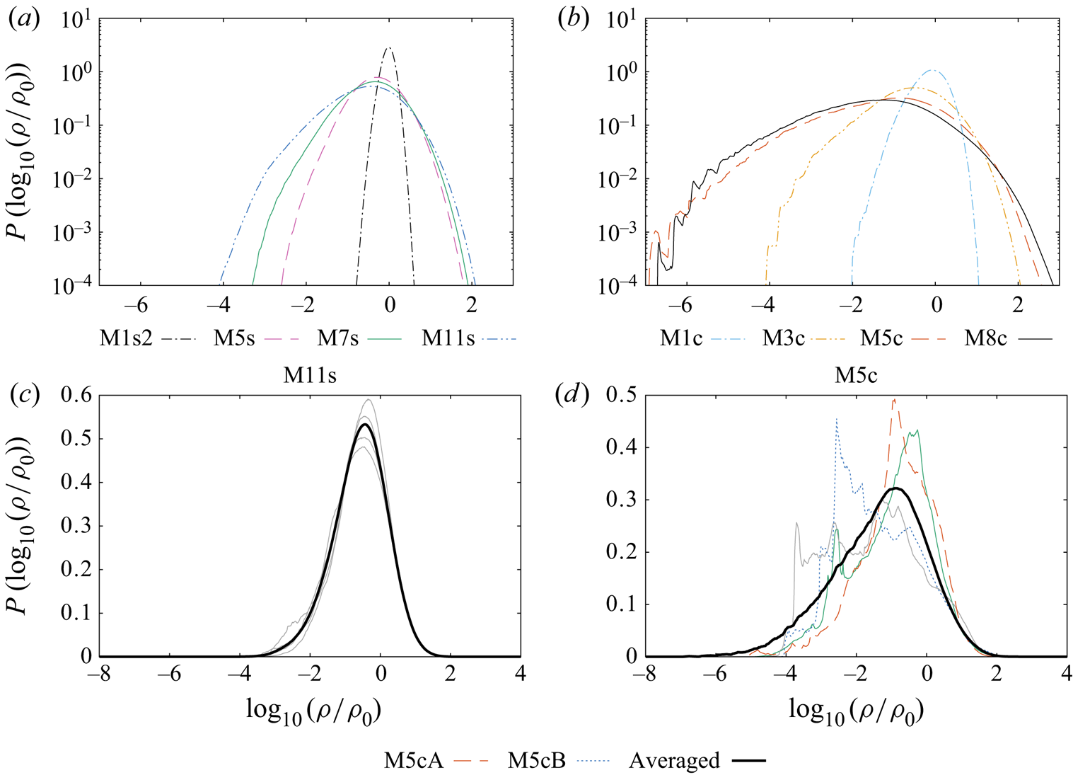
 $\boldsymbol {\nabla }\boldsymbol {\cdot } {\boldsymbol {v}}$ component induces strong mass density variations, visible through regions of very low density for the M8c run and pronounced shock fronts, already present at a RMS Mach number around unity (M1c run). Probability distribution functions (p.d.f.s) of the mass density statistics during the hydrodynamic statistically stationary state are shown in figure 2 and display a considerably larger density spread for compressively driven runs at relatively lower RMS Mach numbers as compared with the solenoidally driven ones: for example, the spread of the M3c run is comparable to the M11s one. These curves are obtained by averaging over at least 40 snapshots equally spaced in time over roughly
 $4t_{\mathcal {T}}$. A sampling rate higher than the turbulent turnover time is chosen because of the high variability of the density p.d.f.s for the supersonic compressively driven runs. For compressively driven turbulence, the snapshot-to-snapshot variations of the density p.d.f.s are significantly greater, as illustrated in figure 2(c,d). For this reason, the influence of the particular snapshot taken as an initial condition for magnetic helicity injection is assessed by taking two different instants in the M5c hydrodynamic statistically stationary state. These runs are hereafter labelled, respectively, ‘M5cA’ and ‘M5cB’ and make use of the initial hydrodynamic state corresponding to the red dashed (respectively, blue dotted) curve in figure 2(d). For all the other runs, only one snapshot in the hydrodynamic statistically stationary state is taken as an initial condition for the magnetic helicity injection.
Mass density slices during the hydrodynamic statistically stationary state for the M1s2, M11s, M1c and M8c runs.

(a,b) Mass density p.d.f. of all transonic and supersonic runs, time-averaged over at least forty  $512^3$ snapshots equally spaced in a time interval of approximately
 $4t_{\mathcal {T}}$. (c,d) Snapshot-to-snapshot variations of the mass density p.d.f.s for the M11s and M5c hydrodynamic statistically stationary state. The thick line corresponds to the time average and the thinner lines to selected snapshots during the statistically stationary state. Among these snapshots, the red dashed and blue dotted curves for the M5c run correspond to different initial conditions for the magnetic helicity injection: the M5cA run's initial condition corresponds to the red dashed curve, whereas the M5cB run's initial condition corresponds to the blue dotted one.

Even though higher-order numerics allow us to see comparatively many details as compared with lower-order schemes, the present simulations also exhibit well known numerical inaccuracies such as, for example, phase and amplitude errors (numerical dissipation, Schmidt, Hillebrandt & Niemeyer (Reference Schmidt, Hillebrandt and Niemeyer2006)), spurious generation of smallest-scale fluctuations (energy excess towards the grid-scale, Falkovich (Reference Falkovich1994); Dobler et al. (Reference Dobler, Haugen, Yousef and Brandenburg2003); Schmidt et al. (Reference Schmidt, Hillebrandt and Niemeyer2006); Federrath (Reference Federrath2013) and Teissier (Reference Teissier2020)) as well as statistical errors due to the finite extent in discretised space and time. Section 5 addresses this issue by testing the robustness of the obtained results.
3. Previous research
An experimental set-up similar to the one presented here has led to the observation of several spectral scaling laws for incompressible MHD turbulence (Malapaka Reference Malapaka2009; Müller et al. Reference Müller, Malapaka and Busse2012). In these works, pseudo-spectral direct numerical simulations with  $1024^3$ collocation points have been considered, with a magnetic helicity injection at the wavenumber shells
 $203\leq K \leq 209$. Among other quantities, the kinetic helicity
 $H^V={\mathcal {Q}}({\boldsymbol {v}},\boldsymbol {\nabla } \times {\boldsymbol {v}})$, magnetic helicity
 $H^M={\mathcal {Q}}({\boldsymbol {a}},{\boldsymbol {b}})$, kinetic energy (which is the specific kinetic energy
 $E^V={\mathcal {P}}({\boldsymbol {v}})$ in the incompressible case with a uniform
 $\rho =1$) and magnetic energy
 $E^M={\mathcal {P}}({\boldsymbol {b}})$ exhibit scaling laws
 $\sim K^m$ with an exponent
 $m \approx -0.4, -3.3, -1.2$ and
 $-2.1$, respectively. For the magnetic helicity, the only ideal invariant among the above-mentioned quantities, a dimensional argument ‘à la Kolmogorov’ leads to a spectral exponent
 $m=-2$, which is clearly at variance from the observed
 $-3.3$. This exponent can be derived assuming a constant flux of magnetic helicity and the locality of transfers so that
 $[{\boldsymbol {a}}][{\boldsymbol {b}}]/T=L[{\boldsymbol {b}}]^2/T \sim const.$ with
 $[\cdot ]$ meaning the dimension,
 $T$ and
 $L$ time and length dimensions, respectively, and using
 $[{\boldsymbol {b}}] \sim [{\boldsymbol {v}}]=L/T$ in the incompressible case (Pouquet et al. Reference Pouquet, Frisch and Léorat1976).
Furthermore, based on the eddy damped quasi-normal Markovian closure model (Kraichnan & Nagarajan (Reference Kraichnan and Nagarajan1967) and Orszag (Reference Orszag1970) extended to helical MHD in Pouquet et al. (Reference Pouquet, Frisch and Léorat1976)), a dynamical equilibrium between shearing and twisting effects leads to the following relation (Malapaka Reference Malapaka2009; Müller et al. Reference Müller, Malapaka and Busse2012):
 \begin{equation} \left(\frac{E^V}{E^M}\right)^{\gamma} \propto \frac{H^V}{H^J}, \end{equation}
with  $H^J = {\mathcal {Q}}({\boldsymbol {b}},\boldsymbol {\nabla } \times {\boldsymbol {b}})=(({2{\rm \pi} }/{L})K)^2 H^M$ the current helicity and
 $\gamma$ a constant exponent, discussed below. This balance has also been observed (with
 $\gamma =1$) in the direct transfer region of decaying MHD turbulence with a large-scale helical magnetic field (Mininni & Pouquet Reference Mininni and Pouquet2009; Graham et al. Reference Graham, Mininni and Pouquet2011) and has been interpreted as ‘partial Alfvénisation of the flow’ (Graham et al. Reference Graham, Mininni and Pouquet2011). It is henceforth referred to as ‘Alfvénic balance’.
While the above-mentioned power-law exponents for the kinetic and magnetic energies and helicities are consistent with the Alfvénic balance for  $\gamma =1$ (Malapaka Reference Malapaka2009), a later work mentions that relation (3.1) is better verified with an exponent
 $\gamma =2$ (Müller et al. Reference Müller, Malapaka and Busse2012). This could be due to the fact that the spectral domains where the scaling laws are followed are slightly different for the different quantities.
The present work looks for scaling laws and aims at extending relation (3.1) to the compressible case.
4. Results
4.1. Structure formation
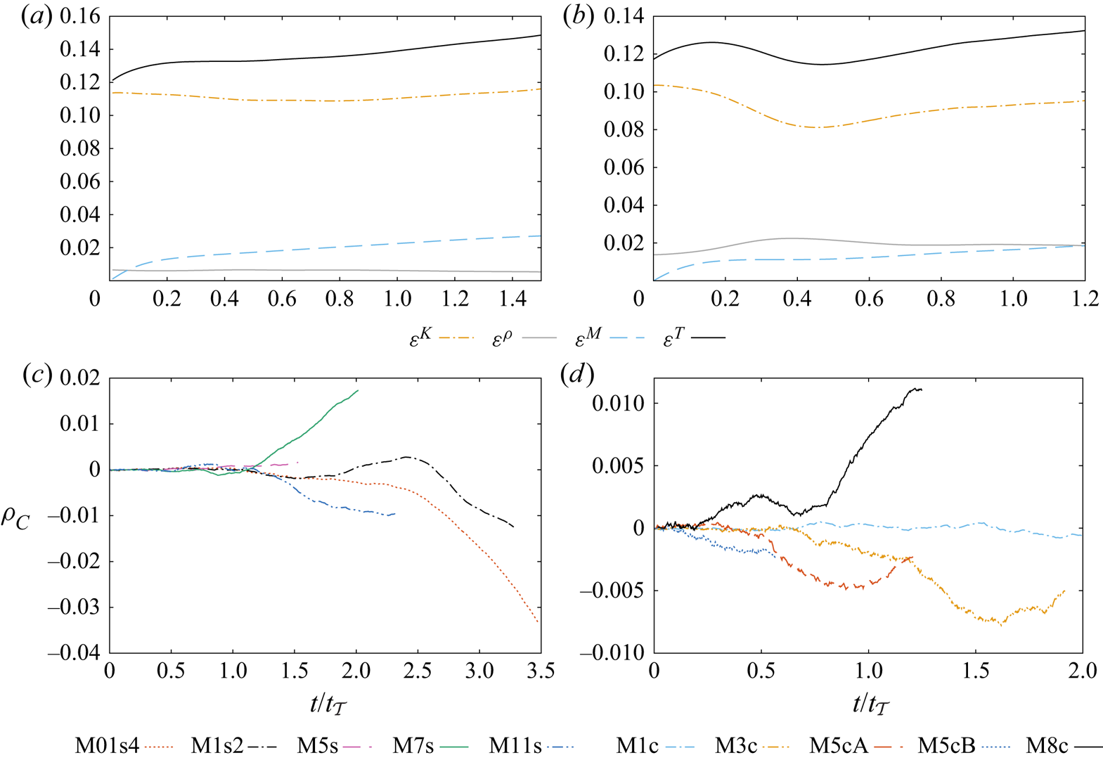
As magnetic energy is injected and transferred to larger scales, the total energy of the system tends to grow secularly (figure 3a,b). In compressible isothermal MHD, the total energy  ${\mathcal {E}}^{\textrm {T}}$ is the sum of the kinetic
 ${\mathcal {E}}^K=\frac {1}{2}\rho |{\boldsymbol {v}}^2|$, magnetic
 ${\mathcal {E}}^M=\frac {1}{2}|{\boldsymbol {b}}|^2$ and potential energy
 ${\mathcal {E}}^\rho =\rho c_s^2 \ln (\rho /\rho _0)$, stored as density fluctuations. Since no large-scale energy removal occurs, the asymptotic state of the system would be a condensate of magnetic helicity at the largest scales. This would strongly affect the locality of transfers and the spectral exponents (Alexakis et al. Reference Alexakis, Mininni and Pouquet2006; Linkmann & Dallas Reference Linkmann and Dallas2016). For this reason, in order to avoid the strong modification of the inverse transfer range by finite-size effects, the spectra are taken at an instant when an energetically dominant largest-scale magnetic structure has not yet emerged. The restricted spectral bandwidth of the numerical experiments thus requires caution with regard to the assumed stationarity of the established asymptotic scaling interval at
 $20 \leq K \leq 30$ or
 $15 \leq K \leq 25$. Any large-scale damping of magnetic energy or a magnetic large-scale condensate of finite energy would have a finite spectral width of influence reducing the observable scaling region from the large-scale side as does the finite spectral support of the magnetic driving from the small-scale side. The chosen set-up, although certainly not ideal, represents a pragmatic compromise between unquestionable statistical stationarity and a perfectly developed scaling region. Nevertheless, spectral scaling laws consistent with results from previous research in incompressible MHD and natural extensions of the same to compressible MHD have been found. Furthermore, the main results are confirmed through higher resolution runs (§ 5) and the main measurements of spectral exponents are presented as functions in time displaying acceptable saturation to constant levels (cf. figures in §§ 4.2–4.4).
(a,b) Time evolution of the kinetic, potential, magnetic and total energies for two representative M5s and M5cA runs. (c,d) Time evolution of the magnetic field–velocity alignment (normalised cross-helicity).

For all the runs, the magnetic field–velocity alignment,
 \begin{equation} \rho_{C}=\frac{\langle {\boldsymbol{v}} \cdot {\boldsymbol{b}} \rangle}{\sqrt{\langle |{\boldsymbol{v}}|^2 \rangle \langle |{\boldsymbol{b}}|^2 \rangle}}, \end{equation}
grows in time but remains very low (under 0.035, see figure 3c,d), so that the average alignment of magnetic and velocity field is small and the dynamics of the system are dominated by the direct cascades of kinetic and magnetic energies and the inverse transfer of magnetic helicity.
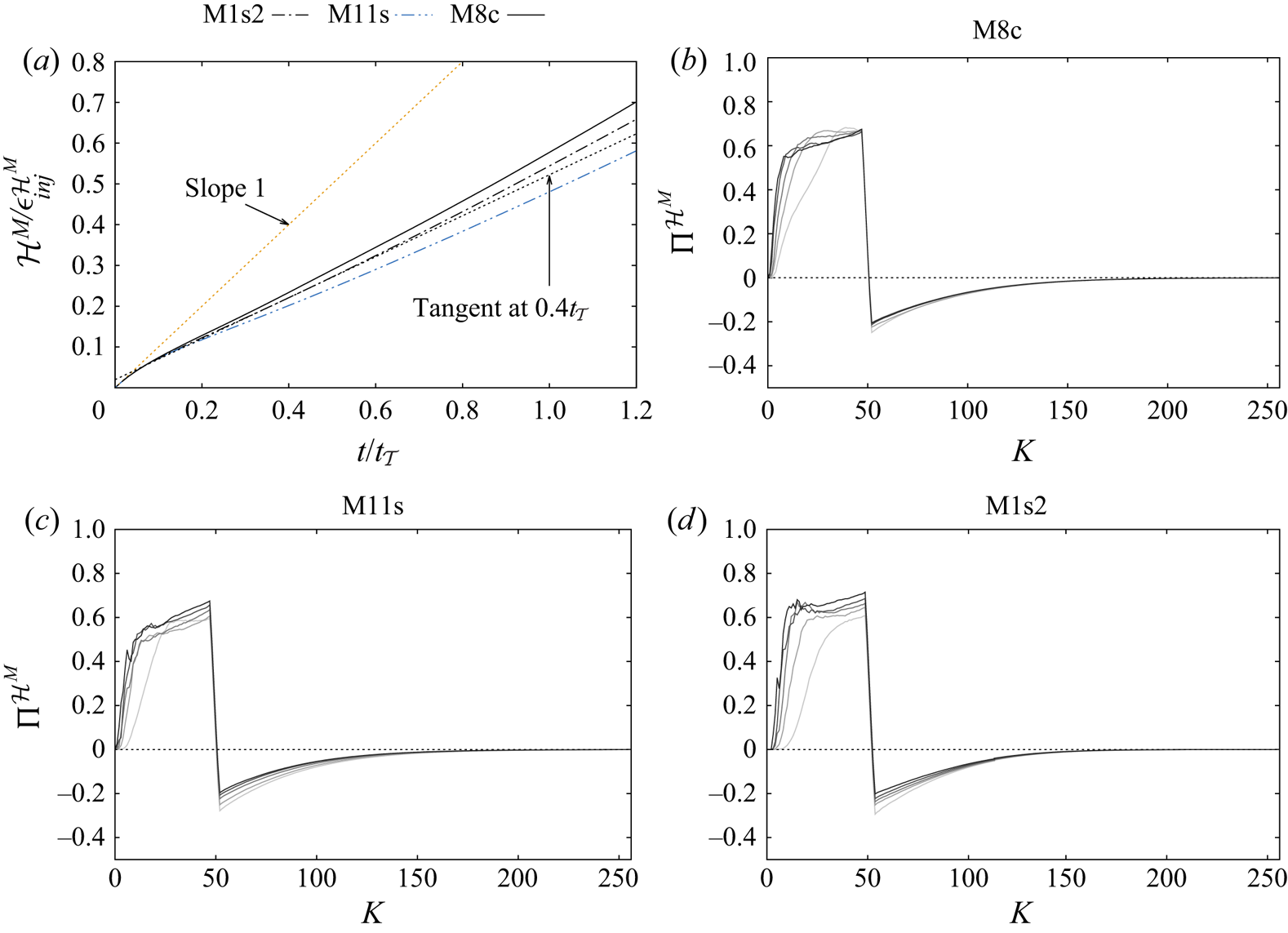
Figure 4(a) shows the total magnetic helicity in the system as a function of time for the M1s2, M11s and M8c runs, taken as representatives. The helicity is normalised by an estimate of its injection rate:  ${\epsilon ^{{{\mathcal {H}}^M}}_{inj}}=2{\epsilon ^{M}_{inj}}/(K_Ht_{\mathcal {T}})$ with
 $K_H=50$ the shell around which the electromotive forcing takes place. Therefore, if all the injected magnetic helicity were conserved, the normalised magnetic helicity in the system should be 1 at
 $t/t_{\mathcal {T}}=1$. Indeed, at early times, the total magnetic helicity follows this ideal evolution (indicated through the orange dotted line). However, due to numerical non-idealities, magnetic helicity is dissipated already at the forcing scale, and even partially transferred to smaller scales, where it is dissipated more rapidly, giving an effective rate of increase less than unity. The rate of increase is around 40 % to 60 % for these runs, since at
 $t/ t_{\mathcal {T}} = 1$ approximately half of the injected magnetic helicity is present in the system. These values are consistent with the ones obtained by considering the magnetic helicity flux
 ${\Pi }^{{{\mathcal {H}}^M}}(K)=\sum _{K_0=1}^K {\mathcal {T}}^{{{\mathcal {H}}^M}}(K_0)$ with
 ${\mathcal {T}}^{{{\mathcal {H}}^M}}=2{\mathcal {Q}}({\boldsymbol {b}},{\boldsymbol {v}}\times {\boldsymbol {b}})/{\epsilon ^{{{\mathcal {H}}^M}}_{inj}}$ the magnetic helicity transfer function normalised by its injection rate (figure 4b–d). For these curves, an approximate plateau is visible at larger scales, showing that approximately 50 % to 70 % of the injected magnetic helicity experience the inverse transfer, the rest being transferred to smaller scales or dissipated at the forcing scale. This plateau hints at a roughly constant flux of magnetic helicity to larger scales, even though a visible deviation exists that is probably due to non-local transport (Alexakis et al. Reference Alexakis, Mininni and Pouquet2006; Linkmann & Dallas Reference Linkmann and Dallas2016; Teissier Reference Teissier2020) and the finite size of the system. Not all the magnetic helicity transferred to larger scales is conserved, giving, hence, a lower rate of increase, since dissipation still occurs, especially when magnetic helicity has not yet reached the largest scales. This is why at later times the curves are not linear but convex, as can be seen through the tangent of the M1s2 curve, which lies under it. Indeed, as magnetic helicity is transferred to ever larger scales, dissipative effects are smaller so that magnetic helicity is better conserved.
(a) Evolution of the total magnetic helicity in the system, normalised by its estimated injection rate for some representative runs. The orange dotted line has a slope of 1, indicating the ideal evolution. The black dotted line is the tangent at the instant  $t=0.4t_{\mathcal {T}}$ of the M1s2 run, showing that these curves are convex at later times. (b–d) Magnetic helicity fluxes as a function of time for these three runs, five curves regularly spaced in the interval
 $]t_i,t_f]$ with
 $t_i$ the instant at which the electromotive driving is switched on and
 $t_f$ an instant at which
 ${\mathcal {I}}_{{{\mathcal {H}}^M}} \approx L/6$ – see relation (4.2). The darker the curve, the further forward time has advanced. The dotted line indicates zero on the ordinate.

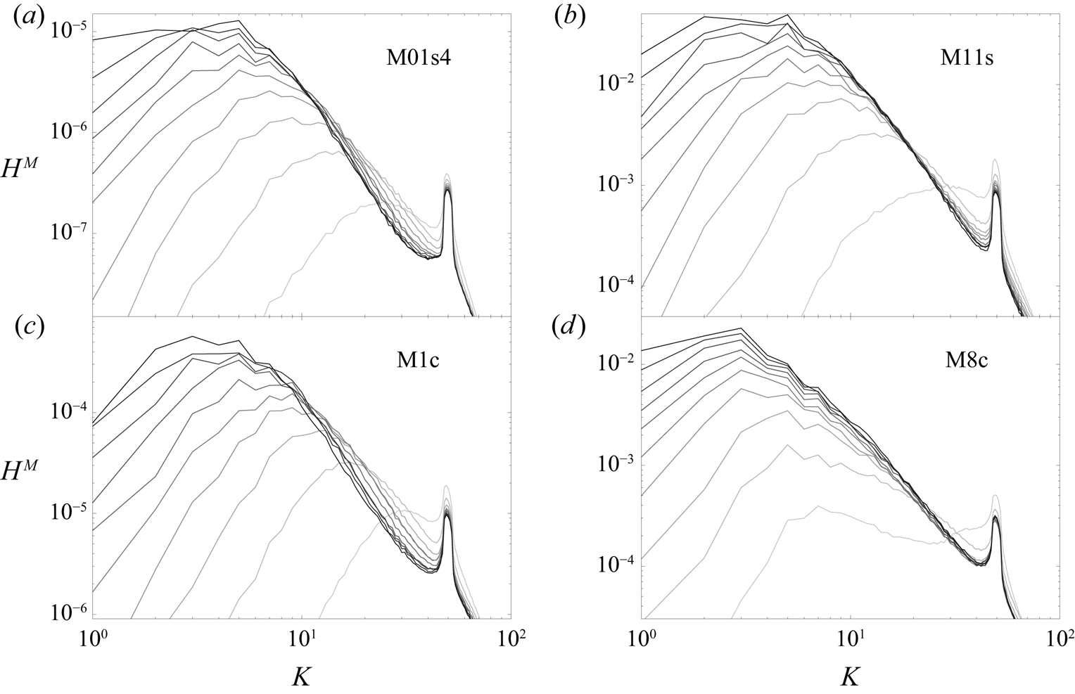
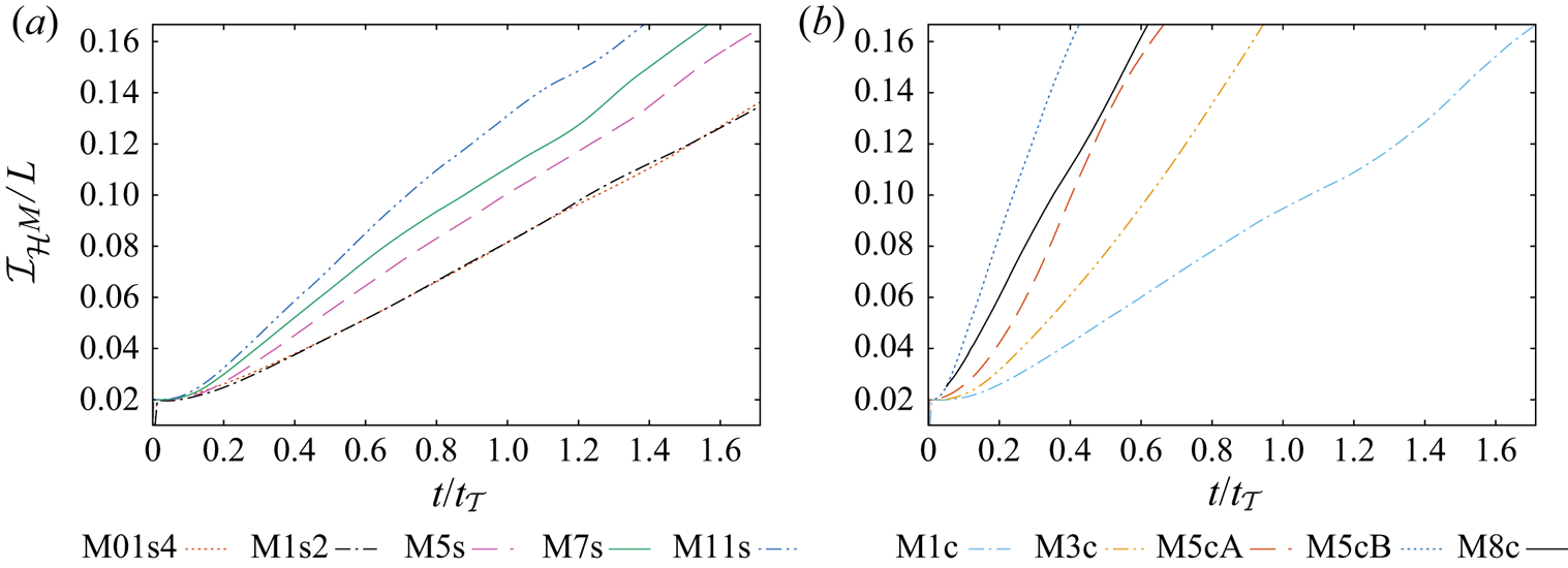
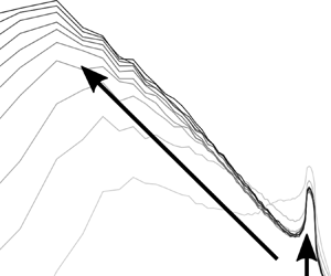
This inverse transfer of magnetic helicity in supersonic flows is illustrated in figure 5, where the time evolution of the magnetic helicity spectra  $H^M$ is shown for the least and most compressible cases considered. Figure 6 shows the time evolution of the magnetic helicity integral scale, defined as
 \begin{equation} {\mathcal{I}}_{{{\mathcal{H}}^M}}=L\frac{\displaystyle\int_{K} K^{{-}1} H^M_K \,{\rm d} K}{\displaystyle\int_{K} H^M_K \,{\rm d} K}. \end{equation}
Magnetic helicity is not a positive-definite quantity. Even though division by zero is in theory possible, since only magnetic helicity of one sign is injected, positive magnetic helicity dominates the system at all scales so that division by zero does not occur and considering this integral scale remains meaningful. The spectrum of the positive helical magnetic field  $H^M_+$ is approximately an order of magnitude larger than its negative part
 $H^M_-$ at all scales. The time is measured in units of the turbulent turnover time
 $t_{\mathcal {T}}=L/(2c_s{\mathcal {M}})$ of the hydrodynamic statistically stationary state of the flow, so that
 ${\mathcal {M}}$ designates the RMS Mach number before the injection of magnetic helicity. The inverse transfer occurs faster with increasing compressibility. While for the solenoidally driven runs, more than
 $1.5t_{\mathcal {T}}$ are required to reach the integral scale
 ${\mathcal {I}}_{{{\mathcal {H}}^M}}={L}/{6}$, less than approximately
 $0.6t_{\mathcal {T}}$ are needed for the compressively driven runs with
 ${\mathcal {M}} \gtrapprox 5$. For lower densities indeed, the Lorentz force has a greater impact on the velocity field's temporal evolution, since
 $\partial _t {\boldsymbol {v}} = \cdots + ({1}/{\rho }) (\boldsymbol {\nabla } \times {\boldsymbol {b}}) \times {\boldsymbol {b}}$, which backreacts on the magnetic field. At high compressibility, especially for compressively driven runs, large regions of low density are present (figure 1), which are associated with higher Alfvén velocities
 ${\boldsymbol {v_A}}={\boldsymbol {b}}/\sqrt {\rho }$ and hence faster dynamical time scales of magnetic field line reconfiguration
 $\propto l_{rec}/{\boldsymbol {v_A}}$, with
 $l_{rec}$ characterising the field-parallel extent of the magnetic reconnection region. Magnetic reconnection processes are required to achieve the topological changes of magnetic structures in the course of the inverse transport of magnetic helicity. Those changes are communicated along the affected field lines by Alfvén waves propagating at speed
 ${\boldsymbol {v_A}}$. This explains why for the M5cB run, whose initial condition presents a peak of the density p.d.f. at lower densities (figure 2d), the growth of the magnetic helicity integral scale is faster than for the M5cA run. This is also manifest in the time evolution of the magnetic helicity spectra: for the M8c run, in contrast to the M01s4, M11s and M1c runs, the magnetic helicity spectrum goes first to significantly larger scales before steepening its spectral slope (figure 5). This is also the reason of the choice of the turbulent turnover time of the mechanically forced velocity field as the unit of time in the plots. This quantity is constant by definition, contrary to the shorter magnetic inverse transfer time scale which evolves dynamically.
Time evolution of the magnetic helicity spectra for the least and most compressible runs. The darker the curve, the later it is. The 10 curves are equally spaced in time and correspond to the time intervals  $t\in [0.335t_{\mathcal {T}},3.35t_{\mathcal {T}}], [0.22t_{\mathcal {T}},2.2t_{\mathcal {T}}], [0.24t_{\mathcal {T}},2.4t_{\mathcal {T}}]$ and
 $[0.16t_{\mathcal {T}},1.6t_{\mathcal {T}}]$ for the M01s4, M11s, M1c and M8c runs, respectively.

Magnetic helicity integral scale time evolution.

4.2. Scaling relations: magnetic quantities
In order to compare the numerical models more easily with one another, the Fourier spectra of the different set-ups are considered at their respective instant in time when a magnetic helicity integral scale  ${\mathcal {I}}_{{{\mathcal {H}}^M}}\approx L /6$ is reached. This corresponds to
 $t/t_{\mathcal {T}}=2.13, 2.04, 1.73, 1.56, 1.38$ for the runs M01s4, M1s2, M5s, M7s, M11s, respectively, expressed in units of their respective large-eddy turbulent turnover time. For the compressively driven M1c, M3c, M5cA, M5cB, M8c runs, the respective instants are
 $t/t_{\mathcal {T}}=1.71, 0.95, 0.66, 0.42, 0.62$. This scale of
 $L/6$ is chosen in order to have a sufficiently large spectral distance between the magnetically forced and the largest scales, since a strong modification of the scaling range by the electromotive forcing at small scales and through large-scale condensation of magnetic helicity at the largest scales at late times due to the limited box size are expected. The magnetic-to-kinetic energy ratio
 ${\mathcal {P}}({\boldsymbol {b}})/{\mathcal {P}}(\sqrt {\rho }{\boldsymbol {v}})$ is of the order
 $10^{-2}$ at the largest scales
 $K<3$ due to the dominance of the kinetic forcing and the deliberate avoidance of a large-scale magnetic condensate. The spectral power-law exponent is determined by a logarithmic linear least squares fit (LSF) to the spectrum in a relevant domain, which depends on the run and the considered quantity. This domain is shown through vertical dashed lines in the figures.
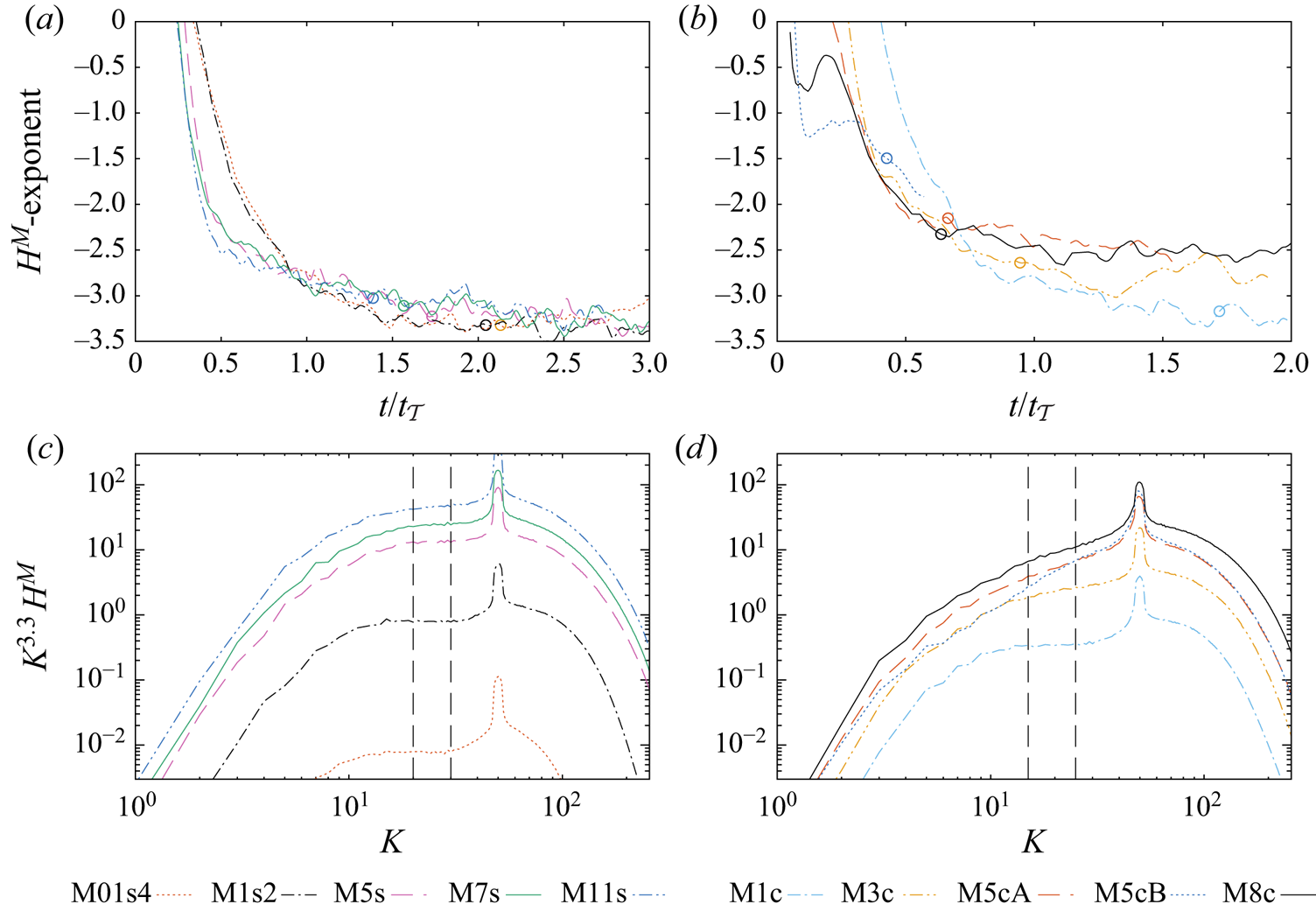
As expected from the presence of  $\boldsymbol {\nabla }\boldsymbol {\cdot } {\boldsymbol {v}}$ terms in the nonlinear evolution equations of magnetic helicity and magnetic energy (cf. (1.1)), the respective spectra display systematic changes when augmenting the Mach number of the flow. Those are more pronounced for compressively driven turbulence than for solenoidally driven flows. The low Mach number solenoidally driven M01s4 and M1s2 runs exhibit an approximate magnetic helicity power-law scaling
 $H^M \sim K^m$ with
 $m \approx -3.3$, gained from an LSF in the region
 $20 \leq K \leq 30$ (figure 7). This exponent is consistent with the observations in the incompressible case (Malapaka Reference Malapaka2009; Müller et al. Reference Müller, Malapaka and Busse2012). For higher RMS Mach numbers, increasing deviations are observed, namely
 $m\approx -3.2, -3.1$ and
 $-3.0$ for the M5s, M7s and M11s runs, respectively. Although significant, these deviations are clearly smaller than those obtained in the compressively forced runs. There, the spectra are clearly flatter at lower Mach numbers, see figure 7. For the M1c, M3c, M5cA and M8c runs, the exponents computed through an LSF in the region
 $15 \leq K \leq 25$ are
 $m \approx -3.2, -2.6, -2.2$ and
 $-2.3$, respectively. For supersonic compressively driven flows, the scaling exponent is very sensitive to the initial conditions: for example, the M5cB run, for which the magnetic helicity injection starts at a different instant during the same hydrodynamic statistically stationary state as the M5cA run, presents a significantly flatter spectrum with
 $m \approx -1.5$. This is linked with a peak of the initial condition's mass density p.d.f. at lower densities (figure 2d), so that faster time scales are expected for the M5cB run. This illustrates that the single realisations considered here could still be in a transient state. One would either need a significantly larger scale separation between the electromotive driving scale and the largest scales (which implies a very large resolution of the computational domain), or perform ensemble averaging over many realisations in order to obtain a less approximate dependency of the magnetic helicity exponent as a function of
 ${\mathcal {M}}$ when using a compressive forcing. These studies would imply significantly higher computational costs, which are beyond the resources available to the present investigation. Nevertheless, independent of possible transients, a clear tendency towards flatter exponents with increasing compressibility is observable, which can be largely compensated by an appropriate choice of variables, even with very different initial conditions, as shown below.
(a,b) Time evolution of the magnetic helicity power-law exponents. (c,d) Magnetic helicity spectra at an instant when  ${\mathcal {I}}_{{{\mathcal {H}}^M}}\approx {L}/{6}$ (shown through circles in panels (a,b)), compensated by
 $K^{3.3}$, since
 $H^M \sim K^{-3.3}$ in the incompressible case. The exponents measured in panels (a,b) are gained through an LSF in the region delimited with vertical dashed lines in panels (c,d) (here
 $20 \leq K \leq 30$ and
 $15 \leq K \leq 25$ for the solenoidally driven and compressively driven runs, respectively).

The spectra of the positive helical magnetic field  $H^M_+$ are close to those of the total magnetic helicity
 $H^M=H^M_+-H^M_-$, which is expected since
 $H^M_+$ is approximately an order of magnitude greater than
 $H^M_-$ at all scales. After a time of the order of
 $t_{\mathcal {T}}$, the exponents measured are close to
 $-3.2, -3.2, -3.1, -3.0$ and
 $-2.9$ for the M01s4, M1s2, M5s, M7s and M11s runs, respectively, and close to
 $-3.0, -2.6, -2.1, -1.5$ and
 $-2.3$ for the M1c, M3c, M5cA, M5cB and M8c runs, respectively. The negative helical magnetic field
 $H^M_-$ scales as
 $-2.7, -2.5, -2.1, -2.2, -2.0$ (M01s4, M1s2, M5s, M7s, M11s runs) and
 $-2.4, -2.0, -1.7, -1.1, -1.7$ (M1c, M3c, M5cA, M5cB, M8c runs).
The same tendency is observed for the magnetic energy spectra: the scaling exponents are close to the  $-2.1$ observed in the incompressible case (Malapaka Reference Malapaka2009; Müller et al. Reference Müller, Malapaka and Busse2012) for the low Mach number M01s4, M1s2 and M1c runs, flatter with increasing compressibility for the solenoidally driven runs and significantly flatter for the compressively driven runs already at lower initial RMS Mach numbers (curves not shown here).
In the incompressible case, the Alfvén velocity  ${\boldsymbol {v_A}}={\boldsymbol {b}}/\sqrt {\rho }$ (with
 $\rho$ a constant) and the magnetic field are in essence the same quantity. However, in the compressible case, low density regions are associated with higher Alfvén velocities, so that the dynamical time scales are shorter there. For this reason, it is tempting to consider the power spectrum of the Alfvén velocity
 $E^A={\mathcal {P}}({\boldsymbol {v_A}})$ as well as the cospectrum of the Alfvén velocity and its curl
 $H^A={\mathcal {Q}}({\boldsymbol {v_A}},\boldsymbol {\nabla } \times {\boldsymbol {v_A}})$, which is the helicity of the Alfvén velocity, a quantity hereafter called ‘Alfvénic helicity’. In the incompressible case, the Alfvénic helicity is
 ${\boldsymbol {b}} \cdot {\boldsymbol {j}}/\rho$ and corresponds thus to the current helicity
 $H^J = (({2{\rm \pi} }/{L})K)^2 H^M$, which exhibits an approximate scaling law
 $H^J \sim K^{-1.3}$ (Malapaka Reference Malapaka2009; Müller et al. Reference Müller, Malapaka and Busse2012).
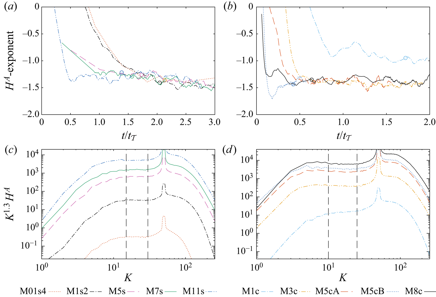
The Alfvénic helicity and Alfvén velocity power spectra display only a weak dependence on the compressible character of the forcing and the flow. While the magnetic energy and helicity spectra become flatter with increasing compressibility, for the Alfvénic helicity the incompressible scaling exponent  $-1.3$ is approximately observed for all simulations with
 ${\mathcal {M}} \gtrsim 3$ as well (see figure 8). This is in particular the case for the M5cA and M5cB runs, which present very different
 $H^M$ scaling exponents. The scaling exponents of
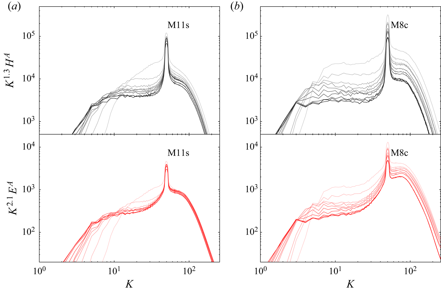
 $E^A$, which approach asymptotically
 $-1.8$ for the most compressible runs (see figure 9), are also closer to the
 $-2.1$ scaling for the magnetic energy in the incompressible case (Malapaka Reference Malapaka2009; Müller et al. Reference Müller, Malapaka and Busse2012) and present a weaker dependence on the flow's compressibility as compared with
 $E^M$.
Same as figure 7, but for the Alfvénic helicity  $H^A$ which exhibits a
 $K^{-1.3}$ scaling in the incompressible case.

Time evolution of  $H^A$ and
 $E^A$ for the M11s and M8c runs, compensated by
 $K^m$ with
 $-m$ the scaling exponent in the incompressible case. The spectra are snapshots taken at different instants (the darker, the later), from
 $t=t_f/10$ to
 $t_f=2.2t_{\mathcal {T}}$ and
 $t_f=1.6t_{\mathcal {T}}$ for the M11s and M8c runs, respectively.

This universality of the exponents over a wide range of compressibility suggests a systematic scale-dependent correlation between the density and the magnetic fields, which is the object of further investigations. The M1c run may present different dynamics since its velocity compressive ratio  ${\mathcal {P}}^{comp}({\boldsymbol {v}})/{\mathcal {P}}({\boldsymbol {v}})$ remains large in the inverse transfer region (see figure 10). This is reflected by the lack of low density regions in this simulation.
(a,b) Time-averaged velocity compressive ratio during the hydrodynamic statistically stationary state, exhibiting values close to 1/3 for the solenoidally driven supersonic runs and 1/2 for the supersonic compressively driven ones in a reasonable wavenumber range, consistently with Federrath et al. (Reference Federrath, Roman-Duval, Klessen, Schmidt and Mac Low2010). (c,d) Snapshots of the compressive ratio at an instant when  ${\mathcal {I}}_{{{\mathcal {H}}^M}}\approx L /6$: all supersonic runs exhibit a compressive ratio close to 0.2, independently of the mechanical forcing type. The M1c run continues to exhibit a large compressive ratio.

4.3. Scaling relations: kinetic quantities
In the incompressible case, the kinetic energy and helicity exhibit approximate scaling laws with exponents close to  $-1.2$ and
 $-0.4$, respectively (Malapaka Reference Malapaka2009; Müller et al. Reference Müller, Malapaka and Busse2012). In the compressible case, several alternative definitions for the incompressible kinetic energy have been considered in the literature, e.g.
 $E^V={\mathcal {P}}({\boldsymbol {v}})$, i.e. the specific kinetic energy spectrum,
 $E^K={\mathcal {P}}(\boldsymbol {w})$, with
 $\boldsymbol {w}=\sqrt {\rho }{\boldsymbol {v}}$, which is dimensionally a kinetic energy spectrum,
 $E^U={\mathcal {P}}(\boldsymbol {u})$, with
 $\boldsymbol {u}=\rho ^{1/3}{\boldsymbol {v}}$, a quantity for which the Kolmogorov spectrum with exponent
 $-\frac {5}{3}$ is recovered in compressible hydrodynamic turbulence with a low
 $\boldsymbol {\nabla }\boldsymbol {\cdot }{\boldsymbol {v}}$ component (Fleck Reference Fleck1996; Kritsuk et al. Reference Kritsuk, Norman, Padoan and Wagner2007; Federrath et al. Reference Federrath, Roman-Duval, Klessen, Schmidt and Mac Low2010; Federrath Reference Federrath2013),
 $\frac {1}{2}{\mathcal {Q}}(\rho {\boldsymbol {v}},{\boldsymbol {v}})$, the cospectrum of velocity and momentum (or more generally, any cospectrum
 $\frac {1}{2}{\mathcal {Q}}(\rho ^{\alpha }{\boldsymbol {v}},\rho ^{1-\alpha }{\boldsymbol {v}})$ with
 $\alpha \in [0,1]$ Aluie (Reference Aluie2013)), or
 $E^{V,sol}={\mathcal {P}}^{sol}({\boldsymbol {v}})$, the solenoidal part of the specific kinetic energy spectrum.
From the above-mentioned quantities, the specific kinetic energy spectrum  $E^V={\mathcal {P}}({\boldsymbol {v}})$ and its solenoidal part
 $E^{V,sol}$ (shown in figure 11) present the most universal behaviour, with an exponent close to
 $-1.2$ for all the runs. The deviations from the
 $-1.2$ exponent become weaker at later times for the M01s4 and M1s2 runs and the stronger deviations for the M1c run are due to the high velocity-spectrum compressive ratio. The other above-mentioned spectra, as well as that of the density, are displayed in appendix A.
Same as figure 7, but for the solenoidal part of the specific kinetic energy spectrum  $E^{V,sol}$ which exhibits a
 $K^{-1.2}$ scaling in the incompressible case.

As for the kinetic helicity, the  $-0.4$ incompressible exponent appears to be the asymptotic behaviour for all levels of higher compressibility (figure 12). The negative kinetic helicity values at large scales for some runs are not an established feature of the inverse transfer experiment: their sporadic occurrence is a consequence of the random mechanical forcing. The spectral transient region influenced by the small-scale magnetic driving is wider at lower Mach numbers. This is probably linked with the presence of a large-scale mechanical driving in the present experiments, as compared with those of Müller et al. (Reference Müller, Malapaka and Busse2012). In hydrodynamic turbulence, the energy cascade tends to an equipartition of energy in the positive and negative helical parts of the velocity field at small scales, so that the kinetic helicity tends to zero (Chen, Chen & Eyink Reference Chen, Chen and Eyink2003). On the other hand, the injection of magnetic helicity at small scales leads to the generation of kinetic helicity. It is plausible that for runs with pronounced compressible effects and low density regions, the dynamical time scale of the kinetic helicity production is faster than that of the direct energy cascade leading to vanishing kinetic helicity, so that the
 $-0.4$ exponent observed in the absence of large-scale mechanical driving is recovered, but only for the supersonic flows. As shown in figure 12(c), a low-Mach-number run performed in the absence of a large-scale mechanical driving gives a kinetic helicity scaling compatible with
 $-0.4$.
(a,b) Kinetic helicity spectra  $H^V$ at an instant when
 ${\mathcal {I}}_{{{\mathcal {H}}^M}}={L}/{6}$ compensated by
 $K^{0.4}$. (c) time evolution of
 $H^V$, compensated by
 $K^{0.4}$, for a low-Mach-number run without large-scale mechanical driving, with
 ${\epsilon ^{M}_{inj}}=7\times 10^{-4}$ (for which
 ${\mathcal {M}} \approx 0.2$). The curves are equally spaced in time from an instant when
 ${\mathcal {I}}_{{{\mathcal {H}}^M}}\approx L /19$ until
 ${\mathcal {I}}_{{{\mathcal {H}}^M}} \approx L/3$. The darker the curve, the larger
 ${\mathcal {I}}_{{{\mathcal {H}}^M}}$.

4.4. Alfvénic balance
The observations presented so far suggest that the Alfvénic balance found in the incompressible case (relation (3.1)) can be extended to the compressible case when considering, instead of the current helicity  $H^J$ and the magnetic energy
 $E^M$, the Alfvénic helicity
 $H^A$ and the power spectrum of the Alfvén velocity
 $E^A$, respectively, and by considering the specific kinetic energy
 $E^V$ or its solenoidal part. Since the energy associated with
 $H^A$ and the kinetic helicity
 $H^V$ is the solenoidal part of
 $E^A$ and of
 $E^V$, respectively, the following extension of the Alfvénic balance in the compressible case is proposed:
 \begin{equation} \left(\frac{E^{V,sol}}{E^{A,sol}}\right)^{\gamma} \propto \frac{H^V}{H^A}. \end{equation}
This choice is a straightforward extension of the balance in the incompressible case, where only solenoidal modes exist. It suggests that the shear, not the compressive waves, balance the twisting in compressible turbulence as well (cf. text around relation (3.1)). To test this relation, the ratio
 \begin{equation} \varLambda(r_H,r_E,\gamma)=\frac{r_E^\gamma}{r_H}, \end{equation}
with  $r_H=r_{H^V_A}=H^V/H^A$ and
 $r_E=r_{E^{V,sol}_{A,sol}}=E^{V,sol}/E^{A,sol}$ is plotted in figure 13 for the different runs and different
 $\gamma$. This relation is well followed for the least compressible M01s4, M1s2 and M1c runs with
 $\gamma =2$, with
 $\varLambda \approx 1.1 \pm 0.3$ on the domain
 $20 \leq K \leq 44$, consistent with Müller et al. (Reference Müller, Malapaka and Busse2012). For the most compressible cases, the curves for the M3c, M5cA M5cB and M8c runs show a similar behaviour for
 $\gamma =1$, with
 $\varLambda \approx 2.7 \pm 0.5$ on the
 $13 \leq K \leq 33$ domain. Regarding the supersonic solenoidally driven runs, they present an intermediate behaviour: for
 $\gamma =2$, the M5s curve would be included in the ‘M01s4–M1s2–M1c bundle’ on the domain
 $12 \leq K \leq 40$, whereas for
 $\gamma =1$, the M11s curve would be included in the ‘M3c–M5c–M8c bundle’ on the domain
 $16 \leq K \leq 31$.
Test of the Alfvénic balance (relation (4.3)) by plotting  $\varLambda (r_H,r_E,\gamma )=r_E^\gamma /r_H$ (relation (4.4)) with
 $r_H=r_{H^V_A}=H^V/H^A$ and
 $r_E=r_{E^{V,sol}_{A,sol}}=E^{V,sol}/E^{A,sol}$ for different runs and different exponents
 $\gamma$: (a) for the subsonic and transonic runs,
 $\gamma =2$, compatible with the results in the incompressible case; (b) for the supersonic compressively driven runs, which verify the Alfvénic balance for
 $\gamma =1$; (c,d) for the supersonic solenoidally driven runs, which present an intermediate behaviour with respect to the
 $\gamma$ exponent.

Replacing the solenoidal parts  $E^{V,sol}$ and
 $E^{A,sol}$ by the total energies
 $E^V$ and
 $E^A$ in
 $\varLambda$ also gives a good horizontal for the high Mach number compressively driven runs. The ‘M3c–M5c–M8c bundle’ verifies then
 $\varLambda \approx 3 \pm 0.5$ on the same
 $13 \leq K \leq 33$ domain. With this choice, however, the M1c curve does not stay in the ‘M01s4–M1s2’ bundle, which is why the choice of relation (4.3) is preferred.
Although other variants of relation (4.3) are partially consistent with the data as well, this choice shows overall the best agreement with the simulations, as well as the least spread between the curves. This also holds at higher numerical resolution, which is not the case for some other possibilities, as shown in § 5.
5. Confirmation at higher resolution
In addition to the already mentioned inaccuracies of the present numerical experiments (see § 2.3), in the framework of the fallback approach, not all cells are reconstructed at higher order. For the most compressible M11s and M8c runs, a little more than 50 % of the reconstructions occur indeed at third order or lower. It is hence important to check that the results presented here are reasonably well converged, both with respect to the resolution and the numerical scheme's order. Therefore, some additional runs are considered: the M1s2LR and M1s2HR runs, which are lower resolution ( $256^3$) and higher resolution (
 $1024^3$) runs, respectively, and the M1s2LO run which is done at resolution
 $512^3$ but using a second-order scheme. Similarly, additional runs for the M8c case are considered, labelled analogously ‘M8cLR’, ‘M8cHR’ and ‘M8cLO’. For this supersonic compressively driven run, the time step
 $\Delta t$ becomes very small at higher resolutions, due to very high Alfvén speeds in low density regions, so that only an early instant in time is considered, when
 ${\mathcal {I}}_{{{\mathcal {H}}^M}} \approx 0.045 L$, but where scaling behaviour is already observed.
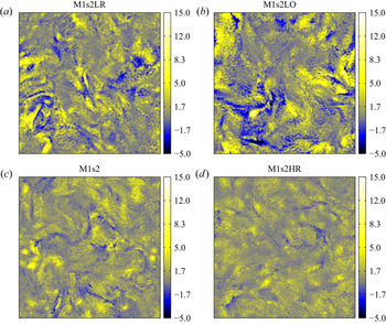
Finer structures are visible for the M1s2 family in the magnetic helicity density slices with increasing resolution and/or using a higher-order scheme (figure 14), as a result of accuracy gain and significant reduction of numerical dissipation. The level of detail of the  $512^3$ lower-order run is very similar to the one of the
 $256^3$ higher-order run, showing the benefits of using higher-order numerics: even though they are computationally more expensive at a given resolution, they allow a comparable accuracy at lower resolution, resulting in a net performance gain.
Magnetic helicity density slices, normalised by the mean magnetic helicity in the system, at an instant when  ${\mathcal {I}}_{{{\mathcal {H}}^M}}\approx \frac {1}{6}L$.

For the M1s2 family, a scaling exponent consistent with  $H^M \sim K^{-3.3}$ is observed as well for the higher resolution run (figure 15a). The lower resolution and lower-order runs also seem to converge to this exponent, but more slowly (figure 15b). The Alfvénic balance (relation (4.3)) is also well verified with
 $\gamma =2$ (figure 15c). Similarly, for the M8c family, the scaling exponents for the Alfvénic helicity are consistent with
 $H^A \sim K^{-1.3}$ for all the runs and the Alfvénic balance (4.3) looks well converged for
 $\gamma =1$ (figure 15d,e). For these supersonic runs, the lower-order run M8cLO seems to deviate less than the lower resolution M8cLR one as compared with the M8cHR run, in contrast with the M1s2LR and M1s2LO runs, which both give significant deviations from the
 $512^3$ and
 $1024^3$ fourth-order runs. This means that the effect of lowering the order has less impact on numerical dissipation, than changing the spatial resolution in case of shock fronts which should actually dominate dissipation for M8c. Hence, at second order, the reconstruction is already at its limit in resolving the shock fronts at the given resolution. Thus the results regarding shocks and dissipation cannot be improved by raising the order. This does not, however, mean that we do not get significant improvements in smooth regions.
Confirmation of results through a resolution/numerical-order study. The LR and HR labels stand for lower ( $256^3$) and higher (
 $1024^3$) resolution, respectively, and the LO for lower-order (second-order) numerics. Panels (a–c), above the dashed line, are for the M1s2 family; panels (d–h), under the line, are for the M8c family. (a) Compensated magnetic helicity spectra for the M1s2 family, the dashed vertical lines delimiting
 $20 \leq K \leq 30$ show the domain where the LSF occurs in panel (b), which shows the time evolution of the magnetic helicity scaling exponent. (c) Verification of the Alfvénic balance. (d) Compensated Alfvénic helicity spectra for the M8c family. (e–h) Different Alfvénic balance variants (where
 $\varLambda (r_H,r_E,\gamma )=r_E^\gamma /r_H$, see relation (4.4)) for the M8c family, with
 $r_{H^V_J}=H^V/H^J$ and similarly
 $r_{E^{K}_{A}}=E^K/E^A, r_{E^{K}_{M}}=E^K/E^M$.

Other variants of the Alfvénic balance, shown in figure 15(f–h) with different choices for  $(r_H,r_E,\gamma )$ in relation (4.4), which also present a horizontal line at resolution
 $512^3$, present deviations from the horizontal at the higher
 $1024^3$ resolution as well as a greater resolution dependence. This hints at a better validity of the variant expressed in relation (4.3).
These observations suggest that even though studies at higher resolutions would be beneficial in capturing all the turbulent fine structures, the observed scaling laws are quite robust.
6. Conclusion
Similarly to the incompressible case, spectral scaling laws are observed for the magnetic helicity inverse transfer in supersonic compressible isothermal MHD turbulence. This has been shown through direct numerical simulations, starting with mechanically driven statistically stationary states of hydrodynamic turbulence, with RMS Mach numbers ranging from approximately 0.1 to 11 for a purely solenoidal forcing and from approximately 1 to 8 for a purely compressive driving, to which small-scale magnetic helical fluctuations are injected. The higher-order numerics allow results of convincing accuracy already at resolution  $512^3$: in spite of well known numerical inaccuracies (numerical dissipation, energy excess towards the grid-scale or ‘bottleneck effect’), the main results seem well converged when comparing with
 $256^3$ and
 $1024^3$ runs. Of course, more investigations are needed to solidify the findings of this study.
The scaling exponents obtained are generally in good agreement with those found in the incompressible case for subsonic and transonic solenoidally driven flows. In particular, the magnetic helicity spectrum scales as  $K^{m}$ with
 $m \approx -3.3$. The spectra become increasingly flatter with higher compressibility. The deviations are, however, relatively small for the solenoidally driven runs even at RMS Mach numbers of the order of 10 as compared with the purely compressive driving, where the spectra are significantly flatter already at a RMS Mach number around 3 in the initial hydrodynamic statistically stationary state. Due to the relatively limited scale separation between the electromotive driving and the largest scales, these results should be considered with appropriate caution, since transient behaviours as well as finite-resolution effects could still play a role.
In the interstellar medium, both cases of a purely solenoidal or a purely compressive forcing are very unlikely to happen (Federrath et al. Reference Federrath, Roman-Duval, Klessen, Schmidt and Mac Low2010). The present results suggest that effects of compressibility have a significant impact on the magnetic helicity dynamics in astrophysical systems of interest already at relatively low RMS Mach numbers, especially in situations where the turbulence drivers are rather compressive.
An appropriate change of variable, namely considering the Alfvén velocity  ${\boldsymbol {v_A}}={\boldsymbol {b}}/\sqrt {\rho }$ instead of the magnetic field, alleviates the differences between the compressible and the subsonic/transonic solenoidally driven runs. The cospectrum of the Alfvén velocity and its curl, named here ‘Alfvénic helicity’, presents for all the runs but the M1c one similar scaling, consistent with the incompressible case one, scaling as
 $K^{m}$ with
 $m \approx -1.3$. Even though this result is observed over a small range in spectral space, it suggests a universality in the inverse transfer dynamics, valid over a wide range of compressibility.
Lastly, the ‘Alfvénic balance’ (a quasi-equipartition in terms of magnetic and kinetic energies and helicities) observed in incompressible MHD has been extended using an appropriate change of variables. Further investigations of the balance relation are under way.
In the present numerical experiments, magnetic helicity of one sign dominates the system at all scales. In astrophysical systems of interest, however, magnetic helical components of mixed signs are expected to be present. In this context, the scaling laws may differ. Nevertheless, the preliminary study presented here in the simpler case of one helical sign injection, provides insights which should help the interpretation of future results in more general cases.
Acknowledgements
The authors acknowledge the North-German Supercomputing Alliance (HLRN) for providing HPC resources that have contributed to the research results reported in this paper. Computing resources from the Max Planck Computing and Data Facility (MPCDF) are also acknowledged.
Funding
J.M.T. gratefully acknowledges support by the Berlin International Graduate School in Model and Simulation based Research (BIMoS).
Declaration of interests
The authors report no conflict of interest.
Appendix. Spectra linked with kinetic energy
As mentioned in § 4.3, the (specific) kinetic energy spectrum in the incompressible case where the mass density  $\rho$ is constant, can correspond to several quantities in the compressible case. Figure 16 shows some possibilities not displayed in the main text, at an instant when
 ${\mathcal {I}}_{{{\mathcal {H}}^M}} \approx L/6$. The spectra are compensated by
 $K^{1.2}$ since the scaling observed in the incompressible case is
 $E^V={\mathcal {P}}({\boldsymbol {v}}) \sim K^{m}$ with
 $m\approx -1.2$ (Müller et al. Reference Müller, Malapaka and Busse2012). This
 $E^V$ scaling is well verified in the supersonic flows studied here also. Deviations are observed when considering
 ${\mathcal {P}}(\rho ^{1/3}{\boldsymbol {v}})$,
 ${\mathcal {P}}(\rho ^{1/2}{\boldsymbol {v}})$ or the cospectrum
 $\frac {1}{2}{\mathcal {Q}}(\rho {\boldsymbol {v}},{\boldsymbol {v}})$.
Different variants corresponding to the (specific) kinetic energy in the incompressible case (where  ${\mathcal {P}}({\boldsymbol {v}}) \sim K^{-1.2}$), taken at an instant when
 ${\mathcal {I}}_{{{\mathcal {H}}^M}} \approx L/6$.

Spectral data of the mass density field are displayed in figure 17. The time evolution of the exponents displays large variations on time scales smaller than  $t_{\mathcal {T}}$, especially for the supersonic compressively driven runs, which are very probably associated with sound waves and shocks. The spectral exponents are generally between
 $-1$ and
 $-0.5$ for solenoidally driven flows and steeper (between
 $-1.7$ and
 $-1$) for compressively driven ones. As the Mach number is decreased, the spectral interval directly influenced by the small-scale forcing appears to become wider, reducing the observable scaling region.
Power spectrum of the density at the same instant for which  ${\mathcal {I}}_{{{\mathcal {H}}^M}} \approx L/6$ (c,d), and time evolution of its scaling exponent in the region delimited by vertical black dashed lines,
 $15\leq K \leq 25$ (a,b). The subsonic run M01s4 for which the density is everywhere close to the mean density
 $\rho _0=1$ is not shown.