





1. Stochastic heat equation
We consider the following stochastic heat equation (SHE) with a multiplicative noise, posed on the circle  $\mathbb{T} = \mathbb{R}/(2\pi \mathbb{Z})$:
 \begin{equation}
\begin{cases}
\partial_t u +(1- \partial_x^2) u = u \phi \zeta\\
u|_{t = 0} = u_0.
\end{cases}
\end{equation}
Here,  $\phi$ is a Hilbert–Schmidt operator from
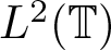 $L^2(\mathbb{T})$ to
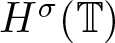 $H^\sigma(\mathbb{T})$ for some
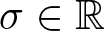 $\sigma \in \mathbb{R}$ (such that the noise
 $\phi \zeta$ has spatial regularity
 $\sigma$; more precisely,
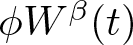 $\phi W^\beta(t)$ has spatial regularity
 $\sigma$, where
 $W^\beta$ is as in (1.5)) and
 $\zeta$ denotes a fractional-in-time/white-in-time and white-in-space noise. Heuristically, one may think of
 $\zeta$ as
 \begin{equation}
\text{‘}\,\zeta = \langle \partial_t \rangle^{-\alpha}\xi\,\text{’}
\end{equation}
for some 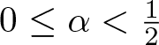 $0 \le \alpha \lt \frac 12$, where
 $\langle \,\cdot\, \rangle = (1+ |\cdot|^2)^\frac12$ and
 $\xi$ denotes a (Gaussian) space-time white noise on
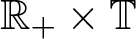 $\mathbb{R}_+ \times \mathbb{T}$ whose space-time covariance is (formally) given by
 \begin{align*}
\mathbb{E}[ \xi(t_1, x_1)\xi(t_2, x_2) ] = \delta(t_1 - t_2) \delta (x_1 - x_2)
\end{align*}
for 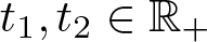 $t_1, t_2 \in \mathbb{R}_+$ and
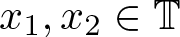 $x_1, x_2 \in \mathbb{T}$ with
 $\delta$ denoting the Dirac delta function. See (1.7) for the precise meaning of
 $\zeta$.
We say that  $u$ is a solution to (1.1) with initial data
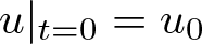 $u|_{t = 0} = u_0$ if
 $u$ satisfies the following Duhamel formulation (= mild formulation):
 \begin{equation}
u(t) = S(t) u_0 + \Psi(u)(t),
\end{equation}
where 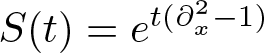 $S(t) = e^{t(\partial_x^2 - 1)}$ denotes the heat semigroup and
 $\Psi(u)$ denotes the stochastic convolution, representing the effect of the multiplicative noise, given by
 \begin{equation}
\Psi(u)(t) =
\int_0^t S(t-t')\big[ u(t') \phi dW^\beta (t')\big].
\end{equation}
Here,  $W^\beta$ denotes the cylindrical fractional Wiener process on
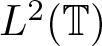 $L^2(\mathbb{T})$ given by
 \begin{equation}
W^\beta(t)
= \sum_{n\in \mathbb{Z}}
B_n(t) e_n,
\end{equation}
where  $e_n(x) = e^{in x}$ and
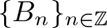 $\{B_n \}_{n \in \mathbb{Z}}$ is a family of independent complex-valued fractional Brownian motions with Hurst parameter
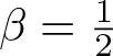
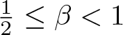 $\frac 12 \le \beta \lt 1$ (note that
 $\alpha$ in (1.2) is given by
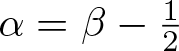 $\alpha = \beta -\frac 12$), conditioned that
 \begin{equation}
B_{-n} = \overline{B_n}, \quad n \in \mathbb{Z}.
\end{equation}
Namely, we have
 \begin{equation}
\zeta = \partial_t W^\beta.
\end{equation}
When 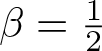 $\beta = \frac 12$, the sequence
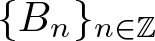 $\{B_n \}_{n \in \mathbb{Z}}$ reduces to a family of independent standard complex-valued Brownian motions, satisfying (1.6), and thus
 $W^{\frac 12}$ corresponds to an
 $L^2$-cylindrical Wiener process. See §3.1 for a review on fractional Brownian motions and stochastic integrals with respect to them.
Our main goal in this paper is to revisit pathwise well-posedness issues for SHE (1.1), previously studied in [Reference Gerasimovičs and Hairer14, Reference Gubinelli, Lejay and Tindel18, Reference Gubinelli and Tindel19, Reference Hairer and Pardoux21]. In [Reference Gubinelli and Tindel19], Gubinelli and Tindel generalized Lyons’ rough path theory [Reference Lyons23] and developed an algebraic integration theory adapted to an analytic semigroup. More precisely, they extended the sewing lemma and controlled paths, introduced in a seminal work [Reference Gubinelli15] by Gubinelli, to the current convolution setting. (There are various names attached to the approach in [Reference Gubinelli and Tindel19]. See, for example, [Reference Friz and Hairer13, Exercise 4.16]. Following [Reference Gubinelli and Tindel19], we use the term ‘convolution’ since relevant operators (such as  $\mathbf{X}^1$ in (1.11)) have a convolution-in-time structure.) In particular, by constructing the stochastic convolution
 $\Psi(u)$ in (1.4) as a convolution Young/rough integral, they proved the well-posedness of SHE (1.1) with
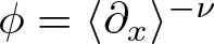 $\phi = \langle \partial_x \rangle^{-\nu}$. See §4.1 and §5.1 below for a review on the algebraic part of their approach.
In this paper, we will employ the algebraic structure introduced in [Reference Gubinelli and Tindel19] but introduce an improvement on the analytical side by incorporating the random tensor estimate, originally introduced in the context of random variables by Deng, Nahmod, and Yue [Reference Deng, Nahmod and Yue12], to the current stochastic setting. In a series of recent works [Reference Chapouto, Gubinelli, Li, Li and Oh4–Reference Chapouto, Li, Oh and Zheng7, Reference Oh and Shao27], the last two authors with A. Chapouto developed pathwise well-posedness theory of stochastic dispersive PDEs with multiplicative noises, which had been open for more than several decades since the inception of Ito solution theory (and random field solution theory) in [Reference Walsh33] for wave equations and in [Reference de Bouard and Debussche10, Reference de Bouard and Debussche11] for Schrödinger equations. A key ingredient in this development was the random tensor estimate for multiple stochastic integrals (for both the fractional-in-time and white-in-time cases); see Lemma 3.5. See §3 for a further discussion on the random tensor estimate for multiple stochastic integrals. The random tensor estimate allows us to estimate operator norms of relevant (random) drivers in a much more effective manner as compared to [Reference Gubinelli and Tindel19], where the operator norm was crudely bounded by the Hilbert–Schmidt norm, since the latter is more amenable to stochastic analysis (in particular, the Wiener–Ito isometry).
We now state our main results. As a simplification, we only consider the case when  $\phi$ is spatially homogeneous, namely,
 $\phi$ is a Fourier multiplier operator given by
 \begin{equation}
\phi (e_n) = \phi_n e_n.
\end{equation}
Under this assumption, we have
 \begin{equation}
\| \phi \|_{\operatorname{HS}(L^2; H^\sigma)}= \|\langle n \rangle^\sigma\phi_n\|_{\ell^2_n}.
\end{equation}
We first state a pathwise well-posedness result in the Young case (= the fractional-in-time case with the Hurst parameter 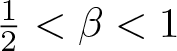 $\frac 12 \lt \beta \lt 1$).
Theorem 1.1. (Young case)
Let 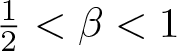 $\frac 12 \lt \beta \lt 1$ and
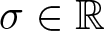 $\sigma \in \mathbb{R}$ satisfy
 \begin{equation}
\sigma \gt - 2 \beta + 1.
\end{equation}
Then, there exists small  $s \gt 0$ such that, given
 $\phi \in \operatorname{HS}(L^2(\mathbb{T}); H^\sigma(\mathbb{T}))$, the stochastic heat equation (1.1) is pathwise globally well-posed in
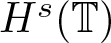 $H^s(\mathbb{T})$.
Following [Reference Gubinelli and Tindel19, Section 4], we define the first-order driver  $\mathbf{X}^1$ by setting
 \begin{equation}
\mathbf{X}^1_{t, r}(f) = \int_r^t
S(t- t') \big[ (S(t' - r) f)
\phi dW^\beta(t') \big]
\end{equation}
for 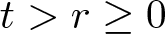 $t \gt r \ge 0$, where
 $f$ is a function on
 $\mathbb{T}$. Then, we make sense of the stochastic convolution
 $\Psi(u)$ in (1.4) as the convolution Young integral
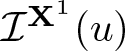 $\mathcal{I}^{\mathbf{X}^1}(u)$ with the first-order driver
 $\mathbf{X}^1$; see §4.1. This allows us to rewrite the Duhamel formulation (1.3) as the following convolution Young differential equation (YDE):
 \begin{equation}
u(t) = S(t) u_0 + \mathcal{I}^{\mathbf{X}^1}(u)(t)
\end{equation}
whose global well-posedness is established in a pathwise manner in §4.3.
The main task is then to construct the convolution Young integral 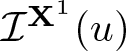 $\mathcal{I}^{\mathbf{X}^1}(u)$. In doing so, we follow the incremental formulation as in [Reference Gubinelli15, Reference Gubinelli and Tindel19], where the matter is reduced to establishing almost sure regularity properties of the random driver
 $\mathbf{X}^1$. In [Reference Gubinelli and Tindel19], Gubinelli and Tindel estimated the operator norm of
 $\mathbf{X}^1$ by its Hilbert–Schmidt norm, which led to a loss. In our novel approach, we study regularity properties of
 $\mathbf{X}^1$ by applying the random tensor estimate for (multiple) stochastic integrals (Lemma 3.5), developed in [Reference Chapouto, Li and Oh5, Reference Chapouto, Li, Oh and Zheng7, Reference Oh, Wang and Zine30]; see § 4.2. A primary reason for working with the Hilbert–Schmidt norm in [Reference Gubinelli and Tindel19] (which may be viewed as the
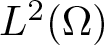
 $\ell^2$-norm for eigenvalues in some setting) is its compatibility with the Wiener–Ito isometry (related to the
 $L^2(\Omega)$-norm). On the other hand, the operator norm may be regarded as the
 $\ell^\infty$-norm, which is not compatible with the
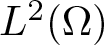 $L^2(\Omega)$-norm for the Wiener–Ito isometry. The main idea behind the random tensor estimate, due to Deng, Nahmod, and Yue [Reference Deng, Nahmod and Yue12], is as follows; instead of working with the Hilbert–Schmidt norm of a random operator (
 $\mathbf{X}^1$ in our setting), we work with the Hilbert–Schmidt norm (= the
 $\ell^2$-norm) of a very high power of
 $\mathbf{X}^1$, say the
 $k$th power. This gives a control on the
 $\ell^{2k}$-norm of (the kernel of)
 $\mathbf{X}^1$, providing a good approximation for the
 $\ell^\infty$-norm (= the operator norm) when
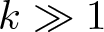 $k \gg 1$, which is far more effective than approximating the
 $\ell^\infty$-norm by the
 $\ell^2$-norm. In the proof of the random tensor estimate, the kernel of a high power of
 $\mathbf{X}^1$ is estimated in an inductive manner. We point out that the Wiener chaos estimate (Lemma 3.2) plays a crucial role in reducing the matter to estimating the Hilbert–Schmidt norm of a high power of
 $\mathbf{X}^1$ (more precisely, the
 $\ell^2$-norm of the kernel of a high power of
 $\mathbf{X}^1$); see [Reference Chapouto, Li and Oh5, Reference Oh, Wang and Zine30] for the proofs. We note that a precursor of this idea (of working with a higher power of a random operator) already appears in a seminal work [Reference Bourgain1] by Bourgain. See also Remark 3.6. Lastly, we remark that, as pointed out in [Reference Bringmann3, Remark 6.6], the random tensor estimate is closely related to operator bounds for structured random matrices and can be proven using the non-commutative Khintchine inequality [Reference van Handel32, Theorem 3.2]. See [Reference Bringmann3, Reference Kaneshiro22] for a further discussion.
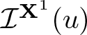
Once we establish almost sure regularity properties of the driver  $\mathbf{X}^1$ (Proposition 4.2), we can simply apply the convolution sewing lemma (Lemma 4.1) to construct the convolution Young integral
 $\mathcal{I}^{\mathbf{X}^1}(u)$ in a pathwise manner. We note that local well-posedness of the convolution YDE (1.12) then follows from a standard contraction argument, whereas its global well-posedness follows from an iterative application of the local well-posedness argument.
Remark 1.2. In [Reference Gubinelli and Tindel19, Theorem 4.12], Gubinelli and Tindel studied the case 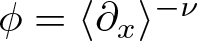 $\phi = \langle \partial_x \rangle^{-\nu}$,
 $0 \le \nu \lt 1$, which belongs to
 $\operatorname{HS}(L^2(\mathbb{T}); H^\sigma(\mathbb{T}))$ if and only if
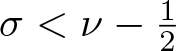 $\sigma \lt \nu - \frac 12$. In this setting, the condition (1.10) in Theorem 1.1 reduces to
 \begin{equation}
\nu \gt - 2 \beta + \frac 32.
\end{equation}
Compare this with the condition in [Reference Gubinelli and Tindel19, Remark 4.9]:
 \begin{equation}
\nu \gt - 4\beta +3.
\end{equation}
Recalling that  $\nu \ge 0$, our condition (1.13) provides an improvement over the condition (1.14) from [Reference Gubinelli and Tindel19] (restricted to
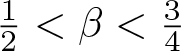 $\frac 12 \lt \beta \lt \frac 34$; for
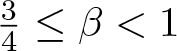 $\frac 34 \le \beta \lt 1$, both (1.13) and (1.14) provide the same conclusion under the restriction
 $\nu \ge 0$).
Next, we state a pathwise well-posedness result in the rough case (= the white-in-time case with the Hurst parameter 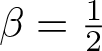 $\beta = \frac 12$) in a somewhat formal manner.
Theorem 1.3. (rough case)
Let 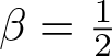 $\beta = \frac 12$ and
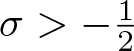 $\sigma \gt - \frac 12$. Then, there exists small
 $s \gt 0$ such that, given
 $\phi \in \operatorname{HS}(L^2(\mathbb{T}); H^\sigma(\mathbb{T}))$, the stochastic heat equation (1.1) is pathwise globally well-posed in
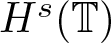 $H^s(\mathbb{T})$.
Following [Reference Gubinelli and Tindel19, Section 5], we introduce the second-order driver  $\mathbf{X}^2$ and the third-order driver
 $\mathbf{X}^3$ via the recursive relation (5.1) (see also (5.2)); see (5.20) and (5.21) for direct definitions of
 $\mathbf{X}^2$ and
 $\mathbf{X}^3$, respectively. Then, we make sense of the stochastic convolution
 $\Psi(u)$ in (1.4) as the convolution rough integral
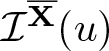 $\mathcal{I}^{\overline{\mathbf{X}}}(u)$ with the driver
 $\overline{\mathbf{X}} = (\mathbf{X}^1, \mathbf{X}^2, \mathbf{X}^3)$ by imposing a second-order controlled structure on
 $u$; see §5.1. This allows us to rewrite the Duhamel formulation (1.3) as the following convolution rough differential equation (RDE):
 \begin{align*}
u(t) = S(t) u_0 + \mathcal{I}^{\overline{\mathbf{X}}}(u)(t).
\end{align*}
Once the convolution rough integral 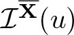 $\mathcal{I}^{\overline{\mathbf{X}}}(u)$ is constructed in a suitable manner, a standard contraction with the second-order controlled structure on the unknown
 $u$ yields local and global well-posedness in a pathwise manner; see §5.3.
As in the Young case, the main task in constructing the convolution rough integral 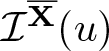 $\mathcal{I}^{\overline{\mathbf{X}}}(u)$ with the driver
 $\overline{\mathbf{X}} = (\mathbf{X}^1, \mathbf{X}^2, \mathbf{X}^3)$ is to establish almost sure regularity properties of the higher-order drivers
 $\mathbf{X}^2$ and
 $\mathbf{X}^3$. We achieve this by applying the random tensor estimate and arguing inductively (see (5.41) and (5.59)) by exploiting the smoothing property of the heat semigroup
 $S(t)$ (on the Fourier side). See §5.2.
Remark 1.4. Recall that the case of a space-time white noise corresponds to 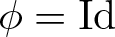 $\phi = \operatorname{Id}$, which belongs to
 $ \operatorname{HS}(L^2(\mathbb{T}); H^\sigma(\mathbb{T}))$ for
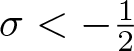 $\sigma \lt - \frac 12$. Theorem 1.3 provides the condition
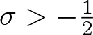 $\sigma \gt - \frac 12$, thus allowing us to treat an almost space-time white noise, for example,
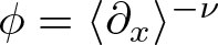 $\phi = \langle \partial_x \rangle^{-\nu}$ for any
 $\nu \gt 0$. This yields a significant improvement over [Reference Gubinelli and Tindel19], where the condition
 $\nu \gt \frac 13$ was obtained via the same third-order expansion as explained above.
We also note that Theorem 1.3 is optimal in the following sense. When 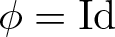 $\phi = \operatorname{Id}$ (with
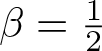 $\beta = \frac 12$), the noise
 $\zeta$ in (1.1) corresponds to the space-time white noise
 $\xi$ whose temporal and spatial regularities are
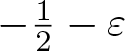 $-\frac 12- \varepsilon$,
 $\varepsilon \gt 0$, almost surely. In this case, the stochastic convolution
 $\Psi$ (with
 $u \equiv1$), given by
 \begin{align*}
\Psi(t) =
\int_0^t S(t-t') \phi dW^\beta (t'),
\end{align*}
has temporal and spatial regularities  $\frac 12- \varepsilon$,
 $\varepsilon \gt 0$, almost surely. In studying (1.1), we need to understand the formal product
 $\Psi \xi$ as the first approximation. However, this formal product suffers the deficiency of regularity in both temporal and spatial directions. Namely, the sum of regularities is negative in both temporal and spatial directions. As such, the standard one-parameter rough path theory is not sufficient to treat this problem and one needs to carry out bi-parameter analysis as in [Reference Chouk and Gubinelli8]. We will address this problem in a forthcoming work.
Lastly, we point out that the theory of regularity structures, introduced by Hairer [Reference Hairer20], allows us to prove the well-posedness of (1.1) in the case of a space-time white noise, since it treats temporal and spatial regularities in a unified manner (called homogeneity), thus avoiding the necessity of bi-parameter analysis. See [Reference Hairer and Pardoux21].
Remark 1.5. (i) For simplicity of presentation, we restricted our attention to the one-dimensional case, but our analysis can be easily adapted to higher dimensions, improving the corresponding results in [Reference Gubinelli and Tindel19]. By the same reason, we only considered the noise of the form  $u \phi \zeta$ in this paper, but our approach can be easily adapted to treat the noise of the form
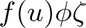 $f(u) \phi \zeta$ in the Young case under a suitable assumption on
 $f(u)$. In [Reference Gubinelli and Tindel19, Section 6], Gubinelli and Tindel studied the noise of the form
 $u^2 \phi \xi$ in the rough case, using nonlinear rough path analysis as in [Reference Gubinelli16]; see also [Reference Nualart and Xia26, Reference Oh and Shao27]. In a forthcoming work, we will revisit this problem using the random tensor approach.
(ii) In this paper, we study the first-, second-, and third-order drivers  $\mathbf{X}^1$,
 $\mathbf{X}^2$, and
 $\mathbf{X}^3$ for
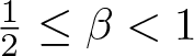 $\frac 12 \le \beta \lt 1$ via the random tensor estimates; see Propositions 4.2, 5.2, and 5.3. As mentioned above, our argument is inductive and thus can be easily adapted to treat a higher-order driver
 $\mathbf{X}^j$ of an arbitrary degree, defined by the recursive relation (5.2). It may be of interest to improve the regularity condition on
 $\phi$ in the Young case by considering a sufficiently higher-order expansion. See also Remark 4.3. We, however, do not pursue this issue further in this paper.
2. Notations and function spaces
2.1. Basic notations
We use 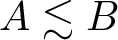 $A\lesssim B$ to denote an estimate of the form
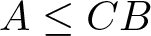 $A\leq CB$ for some constant
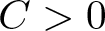 $C \gt 0$. We write
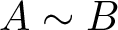 $A\sim B$ if
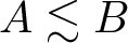 $A\lesssim B$ and
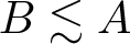 $B\lesssim A$, while
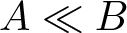 $A\ll B$ denotes
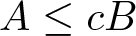 $A\leq c B$ for some small constant
 $c \gt 0$. We may write
 $\lesssim_{\alpha}$ and
 $\sim_{\alpha}$ to emphasize the dependence on an external parameter
 $\alpha$. We use
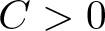 $C \gt 0$ to denote various constants, which may vary line by line, and we write
 $C_{\alpha}$ to emphasize the dependence on an external parameter
 $\alpha$.
Given 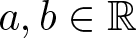 $a, b \in \mathbb{R}$, we set
 $a\vee b = \max(a, b)$ and
 $a\wedge b = \min(a, b)$.
In expressing the dependence of a function  $u$ on the time variable, we often use the short-hand notation
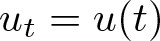 $u_t = u(t)$, which is standard in probability theory and stochastic analysis. Similarly, we often use the short-hand notation
 $S_t$ for the heat semigroup
 $S(t) = e^{t(\Delta - 1)}$. In considering an integral (in time) operator
 $\mathcal{I}$, a priori defined on functions on
 $\mathbb{T}$, we use the notation
 $\mathcal{I}(u_\bullet)$ to denote its (formal) action on a space-time function
 $u$, where
 $\bullet$ denotes the variable of integration. For example, by comparing (1.4) and (4.2), we have
 \begin{equation*} \Psi(u)(t) = \mathbf{Y}_{t, 0}(u_{\bullet}),\end{equation*}
where the right-hand side is merely a formal expression.
Given  $n_{j_1}, \dots, n_{j_k} \in \mathbb{Z}$, we set
 \begin{equation}
n_{j_1 \cdots j_k} =
n_{j_1}+ \cdots+ n_{j_k}.
\end{equation}
For example,  $n_{123} = n_1 + n_2 + n_3$.
We set  $\mathbb{Z}_{\ge 0} = \mathbb{N} \cup\{0\}$ and use
 $2^{\mathbb{Z}_{\ge 0}}$ to denote the set of dyadic numbers
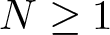 $N\ge 1$.
2.2. Function spaces
By convention, we endow  $\mathbb{T}$ with the normalized Lebesgue measure
 $ dx_{\mathbb{T}} = (2\pi)^{-1}dx$ such that we do not need to carry factors involving
 $2\pi$. Given
 $s \in \mathbb{R}$, let
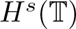 $H^s(\mathbb{T})$ be the
 $L^2$-based Sobolev space defined by the norm:
 \begin{equation*} \| f\|_{H^s} = \bigg(\sum_{n \in \mathbb{Z}} \langle n \rangle^{2s} |\widehat f(n)|^2\bigg)^\frac 12, \end{equation*}
where  $\widehat f$ denotes the Fourier transform of
 $f$.
In studying space-time functions, we often use short-hand notations such as  $L^\infty_T H^s_x = L^\infty([0, T]; H^s(\mathbb{T}))$, etc. when there is no ambiguity.
Given Banach spaces  $V$ and
 $W$, we use
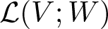 $\mathcal{L}(V; W)$ to denote the Banach space of bounded linear operators from
 $V$ to
 $W$. When
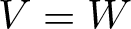 $V = W$, we simply set
 $\mathcal{L}(V) = \mathcal{L}(V;V)$.
Let  $V$ be a Banach space and
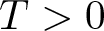 $T \gt 0$. For
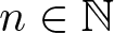 $n\in\mathbb{N}$, we set
 \begin{align*}
\Delta_{n, T} =
\big\{(t_1, \ldots, t_n) \in [0,T]^n: \ t_i \gt t_j
\text{for } i \lt j\big\}.
\end{align*}
We denote by 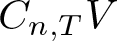 $C_{n,T}V$ the space of continuous functions from
 $\Delta_{n,T}$ to
 $V$. When
 $n=1$, we may write
 $C_T V$ for simplicity and equip this space with the supremum norm:
 \begin{align*}
\|f\|_{C_T V} = \|f\|_{L^\infty_T V} = \sup_{0\leq t \leq T} \|f(t)\|_V.
\end{align*}
We define the coboundary operator  ${\delta}: C_{n,T} V \to C_{n+1,T} V$ as follows; given
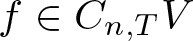 $f\in C_{n,T} V$ and
 $(t_1,\ldots, t_{n+1}) \in \Delta_{{n+1},T}$, we set
 \begin{align*}
({\delta} f)_{t_1,\ldots , t_{n+1}} =
\sum_{k=1}^{n+1} (-1)^{k} f_{t_1, \ldots, t_{k-1}, t_{k+1}, \ldots, t_{n+1}}.
\end{align*}
For example, for 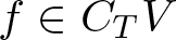 $f\in C_T V$ and
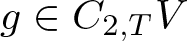 $g\in C_{2,T} V$, we have
 \begin{align}
({\delta} f )_{t,r} &= f_t - f_r, \cr
({\delta} g)_{t_1,t_2,t_3} &=
g_{t_1,t_3} - g_{t_1,t_2} - g_{t_2,t_3}
\end{align}
for  $(t,r)\in\Delta_{2,T}$ and
 $(t_1,t_2,t_3) \in \Delta_{3,T}$. As noted in [Reference Gubinelli and Tindel19], the sequence
 \begin{align*}
0 \longrightarrow {V} \longrightarrow C_{1, T}V \stackrel{{\delta}}{\longrightarrow} C_{2, T}V
\stackrel{{\delta}}{\longrightarrow} C_{3, T}V
\stackrel{{\delta}}{\longrightarrow} \cdots
\end{align*}
is exact. In particular, we have  ${\delta}\circ{\delta} =0$ and if
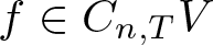 $f \in C_{n,T} V$ with
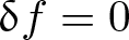 ${\delta} f =0$, then there exists a
 $g\in C_{n-1,T}V$ such that
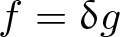 $f= {\delta} g$; see, for example, [Reference Gubinelli and Tindel19, Lemma 2.1].
In the following, we go over a similar complex structure in the convolution setting; see [Reference Gubinelli and Tindel19, Section 3]. Let 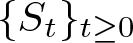 $\{S_t\}_{t\ge 0}$ be a semigroup of bounded operators on a separable Banach space
 $V$ with
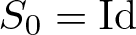 $S_0 = \operatorname{Id}$, satisfying
 \begin{equation}
\|S_t f\|_{V} \le \|f\|_V.
\end{equation}
We then set
 \begin{equation}
A_{t} = S_{t} - \operatorname{Id}.
\end{equation}
We now define the convolution coboundary operator  $\widehat {\delta}$ by
 \begin{align*}
(\widehat {\delta} f)_{t_1,\ldots , t_{n+1}}
= ( {\delta} f)_{t_1,\ldots , t_{n+1}}
- A_{t_1 - t_2}
f_{t_2,\ldots , t_{n+1}}
\end{align*}
for 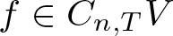 $f \in C_{n, T}V$ and
 $(t_1,\ldots, t_{n+1}) \in \Delta_{{n+1},T}$. For example, for
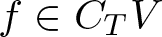 $f\in C_T V$ and
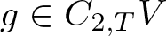 $g\in C_{2,T} V$, we have
 \begin{align}
(\widehat{ {\delta}} f)_{t, r}
& = ({\delta} f)_{t, r} - A_{t-r} f_r
= f_t - S_{t-r} f_r, \cr
(\widehat {{\delta}} g)_{t_1, t_2, t_3}
& =
g_{t_1, t_3}
- g_{t_1, t_2}
- S_{t_1-t_2}g_{t_2, t_3}
\end{align}
for  $(t,r)\in\Delta_{2,T}$ and
 $(t_1,t_2,t_3) \in \Delta_{3,T}$, where
 ${\delta}$ is as in (2.2). Compare (2.5) with (2.2). Then, as in the non-convolution setting, the sequence
 \begin{align*}
0 \longrightarrow {S_t}{V} \longrightarrow C_{1, T}V \stackrel{\widehat {{\delta}}}
{\longrightarrow} C_{2, T}V
\stackrel{\widehat {{\delta}}}{\longrightarrow} C_{3, T}V
\stackrel{\widehat {{\delta}}}{\longrightarrow} \cdots
\end{align*}
is exact, where  ${{S_t} V}$ denotes the space of “linear solutions”:
 \begin{align*} S_t V = \{S_t v : v \in V\}.\end{align*}
In particular, we have 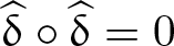 $\widehat {\delta}\circ\widehat {\delta} =0$ and if
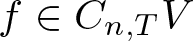 $f \in C_{n,T} V$ with
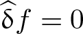 $\widehat {\delta} f =0$, then there exists a
 $g\in C_{n-1,T}V$ such that
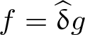 $f= \widehat {\delta} g$; see [Reference Gubinelli and Tindel19, Proposition 3.1].
We also define an auxiliary operator  $\widetilde {\delta}$, acting on operator-valued increments
 $X \in C_{2, T} \mathcal{L}(V)$, by setting
 \begin{align}
(\widetilde{{\delta}} X)_{t_1, t_2, t_3}
& = (\widehat {{\delta}} X)_{t_1, t_2, t_3} - X_{t_1, t_2}A_{t_2 - t_3}\cr
& = ({\delta} X)_{t_1, t_2, t_3} - A_{t_1 - t_2} X_{t_2, t_3}
- X_{t_1, t_2}A_{t_2 - t_3}
\end{align}
for  $(t_1,t_2,t_3) \in \Delta_{3,T}$, where
 $A$ is as in (2.4). The operator
 $\widetilde {\delta}$ allows us to express Chen’s relation in the current convolution setting in a concise manner; see (4.5), (5.3), and (5.7). See also (2.8) below.
Given  $X \in C_{n, T}\mathcal{L}(V)$ and
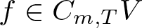 $f \in C_{m, T}V$, we define their contraction
 $X(f) \in C_{n+m - 1, T}V$ by
 \begin{equation}
\big(X(f)\big)_{t_1, \dots, t_{n+m-1}} =
X_{t_1, \dots, t_n}
( f_{t_n, \dots, t_{n+m-1}})
\end{equation}
for  $(t_1, \dots, t_n)\in \Delta_{n, T}$ and
 $(t_n, \dots, t_{n+m-1}) \in \Delta_{m, T}$. We also recall the following product rule for
 $\widehat {\delta}$ defined in (2.5); given
 $X \in C_{2, T}\mathcal{L}(V)$ and
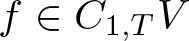 $f \in C_{1, T}V$, we have
 \begin{equation}
\widehat {\delta} (X(f)) = (\widehat {\delta} X)(f) - X({\delta} f)
= (\widetilde {\delta} X)(f) - X(\widehat {\delta} f),
\end{equation}
where  $\widetilde {\delta}$ is as in (2.6) and the right-hand side is understood in the sense of (2.7); see [Reference Gubinelli and Tindel19, math display after (89)], which follows as a variant of [Reference Gubinelli and Tindel19, Lemma 3.2].
For 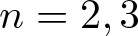 $n = 2, 3$, we introduce the spaces
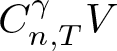 $C^\gamma_{n,T}V$, equipped with the following Hölder-type norms; for
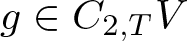 $g\in C_{2,T}V$ and
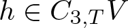 $h\in C_{3,T}V$, we set
 \begin{align}
\| g\|_{C^\gamma_{2,T} V} &
= \sup_{(t,r) \in \Delta_{2,T}} \frac{\|g_{t,r} \|_{V} }{|t-r|^{\gamma}}, \cr
\| h\|_{C^\gamma_{3,T} V} &
= \inf_{0 \lt \alpha \lt \gamma}
\sup_{(t_1,t_2,t_3) \in \Delta_{3,T}}
\frac{\|h_{t_1,t_2,t_3}\|_V}
{|t_1-t_2|^{\alpha} |t_2-t_3|^{\gamma-\alpha}}.
\end{align}
Lastly, we define the class  $\widehat C_{T}^\gamma V$ to be the collection of functions
 $f$ satisfying
 \begin{equation}
\|f \|_{\widehat C_{T}^\gamma V}
= \|\widehat {\delta} f\|_{C^\gamma_{2, T} V}
= \sup_{(t,r)\in \Delta_{2,T}}
\frac{\|(\widehat {\delta} f)_{t,r}\|_V}{|t-r|^\gamma} \lt \infty
\end{equation}
and define  $\widehat{\mathcal{C}}^\gamma_T V = \widehat{\mathcal{C}}^\gamma([0, T]; V)
= \widehat C_{T}^\gamma V\cap L^\infty_T V$ via the norm:
 \begin{equation}
\| f \|_{\widehat{\mathcal{C}}^\gamma_TV} = \| f \|_{L^\infty_TV} + \|f\|_{\widehat C^\gamma_T V}.
\end{equation}
From (2.5), we have  $f_t = (\widehat {\delta} f)_{t, 0}+ S_t f_0$. Thus, from (2.10) and (2.3), we have
 \begin{equation}
\|f\|_{L^\infty_T V} \le T^\gamma \|f\|_{\widehat C^\gamma_T V} + \|f_0\|_{V}.
\end{equation}
3. Random tensor estimate
In this section, we first go over the basic definitions and properties of multiple stochastic integrals with respect to fractional Brownian motions. In §3.2, we state the random tensor estimate (Lemma 3.5), which plays a crucial role in establishing almost sure mapping properties of the drivers  $\mathbf{X}^j$,
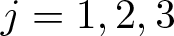 $j = 1, 2, 3$. See §4.2 and §5.2.
3.1. Fractional Brownian motion and multiple stochastic integrals
In this subsection, we briefly go over the basic definitions and properties of fractional Brownian motions and Wiener integrals with respect to fractional Brownian motions. See [Reference Nualart25, Chapter 5] for a further discussion.
Definition 3.1. Let 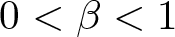 $0 \lt \beta \lt 1$. A (real-valued) fractional Brownian motion
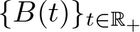 $\{B(t)\}_{t\in \mathbb{R}_+}$ with Hurst parameter
 $\beta$ is a centered Gaussian process with covariance given by
 \begin{align*}
\mathbb{E}[B(t_1) B(t_2)] = \frac12 \Big( t_1^{2\beta} + t_2^{2\beta} - |t_1-t_2|^{2\beta}\Big) .
\end{align*}
When 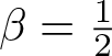 $\beta=\frac12$, this process reduces to the standard Brownian motion. A complex-valued fractional Brownian motion
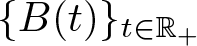 $\{B(t)\}_{t\in \mathbb{R}_+}$ with Hurst parameter
 $\beta$ is a complex-valued centered Gaussian process such that
 $\{\sqrt 2\ {\text{Re}}\ B(t)\}_{t\in \mathbb{R}_+}$ and
 $\{\sqrt 2\ {\text{Im}}\ B(t)\}_{t\in \mathbb{R}_+}$ are independent real-valued fractional Brownian motions with Hurst parameter
 $\beta$ such that
 \begin{equation*} \mathbb{E}\big[ |B(t_1) - B(t_2)|^2\big] = |t_1 - t_2|^{2\beta}.\end{equation*}
See also [Reference Oh, Sosoe and Tzvetkov28, Section 5] for a discussion on fractional Brownian motions.
Let us first introduce the following partition of  $\mathbb{Z}^d$:
 \begin{align*}
\mathbb{Z}^d = (\mathbb{Z}^d)_+ \cup (\mathbb{Z}^d)_- \cup \{0\}^d ,
\end{align*}
where
 \begin{equation*}
(\mathbb{Z}^d)_+=\bigcup_{k=0}^{d-1} \mathbb{Z}^k\times \mathbb{Z}_{+}\times \{0\}^{d-k-1}
\qquad \text{and}\qquad
(\mathbb{Z}^d)_- = -(\mathbb{Z}^d)_+.
\end{equation*}
Given 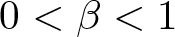 $0 \lt \beta \lt 1$, let
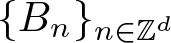
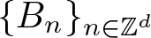 $\{B_n\}_{n\in \mathbb{Z}^d}$ be a family of mutually independent complex-valued fractional Brownian motions with Hurst parameter
 $\beta$, conditioned that
 \begin{equation}
B_{-n} = \overline{B_n}, \qquad n \in \mathbb{Z}^d,
\end{equation}
which in particular implies that  $B_0$ is real-valued. Then,
 $\{B_0\}\cup \{\sqrt 2\ {\text{Re}}\ B_n, \sqrt 2\ {\text{Im}}\ B_n \}_{n\in (\mathbb{Z}^d)_{+}}$ forms a family of mutually independent real-valued fractional Brownian motions with the same Hurst parameter
 $\beta$.
In order to define stochastic integrals with respect to these fractional Brownian motions, we need the following real Hilbert space. For 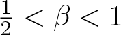 $\frac 12 \lt \beta \lt 1$, let
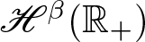 $\mathscr{H}^\beta(\mathbb{R}_+)$ be the completion of linear combinations of (real-valued) step functions on
 $\mathbb{R}_+$ under the following norm:
 \begin{align}
\|f\|_{\mathscr{H}^\beta(\mathbb{R}_+)}^2 &= \beta(2\beta-1) \int_0^\infty \int_0^\infty f(t) f(t') |t-t'|^{2\beta-2}\, dt\, dt' \nonumber\\
& = C_\beta \int_0^\infty f(t)\,\mathfrak{I}_{2\beta-1}(f)(t)\, dt \nonumber\\
& = C_\beta \int_{\mathbb{R}} |\tau|^{1-2\beta} |\widehat{f}(\tau)|^2\, d\tau \nonumber\\
& = C_\beta \|f\|_{\dot H^{\frac12-\beta}(\mathbb{R})}^2
\end{align}
for a function  $f$ supported on
 $\mathbb{R}_+$, where
 $\mathfrak{I}_{2\beta-1} = |\partial_t|^{1-2\beta}$ denotes the Riesz potential of order
 $2\beta - 1 \gt 0$. Note that on the class of functions
 $f$ on
 $\mathbb{R}$ with
 $\mathrm{supp} (f) \subset \mathbb{R}_+$, (3.2) defines a norm, not a semi-norm. Similarly, given
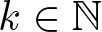 $k \in \mathbb{N}$, we define
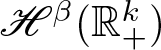 $\mathscr{H}^\beta(\mathbb{R}_+^k)$ (with the understanding that
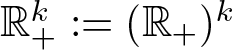 $\mathbb{R}_+^k := (\mathbb{R}_+)^k$) to be the completion of linear combinations of products of step functions in
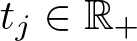 $t_j \in \mathbb{R}_+$,
 $j = 1, \dots, k$, under
 \begin{align}
\|f\|_{\mathscr{H}^\beta(\mathbb{R}_+^k)}^2
& = \beta^k(2\beta-1)^k
\int_{\mathbb{R}_+^{2k}}
f(t_1, \dots, t_k)
f(t_1', \dots, t_k')
\prod_{j = 1}^k |t_j-t_j'|^{2\beta-2} dt_jdt_j' \cr
&= C_\beta^k
\bigg\| \prod_{j = 1}^k |\partial_{t_j}|^{\frac 12 - \beta}f\bigg\|_{L^2(\mathbb{R}^k_+)}^2
\end{align}
for a function  $f(t_1, \dots, t_k)$ supported on
 $\mathbb{R}_+^k$. When
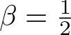 $\beta = \frac12$, we set
 \begin{equation}
\mathscr{H}^\frac12(\mathbb{R}^k_+) = L^2(\mathbb{R}_+^k).
\end{equation}
We say that a sequence  $f = \{f_n \}_{n \in \mathbb{Z}^d}$ of complex-valued functions
 $f_n$ on
 $\mathbb{R}_+$ belongs to
 $ \ell^2(\mathbb{Z}^d;\mathscr{H}^\beta(\mathbb{R}_+))$, if we have
 \begin{equation}
f_{-n} = \overline{f_n}, \quad n \in \mathbb{Z}^d,
\end{equation}
and  ${\text{Re}}\ f_n, {\text{Im}}\ f_n \in \mathscr{H}^\beta(\mathbb{R}_+)$ (note from (3.5) that
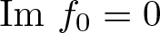 ${\text{Im}}\ f_0 = 0$) such that
 \begin{align*}
\|f\|_{\ell^2(\mathbb{Z}^d;\mathscr{H}^\beta(\mathbb{R}_+))}
:\! & = \bigg(\sum_{n \in \mathbb{Z}^d} \| f_n\|_{\mathscr{H}^\beta(\mathbb{R}_+)}^2\bigg)^\frac 12\\
& = \bigg(\sum_{n \in \mathbb{Z}^d} \|\ {\text{Re}}\ f_n\|_{\mathscr{H}^\beta(\mathbb{R}_+)}^2
+ \sum_{n \in \mathbb{Z}^d} \|\ {\text{Im}}\ f_n\|_{\mathscr{H}^\beta(\mathbb{R}_+)}^2\bigg)^\frac 12 \lt \infty.
\end{align*}
We then define the Wiener integral of  $f$ with respect to
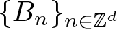 $\{B_n\}_{n\in\mathbb{Z}^d}$ by setting
 \begin{align}
I_1[f]
& = \sum_{n\in \mathbb{Z}^d}J_n^{(r)}(f_n)
+ \sum_{n\in \mathbb{Z}^d}J_n^{(i)}(f_n)\cr
& = \sum_{n\in \mathbb{Z}^d} \int _0^\infty f_n(t) d\, {\text{Re}}\ B_n(t)
+ i
\sum_{n\in \mathbb{Z}^d}
\int _0^\infty f_n(t) d\, {\text{Im}}\ B_n(t).\cr
\end{align}
Note that  $I_1[f]$ is real-valued in view of the conditions (3.1) and (3.5). In (3.6), each summand
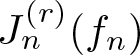 $J_n^{(r)}(f_n)$ or
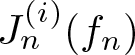 $J_n^{(i)}(f_n)$ is understood as a Wiener integral; namely,
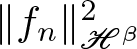
 $\{J_0^{(r)}(f_0)\}\cup \{\sqrt{2}J_n^{(r)}(f_n), \sqrt{2}J_n^{(i)}(f_n)\}_{n \in (\mathbb{Z}^d)_{+}}$ is a family of independent mean-zero Gaussian random variables with variance
 $\|f_n\|_{\mathscr{H}^\beta}^2$. In particular, the map
 $I_1$ is an isometry from
 $\ell^2(\mathbb{Z}^d;\mathscr{H}^\beta(\mathbb{R}_+))$ into
 $L^2(\Omega, \sigma(I_1) , \mathbb{P})$, where
 $\sigma(I_1)$ is the
 $\sigma$-algebra generated by the process
 $I_1= \{I_1[f]: f \in \ell^2(\mathbb{Z}^d;\mathscr{H}^\beta(\mathbb{R}_+))\}$. (Here, we view
 $I_1$ as a process indexed by
 $f \in \ell^2(\mathbb{Z}^d;\mathscr{H}^\beta(\mathbb{R}_+))$.) The process
 $I_1$ is known as an isonormal Gaussian process associated with the Hilbert space
 $\ell^2(\mathbb{Z}^d;\mathscr{H}^\beta(\mathbb{R}_+))$, satisfying
 \begin{align*}
\mathbb{E}\big[I_1[f] I_1[g]\big] = \langle f,g \rangle_{\ell^2_n \mathscr{H}_t^\beta }
\end{align*}
for any  $f,g\in
\ell^2(\mathbb{Z}^d;\mathscr{H}^\beta(\mathbb{R}_+))$; see [Reference Nualart25, Definition 1.1.1].
Given 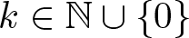 $k \in \mathbb{N} \cup\{0\}$, we define the
 $k$th homogeneous Wiener chaos
 $\mathcal{H}_k$ to be the closed linear subspace of
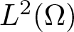 $L^2(\Omega)$ generated by
 \begin{align*}
\big\{H_k(I_1[f]) : \, f\in \ell^2(\mathbb{Z}^d;\mathscr{H}^\beta(\mathbb{R}_+)), \, \|f\|_{\ell^2_n\mathscr{H}^\beta_t} = 1 \big\},
\end{align*}
where  $H_k$ denotes the Hermite polynomial of degree
 $k$, defined via the following generating function:
 \begin{equation*}
e^{tx - \frac{1}{2} t^2} = \sum_{k = 0}^\infty \frac{t^k}{k!} H_k(x).
\end{equation*}
For readers’ convenience, we write out the first few Hermite polynomials:
 \begin{align*}
& H_0(x) = 1,
\quad
H_1(x) = x,
\quad
H_2(x) = x^2 - 1,
\quad
H_3(x) = x^3 - 3 x.
\end{align*}
The spaces  $\mathcal{H}_k$ and
 $\mathcal{H}_j$ are orthogonal when
 $k\neq j$, and the real Hilbert space
 $L^2(\Omega, \sigma(I_1), \mathbb{P})$ admits the following Wiener–Ito decomposition:
 \begin{align*}
L^2(\Omega, \sigma(I_1), \mathbb{P}) = \bigoplus_{k=0}^\infty \mathcal{H}_k.
\end{align*}
Note that given any  $f\in \ell^2(\mathbb{Z}^d;\mathscr{H}^\beta(\mathbb{R}_+))$, the stochastic integral
 $I_1[f]$ is an element of the first homogeneous Wiener chaos
 $\mathcal{H}_1$. We now state the Wiener chaos estimate, which follows from the hypercontractivity of the Ornstein–Uhlenbeck semigroup due to Nelson [Reference Nelson24]; see [Reference Simon31, Theorem I.22].
Lemma 3.2. (Wiener chaos estimate)
Let 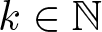 $k\in\mathbb{N}$. Then, given any finite
 $p \ge 1$ and
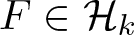 $F \in \mathcal{H}_k$, we have
 \begin{align*}
\| F \|_{L^p(\Omega)} \le p^{\frac k 2 } \| F \|_{L^2(\Omega)}.
\end{align*}
Lastly, we introduce multiple stochastic integrals with respect to the fractional Brownian motions 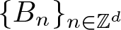 $\{B_n\}_{n\in\mathbb{Z}^d}$ with Hurst parameter
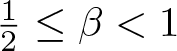 $\frac 12 \le \beta \lt 1$, satisfying (3.1). Fix an integer
 $k \ge 2$. Given
 $f\in \ell^2_{n}( (\mathbb{Z}^d)^{k} ; \mathscr{H}^\beta(\mathbb{R}_+^{k}) )$, where
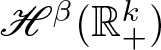 $\mathscr{H}^\beta(\mathbb{R}_+^{k})$ is as in (3.3) and (3.4), we define its symmetrization by
 \begin{align*}
{\texttt{Sym}}(f) (z_1, \ldots, z_k)
= \frac{1}{k!} \sum_{\sigma\in \mathcal{S}_k} f(z_{\sigma(1)}, \ldots, z_{\sigma(k)}),
\end{align*}
where 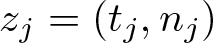 $z_j = (t_j, n_j)$ and
 $\mathcal{S}_k$ denotes the symmetric group on
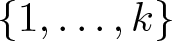 $\{1, \dots, k\}$. We denote by
 $\bigl(\ell^2(({\mathbb{Z}^d})^k; \mathscr{H}^\beta(\mathbb{R}_+^k))\bigr)^\mathrm{Sym}$ the subspace of symmetric functions in
 $(\ell^2(({\mathbb{Z}^d})^k; \mathscr{H}^\beta(\mathbb{R}_+^k))$.
We now introduce the notion of a multiple Wiener integral  $I_k$.
Definition 3.3. Let 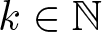 $k\in\mathbb{N}$. The
 $k$th multiple Wiener integral
 $I_k$ is an isometry (up to a constant factor; see (3.7)) from
 $\bigl(\ell^2( (\mathbb{Z}^d)^{k} ; \mathscr{H}^\beta(\mathbb{R}_+^{k}))\bigr)^{\mathrm{Sym}}$ into the Wiener chaos
 $\mathcal{H}_k$, uniquely determined by
 \begin{align*}
I_k[ h_1^{\otimes k_1} \otimes \cdots \otimes h_n^{\otimes k_n} ] = \prod_{j=1}^n H_{k_j} (I_1[h_j])
\end{align*}
for any orthonormal elements  $h_1, \ldots, h_n \in
\ell^2(\mathbb{Z}^d;\mathscr{H}^\beta(\mathbb{R}_+))$ and
 $k_1, \dots, k_n \in \mathbb{N}\cup\{0\}$ such that
 $k = k_1 + \ldots + k_n$, where
 $H_{k}$ denotes the Hermite polynomial of degree
 $k$ and
 $I_1$ is as in (3.6).
• For general (possibly non-symmetric)
 $f\in
\ell^2( (\mathbb{Z}^d)^{k} ; \mathscr{H}^\beta(\mathbb{R}_+^{k}) )$, we set
\begin{align*}I_k[f] = I_k [ {\texttt{Sym}}(f)].\end{align*}
• Given
$f\in
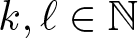
\ell^2( (\mathbb{Z}^d)^{k} ; \mathscr{H}^\beta(\mathbb{R}_+^{k}) )$ and $g\in \ell^2( (\mathbb{Z}^d)^\ell ; \mathscr{H}^\beta(\mathbb{R}_+^{\ell}) )$ for some $k, \ell \in \mathbb{N}$, we have
where\begin{align*}
\mathbb{E} \big[ I_k[f] I_\ell[g] \big] = k! \cdot \mathbf 1_{k=\ell} \cdot \langle {\texttt{Sym}}(f), {\texttt{Sym}}(g) \rangle_{\ell^2_{n_1, \dots, n_k} \mathscr{H}^\beta_{t_1, \dots, t_k}},
\end{align*}
$\ell^2_{n_1, \dots, n_k} \mathscr{H}^\beta_{t_1, \dots, t_k}$ is a short-hand notation for $\ell^2( (\mathbb{Z}^d)^{k} ; \mathscr{H}^\beta(\mathbb{R}_+^{k}) )$.• When
$\beta=\frac{1}{2}$, the multiple Wiener integrals agree with the iterated Wiener–Ito integrals with respect to a family $\{B_n \}_{n \in \mathbb{Z}^d}$ of mutually independent standard Brownian motions, satisfying (3.1). Furthermore, suppose that $f$ is symmetric. Then, we have
where\begin{align*}
& I_k[f]
= k! \sum_{n_1, \cdots, n_k \in \mathbb{Z}^d}
\int_{\Delta_k}
f(t_1, n_1, \dots, t_k, n_k)
dB_{n_k}(t_k) \cdots dB_{n_1}(t_1),
\end{align*}
$\Delta_k
= \big\{(t_1, \ldots, t_k) \in \mathbb{R}_+^k: \ t_i \gt t_j\ \text{for}\ i \lt j\big\}$. Here, the iterated integral on the right-hand side is understood as an iterated Ito integral; see [Reference Nualart25, p. 23].










3.2. Random tensor estimate
In this subsection, we provide the basic definition of tensors and state the random tensor estimate (Lemma 3.5). See [Reference Deng, Nahmod and Yue12, Sections 2 and 4], [Reference Bringmann2, Section 4], [Reference Oh, Wang and Zine30, Appendix C], and [Reference Oh and Wang29, Section 2] for further discussions.
Definition 3.4. Let  $A$ be a finite index set. We denote by
 $n_A$ the tuple
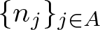 $ \{n_j \}_{j \in A}$. A tensor
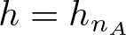 $h = h_{n_A}$ is a function:
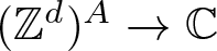 $(\mathbb{Z}^d)^{A} \to \mathbb{C} $ with the input variables
 $n_A$. Note that the tensor
 $h$ may also depend on
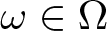 $\omega \in \Omega$. The support of a tensor
 $h$ is the set of
 $n_A$ such that
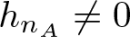 $h_{n_A} \neq 0$.
Given a finite index set  $A$, let
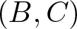 $(B, C)$ be a partition of
 $A$. We define the norms
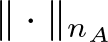 $\| \cdot \|_{n_A}$ and
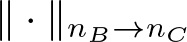 $\| \cdot \|_{n_{B} \to n_{C}}$ by
 \begin{equation*} \| h \|_{n_A} = \|h\|_{\ell^2_{n_A}} = \bigg(\sum_{n_A} |h_{n_A}|^2\bigg)^\frac{1}{2}\end{equation*}
and
 \begin{align*}
\| h \|^2_{n_{B} \to n_{C}} = \sup \bigg\{
\sum_{n_{C}} \Big| \sum_{n_{B}} h_{n_A} f_{n_{B}} \Big|^2 : \| f \|_{\ell^2_{n_{B}}} =1 \bigg\},
\end{align*}
where we used the short-hand notation  $\sum_{n_Z} = \sum_{n_Z \in (\mathbb{Z}^d)^Z}$ for a finite index set
 $Z$. By duality, we have
 $\| h \|_{n_{B} \to n_{C}} = \| h \|_{n_{C} \to n_{B}}
= \| \overline h \|_{n_{B} \to n_{C}}$ for any tensor
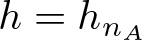 $h = h_{n_A}$. If
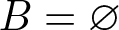 $B = \varnothing$ or
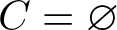 $C = \varnothing$, then we have
 $ \| h \|_{n_{B} \to n_{C}} = \| h \|_{n_A}$.
We now state the random tensor estimate for multiple stochastic integrals from [Reference Chapouto, Li and Oh5, Reference Chapouto, Li, Oh and Zheng7, Reference Oh, Wang and Zine30]. The random tensor estimate was first introduced in a breakthrough work [Reference Deng, Nahmod and Yue12] by Deng, Nahmod, and Yue in the context of random variables; see also [Reference Bringmann2, Reference Oh and Wang29]. See also [Reference Bourgain1] for a precursor of the random tensor estimate. In [Reference Oh, Wang and Zine30], the third author with Wang and Zine extended it to treat the case of iterated Wiener–Ito integrals (namely, with the Hurst parameter 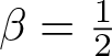 $\beta = \frac 12$), which was further extended in [Reference Chapouto, Li and Oh5, Reference Chapouto, Li, Oh and Zheng7] to the case of multiple stochastic integrals with respect to fractional Brownian motions of Hurst parameter
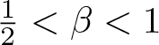 $\frac12 \lt \beta \lt 1$. In the following, we state a slightly simplified version of the random tensor estimate from [Reference Chapouto, Li and Oh5], which is sufficient for our purpose. See [Reference Chapouto, Li and Oh5] for a more general statement and its proof (which follows closely the presentation in [Reference Oh, Wang and Zine30], corresponding to the
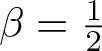 $\beta = \frac 12$ case).
Lemma 3.5. Fix 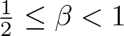 $\frac 12 \le \beta \lt 1$ and let
 $A$ be a finite index set with
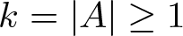 $k = |A| \ge 1$. Given a tensor
 $h=h_{bc n_A} \in \ell^2_{bcn_A}$ with
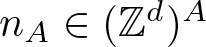 $n_A \in (\mathbb{Z}^d)^{A}$ and
 $(b,c) \in (\mathbb{Z}^d)^{m}$ for some integer
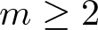 $m\ge2$, satisfying
 \begin{align*}
h_{-b, -c, -n_A} = \overline{h_{bc n_A}},
\quad
(b,c) \in (\mathbb{Z}^d)^{m}, \
n_A \in (\mathbb{Z}^d)^{A},
\end{align*}
define the random tensor 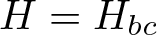 $H = H_{bc}$ by
 \begin{align*}
H_{bc} = \sum_{n_A} I_k \big[ h_{bcn_A} f_{bc} (t_A, n_A) \big]
\end{align*}
for  $f\in \ell^\infty_{bc n_A}( (\mathbb{Z}^d)^{k+m} ; \mathscr{H}^\beta(\mathbb{R}_+^{k}) )$, satisfying
 \begin{align*}
f_{-b, -c, -n_A} = \overline{f_{bc n_A}},
\quad
(b,c) \in (\mathbb{Z}^d)^{m}, \
n_A \in (\mathbb{Z}^d)^{A},
\end{align*}
where 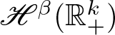 $\mathscr{H}^\beta(\mathbb{R}_+^{k})$ is as in (3.3) and (3.4) (see also (3.2)) and
 $I_k$ denotes the multiple stochastic integral defined in § 3.1. Then, given any
 $\theta \gt 0$ and finite
 $p \ge1$, we have
 \begin{align*}
\big\| \| H_{bc} \|_{b \to c} \big\|_{L^p(\Omega)}
&
\lesssim p^\frac k2
\|f_{bc}(t_A,n_A)\|_{\ell^\infty_{bc n_A}\mathscr{H}^\beta_{t_A}}
\| h_{bcn_A} \|_{\ell^2_{bcn_A}}^{\theta}\\
&
\quad \times \Big( \max_{(B,C)} \| h_{bcn_A} \|_{b n_B \to c n_C} \Big)^{1 - \theta} ,
\end{align*}
where the maximum is taken over all partitions 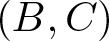 $(B,C)$ of
 $A$.
We note that the Wiener chaos estimate (Lemma 3.2) plays a crucial role in the proof of Lemma 3.5.
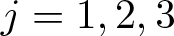
Remark 3.6. In the proofs of Propositions 4.2, 5.2, and 5.3 to study regularity properties of the drivers  $\mathbf{X}^j$,
 $j = 1, 2, 3$, we apply the random tensor estimate (Lemma 3.5). In estimating the
 $\mathscr{H}_{t_A}^\beta$-norm, we first apply (multi-parameter) Sobolev’s inequality and bound it by the
 $L^\frac1\beta$-norm; see (4.25), (5.40), and (5.59). In the current parabolic setting, this suffices for our purpose since there is no oscillatory cancellation to exploit. In the dispersive setting [Reference Chapouto, Gubinelli, Li, Li and Oh4–Reference Chapouto, Li, Oh and Zheng7, Reference Oh and Shao27], however, such an approach based on Sobolev’s inequality would be too crude and we need to estimate the
 $\mathscr{H}_{t_A}^\beta$-norm directly by exploiting subtle oscillatory cancellations.
4. Young case
In this section, we consider the Young case (= the fractional-in-time case with the Hurst parameter 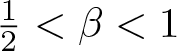 $\frac 12 \lt \beta \lt 1$). As mentioned in §1, our main task is to give a pathwise meaning to the stochastic convolution
 $\Psi(u)$ as the convolution Young integral
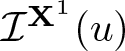 $\mathcal{I}^{\mathbf{X}^1}(u)$ with the first-order driver
 $\mathbf{X}^1$ in (1.11), which allows us to rewrite the Duhamel formulation (1.3) as the following convolution YDE:
 \begin{equation}
u(t) = S(t) u_0 + \mathcal{I}^{\mathbf{X}^1}(u)(t).
\end{equation}
In §4.1, we briefly go over the construction of a convolution Young integral for readers’ convenience. In §4.2, we then use the random tensor estimate (Lemma 3.5) to study regularity properties of the first-order driver  $\mathbf{X}^1$ in (1.11) (including the case
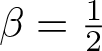 $\beta = \frac12$). In §4.3, by making a suitable choice of parameters, we prove global well-posedness of the convolution YDE (4.1), thus establishing Theorem 1.1.
4.1. Convolution Young integral
In this subsection, we recall the computation from [Reference Gubinelli and Tindel19, Section 4] for readers’ convenience. We first define the auxiliary operator  $\mathbf{Y}$ by
 \begin{equation}
\mathbf{Y}_{t, r}(f)
= \int_r^t
S_{t- t'} [ f
\phi dW^\beta_{t'} ]
\end{equation}
for 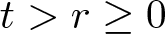 $t \gt r \ge 0$, where
 $f$ is a function on
 $\mathbb{T}$. Then, from (1.4) and (4.2) with (2.5), we formally have
 \begin{equation}
\big(\widehat {\delta} \Psi(u)\big)_{t, r} = \mathbf{Y}_{t, r} (u_\bullet),
\end{equation}
where  $\bullet$ denotes the variable of integration. By replacing
 $\bullet$ in (4.3) by the left endpoint
 $r$, we formally have
 \begin{equation}
\mathbf{Y}_{t, r} (u_\bullet)
= \mathbf{X}^1_{t, r} (u_r)
+ Q_{t, r},
\end{equation}
where  $\mathbf{X}^1$ is the first-order driver defined in (1.11). Here,
 $Q$ is formally given as
 $Q_{t, r} =
\mathbf{Y}_{t, r} ((\widehat {\delta} u)_{\bullet, r})$ but this expression does not play any role in the following.
Our goal is to find one error term  $Q$ with sufficient regularity, which will allow us to define the convolution Young integral
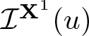 $\mathcal{I}^{\mathbf{X}^1}(u)$ in the pathwise manner as the unique limit of Riemann–Stieltjes type sums; see (4.11) below.
We recall the convolution sewing lemma [Reference Gubinelli and Tindel19, Theorem 3.5], which will be the main tool for constructing the convolution Young integral 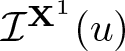 $\mathcal{I}^{\mathbf{X}^1}(u)$ (and also the convolution rough integral
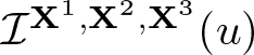 $\mathcal{I}^{\mathbf{X}^1, \mathbf{X}^2, \mathbf{X}^3}(u)$ in §5). See also [Reference Gerasimovičs and Hairer14, Theorem 2.4] and [Reference Friz and Hairer13, Exercise 4.16].
Lemma 4.1. (convolution sewing lemma)
Let  $\gamma \gt 1$,
 $s \in \mathbb{R}$, and
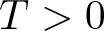 $T \gt 0$.
(i) There exists a unique linear map (called the convolution sewing map)
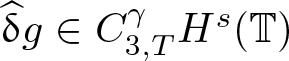
$\widehat \Lambda: C^{\gamma}_{3,T} H^s(\mathbb{T}) \cap
\operatorname{Ker} \widehat {\delta}|_{C_{3,T}H^s_x}
\to C^{\gamma}_{2,T}H^s(\mathbb{T})$ such that
for each\begin{align*}
\widehat {\delta} \widehat \Lambda h = h
\end{align*}
$h\in C_{3,T}H^s(\mathbb{T}^d)\cap \operatorname{Ker} \widehat {\delta}|_{C_{3,T} H^s_x}$, satisfying
for any\begin{align*}
\|\widehat \Lambda h\|_{C^{\gamma-\theta}_{2, T}H^{s+2\theta}_x}
\lesssim \| h\|_{C^\gamma_{3, T} H^s_x}
\end{align*}
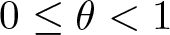
$0 \le \theta \lt 1$ with $\theta \le \gamma$.(ii) Given any
$g\in C_{2,T}H^s(\mathbb{T})$ with $\widehat {\delta} g\in C^\gamma _{3,T}H^s(\mathbb{T})$, there exists unique $f\in C([0, T];H^s(\mathbb{T}))$ (modulo an additive constant) such that $\widehat {\delta} f = (\operatorname{Id} - \widehat \Lambda \widehat {\delta})g$. In addition, we have
for any\begin{align*}
(\widehat {\delta} f)_{t,r} = \lim_{|\Pi([r,t])|\to 0}
\sum_{j=0}^{n-1} S_{t- t_j} g_{t_j,t_{j+1}}
\end{align*}
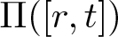
$(t,r)\in \Delta_{2,T}$, where the limit is over any partition $\Pi([r,t])$ of $[r,t]$:
whose mesh size\begin{equation*}\Pi ([r,t]) = \{r = t_{n} \lt \dots \lt t_1 \lt t_0 = t\}\end{equation*}
$|\Pi([r,t])| = \max_{j} |t_j-t_{j+1}|$ tends to $0$.














Let  $\mathbf{X}^1$ be as in (1.11). Then, we have
 \begin{equation}
\widetilde {\delta} \mathbf{X}^1 = 0,
\end{equation}
where  $\widetilde {\delta}$ is as in (2.6). Suppose that we have
 \begin{equation}
\mathbf{X}^1 (\omega)
\in C_{2, T}^{\gamma} \mathcal{L}(H^s(\mathbb{T}))
\end{equation}
for some  $s \in \mathbb{R}$,
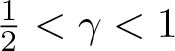 $\frac 12 \lt \gamma \lt 1$, and
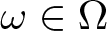 $\omega \in \Omega$. In the following discussion, we suppress the
 $\omega$-dependence. In addition, we assume that
 \begin{equation}
u \in \widehat{\mathcal{C}}_{T}^\alpha H^s(\mathbb{T})
\end{equation}
for some 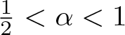 $\frac 12 \lt \alpha \lt 1$, where
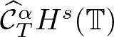 $\widehat{\mathcal{C}}_{T}^\alpha H^s(\mathbb{T})$ is as in (2.11).
By applying the convolution coboundary operator  $\widehat {\delta}$ in (2.5) to (4.4) and noting that, in view of (4.3), the left-hand side of (4.4) formally vanishes under the application of
 $\widehat {\delta}$, any error term
 $Q$ (if it exists) satisfies
 \begin{align*}
\widehat {\delta} Q
= - \widehat {\delta} \big(\mathbf{X}^1 (u) \big)
= \mathbf{X}^1 (\widehat {\delta} u )
\in C_{3, T}^{\alpha + \gamma}H^s(\mathbb{T}),
\end{align*}
where the second equality follows from (2.8) and (4.5). By the assumptions (4.6) and (4.7), we have 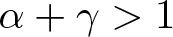 $\alpha + \gamma \gt 1$. Thus, we can apply the convolution sewing lemma (Lemma 4.1) to define an error term
 $Q$ by the relation:
 \begin{equation}
Q = - \widehat \Lambda \widehat {\delta}
\big(\mathbf{X}^1 (u) \big)
\in C_{2, T}^{\alpha + \gamma}H^s(\mathbb{T}),
\end{equation}
where  $\widehat \Lambda$ denotes the convolution sewing map. Therefore, from (4.3), (4.4), and (4.8), we make sense of the stochastic convolution
 $\Psi(u)$ as the convolution Young integral
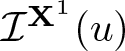 $\mathcal{I}^{\mathbf{X}^1}(u)$ of
 $u$ (with respect to the Young driver
 $\mathbf{X}^1$ in (4.6)):
 \begin{equation}
\Psi(u) = \mathcal{I}^{\mathbf{X}^1}(u)
\end{equation}
where  $\mathcal{I}^{\mathbf{X}^1}(u)(0) = 0$ and its convolution increment is given by
 \begin{equation}
\widehat {\delta} \mathcal{I}^{\mathbf{X}^1}(u)
=
(\operatorname{Id} - \widehat \Lambda \widehat {\delta})\big(\mathbf{X}^1 (u) \big).
\end{equation}
In view of (4.8) with 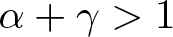 $\alpha + \gamma \gt 1$, the convolution rough integral
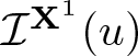 $\mathcal{I}^{\mathbf{X}^1}(u)$ is given by the unique limit of Riemann–Stieltjes type sums:
 \begin{equation}
\mathcal{I}^{\mathbf{X}^1}(u)(t)
= \lim_{|\Pi([0,t])|\to 0}
\sum_{j=0}^{n-1} S_{t- t_j}
\mathbf{X}^1_{t_j,t_{j+1}} (u_{t_{j+1}}),
\end{equation}
where the limit is understood in the sense of Lemma 4.1 (ii). Here, we used the fact that
 \begin{equation}
\lim_{|\Pi([0,t])|\to 0}
\bigg\|\sum_{j=0}^{n-1} S_{t- t_j}
Q_{t_j,t_{j+1}}\bigg\|_{H^s_x}
\le
\lim_{|\Pi([0,t])|\to 0}
\sum_{j=0}^{n-1}
\|Q_{t_j,t_{j+1}}\|_{H^s_x}
= 0,
\end{equation}
provided that 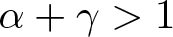 $\alpha + \gamma \gt 1$.
In view of (4.9), the Duhamel formulation (1.3) reduces to the convolution YDE (4.1). The main task that remains is to verify that (4.6) holds for the first-order driver  $\mathbf{X}^1$ defined in (1.11), almost surely, under suitable assumptions on the relevant parameters.
4.2. First-order driver
In this subsection, we study regularity properties of the first-order driver  $\mathbf{X}^1$ in (1.11). From (1.5) and (1.8), we have
 \begin{equation}
\mathbf{X}^1_{t, r}(f)
= \sum_{n\in \mathbb{Z}} e_n
\int_r^t \sum_{n_1, n_2 \in \mathbb{Z}} \mathbf 1_{n = n_{12}}
\cdot e^{-(t-t')\langle n \rangle^2}e^{-(t'-r)\langle n_2 \rangle^2} \widehat f(n_2) \phi_{n_1} d B_{n_1}(t')
\end{equation}
for 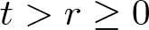 $t \gt r \ge 0$, where
 $n_{12} = n_1 + n_2$ as in (2.1). A direct computation shows that
 $\mathbf{X}^1$ satisfies (4.5).
Proposition 4.2. Let 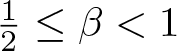 $\frac 12 \le \beta \lt 1$ and
 $s, s_0, \sigma \in \mathbb{R}$. Given
 $\phi \in \operatorname{HS}(L^2(\mathbb{T}); H^\sigma(\mathbb{T}))$ satisfying (1.8), let
 $\mathbf{X}^1$ be the first-order driver in (4.13). Suppose that
 \begin{align}
s + \sigma & \gt - 2a \beta,\cr
s_0 & \lt \min \Big( s\wedge 0 + \sigma + 2a\beta,
\, s + \sigma\wedge 0 + 2a \beta \Big)\cr
\end{align}
for some  $0 \le a \lt 1$. Then, given any finite
 $p \ge 1$, we have
 \begin{equation}
\big\| \| \mathbf{X}^1_{t,r} \|_{\mathcal{L}(H^s; H^{s_0})} \big\|_{L^p(\Omega)}
\lesssim p^\frac 12
\| \phi\|_{\operatorname{HS}(L^2;H^\sigma)}
|t-r|^{(1-a)\beta}
\end{equation}
for any 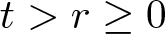 $t \gt r\ge 0$. Consequently, given
 $0 \lt \gamma \lt (1-a)\beta$, we have
 \begin{equation}
\big\| \| \mathbf{X}^1\|_{C^{\gamma}_{2,T} \mathcal{L}(H^s;H^{s_0})} \big\|_{L^p(\Omega)} \lesssim_T
p^\frac 12
\| \phi\|_{\operatorname{HS}(L^2;H^\sigma)}
\end{equation}
for any finite  $p \ge1$ and
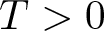 $T \gt 0$. In particular, there exists a version of
 $\mathbf{X}^1$ such that
 \begin{equation*}\mathbf{X}^1 \in C^{\gamma}_{2,T} \mathcal{L}(H^s(\mathbb{T});H^{s_0}(\mathbb{T})), \end{equation*}
almost surely.
Proof. We first note that the bound (4.16) follows from (4.15) and the Garsia–Rodemich–Rumsey inequality (see, for example, [Reference Gubinelli, Koch, Oh and Tolomeo17, Lemma 2.2]) by arguing as in the proof of [Reference Gubinelli, Koch, Oh and Tolomeo17, Lemma 2.3]. Hence, we focus on proving (4.15) in the following.
Fix 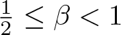 $\frac 12 \le \beta \lt 1$ and
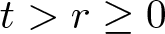 $t \gt r \ge 0$. From (4.13) with (3.6), we have
 \begin{equation}
{\mathcal{F}}_x\big(\langle \nabla \rangle^{s_0}\mathbf{X}^1_{t,r} \langle \nabla \rangle^{-s}f \big)(n)
= \sum_{n_2\in \mathbb{Z}} \widehat f (n_2) I_1[ \mathfrak{h}^1_{nn_2}(n_1) \mathfrak{g}^1_{nn_2}(t') ] ,
\end{equation}
where 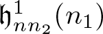 $\mathfrak{h}^1_{nn_2}(n_1) $ and
 $\mathfrak{g}^1_{nn_2}$ are defined by
 \begin{align}
\mathfrak{h}^1_{n n_2}(n_1) & =
\mathbf 1_{n=n_{12}}
\cdot
\frac{\langle n \rangle^{s_0}}{\langle n_2 \rangle^{s}} \phi_{n_1} , \cr
\mathfrak{g}^1_{nn_2} (t') &=
\mathfrak{g}_{nn_2}^{1, t, r} (t')=
\mathbf 1_{[r, t]}(t')\cdot
e^{-(t-t') \langle n \rangle^2}e^{-(t' -r) \langle n_2 \rangle^2}.\cr
\end{align}
Given a dyadic triple  $\textbf{N}_2= (N, N_1, N_2) \in (2^{\mathbb{Z}_{\ge 0}})^3$, we set
 \begin{align}
\mathfrak{h}^{1, \textbf{N}_2}_{n n_2}(n_1) & =
\mathfrak{h}^{1, N, N_1, N_2}_{n n_2}(n_1)
= \mathbf 1_{E_{\textbf{N}_2}}
\cdot
\mathfrak{h}^1_{n n_2}(n_1), \cr
\mathfrak{g}^{1, \textbf{N}_2}_{nn_2} (t') &=
\mathfrak{g}^{1, N, N_1, N_2}_{nn_2} (t') =
\mathbf 1_{E_{\textbf{N}_2}}
\cdot
\mathfrak{g}^1_{nn_2} (t'), \cr
\end{align}
where  $E_{\textbf{N}_2}$ is defined by
 \begin{align*}
E_{\textbf{N}_2} = \big\{(n, n_1, n_2) \in \mathbb{Z}^3:
\ & n = n_1 + n_2, \cr
&
|n|\sim N, \, |n_j|\sim N_j, \, j = 1, 2\big\}.
\end{align*}
On  $E_{\textbf{N}_2}$, we have
 \begin{equation}
\max(N, N_1, N_2) \sim \operatorname{med} (N, N_1, N_2),
\end{equation}
where the right-hand side denotes the second largest among  $N$,
 $N_1$, and
 $N_2$. We define
 $\mathcal{D}_2$ by setting
 \begin{equation}
\mathcal{D}_2 = \left\{
\textbf{N}_2 = (N, N_1, N_2)\in (2^{\mathbb{Z}_{\ge 0}})^3: \, \textbf{N}_2\ \text{satisfies (4.20)}
\right\}.
\end{equation}
Given any  $\theta \gt 0$, it follows from (4.17), (4.18), (4.19), and the random tensor estimate (Lemma 3.5) with (1.9) that
 \begin{align}
\big\| & \| \mathbf{X}^1_{t,r} \|_{\mathcal{L}(H^s;H^{s_0})} \big\|_{L^p(\Omega)}
= \big\| \| \langle \nabla \rangle^{s_0}\mathbf{X}^1_{t,r}\langle \nabla \rangle^{-s} \|_{\mathcal{L}(L^2;L^2)} \big\|_{L^p(\Omega)}\cr
& = \big\| \| I_1[ \mathfrak{h}^1_{nn_2}(n_1) \mathfrak{g}^1_{nn_2}(t') ] \|_{\ell^2_{n_2} \to \ell^2_n} \big\|_{L^p(\Omega)}\cr
& \le \sum_{\textbf{N}_2 \in \mathcal{D}_2}
\big\| \|
I_1[ \mathfrak{h}^{1, \textbf{N}_2}_{nn_2}(n_1) \mathfrak{g}^{1, \textbf{N}_2}_{nn_2}(t')] \|_{\ell^2_{n_2} \to \ell^2_n} \big\|_{L^p(\Omega)}\cr
& \lesssim
p^\frac 12
\sum_{\textbf{N}_2\in \mathcal{D}_2}
\frac{N_{\max}^{\frac 12 \theta} N^{\theta s_0}}
{N_1^{\theta\sigma} N_2^{\theta s}}
\|\phi\|_{\operatorname{HS}(L^2; H^\sigma)}^\theta
\| \mathfrak{g}^{1, \textbf{N}_2}_{nn_2} (t')\|_{\ell^\infty_{nn_2} \mathscr{H}_{t'}^\beta}\cr
& \quad\times
\max\Big( \| \mathfrak{h}^{1, \textbf{N}_2}_{nn_2}(n_1)\|_{n_1n_2 \to n} ,
\| \mathfrak{h}^{{I}, \textbf{N}_2}_{nn_2}(n_1) \|_{n_2 \to n n_1} \Big)^{1-\theta}\cr
\end{align}
for any finite  $p \ge 1$, where
 $N_{\max} = \max(N, N_1, N_2)$ and
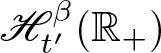 $\mathscr{H}^\beta_{t'}(\mathbb{R}_+)$ is as in (3.2).
From (4.19), (4.18), and Cauchy–Schwarz’s inequality with (1.9), we have
 \begin{align}
\| \mathfrak{h}^{1, \textbf{N}_2}_{nn_2}(n_1)\|_{n_1n_2 \to n}
&\sim
\frac{N^{s_0}}{N_2^s}
\sup_{\|f\|_{\ell^2_{n_1 n_2}}
= \|g\|_{\ell^2_{n}} = 1}
\bigg|
\sum_{n, n_1, n_2 \in \mathbb{Z}}
\mathbf 1_{E_{\textbf{N}_2}}
\cdot
\phi_{n_1} f_{n_1n_2} g_{n}\bigg|\cr
&\lesssim
\frac{N^{s_0}}{N_1^\sigma N_2^s}
\|\phi\|_{\operatorname{HS}(L^2; H^\sigma)}.
\end{align}
A similar computation yields
 \begin{equation}
\| \mathfrak{h}^{1, \textbf{N}_2}_{nn_2}(n_1)\|_{n_2 \to n n_1} \lesssim \frac{N^{s_0}}{N_1^\sigma N_2^s} \|\phi\|_{\operatorname{HS}(L^2; H^\sigma)}.
\end{equation}
Next, we estimate the  $\mathscr{H}^\beta_{t'}$-norm of
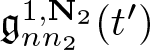 $ \mathfrak{g}_{nn_2}^{1, \textbf{N}_2}(t')$ appearing in (4.22). From (3.2) and Sobolev’s inequality, we have
 \begin{equation}
\| \mathfrak{g}^1_{nn_2} (t')\|_{\ell^\infty_{nn_2} \mathscr{H}_{t'}^\beta}
=
\| \mathfrak{g}^1_{nn_2} (t')\|_{\ell^\infty_{nn_2} \dot H_{t'}^{\frac 12 - \beta}}
\lesssim
\| \mathfrak{g}^1_{nn_2} (t')\|_{\ell^\infty_{nn_2} L^\frac 1\beta_{t'} }.
\end{equation}
Before proceeding further, recall the beta function 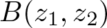 $B(z_1, z_2)$ defined by
 \begin{equation}
B(z_1, z_2) = \int_0^1 (1-t)^{z_1 - 1} t^{z_2-1} dt,
\end{equation}
which is finite for  ${\text{Re}}\, z_1, {\text{Re}}\, z_2 \gt 0$. Then, it follows from (4.18), the boundedness of
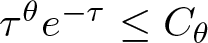 $\tau^\theta e^{- \tau} \le C_\theta$ for any
 $\tau \ge 0$ (given
 $\theta \ge 0$), and a change of variables with (4.26) that
 \begin{align}
\| \mathfrak{g}^1_{nn_2} (t')\|_{L^\frac 1\beta_{t'} }^\frac 1 \beta
& = J^1_{t, r}(n, n_2)\cr
: \! & = \int_r^t
e^{-\beta^{-1}(t-t') \langle n \rangle^2}e^{-\beta^{-1}(t' -r) \langle n_2 \rangle^2}
dt' \cr
& \lesssim_{\beta, a_1, a_2}
\langle n \rangle^{-2a_1}\langle n_2 \rangle^{-2a_2}
\int_r^t (t - t')^{-a_1}
(t' - r)^{-a_2} dt'\cr
& = (t-r)^{1-a_1 - a_2}\langle n \rangle^{-2a_1}\langle n_2 \rangle^{-2a_2}
B(1- a_1 , 1- a_2)\cr
& \sim_{a_1, a_2} (t-r)^{1-a_1 - a_2}\langle n \rangle^{-2a_1}\langle n_2 \rangle^{-2a_2}, \cr
\end{align}
uniformly in 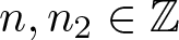 $n, n_2 \in \mathbb{Z}$ and
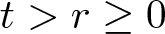 $t \gt r\ge 0$, provided that
 $0 \le a_1, a_2 \lt 1$. Hence, we have
 \begin{equation}
\| \mathfrak{g}^{1, \textbf{N}_2}_{nn_2} (t')\|_{L^\frac 1\beta_{t'} } \lesssim (t-r)^{(1-a)\beta}N_{\max}^{-2a\beta},
\end{equation}
uniformly in 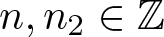 $n, n_2 \in \mathbb{Z}$, dyadic
 $N, N_1, N_2 \ge 1$, and
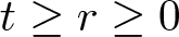 $t \ge r\ge 0$, provided that
 $0 \le a \lt 1$.
Therefore, putting (4.22), (4.23), (4.24), (4.25), and (4.28) together with (4.21), we obtain
 \begin{align}
\big\| \| & \mathbf{X}^1_{t,r} \|_{\mathcal{L}(H^s;H^{s_0})} \big\|_{L^p(\Omega)}\cr
& \lesssim
p^\frac 12
\|\phi\|_{\operatorname{HS}(L^2; H^\sigma)}
|t- r|^{(1-a) \beta}
\sum_{\textbf{N}_2\in \mathcal{D}_2}
N_{\max}^{\frac 12 \theta - 2a\beta }
\frac{N^{s_0}}{N_1^{\sigma} N_2^{s}}\cr
& \lesssim
p^\frac 12
\|\phi\|_{\operatorname{HS}(L^2; H^\sigma)}
|t- r|^{(1- a) \beta}
\end{align}
for any  $0 \le a \lt 1$, provided that (4.14) holds and that
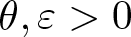 $\theta, \varepsilon \gt 0$ are sufficiently small. Here, the second inequality in (4.29) follows from separately considering the cases: (a)
 $N \sim N_1 \gt rsim N_2$, (b)
 $N \sim N_2 \gg N_1$, and (c)
 $N_1 \sim N_2 \gg N$ (also depending on the sign of the exponent of
 $N_{\min}$).
4.3. Proof of Theorem 1.1
We conclude this section by presenting a proof of Theorem 1.1. More precisely, we prove that the convolution YDE (4.1) is pathwise globally well-posed. We note that, once we make a suitable choice of parameters, the rest follows from a standard pathwise well-posedness argument for a YDE. See, for example, [Reference Chouk, Gubinelli, Li, Li and Oh9, Subsection 3.3].
Proof of Theorem 1.1
Given 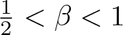 $\frac 12 \lt \beta \lt 1$, let
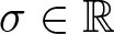 $\sigma \in \mathbb{R}$ satisfy (1.10). Let
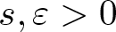 $s, \varepsilon \gt 0$ sufficiently small such that
 \begin{equation}
\sigma - s \gt - 2 \beta + 1 + 6\varepsilon.
\end{equation}
By taking  $\varepsilon \gt 0$ possibly smaller such that
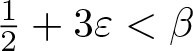 $\frac 12 + 3\varepsilon \lt \beta$, set
 $a = 1 - \frac1 {2\beta} - \frac {3\varepsilon} \beta \in (0, 1)$ such that
 \begin{equation}
(1-a) \beta = \frac 12 + 3\varepsilon.
\end{equation}
Then, the conditions in (4.14) with  $s_0 = s \gt 0$ and
 $\sigma \lt 0$ reduce to (4.30), which is satisfied by our choice of parameters. Hence, it follows from Proposition 4.2 with
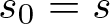 $s_0 = s$ that there exists
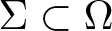 $\Sigma \subset \Omega$ with
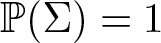 $\mathbb{P}(\Sigma) = 1$ such that, for each
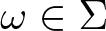 $\omega \in \Sigma$, we have
 \begin{align*}
\mathbf{X}^1
= \mathbf{X}^1 (\omega)
\in \bigcap_{j = 1}^\infty C^{\frac 12 +2\varepsilon}_{2,j} \mathcal{L}(H^s(\mathbb{T})).
\end{align*}
In the following, we fix 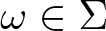 $\omega \in \Sigma$ and often suppress dependence on
 $\omega$.
Fix  $0 \lt T \le 1$ (to be chosen later). Define a map
 ${\Gamma}$ on
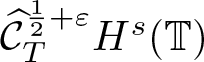 $\widehat{\mathcal{C}}_{T}^{\frac 12 + \varepsilon} H^s(\mathbb{T})$ by setting
 \begin{align}
{\Gamma}(u)(t)
& = S(t) u_0 + \mathcal{I}^{\mathbf{X}^1}(u)(t)\cr
& = S(t) u_0 +
\big[(\operatorname{Id} - \widehat \Lambda \widehat {\delta})(\mathbf{X}^1(u))\big]_{t, 0}.
\end{align}
See (4.10). From (2.9) with (2.7), we have
 \begin{align}
\| \mathbf{X}^1(u) \|_{C_{2, T}^{\frac 12 +\varepsilon} H^s_x}
& \le T^\varepsilon \| \mathbf{X}^1(u) \|_{C_{2, T}^{\frac 12 +2\varepsilon} H^s_x}
\le T^\varepsilon \|\mathbf{X}^1\|_{C^{\frac 12 +2\varepsilon}_{2, 1} \mathcal{L}(H^s)}
\| u \|_{L^\infty_T H^s_x}\cr
& \lesssim T^\varepsilon \|\mathbf{X}^1\|_{C^{\frac 12 +2\varepsilon}_{2, 1} \mathcal{L}(H^s)}
\| u \|_{\widehat{\mathcal{C}}_{T}^{\frac 12 +\varepsilon} H^s_x}.
\end{align}
By applying the convolution sewing lemma (Lemma 4.1) with (2.9), we have
 \begin{align}
\|\widehat \Lambda \mathbf{X}^1(\widehat {\delta} u)\|_{C_{2, T}^{\frac 12 + \varepsilon} H^s_x}
& \le T^{\frac 12 + 2\varepsilon }
\|\widehat \Lambda \mathbf{X}^1(\widehat {\delta} u)\|_{C_{2, T}^{1+3\varepsilon} H^{s}_x}\cr
& \lesssim
T^{\frac 12 + 2\varepsilon }
\|\mathbf{X}^1(\widehat {\delta} u)\|_{C_{3, T}^{1+ 3\varepsilon} H^{s}_x}\cr
& \lesssim
T^{\frac 12 + 2\varepsilon }
\|\mathbf{X}^1\|_{C_{2, 1}^{\frac 12 + 2\varepsilon} \mathcal{L}(H^s)}
\| u \|_{\widehat{\mathcal{C}}_{T}^{\frac 12 + \varepsilon} H^s_x}.
\end{align}
From (4.32), (4.33), and (4.34) with (2.11), we have
 \begin{equation}
\| {\Gamma}(u) \|_{\widehat{\mathcal{C}}_{T}^{\frac 12 +\varepsilon} H^s_x} \lesssim \|u_0 \|_{H^s}+ T^\varepsilon \|\mathbf{X}^1\|_{C^{\frac 12 +2\varepsilon}_{2, 1} \mathcal{L}(H^s)}
\| u \|_{\widehat{\mathcal{C}}_{T}^{\frac 12 +\varepsilon} H^s_x}.
\end{equation}
A similar computation yields the following difference estimate:
 \begin{equation}
\| {\Gamma}(u) - {\Gamma}(v) \|_{\widehat{\mathcal{C}}_{T}^{\frac 12 +\varepsilon} H^s_x} \lesssim T^\varepsilon \|\mathbf{X}^1\|_{C^{\frac 12 +2\varepsilon}_{2, 1} \mathcal{L}(H^s)}
\| u -v\|_{\widehat{\mathcal{C}}_{T}^{\frac 12 +\varepsilon} H^s_x}.
\end{equation}
Hence, by choosing
 \begin{equation}
T = T\big( \|\mathbf{X}^1(\omega) \|_{C^{\frac 12 +2\varepsilon}_{2, 1} \mathcal{L}(H^s)}\big) \gt 0
\end{equation}
sufficiently small, it follows from (4.35) and (4.36) that  ${\Gamma}$ is a contraction on
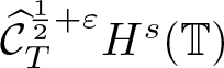 $ \widehat{\mathcal{C}}_{T}^{\frac 12 + \varepsilon} H^s(\mathbb{T})$. Therefore, by the Banach fixed point theorem, there exists a unique fixed point
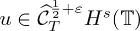 $u \in \widehat{\mathcal{C}}_{T}^{\frac 12 + \varepsilon} H^s(\mathbb{T})$ such that
 \begin{align*}
u (t)= {\Gamma}(u)(t) = S(t) u_0 + \mathcal{I}^{\mathbf{X}^1}(u)(t).
\end{align*}
Namely,  $u$ is a unique solution to the convolution YDE (4.1).
Thanks to the linearity of 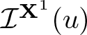 $\mathcal{I}^{\mathbf{X}^1}(u)$ in
 $u$, the local existence time
 $T$ in (4.37) is independent of the initial data
 $u_0$. Given a target time
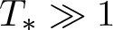 $T_* \gg1$, we now choose a (smaller) local existence time
 \begin{align*}
T = T\big( \|\mathbf{X}^1(\omega) \|_{C^{\frac 12 +2\varepsilon}_{2, T_*} \mathcal{L}(H^s)}\big) \gt 0
\qquad \text{such that}\qquad
T^\varepsilon \|\mathbf{X}^1\|_{C^{\frac 12 +2\varepsilon}_{2, T_*} \mathcal{L}(H^s)} \ll 1.
\end{align*}
Then, by iteratively applying the contraction argument on each time interval  $[jT, (j+1)T]\cap [0, T_*]$,
 $j = 0,1, \dots, \big[\frac {T_*}T\big] $, where
 $[x]$ denotes the integer part of
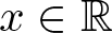 $x \in \mathbb{R}$, we can extend the solution
 $u$ to (4.1) onto the entire interval
 $[0, T_*]$. This proves pathwise global well-posedness.
Remark 4.3. In § 5, we treat the rough case (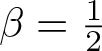 $\beta = \frac 12$) by considering the third-order expansion. We point out that, even in the fractional-in-time case (
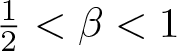 $\frac 12 \lt \beta \lt 1$), we can improve the regularity restrictions (1.10) by working with the third-order expansion, where we only impose the temporal regularity of
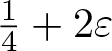 $\frac 14 + 2\varepsilon$ on the relevant drivers. Then, instead of (4.31), we have
 \begin{align*}
(1-a) \beta = \frac 14 + 3\varepsilon,
\end{align*}
which yields  $ \sigma - s \gt - 2 \beta + \frac 12 + 6\varepsilon$, leading to an improvement of
 $\frac12$ for the range of
 $\sigma$ (regarding boundedness of the first-order driver
 $\mathbf{X}^1$). See also Remark 1.5 (ii). We, however, do not pursue this issue, since our purpose here is to compare our approach with that in [Reference Gubinelli and Tindel19, Section 4].
5. Rough case
In this section, we consider the rough case (= the white-in-time case with 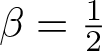 $\beta = \frac 12$). In this case, the first-order driver
 $\mathbf{X}^1$ in (1.11) is not sufficient and thus we need to augment it by introducing higher-order drivers
 $\mathbf{X}^j$,
 $j \ge 2$, via the relation:
 \begin{equation}
\mathbf{X}^j_{t, r} = \mathbf{Y}_{t, r} \circ \mathbf{X}^{j-1}_{\bullet, r},
\end{equation}
where  $\mathbf{Y}$ is as in (4.2) and
 $\bullet$ denotes the variable of integration. Namely, we have
 \begin{equation}
\mathbf{X}^{j}_{t, r}(f) =
\int_r^t S_{t-t'} \big[ \mathbf{X}^{j - 1}_{t', r} (f)\phi dW^\beta_{t'}\big].
\end{equation}
Then, Chen’s relation in the current convolution setting reads as
 \begin{equation}
\widetilde {\delta} \mathbf{X}^n = \sum_{j = 1}^{n-1}\mathbf{X}^j \mathbf{X}^{n - j},
\end{equation}
where  $\widetilde {\delta} $ is as in (2.6); see [Reference Gubinelli and Tindel19, p. 40].
By following [Reference Gubinelli and Tindel19, Section 5], we consider a third-order rough path  $\overline{\mathbf{X}} = (\mathbf{X}^1, \mathbf{X}^2, \mathbf{X}^3)$ and make sense of the stochastic convolution
 $\Psi(u)$ as a convolution rough integral
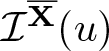 $\mathcal{I}^{\overline{\mathbf{X}}}(u)$. This allows us to rewrite the Duhamel formulation (1.3) as the following convolution RDE:
 \begin{equation}
u(t) = S(t) u_0 + \mathcal{I}^{\overline{\mathbf{X}}}(u)(t).
\end{equation}
In §5.1, we briefly go over the construction of a convolution rough integral for readers’ convenience. In §5.2, we then use the random tensor estimate (Lemma 3.5) to study regularity properties of the second- and third-order drivers  $\mathbf{X}^2$ and
 $\mathbf{X}^3$ (for the range
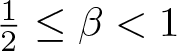 $\frac 12 \le \beta \lt 1$). In § 5.3, we prove global well-posedness of the convolution RDE (5.4), thus establishing Theorem 1.3.
5.1. Convolution rough integral
Following the presentation in [Reference Gubinelli and Tindel19, Section 5], we consider a second-order controlled path in the current convolution setting.
Definition 5.1. Let  $V$ be a separable Banach space and
 $\{S_t\}_{t \in \mathbb{R}_+} \subset \mathcal{L}(V)$ be a semigroup of bounded operators with
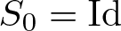 $S_0 = \operatorname{Id}$. Fix
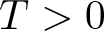 $T \gt 0$.
(i) Given a pair  $(\mathbf{X}^1, \mathbf{X}^2)
\in C_{2, T}^\gamma \mathcal{L}(V)\times C_{2, T}^{2\gamma} \mathcal{L}(V)$ of drivers with
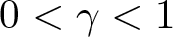 $0 \lt \gamma \lt 1$, we say that
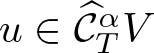 $u \in \widehat{\mathcal{C}}_{T}^\alpha V$ for some
 $0 \lt \alpha \lt 1$ is controlled by
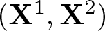 $(\mathbf{X}^1, \mathbf{X}^2)$ if there exist
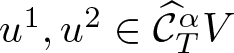 $u^1, u^2 \in \widehat{\mathcal{C}}^\alpha_{T}V$ and remainder terms
 $R^j \in C_{2, T}^{\alpha + (2-j)\gamma} V$,
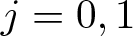 $j = 0, 1$, such that
 \begin{align}
(\widehat {\delta} u)_{t, r} & = \mathbf{X}^1_{t, r} (u^1_r) + \mathbf{X}^2_{t, r}(u^2_r) + R^0_{t, r}, \cr
(\widehat {\delta} u^1)_{t, r} & = \mathbf{X}^1_{t, r} (u^2_r) + R^1_{t, r}
\end{align}
for  $0 \le r \lt t \le T$, where
 $\widehat {\delta}$ is as in (2.5) with the given semigroup
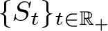 $\{S_t\}_{t \in \mathbb{R}_+}$. We refer to
 $u^j$,
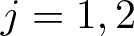 $j = 1, 2$, as the
 $j$th Gubinelli derivative of
 $u$ (with respect to the driver
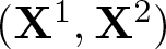 $ (\mathbf{X}^1, \mathbf{X}^2)$). We denote the space of such controlled paths
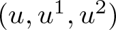 $(u,u^1, u^2)$ by
 $\mathcal{D}_{\mathbf{X}^1, \mathbf{X}^2, T}^{\alpha, \gamma}(V)
= \mathcal{D}_{\mathbf{X}^1, \mathbf{X}^2}^{\alpha, \gamma}([0, T]; V)$ and endow it with the following norm:
 \begin{align}
\| (u, u^1, u^2) \|_{\mathcal{D}^{\alpha, \gamma}_{\mathbf{X}^1, \mathbf{X}^2, T}(V)}
& = \|u(0) \|_{V} + \|u^1\|_{\widehat{\mathcal{C}}_T^\alpha V}+ \|u^2\|_{\widehat{\mathcal{C}}_T^\alpha V}\cr
& \quad
+ \| R^0 \|_{C^{\alpha + 2\gamma}_{2, T}V}
+ \| R^1 \|_{C^{\alpha + \gamma}_{2, T}V},
\end{align}
where  $R^0 $ and
 $R^1$ are defined by the relation (5.5).
(ii) Let 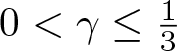 $0 \lt \gamma \le \frac 13$. We say that a triplet
 $(\mathbf{X}^1, \mathbf{X}^2, \mathbf{X}^3)
\in \prod_{j = 1}^3 C_{2, T}^{j\gamma} \mathcal{L}(V)$ is a
 $\gamma$-Hölder convolution rough path if it satisfies the Chen’s relation in the current convolution setting:
 \begin{equation}
\widetilde {\delta} \mathbf{X}^1 = 0, \qquad
\widetilde {\delta} \mathbf{X}^2 = \mathbf{X}^1 \mathbf{X}^1, \qquad
\widetilde {\delta} \mathbf{X}^3 = \mathbf{X}^1 \mathbf{X}^2
+ \mathbf{X}^2 \mathbf{X}^1,
\end{equation}

In our setting, we take 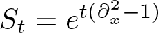 $S_t = e^{t(\partial_x^2- 1)}$ and
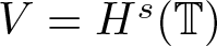 $V = H^s(\mathbb{T})$. As in the Young case discussed in § 4, our goal is to provide a meaning to the stochastic convolution
 $\Psi(u)$ in (1.4) whose convolution increment is formally given by
 \begin{equation}
\big(\widehat {\delta} \Psi(u)\big)_{t, r} = \mathbf{Y}_{t, r} (u_\bullet),
\end{equation}
where  $\mathbf{Y}$ is as in (4.2) and
 $\bullet$ denotes the variable of integration.
For 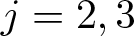 $j = 2, 3$, let
 $\mathbf{X}^j$ be as in (5.1), which satisfies Chen’s relation (5.7). Suppose that
 \begin{equation}
\overline{\mathbf{X}} (\omega)= (\mathbf{X}^1(\omega), \mathbf{X}^2(\omega), \mathbf{X}^3(\omega))
\in \prod_{j = 1}^3 C_{2, T}^{j\gamma} \mathcal{L}(H^s(\mathbb{T}))
\end{equation}
for some  $s \in \mathbb{R}$,
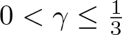 $0 \lt \gamma \le \frac 13$, and
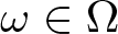 $\omega \in \Omega$. In the following discussion, we suppress the
 $\omega$-dependence. In view of (5.4), we assume that
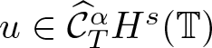 $u
\in \widehat{\mathcal{C}}_{T}^\alpha H^s(\mathbb{T})$ for some
 $0 \lt \alpha \lt 1$ is controlled by
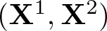 $(\mathbf{X}^1, \mathbf{X}^2)$ with its Gubinelli derivatives
 \begin{equation}
u^1 = u^2 = u\in \widehat{\mathcal{C}}_{T}^\alpha H^s(\mathbb{T}).
\end{equation}
(In fact, (5.10) follows as a result of a contraction argument; see (5.88).) Namely, we have
 \begin{align*}
(\widehat {\delta} u)_{t, r} & = \mathbf{X}^1_{t, r} (u_r) + \mathbf{X}^2_{t, r}(u_r) + R^0_{t, r}, \\
(\widehat {\delta} u)_{t, r} & = \mathbf{X}^1_{t, r} (u_r) + R^1_{t, r},
\end{align*}
where
 \begin{equation}
R^j \in C_{2, T}^{\alpha + (2-j)\gamma} H^s(\mathbb{T}), \quad j = 0, 1.
\end{equation}
In the following, we recall the discussion from [Reference Gubinelli and Tindel19, Section 5] for readers’ convenience. For computational clarity, however, we use  $u^1$ and
 $u^2$ to denote the Gubinelli derivatives of
 $u$. By replacing
 $\bullet$ in (5.8) by the left endpoint
 $r$, we have
 \begin{equation}
\mathbf{Y}_{t, r} (u_\bullet)
= \mathbf{X}^1_{t, r} (u_r)
+ \mathbf{Y}_{t, r} (\widehat {\delta} u_{\bullet, r}).
\end{equation}
See (4.4). Then, by applying (5.5) and (5.1) to (5.12), we have
 \begin{equation}
\mathbf{Y}_{t, r} (u_\bullet)
= \mathbf{X}^1_{t, r} (u_r)
+ \mathbf{X}^2_{t, r} (u_r^1)
+ \mathbf{X}^3_{t, r} (u_r^2)
+ Q_{t, r} ,
\end{equation}
where 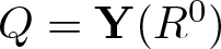 $Q = \mathbf{Y}(R^0)$. As in the Young case, our goal is to find one error term
 $Q$ with sufficient regularity, which will allow us to define the convolution rough integral
 $\mathcal{I}^{\overline{\mathbf{X}}}(u) = \mathcal{I}^{\mathbf{X}^1, \mathbf{X}^2, \mathbf{X}^3}(u)$ in the pathwise manner as the unique limit of Riemann–Stieltjes type sums; see (5.19) below.
By applying the convolution coboundary operator  $\widehat {\delta}$ in (2.5) to (5.13), any error term
 $Q$ (if it exists) satisfies
 \begin{equation}
\widehat {\delta} Q
= - \widehat {\delta} \big[\mathbf{X}^1 (u)
+ \mathbf{X}^2 (u^1)
+ \mathbf{X}^3 (u^2) \big],
\end{equation}
where we used the short-hand notation (2.7). By applying the product rule (2.8) (where 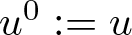 $u^0:= u$) with (5.7) and (5.5), we obtain
 \begin{align}
\widehat {\delta} Q
& = \sum_{j = 1}^3\Big( - (\widetilde {\delta} \mathbf{X}^j) (u^{j-1}) + \mathbf{X}^j (\widehat {\delta} u^{j-1})\Big)\cr
& = \mathbf{X}^1\big(\widehat {\delta} u - \mathbf{X}^1 (u^1) - \mathbf{X}^2 (u^2)\big)
+ \mathbf{X}^2\big(\widehat {\delta} u^1 - \mathbf{X}^1 (u^2)\big)
+ \mathbf{X}^3(\widehat {\delta} u^2)\cr
& = \mathbf{X}^1(R^0) +
\mathbf{X}^2(R^1)
+ \mathbf{X}^3(\widehat {\delta} u^2).
\end{align}
See [Reference Gubinelli and Tindel19, (90)]. From (5.15), (5.9), (5.10), (5.11) with (2.9), we obtain that
 \begin{align*}
\widehat {\delta} Q \in C_{3, T}^{\alpha + 3\gamma}H^s(\mathbb{T}).
\end{align*}
Hence, if  $\alpha + 3\gamma \gt 1$, then we can apply the convolution sewing lemma (Lemma 4.1) to define an error term
 $Q$ by the relation:
 \begin{equation}
Q = - \widehat \Lambda \widehat {\delta}
\big[\mathbf{X}^1 (u)
+ \mathbf{X}^2 (u^1)
+ \mathbf{X}^3 (u^2) \big]
\in C_{2, T}^{\alpha + 3\gamma}H^s(\mathbb{T}),
\end{equation}
where  $\widehat \Lambda$ denotes the convolution sewing map. Therefore, from (5.8), (5.13), and (5.16), we can make sense of the stochastic convolution
 $\Psi(u)$ as the convolution rough integral
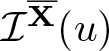 $\mathcal{I}^{\overline{\mathbf{X}}}(u)$ of
 $u$ (with respect to the driver
 $\overline{\mathbf{X}}= (\mathbf{X}^1, \mathbf{X}^2, \mathbf{X}^3)$):
 \begin{equation}
\Psi(u) = \mathcal{I}^{\overline{\mathbf{X}}}(u)
\end{equation}
where 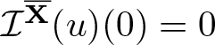 $\mathcal{I}^{\overline{\mathbf{X}}}(u)(0) = 0$ and its convolution increment is given by
 \begin{equation}
\widehat {\delta} \mathcal{I}^{\overline{\mathbf{X}}}(u)
=
(\operatorname{Id} - \widehat \Lambda \widehat {\delta}) \big[\mathbf{X}^1 (u)
+ \mathbf{X}^2 (u^1)
+ \mathbf{X}^3 (u^2) \big].
\end{equation}
In view of (5.16) with  $\alpha + 3\gamma \gt 1$, the convolution rough integral
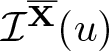 $\mathcal{I}^{\overline{\mathbf{X}}}(u)$ is given by the unique limit of Riemann–Stieltjes type sums:
 \begin{align}
\mathcal{I}^{\overline{\mathbf{X}}}(u)(t)
& = \lim_{|\Pi([0,t])|\to 0}
\sum_{j=0}^{n-1} S_{t- t_j}
\big[\mathbf{X}^1_{t_j,t_{j+1}} (u_{t_{j+1}}) \cr
&
\qquad\qquad\qquad\qquad\quad\,\,\,+ \mathbf{X}^2_{t_j,t_{j+1}} (u^1_{t_{j+1}})
+ \mathbf{X}^3_{t_j,t_{j+1}} (u^2_{t_{j+1}}) \big],
\end{align}
where the limit is understood in the sense of Lemma 4.1 (ii). Here, we used (4.12), which holds for  $\alpha + 3\gamma \gt 1$ in the current setting.
In view of (5.17), the Duhamel formulation (1.3) reduces to the convolution RDE (5.4). As in the Young case, the main task is then to verify that (5.9) holds, almost surely, under suitable assumptions on the relevant parameters.
5.2. Higher-order drivers
In this subsection, we study regularity properties of the second- and third-order drivers  $\mathbf{X}^j$,
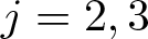 $j = 2, 3$, for
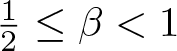 $\frac 12 \le \beta \lt 1$. From (5.1) with (1.11) and (4.2), we formally have
 \begin{equation}
\mathbf{X}^2_{t, r}(f) = \int_r^t
S_{t- t_1} \bigg[\int_r^{t_1} S_{t_1 - t_2}
\big[ (S_{t_2 - r} f)
\phi dW^\beta_{t_2} \big]
\phi dW^\beta_{t_1}\bigg]
\end{equation}
and
 \begin{align}
\mathbf{X}^3_{t, r}(f)
& = \int_r^t
S_{t- t_1} \bigg[\int_r^{t_1} S_{t_1 - t_2}
\Big[\int_r^{t_2} S_{t_2 - t_3} \cr
&
\qquad\qquad\quad\, \big[ (S_{t_3 - r} f)
\phi dW^\beta_{t_3} \big]
\phi dW^\beta_{t_2} \Big]
\phi dW^\beta_{t_1}\bigg]
\end{align}
for 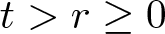 $t \gt r \ge 0$, where
 $f$ is a function on
 $\mathbb{T}$. Here, the iterated stochastic integrals in (5.20) and (5.21) are to be interpreted as multiple Wiener integrals introduced in § 3.1. See (5.34) and (5.54).
In view of (5.20) and (5.21) with (1.5) and (1.8), we can write  $\mathbf{X}^2$ and
 $\mathbf{X}^3$ as
 \begin{align}
\mathbf{X}^2_{t, r}(f)
&
= \sum_{n\in \mathbb{Z}} e_n
\int_r^t
\int_r^{t_1}
\sum_{n_1, n_2, n_3 \in \mathbb{Z}}
\mathbf 1_{n = n_{123}} \cr
&
\quad\times e^{-(t-t_1)\langle n \rangle^2}
e^{-(t_1-t_2)\langle n_{23} \rangle^2}
e^{- (t_2-r)\langle n_3 \rangle^2}
\widehat f(n_3)\cr
&
\quad\times
\prod_{j = 1}^2 \phi_{n_j} dB_{n_j}(t_j)
\end{align}
and
 \begin{align}
\mathbf{X}^3_{t, r}(f)
&
= \sum_{n\in \mathbb{Z}} e_n
\int_r^t
\int_r^{t_1}
\int_r^{t_2}
\sum_{n_1, \dots, n_4 \in \mathbb{Z}}
\mathbf 1_{n = n_{1234}} \cr
&
\quad\times e^{-(t-t_1)\langle n \rangle^2}
e^{-(t_1-t_2)\langle n_{234} \rangle^2}
e^{-(t_2-t_3)\langle n_{34} \rangle^2}
e^{-(t_3-r)\langle n_4 \rangle^2}
\widehat f(n_4)\cr
&
\quad\times
\prod_{j = 1}^3 \phi_{n_j} dB_{n_j}(t_j)
\end{align}
for 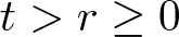 $t \gt r \ge 0$, where we used the short-hand notation (2.1). Once again, these iterated stochastic integrals in (5.22) and (5.23) are to be interpreted as multiple Wiener integrals.
We note that the drivers  $\mathbf{X}^1$,
 $\mathbf{X}^2$, and
 $\mathbf{X}^3$ in (1.11), (5.20), and (5.21), respectively, satisfy Chen’s relation (5.7) since
 $\mathbf{X}^j$’s generated by the recursive relation (5.2) satisfy a more general Chen’s relation (5.3).
 $\bullet$ Second-order driver
 $\mathbf{X}^2$ in (5.22).
We first introduce some notations. Given dyadic  $N, N_1, N_2, N_3, N_{23} \ge1$, we use
 $\textbf{N}_3$ to denote the following dyadic quintuple:
 \begin{equation}
\textbf{N}_3 = (N, N_1, N_2, N_3, N_{23}) \in (2^{\mathbb{Z}_{\ge 0}})^5.
\end{equation}
Given 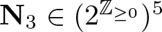 $\textbf{N}_3 \in (2^{\mathbb{Z}_{\ge 0}})^5$, define
 $ E_{\textbf{N}_3}$ by
 \begin{align}
E_{\textbf{N}_3} = \big\{(n, n_1, n_2, n_3) \in \mathbb{Z}^4:
\ & n = n_{123}, \, |n|\sim N,\cr
& |n_j|\sim N_j, \, j = 1, 2, 3, \ |n_{23}|\sim N_{23}\big\}.
\end{align}
On  $E_{\textbf{N}_3}$, we have
 \begin{equation}
\max( N, N_{23}, N_3) \sim N_{\max} := \max (N, N_1, N_2, N_3).
\end{equation}
We define  $\mathcal{D}_3$ by setting
 \begin{equation}
\mathcal{D}_3 = \left\{
\textbf{N}_3 \in (2^{\mathbb{Z}_{\ge 0}})^5: \, \textbf{N}_3\ \text{is of the form (5.24), satisfying (5.26)}
\right\}.
\end{equation}
We also denote by  $\mathcal{A}_3$ the class of functions
 $\textbf{a} = (a_1, a_2, a_3)
:(2^{\mathbb{Z}_{\ge 0}})^5 \to [0, 1)^3$ of the form:
 \begin{align*}
\textbf{a}(\textbf{N}_3) = \big(a_1(\textbf{N}_3), a_2(\textbf{N}_3), a_3(\textbf{N}_3)\big) \in [0, 1)^3
\end{align*}
for 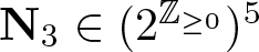 $\textbf{N}_3 \in (2^{\mathbb{Z}_{\ge 0}})^5$, satisfying
 \begin{equation}
\sum_{j = 1}^3 a_j \le 2.
\end{equation}
Proposition 5.2. Let 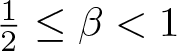 $\frac 12 \le \beta \lt 1$ and
 $s, s_0, \sigma \in \mathbb{R}$. Given
 $\phi \in \operatorname{HS}(L^2(\mathbb{T}); H^\sigma(\mathbb{T}))$ satisfying (1.8), let
 $\mathbf{X}^2$ be the second-order driver in (5.22). Given small
 $\theta \gt 0$ and
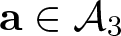 $\textbf{a} \in \mathcal{A}_3$, set
 \begin{equation}
M^{(2)}_{\beta, \sigma, s, s_0, \theta} (\textbf{a}(\textbf{N}_3))
=
\frac{N_{\max}^{\frac 12 \theta} N^{s_0-2a_1(\textbf{N}_3)\beta}}
{N_1^{\sigma} N_2^\sigma N_{23}^{2a_2(\textbf{N}_3)\beta }N_3^{s+2a_3(\textbf{N}_3)\beta}}
\end{equation}
for  $\textbf{N}_3$ of the form (5.24), where
 $N_{\max} = \max(N, N_1, N_2, N_3)$. Then, given any finite
 $p \ge 1$ and
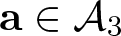 $\textbf{a} \in \mathcal{A}_3$, we have
 \begin{align}
& \big\| \| \mathbf{X}^2_{t,r} \|_{\mathcal{L}(H^{s}; H^{s_0})}
\big\|_{L^p(\Omega)}
\lesssim_\textbf{a} p \| \phi \|_{\operatorname{HS}(L^2;H^\sigma)}^2 \cr
& \qquad\qquad\quad \times
\sum_{\textbf{N}_3 \in \mathcal{D}_3}
M^{(2)}_{\beta, \sigma, s, s_0, \theta} (\text{a}(\textbf{N}_3))
(t-r)^{(2
-\sum_{j = 1}^3 a_j (\textbf{N}_3))\beta}
\end{align}
for any 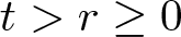 $t \gt r\ge 0$. Note that the right-hand side of (5.30) is not a priori finite.
Furthermore, suppose that the following holds for a given choice of 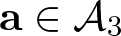 $\textbf{a} \in \mathcal{A}_3$:
(i)
$M^{(2)}_{\beta, \sigma, s, s_0, \theta} (\textbf{a}(\textbf{N}_3))$ in (5.29) is summable:
(5.31)\begin{equation}
\sum_{\textbf{N}_3 \in \mathcal{D}_3}
M^{(2)}_{\beta, \sigma, s, s_0, \theta} (\textbf{a}(\textbf{N}_3)) \lt \infty,
\end{equation}
(ii) there exists
$0 \lt \gamma \lt 1$ such that
(5.32)\begin{equation}
\inf_{\textbf{N}_3\in \mathcal{D}_3}\bigg(2
-\sum_{j = 1}^3 a_j (\textbf{N}_3)\bigg)\beta \gt \gamma,
\end{equation}
(iii) for the choice of
$\gamma$ in (ii), the bound (4.16) for the first-order driver $\mathbf{X}^1$ holds.


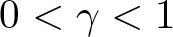


Then, we have
 \begin{equation}
\big\| \| \mathbf{X}^2 \|_{C^{\gamma}_{2,T} \mathcal{L}(H^s;H^{s_0})} \big\|_{L^p(\Omega)} \lesssim_T p \| \phi \|_{{\operatorname{HS}} (L^2; H^\sigma)}^2
\end{equation}
for any finite  $p \ge 1$ and
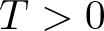 $T \gt 0$. In particular, there exists a version of
 $\mathbf{X}^2$ such that
 \begin{equation*}\mathbf{X}^2 \in C^{\gamma}_{2,T} \mathcal{L}(H^s(\mathbb{T});H^{s_0}(\mathbb{T})),\end{equation*}
almost surely.
In the next subsection, we make a suitable choice of 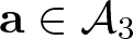 $\textbf{a} \in \mathcal{A}_3$, guaranteeing (5.31) and (5.32).
Proof of Proposition 5.2
It suffices to prove the bound (5.30), since the bound (5.33) follows from (5.30), (5.31), (5.32), and [Reference Gubinelli and Tindel19, Lemma 3.8] with (5.7) and (4.16) for  $\mathbf{X}^1$. Here, we need (4.16) for
 $\mathbf{X}^1$, since [Reference Gubinelli and Tindel19, Lemma 3.8] requires a bound on
 $\widetilde {\delta} \mathbf{X}^2
= \mathbf{X}^1 \mathbf{X}^1$ (see (5.7)).
Fix 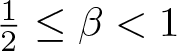 $\frac 12 \le \beta \lt 1$ and
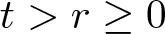 $t \gt r \ge 0$. From (5.22), we have
 \begin{equation}
{\mathcal{F}}_x\big( \langle \nabla \rangle^{s_0} \mathbf{X}^2_{t,r} \langle \nabla \rangle^{-s} f\big) (n)
= \sum_{n_3 \in \mathbb{Z}} \widehat f(n_3) I_2 [ \mathfrak{h}^2_{nn_3}(n_A) \mathfrak{g}^2_{nn_3}(t_A,n_A) ],
\end{equation}
where  $I_2$ denotes the multiple Wiener integral (see §3.1). Here, with
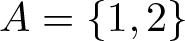 $A = \{1, 2\}$,
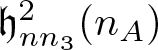 $\mathfrak{h}^2_{nn_3}(n_A) $ and
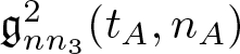 $\mathfrak{g}^2_{nn_3}(t_A, n_A) $ are defined by
 \begin{align}
\mathfrak{h}^2_{n n_3}(n_A) & =
\mathbf 1_{n=n_{123}}
\cdot
\frac {\langle n \rangle^{s_0 }} {\langle n_3 \rangle^s }\phi_{n_1}
\phi_{n_2}, \cr
\mathfrak{g}^2_{nn_3} (t_A, n_A) &=
\mathfrak{g}_{nn_3}^{2, t, r} (t_A, n_A) =
\mathbf 1_{r \le t_2 \le t_1\le t}\cr
& \quad \times
e^{-(t-t_1)\langle n \rangle^2}
e^{-(t_1-t_2)\langle n_{23} \rangle^2}
e^{- (t_2-r)\langle n_3 \rangle^2}.
\end{align}
Given 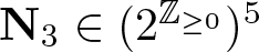 $\textbf{N}_3 \in (2^{\mathbb{Z}_{\ge 0}})^5$ of the form (5.24), we set
 \begin{align}
\mathfrak{h}^{2, \textbf{N}_3}_{n n_3}(n_A)
& = \mathbf 1_{E_{\textbf{N}_3}}
\cdot
\mathfrak{h}^2_{n n_3}(n_A), \cr
\mathfrak{g}^{2, \textbf{N}}_{nn_3} (t_A, n_A)
& = \mathbf 1_{E_{\textbf{N}_3}}
\cdot
\mathfrak{g}^2_{nn_3} (t_A, n_A),
\end{align}
where  $ E_{\textbf{N}_3}$ is as in (5.25). Then, given any
 $\theta \gt 0$, it follows from (5.34), (5.35), (5.36), and the random tensor estimate (Lemma 3.5) that
 \begin{align}
\big\| & \| \mathbf{X}^2_{t,r} \|_{\mathcal{L}(H^s;H^{s_0})} \big\|_{L^p(\Omega)}
= \big\| \| \langle \nabla \rangle^{s_0} \mathbf{X}^2_{t,r}\langle \nabla \rangle^{-s} \|_{\mathcal{L}(L^2;L^2)} \big\|_{L^p(\Omega)}\cr
& = \big\| \| I_2[ \mathfrak{h}^2_{nn_3}(n_A) \mathfrak{g}^2_{nn_3}(t_A, n_A) ] \|_{\ell^2_{n_3} \to \ell^2_n} \big\|_{L^p(\Omega)}\cr
& \le \sum_{\textbf{N}_3\in \mathcal{D}_3}
\big\| \|
I_2[ \mathfrak{h}^{2, \textbf{N}_3}_{nn_3}(n_A) \mathfrak{g}^{2, \textbf{N}_3}_{nn_3}(t_A, n_A)] \|_{\ell^2_{n_3} \to \ell^2_n} \big\|_{L^p(\Omega)}\cr
& \lesssim
p
\sum_{\textbf{N}_3\in \mathcal{D}_3}
\frac{N_{\max}^{\frac 12 \theta} N^{\theta s_0}}
{N_1^{\theta\sigma} N_2^{\theta \sigma} N_3^{\theta s} }
\|\phi\|_{\operatorname{HS}(L^2; H^\sigma)}^{2\theta}\cr
& \quad\times
\| \mathfrak{g}^{2, \textbf{N}_3}_{nn_3} (t_A, n_A)\|_{\ell^\infty_{nn_3n_A}\mathscr{H}^\beta_{t_A} }
\Big(\max_{(B, C)} \| \mathfrak{h}^{2, \textbf{N}_3}_{nn_3}(n_A)\|_{n_3n_B \to nn_C} \Big)^{1-\theta}
\end{align}
for any finite  $p \ge 1$, where
 $\mathcal{D}_3$ is as in (5.27),
 $N_{\max} = \max(N, N_1, N_2, N_3)$,
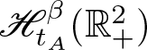 $\mathscr{H}^\beta_{t_A}(\mathbb{R}^2_+)$ is as in (3.3), and the maximum on the last factor in (5.37) is taken over all partitions
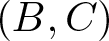 $(B, C)$ of
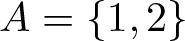 $A = \{1, 2\}$:
 \begin{equation*}n_1 n_2 n_3 \to n , \qquad
n_1 n_3 \to n n_2,
\qquad n_2 n_3 \to nn_1,
\qquad \text{and}\qquad
n_3 \to nn_1 n_2. \end{equation*}
From (5.35), (5.36), and Cauchy–Schwarz’s inequality with (1.9), we have
 \begin{align}
& \| \mathfrak{h}^{2, \textbf{N}_3}_{nn_3}(n_A)\|_{n_1n_2n_3 \to n} \cr
&\quad \sim
\frac{N^{s_0}}{N_3^s }
\sup_{\|f\|_{\ell^2_{n_1 n_2 n_3}}
= \|g\|_{\ell^2_{n}} = 1}
\bigg|
\sum_{n, n_1, n_2, n_3 \in \mathbb{Z}}
\mathbf 1_{E_{\textbf{N}_3}}
\phi_{n_1}\phi_{n_2} f_{n_1 n_2 n_3} g_{n}\bigg|\cr
&\quad \lesssim
\frac{N^{s_0}}{N_1^\sigma N_2^\sigma N_3^s}
\|\phi\|_{\operatorname{HS}(L^2; H^\sigma)}^2.
\end{align}
A similar computation yields
 \begin{equation}
\max_{(B, C)} \| \mathfrak{h}^{2, \textbf{N}_3}_{nn_3}(n_A)\|_{n_3n_B \to nn_C}
\lesssim
\frac{N^{s_0}}{N_1^\sigma N_2^\sigma N_3^s}
\|\phi\|_{\operatorname{HS}(L^2; H^\sigma)}^2.
\end{equation}
From (3.3) and Sobolev’s inequality (separately applied to each of the  $t_1$- and
 $t_2$-variables), we have
 \begin{align}
\| \mathfrak{g}^2_{nn_3} (t_A, n_A)\|_{\ell^\infty_{nn_3n_A} \mathscr{H}_{t_A}^\beta}
& =
\| \mathfrak{g}^2_{nn_3} (t_A, n_A)\|_{\ell^\infty_{nn_3n_A} \dot H_{t_A}^{\frac 12 - \beta}}\cr
& \lesssim
\| \mathfrak{g}^2_{nn_3} (t_A, n_A)\|_{\ell^\infty_{nn_3n_A} L^\frac 1\beta_{t_A}}.
\end{align}
By applying the bound on  $J^1$ in (4.27) and another change of variables with (4.26), we have
 \begin{align}
\| & \mathfrak{g}^2_{nn_3} (t_A, n_A)\|_{L^\frac 1\beta_{t_A} }^\frac 1 \beta
= J^2_{t, r}(n, n_{23}, n_3)\cr
: \!& = \int_r^t
e^{-\beta^{-1}(t-t_1)\langle n \rangle^2}
\int_r^{t_1}
e^{-\beta^{-1}(t_1-t_2)\langle n_{23} \rangle^2}
e^{- \beta^{-1}(t_2-r)\langle n_3 \rangle^2}dt_2
dt_1 \cr
& = \int_r^t
e^{-\beta^{-1}(t-t_1)\langle n \rangle^2}
J^1_{t_1, r}(n_{23}, n_3)
dt_1 \cr
& \lesssim_{\beta, a_1, a_2, a_3}
\langle n \rangle^{-2a_1}\langle n_{23} \rangle^{-2a_2}
\langle n_3 \rangle^{-2a_3}\cr
& \quad \times \int_r^t (t - t_1)^{-a_1}
(t_1- r)^{1-a_2- a_3} dt_1\cr
&
\sim_{a_1, a_2, a_3}
(t-r)^{2-\sum_{j = 1}^3 a_j }
\langle n \rangle^{-2a_1}\langle n_{23} \rangle^{-2a_2}
\langle n_3 \rangle^{-2a_3}.
\end{align}
uniformly in  $n, n_2, n_3 \in \mathbb{Z}$ and
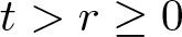 $t \gt r\ge 0$, provided that
 $0 \le a_1, a_2, a_3 \lt 1$, satisfying (5.28). Hence, from (5.40) and (5.41), we have
 \begin{equation}
\| \mathfrak{g}^{2, \textbf{N}_3}_{nn_3} (t_A, n_A)\|_{L^\frac 1\beta_{t_A} } \lesssim_{a_1, a_2, a_3} (t-r)^{(2
-\sum_{j = 1}^3 a_j )\beta}N^{-2a_1\beta}
N_{23}^{-2a_2\beta}N_{3}^{-2a_3\beta},
\end{equation}
uniformly in  $(n, n_1, n_2, n_3) \in E_{\textbf{N}_3}$,
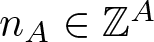 $n_A \in \mathbb{Z}^A$,
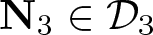 $\textbf{N}_3 \in \mathcal{D}_3$, and
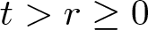 $t \gt r\ge 0$.
Therefore, putting (5.37), (5.39), and (5.42) together with (5.29), we obtain the desired bound (5.30).
 $\bullet$ Third-order driver
 $\mathbf{X}^3$ in (5.23).
Given dyadic  $N, N_1, N_2, N_3, N_4, N_{234}, N_{23} \ge1$, we use
 $\textbf{N}_4$ to denote the following dyadic septuple:
 \begin{equation}
\textbf{N}_4 = (N, N_1, N_2, N_3, N_4, N_{234}, N_{34}) \in (2^{\mathbb{Z}_{\ge 0}})^7.
\end{equation}
Given 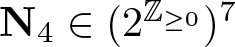 $\textbf{N}_4 \in (2^{\mathbb{Z}_{\ge 0}})^7$, define
 $ E_{\textbf{N}_4}$ by
 \begin{align}
E_{\textbf{N}_4} = \big\{(n, n_1, n_2, n_3, n_4) \in \mathbb{Z}^5:
\ & n = n_{1234}, \, |n|\sim N,\cr
& |n_j|\sim N_j, \, j = 1, \dots, 4,\cr
& |n_{234}|\sim N_{234},
\, |n_{34}|\sim N_{34}
\big\}.
\end{align}
On  $E_{\textbf{N}_4}$, we have
 \begin{equation}
\max( N, N_{234}, N_{34}, N_4) \sim N_{\max} : = \max (N, N_1, N_2, N_3, N_4).
\end{equation}
We define  $\mathcal{D}_4$ by setting
 \begin{equation}
\mathcal{D}_4 = \left\{
\textbf{N}_4 \in (2^{\mathbb{Z}_{\ge 0}})^7: \, \textbf{N}_4\ \text{is of the form (5.43), satisfying (5.45)}
\right\}.
\end{equation}
We also denote by  $\mathcal{A}_4$ the class of functions
 $\textbf{a} = (a_1, a_2, a_3, a_4)
:(2^{\mathbb{Z}_{\ge 0}})^7 \to [0, 1)^4$ of the form:
 \begin{equation}
\textbf{a}(\textbf{N}_4) = \big(a_1(\textbf{N}_4), a_2(\textbf{N}_4), a_3(\textbf{N}_4), a_4(\textbf{N}_4)\big) \in [0, 1)^4
\end{equation}
for  $\textbf{N}_4 \in (2^{\mathbb{Z}_\ge 0})^7$, satisfying
 \begin{equation}
\sum_{j = 1}^4 a_j \le 3.
\end{equation}
Proposition 5.3. Let 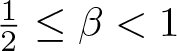 $\frac 12 \le \beta \lt 1$ and
 $s, s_0, \sigma \in \mathbb{R}$. Given
 $\phi \in \operatorname{HS}(L^2(\mathbb{T}); H^\sigma(\mathbb{T}))$ satisfying (1.8), let
 $\mathbf{X}^3$ be the third-order driver in (5.23). Given small
 $\theta \gt 0$ and
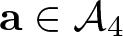 $\textbf{a} \in \mathcal{A}_4$, set
 \begin{equation}
M^{(3)}_{\beta, \sigma, s, s_0, \theta} (\textbf{a}(\textbf{N}_4))
=
\frac{N_{\max}^{\frac 12 \theta} N^{s_0- 2a_1(\textbf{N}_4)\beta}}
{N_1^{\sigma} N_2^\sigma N_3^\sigma N_{234}^{2a_2(\textbf{N}_4)\beta }
N_{34}^{2a_3(\textbf{N}_4)\beta }
N_4^{s+2a_4(\textbf{N}_4)\beta}}
\end{equation}
for  $\textbf{N}_4$ of the form (5.43), where
 $N_{\max} = \max(N, N_1, \dots, N_4)$. Then, given any finite
 $p \ge 1$ and
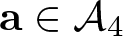 $\textbf{a} \in \mathcal{A}_4$, we have
 \begin{align}
& \big\| \| \mathbf{X}^3_{t,r} \|_{\mathcal{L}(H^{s}; H^{s_0})}
\big\|_{L^p(\Omega)}
\lesssim_\textbf{a} p^\frac 32 \| \phi \|_{\operatorname{HS}(L^2;H^\sigma)}^3 \cr
& \quad\times
\sum_{\textbf{N}_4 \in \mathcal{D}_4}
M^{(3)}_{\beta, \sigma, s, s_0, \theta} (\textbf{a}(\textbf{N}_4))
(t-r)^{(3
-\sum_{j = 1}^4 a_j (\textbf{N}_4))\beta}
\end{align}
for any  $t \gt r\ge 0$, uniformly in
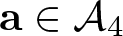 $\textbf{a} \in \mathcal{A}_4$.
Furthermore, suppose that the following holds for a given choice of 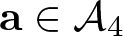 $\textbf{a} \in \mathcal{A}_4$:
(i)
$M^{(3)}_{\beta, \sigma, s, s_0, \theta} (\textbf{a}(\textbf{N}_4))$ in (5.49) is summable:
(5.51)\begin{equation}
\sum_{\textbf{N}_4 \in \mathcal{D}_4}
M^{(3)}_{\beta, \sigma, s, s_0, \theta} (\textbf{a}(\textbf{N}_4)) \lt \infty,
\end{equation}
(ii) there exists
$0 \lt \gamma \lt 1$ such that
(5.52)\begin{equation}
\inf_{\textbf{N}_4\in \mathcal{D}_4}\bigg(3
-\sum_{j = 1}^4 a_j (\textbf{N}_4)\bigg)\beta \gt \gamma,
\end{equation}
(iii) for the choice of
$\gamma$ in (ii), the bounds (4.16) and (5.33) for $\mathbf{X}^1$ and $\mathbf{X}^2$, respectively, hold.


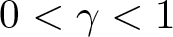


Then, we have
 \begin{equation}
\big\| \| \mathbf{X}^3 \|_{C^{\gamma}_{2,T} \mathcal{L}(H^s;H^{s_0})} \big\|_{L^p(\Omega)} \lesssim_T p^\frac 32 \| \phi \|_{{\operatorname{HS}} (L^2; H^\sigma)}^3
\end{equation}
for any finite  $p \ge 1$ and
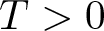 $T \gt 0$. In particular, there exists a version of
 $\mathbf{X}^3$ such that
 \begin{equation*}\mathbf{X}^3 \in C^{\gamma}_{2,T} \mathcal{L}(H^s(\mathbb{T});H^{s_0}(\mathbb{T})),\end{equation*}
almost surely.
In the next subsection, we make a suitable choice of 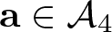 $\textbf{a} \in \mathcal{A}_4$, guaranteeing (5.51) and (5.52).
Proof of Proposition 5.3
As in the proof of Proposition 5.2, it suffices to prove the bound (5.50), since the bound (5.53) follows from (5.50), (5.51), (5.52), and [Reference Gubinelli and Tindel19, Lemma 3.8] with (5.7) and the bounds (4.16) and (5.33) for  $\mathbf{X}^1$ and
 $\mathbf{X}^2$.
Fix 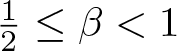 $\frac 12 \le \beta \lt 1$ and
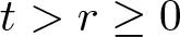 $t \gt r \ge 0$. From (5.23), we have
 \begin{equation}
{\mathcal{F}}_x\big( \langle \nabla \rangle^{s_0} \mathbf{X}^3_{t,r} \langle \nabla \rangle^{-s} f\big) (n)
= \sum_{n_4 \in \mathbb{Z}} \widehat f(n_4) I_3 [ \mathfrak{h}^3_{nn_4}(n_A) \mathfrak{g}^3_{nn_4}(t_A,n_A) ],
\end{equation}
where  $I_3$ denotes the multiple Wiener integral (see §3.1). Here, with
 $A = \{1, 2, 3\}$,
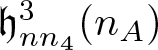 $\mathfrak{h}^3_{nn_4}(n_A) $ and
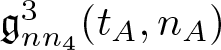 $\mathfrak{g}^3_{nn_4}(t_A, n_A)$ are defined by
 \begin{align}
\mathfrak{h}^3_{n n_4}(n_A) & =
\mathbf 1_{n=n_{1234}}
\cdot
\frac {\langle n \rangle^{s_0 }} {\langle n_4 \rangle^s }
\prod_{j = 1}^3\phi_{n_j} , \cr
\mathfrak{g}^3_{nn_4} (t_A, n_A) &=
\mathfrak{g}_{nn_4}^{3, t, r} (t_A, n_A) =
\mathbf 1_{r \le t_3 \le t_2 \le t_1\le t}\cr
& \quad \times
e^{-(t-t_1)\langle n \rangle^2}
e^{-(t_1-t_2)\langle n_{234} \rangle^2}
e^{- (t_2-t_3)\langle n_{34} \rangle^2}
e^{- (t_3-r)\langle n_4 \rangle^2}.
\end{align}
Given 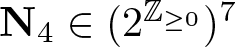 $\textbf{N}_4 \in (2^{\mathbb{Z}_{\ge 0}})^7$ of the form (5.43), we set
 \begin{align}
\mathfrak{h}^{3, \textbf{N}_4}_{n n_4}(n_A)
& = \mathbf 1_{E_{\textbf{N}_4}}
\cdot
\mathfrak{h}^3_{n n_4}(n_A), \cr
\mathfrak{g}^{3, \textbf{N}_4}_{nn_4} (t_A, n_A)
&= \mathbf 1_{E_{\textbf{N}_4}}
\cdot
\mathfrak{g}^3_{nn_4} (t_A, n_A),
\end{align}
where  $ E_{\textbf{N}_4}$ is as in (5.44). Then, given any
 $\theta \gt 0$, it follows from (5.54), (5.55), (5.56), and the random tensor estimate (Lemma 3.5) that
 \begin{align}
\big\| & \| \mathbf{X}^3_{t,r} \|_{\mathcal{L}(H^s;H^{s_0})} \big\|_{L^p(\Omega)}
= \big\| \| \langle \nabla \rangle^{s_0} \mathbf{X}^3_{t,r}\langle \nabla \rangle^{-s} \|_{\mathcal{L}(L^2;L^2)} \big\|_{L^p(\Omega)}\cr
& = \big\| \| I_3[ \mathfrak{h}^3_{nn_4}(n_A) \mathfrak{g}^3_{nn_4}(t_A, n_A) ] \|_{\ell^2_{n_4} \to \ell^2_n} \big\|_{L^p(\Omega)}\cr
& \le \sum_{\textbf{N}_4 \in \mathcal{D}_4}
\big\| \|
I_3[ \mathfrak{h}^{3, \textbf{N}_4}_{nn_4}(n_A) \mathfrak{g}^{3, \textbf{N}_4}_{nn_4}(t_A, n_A)] \|_{\ell^2_{n_4} \to \ell^2_n} \big\|_{L^p(\Omega)}\cr
& \lesssim
p^\frac 32
\sum_{\textbf{N}_4 \in \mathcal{D}_4}
\frac{N_{\max}^{\frac 12 \theta} N^{\theta s_0}}
{N_1^{\theta\sigma} N_2^{\theta \sigma} N_3^{\theta \sigma} N_4^{\theta s} }
\|\phi\|_{\operatorname{HS}(L^2; H^\sigma)}^{3\theta}\cr
& \quad\times
\| \mathfrak{g}^{3, \textbf{N}_4}_{nn_4} (t_A, n_A)\|_{\ell^\infty_{nn_4n_A}\mathscr{H}^\beta_{t_A} }
\Big(\max_{(B, C)} \| \mathfrak{h}^{3, \textbf{N}_4}_{nn_4}(n_A)\|_{n_4n_B \to nn_C} \Big)^{1-\theta}
\end{align}
for any finite  $p \ge 1$, where
 $\mathcal{D}_4$ is as in (5.46),
 $N_{\max} = \max(N, N_1, \dots, N_4)$,
 $\mathscr{H}^\beta_{t_A}(\mathbb{R}^3_+)$ is as in (3.3), and the maximum on the last factor is taken over all partitions
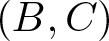 $(B, C)$ of
 $A = \{1, 2, 3\}$.
Proceeding as in (4.23) and (5.38) with Cauchy–Schwarz’s inequality, we have
 \begin{equation}
\max_{(B, C)} \| \mathfrak{h}^{3, \textbf{N}_4}_{nn_4}(n_A)\|_{n_4n_B \to nn_C}
\lesssim
\frac{N^{s_0}}{N_1^\sigma N_2^\sigma N_3^\sigma N_4^s}
\|\phi\|_{\operatorname{HS}(L^2; H^\sigma)}^3.
\end{equation}
By applying Sobolev’s inequality (separately applied to each of the  $t_1$-,
 $t_2$-, and
 $t_3$-variables) with (3.3), the bound on
 $J^2$ in (5.41), and another change of variables, we have
 \begin{align}\| & \mathfrak{g}^3_{nn_4} (t_A, n_A)\|_{\mathscr{H}_{t_A}^\beta}^\frac 1 \beta
\lesssim \| \mathfrak{g}^3_{nn_4} (t_A, n_A)\|_{L^\frac 1\beta_{t_A} }^\frac 1 \beta \cr
& = \int_r^t
\int_r^{t_1}
\int_r^{t_2}
e^{-\beta^{-1}(t-t_1)\langle n \rangle^2}
e^{-\beta^{-1}(t_1-t_2)\langle n_{234} \rangle^2} \cr
&
\quad\times e^{- \beta^{-1}(t_2-t_3)\langle n_{34} \rangle^2}
e^{- \beta^{-1}(t_3-r)\langle n_4 \rangle^2}
dt_3 dt_2
dt_1 \cr
& = \int_r^t
e^{-\beta^{-1}(t-t_1)\langle n \rangle^2}
J^2_{t_1, r}(n_{234},n_{34}, n_4)
dt_1\cr
& \lesssim_{\beta, a_1, \dots, a_4}
\langle n \rangle^{-2a_1}\langle n_{234} \rangle^{-2a_2}
\langle n_{34} \rangle^{-2a_3}
\langle n_4 \rangle^{-2a_4}\cr
& \quad \times \int_r^t (t - t_1)^{-a_1}
(t_1- r)^{2-\sum_{j =2}^4a_j} dt_1\cr
&
\sim_{a_1, \dots, a_4}
(t-r)^{3-\sum_{j = 1}^4 a_j }
\langle n \rangle^{-2a_1}\langle n_{234} \rangle^{-2a_2}
\langle n_{34} \rangle^{-2a_3}
\langle n_4 \rangle^{-2a_4}, \end{align}
uniformly in  $n, n_2, n_3, n_4 \in \mathbb{Z}$ and
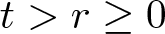 $t \gt r\ge 0$, provided that
 $0 \le a_1, \dots , a_4 \lt 1$, satisfying (5.48). Hence, we have
 \begin{align}
& \| \mathfrak{g}^{3, \textbf{N}_4}_{nn_4} (t_A, n_A)\|_{L^\frac 1\beta_{t_A} }\cr
& \quad \lesssim_{a_1, \dots, a_4}
(t-r)^{(3-\sum_{j = 1}^4 a_j )\beta }
N^{-2a_1\beta }
N_{234}^{-2a_2\beta }
N_{34}^{-2a_3\beta }
N_{4}^{-2a_4\beta},
\end{align}
uniformly in  $(n, n_1, n_2, n_3, n_4) \in E_{\textbf{N}_4}$,
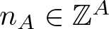 $n_A \in \mathbb{Z}^A$,
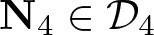 $\textbf{N}_4 \in \mathcal{D}_4$, and
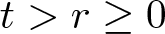 $t \gt r\ge 0$.
Therefore, putting (5.57), (5.58), and (5.60) together with (5.49), we obtain the desired bound (5.50).
5.3. Proof of Theorem 1.3
We conclude this section by presenting a proof of Theorem 1.3. More precisely, we prove that under a suitable choice of parameters, the convolution RDE (5.4) is pathwise globally well-posed.
Proof of Theorem 1.3
Let 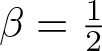 $\beta = \frac 12$ and fix
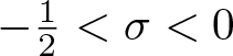 $- \frac 12 \lt \sigma \lt 0$. Given small
 $\varepsilon \gt 0$ (to be chosen later), we set
 \begin{equation}
\alpha = \frac 14 + \varepsilon\qquad \text{and}\qquad
\gamma = \frac 14 + 2\varepsilon.
\end{equation}
Part 1: We show that there exists  $ s \gt 0$ such that (5.9) holds for any
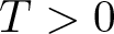 $T \gt 0$, almost surely
We first consider the first-order driver  $\mathbf{X}^1$ in (1.11). By setting
 $s_0 = s \gt 0$ and
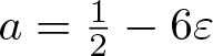 $a = \frac 12 - 6\varepsilon$, the conditions in (4.14) of Proposition 4.2 reduce to
 \begin{equation}
\sigma \gt s - \frac 12 + 6\varepsilon,
\end{equation}
which guarantees that
 \begin{equation}
\mathbf{X}^1 \in \bigcap_{k = 1}^\infty C^{\gamma}_{2,k} \mathcal{L}(H^s(\mathbb{T})),
\end{equation}
almost surely; see (4.15) and (4.16).
Next, we consider the second-order driver  $\mathbf{X}^2$ in (5.20). Given
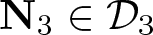 $\textbf{N}_3 \in \mathcal{D}_3$ (see (5.27)), we set
 \begin{equation}
a_{j_*}(\textbf{N}_3) = 1 - 10 \varepsilon
\end{equation}
for  $j_* \in \{1, 2, 3\}$ corresponding to the maximum of
 $N$,
 $N_{23}$, and
 $N_3$ in (5.29), and set
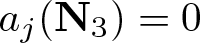 $a_j(\textbf{N}_3) = 0$ for
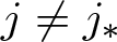 $j \ne j_*$. Then, in view of (5.26) (recall
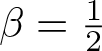 $\beta = \frac 12$), we have
 \begin{equation}
N^{-a_1(\textbf{N}_3)}
N_{23}^{- a_2(\textbf{N}_3) }N_3^{- a_3(\textbf{N}_3)}
\lesssim N_{\max}^{-1 + 10 \varepsilon}.
\end{equation}
Then, from (5.29) (with 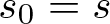 $s_0 = s$) and (5.65), we have
 \begin{align*}
\sum_{\textbf{N}_3 \in \mathcal{D}_3} M^{(2)}_{\beta, \sigma, s, s, \theta} (\textbf{a}(\textbf{N}_3))
=
\sum_{\textbf{N}_3 \in \mathcal{D}_3}
\frac{N_{\max}^{\frac 12 \theta - 1 + 10 \varepsilon} N^{s}}
{N_1^{\sigma} N_2^\sigma N_3^{s}} \lt \infty,
\end{align*}
provided that
 \begin{equation}
\sigma \gt \frac 12 s - \frac 12 + \frac 14 \theta + 5 \varepsilon.
\end{equation}
As a result, it follows from Proposition 5.2 with (5.64) and (5.61) that, given any finite  $p \ge 1$, we have
 \begin{align*}
\big\| \| \mathbf{X}^2_{t,r} \|_{\mathcal{L}(H^{s})}
\big\|_{L^p(\Omega)}
\lesssim p \| \phi \|_{\operatorname{HS}(L^2;H^\sigma)}^2
(t-r)^{2\gamma + \varepsilon}
\end{align*}
for any 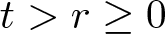 $t \gt r\ge 0$ and thus
 \begin{equation}
\mathbf{X}^2 \in \bigcap_{k = 1}^\infty C^{2\gamma}_{2,k} \mathcal{L}(H^s(\mathbb{T})),
\end{equation}
almost surely; see (5.30) and (5.33).
We now consider the third-order driver  $\mathbf{X}^3$ in (5.21). Given
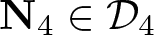 $\textbf{N}_4 \in \mathcal{D}_4$ (see (5.46)), we choose
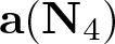 $\textbf{a}(\textbf{N}_4)$ in (5.47) such that
 \begin{equation}
\sum_{j = 1}^4 a_j(\textbf{N}_4) = \frac 32 - 14\varepsilon.
\end{equation}
 $\bullet$ Case 1:
 $N \vee N_{234} \sim N_{\max}$.
In this case, we set  $a_j(\textbf{N}_4) = 1- 13\varepsilon$ for
 $j = 1$ if
 $N \ge N_{234}$ and
 $j = 2$ if
 $N \lt N_{234}$. On
 $E_{\textbf{N}_4}$ defined in (5.44), we have
 $N_{34} \vee N_4 \gt rsim N_{3}$. Then, we set
 $a_j(\textbf{N}_4) = \frac 12 - \varepsilon$ for
 $j = 3$ if
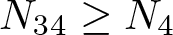 $N_{34} \ge N_{4}$ and
 $j = 4$ if
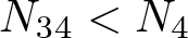 $N_{34} \lt N_{4}$. We set
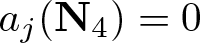 $a_j(\textbf{N}_4) = 0$ for the remaining
 $j$’s. Then, we have
 \begin{equation}
\frac{N_{\max}^{\frac 12 \theta} N^{- a_1(\textbf{N}_4)}}
{N_3^\sigma N_{234}^{a_2(\textbf{N}_4) }
N_{34}^{a_3(\textbf{N}_4) }
N_4^{a_4(\textbf{N}_4)}}
\lesssim N_{\max}^{\frac 12 \theta - 1 + 13\varepsilon},
\end{equation}
provided that  $\varepsilon \gt 0$ is sufficiently small such that
 \begin{equation}
\sigma \ge - \frac 12 + \varepsilon.
\end{equation}
 $\bullet$ Case 2:
 $N, N_{234} \ll N_{\max}$.
In this case, we have  $N_{34} \vee N_4 \sim N_{\max}$. We set
 $a_j(\textbf{N}_4) = 1- 13\varepsilon$ for
 $j = 3$ if
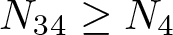 $N_{34} \ge N_{4}$ and
 $j = 4$ if
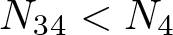 $N_{34} \lt N_{4}$. On
 $E_{\textbf{N}_4}$ defined in (5.44), we have
 $N \vee N_{234} \gt rsim N_{1}$. Then, we set
 $a_j(\textbf{N}_4) = \frac 12 - \varepsilon$ for
 $j = 1$ if
 $N \ge N_{234}$ and
 $j = 2$ if
 $N \lt N_{234}$. We set
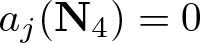 $a_j(\textbf{N}_4) = 0$ for the remaining
 $j$’s. Then, we have
 \begin{equation}
\frac{N_{\max}^{\frac 12 \theta} N^{- a_1(\textbf{N}_4)}}
{N_1^\sigma N_{234}^{a_2(\textbf{N}_4) }
N_{34}^{a_3(\textbf{N}_4) }
N_4^{a_4(\textbf{N}_4)}}
\lesssim N_{\max}^{\frac 12 \theta - 1 + 13\varepsilon},
\end{equation}
provided that (5.70) holds.
From (5.49), (5.69), and (5.71), we have
 \begin{align*}
\sum_{\textbf{N}_4 \in \mathcal{D}_4} M^{(3)}_{\beta, \sigma, s, s, \theta} (\textbf{a}(\textbf{N}_4)) \lt \infty,
\end{align*}
provided that
 \begin{equation}
\sigma \gt \frac 12 s - \frac 12 + \frac 14 \theta + \frac{13} 2 \varepsilon.
\end{equation}
As a result, it follows from Proposition 5.3 with (5.68) and (5.61) that, given any finite  $p \ge 1$, we have
 \begin{align*}
\big\| \| \mathbf{X}^3_{t,r} \|_{\mathcal{L}(H^{s})}
\big\|_{L^p(\Omega)}
\lesssim p^\frac 32 \| \phi \|_{\operatorname{HS}(L^2;H^\sigma)}^3
(t-r)^{3\gamma + \varepsilon}
\end{align*}
for any 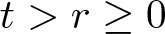 $t \gt r\ge 0$ and thus
 \begin{equation}
\mathbf{X}^3 \in \bigcap_{k = 1}^\infty C^{3\gamma}_{2,k} \mathcal{L}(H^s(\mathbb{T})),
\end{equation}
almost surely; see (5.50) and (5.53).
 $\bullet$ Summary: Let
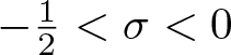 $- \frac 12 \lt \sigma \lt 0$. Then, there exists small
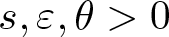 $s, \varepsilon, \theta \gt 0$ such that (5.62), (5.66), (5.70), and (5.72) hold. Hence, it follows from (5.63),(5.67), and (5.73) that there exists
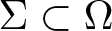 $\Sigma \subset \Omega$ with
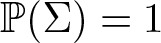 $\mathbb{P}(\Sigma) = 1$ such that, for each
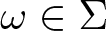 $\omega \in \Sigma$ and
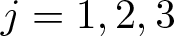 $j = 1,2, 3$, we have
 \begin{align*}
\mathbf{X}^j= \mathbf{X}^j (\omega)
\in \bigcap_{k = 1}^\infty C^{j\gamma }_{2,k} \mathcal{L}(H^s(\mathbb{T})).
\end{align*}
In the following, we fix 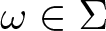 $\omega \in \Sigma$ and often suppress dependence on
 $\omega$.
Part 2: In the following, we briefly discuss pathwise well-posedness of the convolution RDE (5.4).
Let 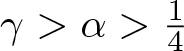 $\gamma \gt \alpha \gt \frac 14$ be as in (5.61) and fix
 $0 \lt T \le 1$ (to be chosen later). Given
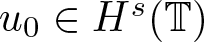 $u_0 \in H^s(\mathbb{T})$, define
 $\mathcal{D}_{\mathbf{X}^1, \mathbf{X}^2, T}^{\alpha, \gamma, u_0}(H^s(\mathbb{T}))$ to be the subclass of
 $\mathcal{D}_{\mathbf{X}^1, \mathbf{X}^2, T}^{\alpha, \gamma}(H^s(\mathbb{T}))$ defined in Definition 5.1 (i) such that
 $u|_{t = 0} = u^1|_{t = 0} = u^2|_{t = 0} = u_0$. Given
 $\mathbf{u} = (u, u^1, u^2)
\in \mathcal{D}_{\mathbf{X}^1, \mathbf{X}^2, T}^{\alpha, \gamma, u_0}(H^s(\mathbb{T}))$, satisfying
 \begin{align}
\widehat {\delta} u & = \mathbf{X}^1 (u^1) + \mathbf{X}^2(u^2) + R^{0, \mathbf{u}}, \cr
\widehat {\delta} u^1 & = \mathbf{X}^1 (u^2) + R^{1, \mathbf{u}}
\end{align}
for some  $R^{0, \mathbf{u}} \in C_{2, T}^{\alpha + 2\gamma}H^s(\mathbb{T})$ and
 $R^{1, \mathbf{u}} \in C_{2, T}^{\alpha + \gamma}H^s(\mathbb{T})$ (with the short-hand notation (2.7)), define the process
 $z = z(u, u^1, u^2)$ by
 \begin{align}
z(t)
& = S(t) u_0 + \mathcal{I}^{\overline{\mathbf{X}}}(u)(t)\cr
& = S(t) u_0 +
\Big((\operatorname{Id} - \widehat \Lambda \widehat {\delta})
\big[\mathbf{X}^1 (u)
+ \mathbf{X}^2 (u^1)
+ \mathbf{X}^3 (u^2) \big] \Big)_{t, 0}.
\end{align}
See (5.18). Then, from the convolution sewing lemma (Lemma 4.1) with (5.14) and (5.15) (recall that  $\alpha + 3\gamma \gt 1$), we have
 \begin{align}
\widehat {\delta} z
& = (\operatorname{Id} - \widehat \Lambda \widehat {\delta})
\big[\mathbf{X}^1 (u)
+ \mathbf{X}^2 (u^1)
+ \mathbf{X}^3 (u^2) \big] \cr
& =
\mathbf{X}^1 (u)
+ \mathbf{X}^2 (u^1) + R^{0, \mathbf{z}},
\end{align}
where  $R^{0, \mathbf{z}}$ is given by
 \begin{align}
R^{0, \mathbf{z}}
& =
\mathbf{X}^3 (u^2)
- \widehat \Lambda \widehat {\delta}
\big[\mathbf{X}^1 (u)
+ \mathbf{X}^2 (u^1)
+ \mathbf{X}^3 (u^2) \big] \cr
& =
\mathbf{X}^3 (u^2)
+ \widehat \Lambda \big[\mathbf{X}^1(R^{0, \mathbf{u}}) +
\mathbf{X}^2(R^{1, \mathbf{u}})
+ \mathbf{X}^3(\widehat {\delta} u^2)\big].
\end{align}
Here, the second equality follows from (5.14) and (5.15). By comparing (5.76) with (5.5), we can take the first Gubinelli derivative  $z^1$ of
 $z$ to be
 \begin{equation}
z^1 = u.
\end{equation}
Note that there is no a priori uniqueness of the Gubinelli derivative under smooth perturbation. Then, from (5.78) and (5.74), we have
 \begin{equation}
\widehat {\delta} z^1 = \mathbf{X}^1 (u^1) + R^{1, \mathbf{z}},
\end{equation}
where  $R^{1, \mathbf{z}}$ is given by
 \begin{equation}
R^{1, \mathbf{z}}
= \mathbf{X}^2(u^2) + R^{0, \mathbf{u}}.
\end{equation}
By comparing (5.79) with (5.5), we can take the second Gubinelli derivative  $z^2$ of
 $z$ to be
 \begin{equation}
z^2 = u^1.
\end{equation}
Hence, we define a map  ${\Gamma}$ on
 $\mathcal{D}_{\mathbf{X}^1, \mathbf{X}^2, T}^{\alpha, \gamma, u_0}(H^s(\mathbb{T}))$ by setting
 \begin{align}
{\Gamma}(\mathbf{u}) = {\Gamma}(u, u^1, u^2)
& = \mathbf{z} = (z, z^1, z^2)\cr
& = (z, u, u^1),
\end{align}
where  $z$ is as in (5.75) and (5.76) and the last equality holds thanks to (5.78) and (5.81).
From (5.78), (2.11), (2.12), (2.10), and (5.74) with  $z^1|_{t = 0} = u|_{t = 0} = u_0$, we have
 \begin{align}
\|z^1\|_{\widehat{\mathcal{C}}^\alpha_T H^s_x}
& \lesssim \| \widehat {\delta} u \|_{C^\alpha_{2, T} H^s_x} + \|u_0\|_{H^s}\cr
& \le T^{\gamma - \alpha}\|\mathbf{X}^1\|_{C^\gamma_{2, T} \mathcal{L}(H^s)} \|u^1\|_{L^\infty_TH^s_x} \cr
& \quad +
T^{2\gamma - \alpha}\|\mathbf{X}^2\|_{C^{2\gamma}_{2, T} \mathcal{L}(H^s)} \|u^2\|_{L^\infty_TH^s_x}\cr
& \quad + T^{2\gamma} \|R^{0, \mathbf{u}}\|_{C^{\alpha+2\gamma}_{2, T} H^s_x}
+ \|u_0\|_{H^s}\cr
& \le T^{\gamma - \alpha}\|\mathbf{X}^1\|_{C^\gamma_{2, T} \mathcal{L}(H^s)} \|u^1\|_{\widehat{\mathcal{C}}_T^\alpha H^s_x}\cr
& \quad +
T^{2\gamma - \alpha}\|\mathbf{X}^2\|_{C^{2\gamma}_{2, T} \mathcal{L}(H^s)} \|u^2\|_{\widehat{\mathcal{C}}_T^\alpha H^s_x}\cr
& \quad + T^{2\gamma} \|R^{0, \mathbf{u}}\|_{C^{\alpha+2\gamma}_{2, T} H^s_x}
+ \|u_0\|_{H^s}.
\end{align}
Similarly, from (5.81) and (5.74) with  $z^2|_{t = 0} = u^1|_{t = 0} = u_0$, we have
 \begin{align}
\|z^2\|_{\widehat{\mathcal{C}}^\alpha_T H^s_x}
& \lesssim \| \widehat {\delta} u^1 \|_{C^\alpha_{2, T} H^s_x} + \|u_0\|_{H^s}\cr
& \le T^{\gamma - \alpha}\|\mathbf{X}^1\|_{C^\gamma_{2, T} \mathcal{L}(H^s)} \|u^2\|_{L^\infty_TH^s_x} \cr
& \quad +
T^{\gamma} \|R^{1, \mathbf{u}}\|_{C^{\alpha+\gamma}_{2, T} H^s_x}
+ \|u_0\|_{H^s}\cr
& \le T^{\gamma - \alpha}
\|\mathbf{X}^1\|_{C^\gamma_{2, T} \mathcal{L}(H^s)} \|u^2\|_{\widehat{\mathcal{C}}_T^\alpha H^s_x} \cr
& \quad + T^{\gamma} \|R^{1, \mathbf{u}}\|_{C^{\alpha+\gamma}_{2, T} H^s_x}
+ \|u_0\|_{H^s}.
\end{align}
From (5.77) and the convolution sewing lemma (Lemma 4.1), we have
 \begin{align}
\|R^{0, \mathbf{z}}\|_{C^{\alpha + 2\gamma}_{2, T}H^s_x}
& \lesssim
T^{\gamma - \alpha} \|\mathbf{X}^3\|_{C^{3\gamma}_{2, T} \mathcal{L}(H^s)} \|u^2\|_{L^\infty_T H^s_x} \cr
& \quad +
T^\gamma \Big\|\widehat \Lambda \big[\mathbf{X}^1(R^{0, \mathbf{u}}) +
\mathbf{X}^2(R^{1, \mathbf{u}})
+ \mathbf{X}^3(\widehat {\delta} u^2)\big] \Big\|_{C^{\alpha + 3\gamma}_{2, T}H^s_x}\cr
& \le T^{\gamma - \alpha} \|\mathbf{X}^3\|_{C^{3\gamma}_{2, T} \mathcal{L}(H^s)} \|u^2\|_{\widehat{\mathcal{C}}_T^\alpha H^s_x} \cr
& \quad + T^\gamma \Big(\|\mathbf{X}^1\|_{C^{\gamma}_{2, T} \mathcal{L}(H^s)}
\|R^{0, \mathbf{u}}\|_{C^{\alpha+2\gamma}_{2, T} H^s_x} \cr
&
+ \|\mathbf{X}^2\|_{C^{2\gamma}_{2, T} \mathcal{L}(H^s)}
\|R^{1, \mathbf{u}}\|_{C^{\alpha+\gamma}_{2, T} H^s_x}\cr
&
+ \|\mathbf{X}^3\|_{C^{3\gamma}_{2, T} \mathcal{L}(H^s)}
\| u^2 \|_{\widehat{\mathcal{C}}_T^\alpha H^s_x}\Big).
\end{align}
From (5.80), we have
 \begin{align}
\|R^{1, \mathbf{z}}\|_{C^{\alpha + \gamma}_{2, T}H^s_x}
& \le T^{\gamma-\alpha}
\|\mathbf{X}^2\|_{C^{2\gamma}_{2, T} \mathcal{L}(H^s)}
\|u^2\|_{L^\infty_T H^s_x}
+ T^\gamma \|R^{0, \mathbf{u}}\|_{C^{\alpha + 2\gamma}_{2, T}H^s_x}\cr
& \le T^{\gamma-\alpha}
\|\mathbf{X}^2\|_{C^{2\gamma}_{2, T} \mathcal{L}(H^s)}
\|u^2\|_{\widehat{\mathcal{C}}_T^\alpha H^s_x}
+ T^\gamma \|R^{0, \mathbf{u}}\|_{C^{\alpha + 2\gamma}_{2, T}H^s_x}.
\end{align}
Therefore, putting (5.83), (5.84), (5.85), and (5.86) together with analogous difference estimates, we see that the map  ${\Gamma}$ defined in (5.82) is a contraction on
 $ \mathcal{D}_{\mathbf{X}^1, \mathbf{X}^2, T}^{\alpha, \gamma, u_0}(H^s(\mathbb{T}))$ (see (5.6)), by choosing
 \begin{equation}
T = T\Big( \|\mathbf{X}^1(\omega) \|_{C^{\gamma}_{2, 1} \mathcal{L}(H^s)},
\|\mathbf{X}^2(\omega) \|_{C^{2\gamma}_{2, 1} \mathcal{L}(H^s)},
\|\mathbf{X}^3(\omega) \|_{C^{3\gamma}_{2, 1} \mathcal{L}(H^s)}
\Big) \gt 0
\end{equation}
sufficiently small. Since a required argument is standard, we omit details. See, for example, [Reference Chapouto, Gubinelli, Li, Li and Oh4, Subsection 4.4] for details of such an argument (in the context of a nonlinear YDE with a rough perturbation).
By the Banach fixed point theorem, there exists a unique fixed point  $\mathbf{u} = (u, u^1, u^2) \in
\mathcal{D}_{\mathbf{X}^1, \mathbf{X}^2, T}^{\alpha, \gamma, u_0}(H^s(\mathbb{T}))$ for
 ${\Gamma}$. In particular, from (5.82), we have
 \begin{equation}
z = u = u^1 = u^2,
\end{equation}
and hence it follows from (5.75) that  $u$ is a unique solution to the convolution RDE (5.4). This proves pathwise local well-posedness.
Pathwise global well-posedness follows as in the Young case by noting that the local existence time in (5.87) does not depend on the initial data, allowing us to iterate the local-in-time argument. We omit details.
Acknowledgements
The authors would also like to express their gratitude to the anonymous referees for the helpful comments which improved the quality of the paper.
Funding statement
T.O. was supported by the European Research Council (grant no. 864138 ‘SingStochDispDyn’) and also acknowledges support from the NSFC (grant no. W2531005). Y.S. is grateful to the financial supports of the National Key R&D Program of China (grant no. 2022YFA1006300) and the NSFC (grant no. 12426205, no. 12271030).


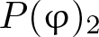

 Open access

