I. INTRODUCTION
The correlation between residual stresses and data from instrumented indentation testing (IIT) has been the subject of a significant number of publication in the past 15 years. In general, these publications may be divided into analysis on how residual stresses affect the load–displacement curve (also called the direct method) and analysis on how to calculate the value of residual stress based on instrumented indentation data (inverse method).
A. Effects of residual stress on IIT
Contributions toward the analysis of the effects of residual stresses on instrumented indentation data may be found in the works by Tsui et al.Reference Tsui, Oliver and Pharr1 and Bolshakov et al.Reference Bolshakov, Oliver and Pharr2 In the first case,Reference Tsui, Oliver and Pharr1 results initially confirmed a trend published in the literature,Reference Sines and Carlson3 according to which tensile residual stresses decrease the value of hardness measured during, e.g., Rockwell B tests, while compressive residual stresses are responsible for an increase in hardness values. In this case, the effects are more evident when the stresses are tensile. Tsui et al.Reference Tsui, Oliver and Pharr1 also indicated that, in addition to hardness, the calculated values of elastic modulus are affected by residual stresses, when using IIT data, but the effects do not exceed 10%. A more careful analysis conducted by the authors,Reference Tsui, Oliver and Pharr1 which included the use of the real contact area (measured optically), indicated that there is no actual influence of residual stresses on the mechanical properties of an aluminum alloy.
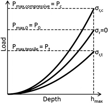
At the same time, Bolshakov et al.Reference Bolshakov, Oliver and Pharr2 conducted a finite element analysis to study the same aluminum alloy as Tsui et al.,Reference Tsui, Oliver and Pharr1 to validate their results. The study revealed that residual stresses affect the amount of indentation pile-up, whose formation is favored in the presence of compressive residual stresses, affecting the results of contact area calculated with the Oliver and Pharr methodReference Oliver and Pharr4, Reference Oliver and Pharr5 and affecting the load–displacement curve. Figure 1 reproduces the idea of Bolshakov et al.Reference Bolshakov, Oliver and Pharr2 regarding the effect of residual stresses on instrumented indentation load–displacement curve. To obtain the same maximum penetration depth, materials with compressive residual stresses ( ) require a larger applied load than unstressed materials or materials with tensile residual stresses (
 ).
Effects of residual stress on instrumented indentation load curves. For the same maximum penetration depth materials with compressive residual stress (σc,t ) must have a larger load applied by the indenter than unstressed materials or with tensile residual stress, based on Ref. 2.

Recently, Mady et al.Reference Mady, Rodriguez, Gomez and Souza6 extended the results of Tsui et al.Reference Tsui, Oliver and Pharr1 and Bolshakov et al.Reference Bolshakov, Oliver and Pharr2 for a wider range of residual stress values (−5 to 2 GPa) and different levels of work hardening of the indented material. The trends described in the literatureReference Tsui, Oliver and Pharr1, Reference Bolshakov, Oliver and Pharr2 were reproduced only for low values of work hardening exponent (n), which indeed indicated that residual stresses do not affect real contact area and real hardness, but the area calculated based on the Oliver and Pharr method,Reference Oliver and Pharr4, Reference Oliver and Pharr5 due to an increase in the tendency for pile-up formation. Mady et al.Reference Mady, Rodriguez, Gomez and Souza6 also indicated that when the work hardening exponent is larger (0.3–0.5), calculated (using Oliver and Pharr method) and real (obtained from the finite element model) contact areas tend to coincide and so does the hardness calculated from both routes.
LarssonReference Larsson7 worked with instrumented indentation data to investigate the mechanical behavior of materials with residual stress and concluded that the mechanical properties calculated for materials with tensile residual stresses are more accurate than those calculated for materials with compressive ones. The author indicates that traditional equations based on the correlation between hardness and yield stress are not sufficiently accurate to determine mechanical properties in materials with medium and high levels of compressive residual stresses. Ling et al.Reference Ling, Long, Ma and Liang8 obtained that the behavior of hardness as a function of residual stresses changed more significantly for plastic residual stress (larger than the initial yield stress) than for elastic residual stresses and indicated that the relation between residual stress and real hardness was linear.
B. Residual stress calculation from IIT data
There are different methods to estimate residual stresses based on IIT data, as recently reviewed by Jang.Reference Jang9
In the late 1990s, Suresh and GiannakopoulosReference Suresh and Giannakopoulos10 proposed a model to calculate residual stress using sharp indenters, which was based on the works of Tsui et al.Reference Tsui, Oliver and Pharr1 and Bolshakov et al.Reference Bolshakov, Oliver and Pharr2 Later, in the early 2000s, Atar et al.Reference Atar, Sarioglu, Demirler, Sabri Kayali and Cimenoglu11 suggested that one of the factors in the method by Suresh and GiannakopoulosReference Suresh and Giannakopoulos10 should be neglected. More recently, Lee and KwonReference Lee and Kwon12, Reference Lee and Kwon13 interpreted the equibiaxial residual stress as a composition of a mean stress plus a stress component along the indentation axis (deviator stress) that is directly added to the surface–normal indentation pressure. A few years before, Carlsson and LarssonReference Carlsson and Larsson14, Reference Carlsson and Larsson15 analyzed the sharp indentation behavior theoretically, numerically (to explore how equibiaxial residual stress and strain fields can be determined from the global properties), and experimentally, aiming to understand the influence of residual surface stress and strain fields on global indentation parameters such as hardness and contact area. Finally, Wang et al.Reference Wang, Ozaki, Ishikawa, Nakano and Ogiso16 proposed a method for conical indenters that compares the energy (work done by the indenter) of load–displacement curves of stressed and unstressed materials. In this case,Reference Wang, Ozaki, Ishikawa, Nakano and Ogiso16 the value of residual stress was extracted from the difference between these two energy values. Other methods are available in the literature, such as that from Zhao et al.,Reference Zhao, Chen, Yan and Karlsson17 which was selected to determine uniaxial residual stress and mechanical properties in bond coat and multilayer systems; and that from Lee et al.,Reference Lee, Lee, Hyun and Kim18 who proposed a method based on dimensional analysis to estimate equi- and nonequibiaxial residual stresses. Many of the methods above will be described in more detail in Sec. II.
Taljat and PharrReference Taljat, Pharr, Vinic, Kraft, Moody and Shaffer19 considered whether residual stresses could be better measured with spherical indenters, which lead Swadener et al.Reference Swadener, Taljat and Pharr20 to propose a method to calculate residual stresses based on spherical indentation. These authorsReference Swadener, Taljat and Pharr20 described two different methods: one of them requires previous knowledge of the yield stress of the material and is based on the idea that the penetration depth to induce yielding is affected by residual stresses. The second method is based on a correlation between mean contact pressure and normalized contact radius (ratio between the radius of contact area and indenter radius), which can be directly obtained from analyses of load–displacement data.Reference Swadener, Taljat and Pharr20 Lepienski et al.Reference Lepienski, Pharr, Park, Watkins, Misra and Zhang21 analyzed if indentation methods to calculate residual stresses could be applied to thin films but encountered difficulties due to film surface roughness, substrate effects, and problems in producing an appropriate reference specimen for comparison.
In this work, a set of finite element analysis was conducted to simulate the conical indentation of a system with a hard film onto a softer substrate. Different values of film work hardening exponent, film yield strength, film elastic modulus, film Poisson’s ratio, and film residual stress were considered to cover values often seen for Physical Vapor Deposition films. The load–displacement curves obtained from the simulations were then used to calculate the film residual stresses based on the models of Suresh and Giannakopoulos,Reference Suresh and Giannakopoulos10 Lee and Kwon,Reference Lee and Kwon12, Reference Lee and Kwon13 and Wang et al.Reference Wang, Ozaki, Ishikawa, Nakano and Ogiso16 Additionally, residual stress were calculated based on the modification that Atar et al.Reference Atar, Sarioglu, Demirler, Sabri Kayali and Cimenoglu11 suggested to the Suresh and Giannakopoulos methodReference Suresh and Giannakopoulos10 and two routes not published previously. The calculated values were then plotted against the ones used as an input in the finite element model to analyze the correlation.
II. EXISTING MODELS
A. Suresh and Giannakopoulos method
Suresh and GiannakopoulosReference Suresh and Giannakopoulos10 proposed a method to calculate residual stresses, according to which an equibiaxial stress state would be equivalent to a hydrostatic stress state plus an uniaxial stress component. In this case, the sign would depend on the nature of residual stress (compressive or tensile). The authors deduced equations for both tensile and compressive residual stresses and considered indentations with both limited maximum penetration depth or limited maximum load. In this work, only the maximum penetration depth analyses will be considered.
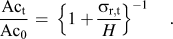
To deduce the equation to calculate residual stresses, the authorsReference Suresh and Giannakopoulos10 followed a sequence of steps in which a material with tensile residual stresses would be initially indented to a load (P t) and a penetration depth (h max), as indicated in Fig. 1. Keeping the maximum penetration depth constant, these authors considered that the material undergo a hypothetical relaxation of residual stress. In this case, the change in the stress state of the material would result in a hydrostatic stress (that cancels the preexisting one) plus a compressive normal stress with the magnitude of the residual stresses. Based on this concept, authors deduced Eq. (1) and, from that, Eq. (2), where Act is the contact area of the material with tensile residual stress, Ac0 is the contact area of the unstressed material,  is the tensile residual stress, P 0 is the load of the unstressed material at h max, P t is the load of the material with tensile residual stress at h max, and H is the hardness of the material (mean average pressure), which was considered independent of residual stress.

The same procedure was conducted for materials with compressive residual stress loaded to the same penetration depth, which provided Eqs. (3) and (4). However, as indicated in these equations, a factor f = sin (θ), where θ is the complement of the indenter angle α (θ = 22° for Vickers indenter and 24.7° for Berkovich), was included in the analyses of compressive residual stresses. In this case,  corresponds to a force normal to the indenter surface that facilitates the contact between indenter and specimen surface.Reference Suresh and Giannakopoulos10

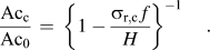
Based on experimental results, Atar et al.Reference Atar, Sarioglu, Demirler, Sabri Kayali and Cimenoglu11 suggested that f should be neglected (i.e., f = 1) in Eq. (4), providing, according to the authors, better correlation of the calculated values of residual stress with those obtained based on x-ray diffraction data.
B. Lee and Kwon method
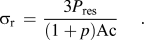
Lee and KwonReference Lee and Kwon12, Reference Lee and Kwon13 proposed a method to calculate residual stresses based on Eq. (5). In this equation, P res is the contribution of the indentation force caused by residual stress, i.e., the difference of applied loads proposed by Suresh and Giannakopoulos. However, instead of the factor f in Eqs. (3) and (4), the authors considered a correction factor of  , as indicated in Eq. (5). In this method, p is the stress ratio (p = σy,r/σx,r) and equals to one (p = 1) in the presence of equibiaxial residual stresses. Choi et al.Reference Choi, Lee, Kim, Kim and Kwon22 obtained good correlation between the residual stress values calculated based on x-ray diffraction data and those calculated with the Lee and KwonReference Lee and Kwon12, Reference Lee and Kwon13 method.
Similar to Suresh and Giannakopoulos,Reference Suresh and Giannakopoulos10 Lee and KwonReference Lee and Kwon12, Reference Lee and Kwon13 considered recoveries in indentation load and contact morphology by stress relaxation, but they also considered a reversible process. For instance, a gradual relaxation of tensile residual stresses causes a rebounding force that pushes the indenter out of the surface, explaining the increase of load and area that occur in P–h curve. Eq. (6) indicates the continuous stress relaxation for a material with tensile residual stress, in which the term P res is the rebounding force.Reference Lee and Kwon13

To use the Lee and KwonReference Lee and Kwon12, Reference Lee and Kwon13 method, it is necessary to integrate Eq. (6) according to the indenter characteristics. Thus, the contact area and residual stress must be written as a function of applied load. Lee and KwonReference Lee and Kwon12, Reference Lee and Kwon13 assumed that the residual stress relaxation varies linearly as a function of applied load, providing Eq. (5) for tensile and compressive residual stresses. The sign of the stress comes directly from P res, which is  for tensile residual stresses and
 for compressive ones. The contact area is Acc or Act for compressive or tensile residual stresses, respectively.
C. Energy method or Wang method
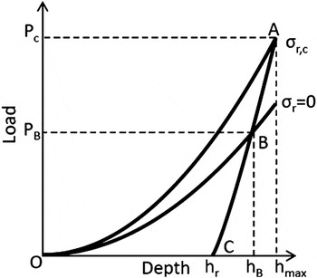
In another method, also called the energy method, Wang et al.Reference Wang, Ozaki, Ishikawa, Nakano and Ogiso16 compared the energy of a load–displacement curve of a material with compressive residual stresses with that of a stress-free material, as indicated in Fig. 2. Point B is the intersection of the unloading curve of the material with compressive residual stress and the loading curve of the unstressed material. The same idea can be used for materials with tensile residual stress, but, in this case, it is necessary to compare the loading curve of the material with tensile residual stress with the unloading curve of an unstressed material.
Comparison of a P-h curve of a material with compressive residual stress with a loading curve of an unstressed material based on Ref. 6.

Using a conical indenter, Wang et al.Reference Wang, Ozaki, Ishikawa, Nakano and Ogiso16 wrote Kick’s law for elastic–plastic loading and elastic unloading as in Eq. (7), where h r is the residual penetration depth and C and K are coefficients related to residual stress, to material properties, and to indenter geometry.Reference Mady, Rodriguez, Gomez and Souza6, Reference Wang, Ozaki, Ishikawa, Nakano and Ogiso16, Reference Rodríguez Pulecio, Moré Farias and Souza23 Note that the authors considered the same exponent for both the loading and unloading portion of the indentation load–displacement curve ( ).

The plastic work done by the indenter is obtained from the area below the loading curve and above the unloading curve. In Fig. 2, for the specimens with compressive residual stress, the work done by the indenter corresponds to area OAC. Thus, the work done by the indenter may be calculated as in Eq. (8).Reference Wang, Ozaki, Ishikawa, Nakano and Ogiso16

If the difference between the loading curve of an unstressed material and the load–displacement curve of the material with compressive residual stress (Fig. 2) is only due to the difference in residual stress, it can be stated that area OAC minus area OBC would correspond to the work done by the indenter due to the existence of residual stresses. This difference is presented in Eq. (9), where P B is the force at which the loading curve of unstressed material crosses the unloading curve of the material with compressive residual stress.Reference Wang, Ozaki, Ishikawa, Nakano and Ogiso16

For conical indenters, and assuming an equibiaxial stress state, the energy contribution of residual stresses can be approximately calculated as indicated in Eq. (10).Reference Wang, Ozaki, Ishikawa, Nakano and Ogiso16

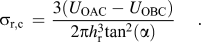
Imposing that Eqs. (9) and (10) must be equal, Eq. (11) can be used to calculate residual stresses, where A r is the residual projected area.

III. MODIFICATION ON PREEXISTING MODEL AND NEW APPROACH
A. Modification on the Wang method
In this work, the Wang et al.Reference Wang, Ozaki, Ishikawa, Nakano and Ogiso16 method was modified to adapt Kick’s law for any type of indenter [Eq. (7)]. Thus, exponents λ and m were not necessarily equal to 2. In this case, the plastic work done by the indenter, on a specimen with compressive residual stress, Eq. (8), becomes Eq. (12). Index c refers to the coefficients of the curve of the specimen with compressive residual stress.

The point of intersection of the loading curve of a material without residual stress and the unloading curve of a material with compressive residual stress (point B on Fig. 2) is found considering that the fitted equations of respective curves are equal and solving for h B. Thus, the energy of the unstressed material can be evaluated from Eq. (13). In this equation, index 0 refers to the coefficients of the curve of the unstressed specimen.

Then, during the indentation with conical indenters, residual stresses can be evaluated according to the modified Wang method as indicated in Eq. (14).
B. Approach based on the difference in hardness
Many studiesReference Tsui, Oliver and Pharr1, Reference Bolshakov, Oliver and Pharr2, Reference Suresh and Giannakopoulos10 are based on the fact that, during indentation, the average contact pressure (equivalent to hardness) is independent of residual stress. However, to be valid, this analysis requires the use of the actual contact area. A different conclusion is reached if, e.g., this type of analysis is based on the area calculated via the Oliver and Pharr method. In fact, some authors, such as Sines and Carlson,Reference Sines and Carlson3 tried to correlate residual stress and hardness values obtained from traditional tests. Following the same ideas, Ling et al.Reference Ling, Long, Ma and Liang8 observed a linear relation between hardness and residual stress and LaFontaine et al.Reference LaFontaine, Paszkiet, Korhonen and Li24 presented a linear equation to correlate hardness and residual stress. The new approach presented in this work attempts to calculate residual stresses based on the apparent difference in hardness values of stressed and unstressed samples. The idea is to take into account the linear relationship between hardness values and residual stress reported previously.Reference Sines and Carlson3, Reference Ling, Long, Ma and Liang8, Reference LaFontaine, Paszkiet, Korhonen and Li24 In this case, residual stresses are calculated based on Eq. (15), which considers not only the variation in load but also the variation in the area calculated via the Oliver and Pharr method.Reference Oliver and Pharr4, Reference Oliver and Pharr5

IV. FINITE ELEMENT MODEL
An axisymmetric two-dimensional finite element model was developed to simulate IIT of thin ceramic films deposited onto hard steel substrates. The model used was the same as the one developed previously by Mady et al.,Reference Mady, Rodriguez, Gomez and Souza6 which considers the indenter as a sharp rigid cone with half angle of 70.3° and film thickness t of 1.5 μm. The model consisted of a mesh of 16,380 elements, in which the indenter was only allowed to move in the vertical direction and the sample had symmetry conditions along the vertical axis and restriction to move vertically at the base.
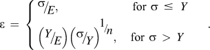
For simplicity, the constitutive model in Eq. (16) was applied to define the elastic–plastic behavior of the film and the substrate, despite the fact that more accurate descriptions may be adopted to describe the behavior of a ceramic film. The film was modeled with elastic modulus (E) of 250, 350, or 450 GPa and work hardening exponent (n) from 0.1–0.5. The Poisson’s (ν) coefficient of the film was set to 0.2 or 0.3 and the film yield strength (Y) to 4 GPa, which gives Y/E ratios on the order of 0.01. Different levels of film residual stresses ( ) were considered, varying from 2 GPa (tensile) to −4 GPa (compressive). A particular set of simulations was conducted considering Y = 8 GPa, in which n was equal to 0.3 and applied residual stress varied from 2 to −8 GPa. The substrate was modeled with elastic modulus of 200 GPa, Poisson’s coefficient of 0.29 and yield strength of 1.5 GPa. In the simulations, to vary the contribution of the substrate in the mechanical response of the system, the indenter penetration depth was limited to 0.15 μm (10% of film thickness), or 0,09 μm (6% of film thickness), or 0.06 μm (4% of film thickness).
V. RESULTS AND DISCUSSION
Using the P–h indentation curves obtained from simulation and the contact areas calculated using the Oliver and PharrReference Oliver and Pharr4, Reference Oliver and Pharr5 method, the residual stresses of the film were calculated based on the literature methods presented before, on the modification proposed to the Wang et al.Reference Wang, Ozaki, Ishikawa, Nakano and Ogiso16 method and on the method based on the difference in the calculated value of hardness.
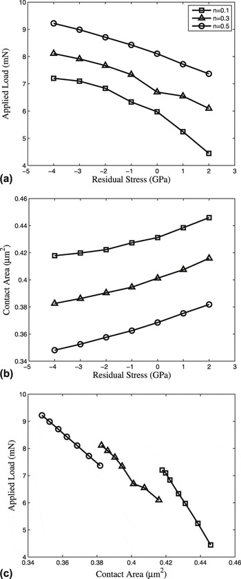
Before the application of the Lee and KwonReference Lee and Kwon12, Reference Lee and Kwon13 method, it is necessary to verify part of the conditions assumed in this case. To obtain Eq. (5), it was necessary to assume that the stress relaxation varied linearly as a function of the applied load. With this assumption, both stress and contact area are obtained as a function of applied load. Assuming that the hydrostatic stress relaxation would have the same effect as varying only the residual stress from one IIT test to another, Fig. 3 indicates that the stress relaxation is an almost linear function of applied load [Fig. 3(a)], the contact area is an almost linear function of the residual stress [Fig. 3(b)], and, therefore, the contact area can be considered a linear function of applied load [Fig. 3(c)], for a constant h max. Figure 3(c) also indicates that the slope of the curve of the applied load and contact area is a function of the film mechanical properties. Once this assumption was verified, Eq. (5) can be used to calculate the residual stress for the analyzed conditions.
Linear approximation of: (a) applied load as function of residual stress; (b) contact area as function of residual stress; (c) applied load as a function of contact area. For these sets of mechanical properties: E = 350GPa, ν=0.2, Y = 4GPa and n = 0.1, 0.3 and 0.5.

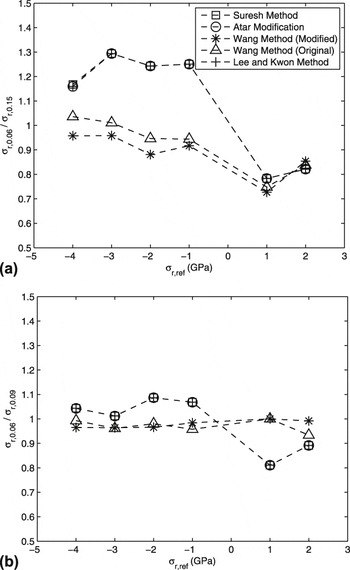
Figure 4 presents the results regarding the effect of the substrate in the overall response of the system. Figure 4(a) presents a comparison between data obtained at maximum penetration depth of 4% of film thickness and 10% of film thickness. Figure 4(b) compares results obtained with 6% and 4% of film thickness. Since values with 4% and 6% are similar, i.e., the ratio is close to one, it is possible to conclude that the substrate effect was not significant when maximum penetration depth was kept at 4% of film thickness. Results have also shown that the method by Wang et al. provided values closer to one than those obtained with the other methods, indicating that this method is less sensitive to the effect of the substrate. This result may be explained based on the fact that the effect of the substrate is more significant on the load achieved in the load–displacement curve than on the area below the curve, which is the basis of the Wang et al. method.
Ratio of the calculated residual at: (a) 4% of film thickness and (b) 6% of film thickness with the calculated residual stress at 10% of film thickness. For the given methods; and for E = 350GPa, ν = 0.2, Y = 4GPa and n = 0.3.

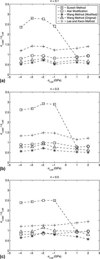
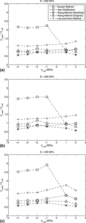
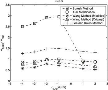
Results in Figs. 5–7 present the ratio of calculated residual stress and the value imposed in the model, considering different combinations of mechanical properties and assuming maximum penetration depths of 4% of film thickness (0.06 μm). In these figures, σr,ref is the reference value and σr,calc is the calculated value of residual stress.
Ratio of calculated residual stress and reference values of residual stress for the methods presented for: E=350GPa, ν=0.2, Y=4GPa, and (a) n = 0.1; (b) n = 0.3 and (c) n = 0.5.

Ratio of calculated residual stress and reference values of residual stress for the methods presented for: ν=0.2, Y=4GPa, n = 0.3, and (a) E=250GPa; (b) E=350GPa and (c) E=450GPa.

Ratio of calculated residual stress and reference values of residual stress for the methods presented for E=350GPa, ν=0.3, Y=4GPa and n = 0.3.

A comparison of the methods previously available in the literature, including the modification on the method by Wang et al.,Reference Wang, Ozaki, Ishikawa, Nakano and Ogiso16 indicates that in all the cases in Figs. 5–7, the procedure proposed by Suresh and GiannakopoulosReference Suresh and Giannakopoulos10 overestimated the residual stress values when they were compressive. This method provided values up to three times larger than the values imposed in the model. This difference may be related to the existence of the correction factor f, since the use of the modification proposed by Atar et al.Reference Atar, Sarioglu, Demirler, Sabri Kayali and Cimenoglu11 decreased the difference between calculated and imposed results. In Figs. 5–7, the modification proposed by Atar et al.Reference Atar, Sarioglu, Demirler, Sabri Kayali and Cimenoglu11 underestimated residual stresses when the stress was compressive. For tensile residual stress, the ratio with reference values was closer to 1.
For the Lee and Kwon method,Reference Lee and Kwon12, Reference Lee and Kwon13 results indicate an overestimation of residual stress (tensile and compressive) for the conditions in Figs. 5–7 (in these cases, the ratio was close to 1 only for large values of compressive residual stress). This result is possibly explained due to the existence of the 1.5 correction factor in residual stresses calculation, as indicated in Eq. (5).
Results obtained using the original Wang et al. methodReference Wang, Ozaki, Ishikawa, Nakano and Ogiso16 indicate that the ratio of calculated and reference provided results close to unity in Figs. 5(b) and 5(c) and Figs. 6(a) and 6(b); in the others figures, there was an underestimation of residual stress results. The modified Wang et al. method underestimated the value of residual stress in almost all cases. This result was not expected since the fitted curves were described more accurately, using general Kick’s law for loading and unloading.
Figures 5–7 indicate that the trends associated with most of the methods are approximately parallel, which can be explained by the equations in each case. The equations corresponding to the Suresh and Giannakopoulos,Reference Suresh and Giannakopoulos10 Atar et al.,Reference Atar, Sarioglu, Demirler, Sabri Kayali and Cimenoglu11 and Lee and KownReference Lee and Kwon12, Reference Lee and Kwon13 methods are essentially based on a difference of applied load divided by area. The only difference in these cases is a factor, i.e., the correction factor 1/f in the Suresh and GiannakopoulosReference Suresh and Giannakopoulos10 method, 1 in the Atar et al.Reference Atar, Sarioglu, Demirler, Sabri Kayali and Cimenoglu11 modification, and 3/(1 + p) in the Lee and KownReference Lee and Kwon12, Reference Lee and Kwon13 method [Eqs. (1), (3), and (5)]. In the last case, p was 1 for the conditions analyzed in this work, making the factor equal to 1.5.
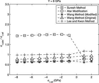
Results in Fig. 8 were obtained by increasing both the values of film yield stress and maximum imposed compressive stress to 8 GPa. In this case, the similarity observed in the majority of the results in Figs. 5–7 became more evident for a larger range of compressive residual stress, and again, original Wang et al.Reference Wang, Ozaki, Ishikawa, Nakano and Ogiso16 and Lee and KwonReference Lee and Kwon12, Reference Lee and Kwon13 had the best correlation with the imposed values of compressive residual stresses. In this case, the Lee and KwonReference Lee and Kwon12, Reference Lee and Kwon13 method gave the best result for tensile and compressive residual stresses (ratio close to one).
Ratio of calculated residual stress and reference values of residual stress for the methods presented for E=350GPa, ν=0.2, Y=8GPa and n = 0.3.

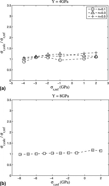
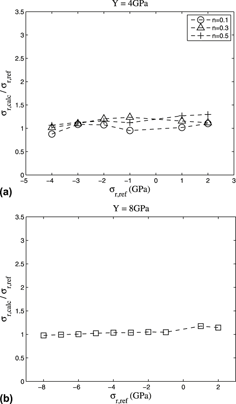
Results in Fig. 9 were obtained based on Eq. (15). This figure indicates that, both when Y = 4 GPa [Fig. 9(a)] and Y = 8 GPa [Fig. 9(b)], the error between the values of  and the imposed values of compressive stress did not exceed 20%. The correlation in the case of tensile residual stresses was worse in both cases, but the error remained lower than 20% for Y = 8 GPa [Fig. 9].
Ratio of calculated residual stress and reference values of residual stress for the new approach presented for: E=350GPa, ν=0.2, n=0.3 (a) Y=4GPa and (b) Y=8GPa.

The variable in the P–h curve that is most affected by residual stress is the applied load (the difference between stressed and unstressed materials can achieve up to 20%). The variation of other parameters, such as stiffness (S) and unloading exponent (m), remain below 3%. Thus, good results may be obtained with the methods available previously, which are based on this difference in load. However, Fig. 9 seems to indicate that accuracy in residual stress evaluation can be improved if not only the variation in load is considered but also the variation in the area calculated using the Oliver and Pharr method is included.
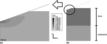
One final point to mention in the analyses conducted in this work refers to the possibility of substrate plastic deformation. In this case, Fig. 10 presents the calculated distribution of the equivalent plastic strain for the film/substrate system, where it is possible to conclude that the substrate response during the test is completely elastic. The results in Fig. 10 refer to h max of 10% of film thickness, which allows concluding that the substrate plastic deformation is also negligible for the lower penetration depths.
Distribution of equivalent plastic strain during the indentation of a system with (a) detail of contact region; (b) overall view of test.

It is important to mention that, despite the relatively good correlation of calculated and imposed values provided by some of the methods analyzed in this work, in all cases, it was still necessary to compare the stressed sample with a reference (unstressed) one. Therefore, in the application of the methods, it would be necessary to have indentation data of a sample without residual stress and all the other specimens must have the same mechanical properties as the unstressed sample. Specimens with different levels of residual stress and the same mechanical properties are not easily obtained in some cases, e.g., for physical vapor depositions (PVDs) as-deposited thin films, as indicated in Ref. Reference Mady, Rodriguez, Gomez and Souza6. This difficulty could limit the range of application of the methods, as indicated by Ref. Reference Lepienski, Pharr, Park, Watkins, Misra and Zhang21.
VI. CONCLUSIONS
In this work, a numerical analysis of instrumented indentation test on thin film-coated specimens was performed as an attempt to use test data to estimate residual stress. For the range of conditions analyzed in the finite element simulations, stiffer film (elastic modulus from 250 to 450 GPa) onto a more compliant substrate (elastic modulus of 200 GPa), it was possible to conclude that:
(i) The substrate effect was not significant when maximum penetration depth was kept at 4% of film thickness and the method provided by Wang et al. provided values less dependent of the penetration depth.
(ii) The Suresh and GiannakopoulosReference Suresh and Giannakopoulos10 method overestimated the value of compressive residual stresses, but, as suggested by Atar et al.,Reference Atar, Sarioglu, Demirler, Sabri Kayali and Cimenoglu11 the suppression of factor f improved the correlation with the input values;
(iii) The Lee and Kwon methodReference Lee and Kwon12, Reference Lee and Kwon13 provided good correlation with the imposed values for some ranges of mechanical properties; although the original Wang et al. methodReference Wang, Ozaki, Ishikawa, Nakano and Ogiso16 assumed that both the loading and unloading exponents in Kick’s law were equal to 2, this method provided the best correlation with the input values among the methods previously available in the literature. In general, the modified Wang et al. method underestimated the residual stress values.
(iv) The method based on the difference in hardness (calculated from the Oliver and Pharr method) of a specimen with and without residual stress provided good correlation with the input values.
(v) One limitation of all methods is the necessity of having a reference unstressed sample with the same mechanical properties as the tested one.
ACKNOWLEDGMENTS
The authors acknowledge FAPESP (São Paulo Research Foundation) for Grant No. 2007/04731-9 and CNPq (National Council of Technological and Scientific Development) for Grants 303780/2008-8, 150966/2009-1, and 141259/2007-8.