2.1. Governing equations and numerical schemes

All of the simulations in this paper use the filtered dimensionless compressible Navier–Stokes equations, given by

where ${\it\rho}$ is the density, $u_{i}$ is the velocity component in the $i$ th direction and $T$ is the temperature. Simulations are run non-dimensionally, with these variables non-dimensionalized by the freestream quantities. Here $p$ is the pressure, non-dimensionalized by the freestream density and velocity squared. Here $M$ is the freestream Mach number, $\mathit{Re}$ is the Reynolds number based on freestream velocity and inflow displacement thickness. Here $P_{r}$ is the Prandtl number, and is taken as 0.72 here. The coordinates $(x,y,z)$ are used in place of $(x_{1},x_{2},x_{3})$ , denoting the streamwise, bottom wall-normal and spanwise directions, respectively. The non-dimensional length scale based on the displacement thickness of the incoming boundary layer is used in the simulations. However, to avoid confusion between various boundary-layer thicknesses defined in the paper, a dimensional length is used in presenting the results based on a typical wind tunnel configuration, as discussed in § 2.3. An overbar is used for a spatially filtered variable, while a tilde denotes a Favre (density weighted) average.

The non-dimensional total energy and the resolved viscous shear stress are given respectively as

and

with the dynamic viscosity ${\it\mu}$ obtained from Sutherland’s law

where ${\it\mu}_{ref}$ is the viscosity at the reference temperature (taken here as the inflow freestream temperature), and the Sutherland constant is set as $T_{s}=110.4$  K. The dimensionless state equation for compressible flow is

The subgrid-scale (SGS) stress tensor is modelled via the classical eddy-viscosity approach as

where ${\it\nu}_{t}$ is the SGS eddy viscosity. $\widetilde{\unicode[STIX]{x1D61A}_{ij}^{\ast }}$ is the deviatoric part of the strain-rate tensor of the filtered velocity field, given by

The subgrid eddy viscosity is calculated using the mixed time scale (MTS) model of Inagaki, Kondoh & Nagano (Reference Inagaki, Kondoh and Nagano2005),

This model was developed based on a dimensionally consistent physical argument relating the asymptotic behaviour of the eddy viscosity approaching from both the wall and the potential flow. Here $T_{s}$ is a time scale, that considers contributions from both large and small eddies, given by

where $k_{s}$ is the estimated SGS turbulent energy, calculated by $k_{s}=(\widetilde{u}_{i}-\widetilde{\widetilde{u}}_{i})^{2}$ with $\widetilde{\widetilde{u}}_{i}=\overline{\overline{{\it\rho}}\,\widetilde{u}_{i}}/\overline{\overline{{\it\rho}}}$ . The constants $C_{MTS}$ and $C_{T}$ used in this paper are set to be 0.03 and 10, respectively, according to previous studies for wall-bounded compressible flow (Touber & Sandham Reference Touber and Sandham2009). The SGS heat flux ${\it\Theta}_{j}$ is modelled as

with the SGS turbulent Prandtl number fixed as $P_{r_{t}}=1$ .

A simple top-hat filter with characteristic width equal to the local grid spacing is used in deriving the governing equations, whereas an explicit filter with a width of two times the grid spacing is used as the test filter in the SGS model. No filter is applied in the wall-normal direction, where the grid is designed to provide a fine resolution. For the current 3D SWBLI cases with sidewalls, the flow field is actually filtered twice, for the side and bottom walls separately, and a special blending scheme is employed in the corner. The same blending function will also be used in the digital filter routine for turbulent inflow generation, details of which are given in § 2.2 below. The grid spacings in the $y$ and $z$ directions are designed to be very close in the vicinity of the corner, so that the filtered parameters can blend smoothly.

The governing equations are solved using a fourth-order central difference scheme for the spatial derivatives and a low-storage third-order explicit Runge–Kutta scheme to integrate in time. The code makes use of the entropy splitting of the Euler terms and the Laplacian formulation of the viscous terms to improve the stability of the non-dissipative central scheme (Sandham, Li & Yee Reference Sandham, Li and Yee2002). In addition, a variant of the standard total variation diminishing scheme is used for shock capturing (Yee, Sandham & Djomehri Reference Yee, Sandham and Djomehri1999), which is turned off within boundary layers by incorporating an additional Ducros sensor (Ducros et al. Reference Ducros, Ferrand, Nicoud, Weber, Darracq, Gacherieu and Poinsot1999).

2.2. Turbulent inflow generation

Specifying proper time-dependent turbulent inflow boundary conditions is very important for time-accurate turbulence simulations. The rescaling/recycling technique proposed by Lund (Reference Lund1998) has been widely used in previous studies on turbulent boundary layers and SWBLIs. However, this method has some drawbacks, such as pressure drift and possible low-frequency oscillation related to the recycling nature of the method. Considering the existence of secondary vortex flow in the corner between the sidewall and the bottom wall in the current study, the effect of rescaling/recycling is hard to evaluate. To avoid the high computational cost of natural or bypass transition to turbulence, the digital filter method, which has been designed to match the first- and second-order statistical moments and spectra, is employed in the present study.

The digital filter inflow generation of Xie & Castro (Reference Xie and Castro2008) is used for both the side and bottom walls. A detailed description of the optimized digital filter used here can be found in Touber (Reference Touber2010, pp. 36–43). The digital filter is robust to the choice of length scale, as long as the prescribed length scales are at least as large as the integral length scales of the real flow and sufficient downstream distance is provided to allow for the turbulence to develop (Touber & Sandham Reference Touber and Sandham2009). In the present study, the streamwise characteristic length scales $l_{x}$ for the three velocity components $u$ , $v$ and $w$ are set to $0.65{\it\delta}_{i}$ , $0.35{\it\delta}_{i}$ and $0.35{\it\delta}_{i}$ (where ${\it\delta}_{i}$ notes the 99 % boundary-layer thickness at the inflow) respectively; in the spanwise direction, the filter length scales are given by the number of filter grid points $N_{Fz}$ ( $=2l_{z}/{\rm\Delta}z$ , where $l_{z}$ is the spanwise length scale and ${\rm\Delta}z$ is the grid spacing in the $z$ direction), which are set to 20, 20 and 30 for the three velocity components respectively; similarly, in the wall-normal direction the filter grid point numbers ( $N_{Fy}=2l_{y}/{\rm\Delta}y$ ) are given as 30, 35 and 20. The same approach is applied to the sidewalls with $y$ and $z$ interchanged. Mean and root-mean-square (RMS) profiles are created beforehand for the side and bottom wall boundary layers separately. A simple blending scheme based on the streamwise momentum is used to make a smooth transition between the side and bottom boundary layers in the corner region. The mean velocity is calculated using

with

For the fluctuations, a random field is first generated and then filtered for the bottom wall and sidewalls respectively. The two filtered random fields are then combined in the same way as for the mean field, to create a random field with appropriate length scales for both boundary layers on $y{-}z$ planes at each streamwise location. To specify the integral length scale in the streamwise direction, the newly computed random field is correlated with the previous one following the formula suggested by Xie & Castro (Reference Xie and Castro2008). The new random field is then modulated with the required RMS values. Hence, a time-dependent random field is obtained that contains a specified integral length scale in the streamwise direction with a smooth variation near the corner.

2.3. Case set-up

In the present study, a reflected SWBLI with a moderate separation is investigated, taking sidewall effects into consideration. The inflow parameters (shown in table 1) are set in accordance with the $M=2.7$ experiments of Wang et al. (Reference Wang, Liu, Zhao, Fan and Wang2012). A full-span shock generator with angle $9^{\circ }$ is used to generate a steady incident shock with a shock angle of $28.9^{\circ }$ and a pressure ratio of 1.82, which is expected to trigger a moderate separation on a flat plate turbulent boundary layer. The bottom wall 99 % boundary-layer thickness ( ${\it\delta}$ ), which is used as the target boundary-layer thickness ( ${\it\delta}_{t}$ ) at the inviscid shock impingement point for all simulations in this paper, is estimated to be 6.9 mm, with the compressible (including density variations) boundary-layer displacement and momentum thicknesses ${\it\delta}^{\ast }=2.30~\text{mm}$ , ${\it\theta}=0.495~\text{mm}$ and Reynolds numbers $\mathit{Re}_{{\it\delta}^{\ast }}=19\,980$ , $\mathit{Re}_{{\it\theta}}=4300$ .

Table 1.

Flow conditions for the simulations, including the dimensional boundary-layer (BL) thicknesses and Reynolds number at the inflow.

To enable a comprehensive analysis of the 3D flow structures induced by the sidewalls, a set of cases were run with different widths ( $W$ ), while the height of the shock generator ( $H$ ) was kept fixed. The aspect ratio ( $\def\AR{A\mkern-8muR}\AR =W/H$ ) is 1, 2 and 4 for cases WH1, WH2 and WH4, respectively. Although there have been some studies concerning the sidewall effect on SWBLI (Bruce et al. Reference Bruce, Burton, Titchener and Babinsky2011; Burton & Babinsky Reference Burton and Babinsky2012; Eagle Reference Eagle2012; Babinsky et al. Reference Babinsky, Oorebeek and Cottingham2013), no information about the sidewall boundary condition upstream of the interaction has been provided. It could be assumed that the sidewall boundary layer is the same as the bottom wall. However, we should note that the sidewall boundary layer usually has developed along the nozzle wall before the wind tunnel test section. In particular, for experiments conducted on a flat plate insert in the main flow, the sidewall boundary layer is likely to be thicker than on the test plate. This is expected to influence the corner flow features in 3D SWBLI, and to take its potential effects into account different sidewall conditions are also considered here. A case named WH1-TS is designed to have a sidewall boundary thickness 1.4 times that of the bottom wall, based on measured data in the $M=2.7$ facility used by Wang et al. (Reference Wang, Liu, Zhao, Fan and Wang2012).

As mentioned in the introduction, the flow field induced by a fin/boundary-layer interaction has a quasi-conical structure about a virtual conical origin, which means that the sidewall flow pattern due to the interaction of the shock generator and the sidewall boundary layers depends on the position of the shock generator. More importantly, the rapid reduction of the streamwise velocity and the local Mach number inside the sidewall boundary layer distorts and weakens the main shock until it completely disappears close to the sidewall. This makes it impossible to model the sidewall effects using the infinite far-field inviscid shock jump conditions, as usually used in 2D and quasi-2D simulations, and the shock generator needs to be included. Compared with the traditional quasi-2D simulations, potential issues include the geometry-induced grid non-orthogonality and the possible influence of the expansion wave emitted from the trailing edge of the shock generator. To take these effects into account, a quasi-2D case (named baseline) with the same geometry (albeit with a smaller spanwise domain length) but no sidewall is conducted first with the same grid spacing as the above 3D cases. Considering the complexity of the flow near the corner, an additional case (named fin-slip) is run, in which the bottom wall is replaced with a slip boundary condition. This will help to clarify the role of the bottom-wall boundary-layer separation on the corner flow.

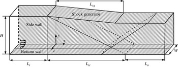
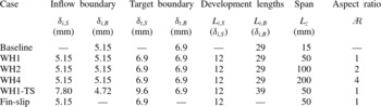
A full list of the cases conducted in the present study is given in table 2 and a sketch of the computational domain is shown in figure 1. A subscript $S$ denotes the boundary layer on the sidewall, while $B$ denotes the bottom wall. The inlet boundary-layer thicknesses are given by ${\it\delta}_{i,S}$ and ${\it\delta}_{i,B}$ , and the target boundary-layer thicknesses (defined at the inviscid shock impingement point) by ${\it\delta}_{t,S}$ and ${\it\delta}_{t,B}$ . The computational domain width is given by $L_{z}$ ( $=W$ ) and aspect ratio is defined by $\AR =L_{z}/H$ . The distance from the inflow to the shock generator is $L_{i}$ , while the distance between the shock generator leading edge and the inviscid shock impingement point is denoted as $L_{ic}$ . For all of the cases, the bottom-wall boundary-layer parameters in the interaction region are fixed as in table 2. This is achieved by adjusting the inlet boundary-layer thickness, which will be discussed in the following section.

Figure 1.

Sketch of the domain used for the simulations.

Table 2.

Details of the boundary-layer thickness and its development distance.

2.4. Domain and grid distribution

The shock generator is located on the top boundary of the domain, with the height of the shock generator leading edge $H$ set to be 50 mm, which is large enough ( $H/{\it\delta}_{t,B}=7.25$ ) to allow a quasi-conical flow field to fully develop on the sidewalls. The shock generator is set at an angle of $9^{\circ }$ to the incoming flow, which generates an oblique shock with an angle of ${\it\beta}=28.9^{\circ }$ . The leading edge of the shock generator is fixed at $x=0~\text{mm}$ , and the inviscid shock impingement point on the bottom wall is at $x=L_{ic}=90.6~\text{mm}$ downstream. The length of the shock generator in the oblique SWBLI cases is set to $L_{sg}=65~\text{mm}$ , to have an area contraction of approximately 0.2 for the supersonic channel to ensure the start of the wind tunnel in future experimental studies. This shock generator length is expected to be long enough to avoid a detrimental influence of the expansion wave (emitted from its trailing edge) on the interaction region. In the idealized case fin-slip, the shock generator was made longer to help to further reduce the expansion wave influence. A distance of $L_{o}=55~\text{mm}$ between the outlet and inviscid impingement point is set, allowing for a partial recovery of the turbulent boundary layer after reattachment.

Although the use of a digital filter to generate the inflow boundary condition significantly reduces the length required for boundary-layer development, there should nevertheless be enough distance to allow the boundary layers to adjust to an equilibrium state before the interaction (Xie & Castro Reference Xie and Castro2008; Touber & Sandham Reference Touber and Sandham2009). The fin/boundary-layer interaction on the sidewall occurs much earlier compared with the main interaction near the bottom wall. Thus, we need to ensure that the sidewall development distance $L_{i,S}$ (equal to $L_{i}$ ) is long enough, even though the development distance for the bottom wall boundary layer $L_{i,B}$ (equal to $L_{i}+L_{ic}$ ) will be longer than strictly necessary, which increases the domain length required compared with the quasi-2D case.

The development of the boundary layer generated by the digital filter was assessed by a set of quasi-2D simulations to make sure that the boundary layer reaches the target state over a development length of $L_{i}+L_{ic}$ . It was found that a distance of 12 times the inflow boundary-layer thickness is enough to obtain realistic turbulent mean and RMS profiles from the digital filter inflow generator used. Accordingly, the initial length is set to be $L_{i}=12{\it\delta}_{i,S}$ . For the cases WH1, WH2 and WH4, in which the sidewall boundary-layer thickness is the same as the bottom wall ( ${\it\delta}_{t,S}={\it\delta}_{t,B}=6.9~\text{mm}$ ), test runs confirmed that an incoming boundary layer with ${\it\delta}_{i}=5.15~\text{mm}$ will develop to the target boundary thickness (with an error of 0.5 %) at the impingement position. For the case WH1-TS (with ${\it\delta}_{t,S}=9.6~\text{mm}$ and ${\it\delta}_{t,B}=6.9~\text{mm}$ ), in which the increase of sidewall boundary-layer development length $L_{i}$ increases the development length for the bottom boundary layer ( $L_{i}+L_{ic}$ ), the inflow boundary-layer thickness on the bottom wall needed to be reduced to obtain the target boundary thickness. It is found the inflow profile with ${\it\delta}_{i,S}=7.8~\text{mm}$ and ${\it\delta}_{i,B}=4.72~\text{mm}$ resulted in errors below 1.0 % for the target boundary layers.

The present 3D simulations require fine grids near the two sidewalls and the bottom wall. This means the grid needs to be refined in both directions in the cross-flow plane close to the walls. This increases greatly the mesh size required for a structured grid. A stretched grid is used near the wall in both the $y$ and $z$ directions, which changes gradually to a uniform grid in the core flow with the required spacing. Grid smoothness is important, especially when high-order schemes are used. Two grid stretching functions with at least second-order continuity at the interface are combined to give coordinates $y_{i}$ in the direction normal to the bottom wall as

where $y_{mid}$ is the middle of the domain, while the parameters $a$ , $b$ and $c$ are fixed by continuity considerations up to second order. A predefined distance from the wall, $y_{b}$ , is used to specify the region for grid stretching, with $N_{yb}$ used to set the number of grid points to be placed inside this region. The fifth-order polynomial enables the grid to change quickly from a highly stretched grid near the wall to an almost uniform grid away from the wall. For the present study, the same function is used to generate a stretched grid in the direction normal to the sidewalls. For each case, three parameters were used to adjust the grid density: $y_{b}$ , $N_{yb}$ and ${\it\beta}_{y}$ . 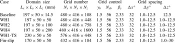Details about the grid control parameters and the resulting grid spacing are given in table 3. The streamwise direction has a uniform grid distribution, with ${\rm\Delta}x^{+}=32$ based on the inflow turbulent boundary layer. In the $y$ direction, the grid spacing is $y_{1}^{+}=1.0$ for the first point off the wall and ${\rm\Delta}y_{max}^{+}=12.5$ in the centre of the domain. In the spanwise direction, the grid spacing is also fixed as ${\rm\Delta}z_{1}^{+}=1.0$ and ${\rm\Delta}z_{max}^{+}=12.5$ . Compared with a typical grid for quasi-2D simulations, the grid stretching near the wall is very similar, but the grid is much finer away from the wall. The total number of grid points increases from 90 million in case WH1 to approximately 320 million in case WH4.

Table 3.

Grid numbers and stretching control parameters for different cases.

Cases were also run for a half-span set-up with a symmetry condition, but yielded unphysical results near the symmetry plane. This is due to the fact that the symmetry condition enforces a zero spanwise velocity and zero spanwise gradients in the unsteady 3D turbulent field, leading to artificial turbulent structures around the symmetry plane, which finally impacts on the statistics. Hence, it was necessary to include both sidewalls in the simulations. No-slip boundary conditions were enforced on the bottom wall, two sidewalls and the region representing the shock generator on the top of the domain (figure 1). The wall temperature is fixed equal to the stagnation temperature of the inflow. The integrated characteristic scheme (Sandhu & Sandham Reference Sandhu and Sandham1994) is used for the outflow and for the top boundary upstream and downstream of the shock generator.

3.1. Inflow parameters and grid independence study

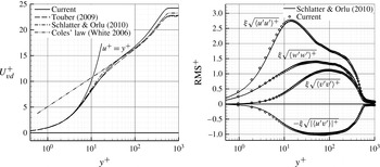
Turbulent boundary-layer mean profiles and distributions of RMS values downstream of the inlet are first evaluated. The mean inflow profile was generated using the same approach as in Touber & Sandham (Reference Touber and Sandham2009). For the inlet RMS values, the DNS results of Schlatter & Orlu (Reference Schlatter and Orlu2010) for a similar Reynolds number are used. A compressible scaling, validated by Duan, Beekman & Martin (Reference Duan, Beekman and Martin2011) for high Mach numbers, was used to transform the incompressible RMS values into compressible ones. Profiles approximately $15{\it\delta}_{i}$ downstream are compared with Coles’ law (White Reference White2006, pp. 421–424) and other reference data in figure 2. It should be noted that the Reynolds number based on the freestream flow properties and the momentum thickness, i.e.  $\mathit{Re}_{{\it\theta}}={\it\rho}_{e}U_{e}{\it\theta}_{e}/{\it\mu}_{w}$ , is approximately 4300, as given in § 2. However, the corresponding Reynolds number under the van Driest scaling, i.e.  $\mathit{Re}_{{\it\theta}_{,vd}}={\it\rho}_{w}U_{e}^{vd}{\it\theta}^{vd}/{\it\mu}_{w}$ , is approximately 1490, which is very close to the Reynolds number at 1410 in the incompressible case of Schlatter & Orlu (Reference Schlatter and Orlu2010). The subscripts ‘ $e$ ’ and ‘ $w$ ’ above denote the main flow and inner parameters parameter, while the superscript ‘ $vd$ ’ means the value under the van Driest transform. The corresponding values of $\mathit{Re}_{{\it\tau}}={\it\rho}_{w}u_{{\it\tau}}{\it\delta}_{99}/{\it\mu}_{w}$ are 516.6 and 492.2 for the present and reference cases respectively. The calculated non-dimensional freestream velocity is seen to be slightly higher, which is caused by an underestimation of the skin friction (with an error of approximately 7.9 % compared with Coles’ law). This implies an underestimation of the friction velocity by 3.8 %, which will consequently overestimate the non-dimensional velocity in the main field. The RMS values collapse very well with the DNS results of Schlatter & Orlu (Reference Schlatter and Orlu2010), which indicates that the digital filter inflow generation method used here is effective.

Figure 2.

Mean and RMS velocity distributions obtained $15{\it\delta}_{i}$ downstream of the inflow boundary. The van Driest transformation was applied to the mean velocity and a compressible scaling ${\it\xi}=\sqrt{{\it\rho}/{\it\rho}_{w}}$ (Duan et al. Reference Duan, Beekman and Martin2011) to the RMS curves.

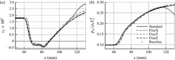
It is necessary to validate the code and the grid resolution used for the present simulations. Considering the large computing requirement for a fully 3D case with sidewalls, a grid independence study was conducted for a quasi-2D case in a rectangular computational domain ( $182\times 30\times 14.5~\text{mm}^{3}$ ) with the shock condition applied through the Rankine–Hugoniot relations. The first grid (named ‘standard’) was generated with similar resolution to the ‘baseline’ case defined in § 2.4 (see table 3), and then refined by factors of two in each of the three coordinate directions separately, referred to as FineX, FineY and FineZ in figure 3. The main difference between the cases ‘baseline’ and ‘standard’ is the use of the shock generator on the top boundary of the domain in the former, which generates an expansion wave downstream of the trailing edge of the shock generator. It can be observed that the skin friction and wall pressure distributions obtained from different grid densities are very close. The largest discrepancy is found in the FineZ case where the decrease of the skin friction is steeper before the separation, corresponding to a steeper pressure rise, and the separation length is found to be approximately 6.5 % smaller than the reference (standard) case. The refinement of the grid in the streamwise direction influences the skin friction recovery downstream. However, it makes no noticeable difference to the wall pressure distribution or the separation length. This indicates that the grid resolution used in the present study is fine enough to capture the separation region. The wall pressure decrease and skin friction rise downstream of the location $x=115~\text{mm}$ seen in the baseline case are due to this expansion wave effect. However, in the upstream flowfield, no obvious difference could be observed in the skin friction and wall pressure curves between the baseline and standard cases, with only a difference of 1.8 % in the separation length. This suggests that the expansion wave downstream of the shock generator does not have a significant influence on the separated flow region.

Figure 3.

Distributions of (a) skin friction and (b) wall pressure for different grid resolutions. The case marked Baseline includes the shock generator as the upper boundary condition whereas the other cases apply the Rankine–Hugniot jump conditions directly. The case marked standard has a similar grid resolution to the baseline case near the wall, while the other cases are for grids that are refined in each direction by a factor of two separately as indicated.

3.2. Comparison of 3D SWBLI in the centre of the domain with quasi-2D flow

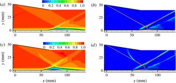
For each case, the simulation was initially run for a time of approximately $70{\it\delta}_{t,B}/U_{\infty }$ (or equivalently $2.5L_{x}/U_{\infty }$ , where $U_{\infty }$ is the freestream velocity before the interaction) to ensure that the flow field has fully developed, and then for another time period of $360{\it\delta}_{t,B}/U_{\infty }$ to obtain statistics. It covers about four times the period of the expected low-frequency component, and provides a reasonable time-averaged field, with influences of the low frequency taken into account. This enables us to have an insight into the details of the 3D flow organization, although it is not enough to conduct a spectral analysis for the low-frequency unsteadiness. Before discussing sidewall effects, we first compare the flow parameters in the central plane of the 3D cases to the quasi-2D case. In figure 4, the time- and spanwise-averaged velocity contours for the quasi-2D (baseline) and the 3D SWBLI case with $\AR =1$ (WH1) are compared, with the shock waves shown by contours of the streamwise density gradient. A limited spanwise averaging was used to improve the statistical convergence for the 3D cases, averaging over a length of $0.5{\it\delta}_{t,B}$ in the centre of the domain. Figure 4(a) shows streamwise velocity contours for the quasi-2D baseline case, which shows clearly the thickening of the boundary layer associated with the SWBLI. The time-averaged reverse flow region is between $x=67.2~\text{mm}$ (the separation point) and $x=88.3~\text{mm}$ (the reattachment point), giving a separation length of 21.1 mm. Expansion waves emitted from the trailing edge of the shock generator can be observed, which are far enough from the interaction region to have little influence on the separation length, as mentioned in the discussion of figure 3. Figure 4(b) shows contours of the streamwise density gradient ( $\partial {\it\rho}/\partial x$ ), illustrating the shock structure more clearly.

Figure 4.

Time-averaged streamwise velocity field (a,c) and streamwise density gradient (b,d) comparing the quasi-2D baseline cases (a,b) with the central plane of the 3D WH1 case in (c,d). The black line shows the time-averaged sonic line, while the pink line close to the wall shows the reverse flow region.

Unlike the uniformly distributed mean flow velocity behind the incident shock in the quasi-2D (Baseline) simulation, the central plane mean velocity in 3D-SWBLI, as shown in figure 4(c) for the case WH1, displays variations even in the core region of the flow behind the shock. A low-speed region corresponding to an interesting weak shock can be observed behind the main shock before the interaction, as seen in figure 4(c,d). The authors are not aware of published experimental observations of this phenomenon, which would have been masked by the spanwise-integration effect of traditional schlieren visualization methods. This weak shock is seen to merge with, and hence bend, the main incident shock above the interaction field. Starting from the conjunction point, the shock angle increases from $29.0^{\circ }$ to $32.4^{\circ }$ . The static pressure and density ratio across the main shock indicates that the strength of the bent main shock corresponds to a flow deflection angle of $11.5^{\circ }$ , instead of the original value of $9^{\circ }$ for the shock generator. This means the main shock is significantly strengthened through interacting with the weak shock in case WH1. Further analysis below will show that this is a distinct 3D phenomenon coming from a sidewall effect. It was detected in the central plane in both small-aspect-ratio cases WH1 and WH1-TS, but not in the large-aspect-ratio cases WH2 and WH4.

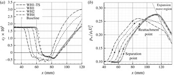
In the near-wall region, it can be seen by comparing figure 4(a,c) that the whole interaction field has moved forward under the influence of the sidewalls, with the height of the separation bubble also increased. To see the variation more clearly, distributions along the centreline of the bottom wall from cases with different aspect ratio are compared with the quasi-2D case in figure 5(a) for the skin friction and in 5(b) for the wall pressure. For the largest-aspect-ratio case WH4, there is little influence of the sidewall constraint on the centreline separation; the results correspond well to the quasi-2D case, indicating the existence of a 2D region in the centre of the domain, in accordance with the general expectation. For the other cases, the separation point (defined by the first point with $c_{f}=0$ ) has moved forward. Separation points in the two small-aspect-ratio cases WH1 and WH1-TS have moved forward by 12.5 mm ( $1.81{\it\delta}_{t,B}$ ) and 15.3 mm ( $2.21{\it\delta}_{t,B}$ ) respectively, while this distance decreases to 6.2 mm (or approximately $0.90{\it\delta}_{t,B}$ ) for case WH2 and almost zero for case WH4. Considering that the increase in sidewall boundary-layer thickness for case WH1-TS reduces the effective spanwise scale of the core flow even further compared with case WH1, it can be concluded that the smaller the aspect ratio is, the further the separation point moves forward.

Figure 5.

Comparison of (a) centreline skin friction and (b) wall pressure distributions between the 3D and quasi-2D (baseline) cases.

Apart from the separation point, the reattachment point, defined by the second crossing of $c_{f}=0$ , is also seen to be influenced. In the two small-aspect-ratio cases WH1 and WH1-TS, the reattachment points have moved forward by 5.9 mm ( $0.86{\it\delta}_{t,B}$ ) and 8.6 mm ( $1.25{\it\delta}_{t,B}$ ) respectively, while no such movement could be observed in the larger-aspect-ratio cases WH2 and WH4. This is consistent with the observations of the strength and angle changes of the incident shock in cases WH1 and WH-TS mentioned above. Geometrically, the bending of the incident shock wave moves the inviscid shock impingement point upstream by 3.4 mm ( $0.49{\it\delta}_{t,B}$ ) and 4.9 mm ( $0.71{\it\delta}_{t,B}$ ) for cases WH1 and WH-TS, respectively, which is approximately 57 % of the total movement. Additional contributions to the forward movement would come from the increase in strength of the shock and other 3D effects that will be elaborated later in the paper. The collapse of the reattachment point locations for the larger-aspect-ratio 3D cases (WH2 and WH4) suggests that the reattachment is less sensitive to the sidewall effect than the separation point, provided the aspect ratio exceeds a certain value. Based on the distance between the separation and reattachment points, the separation length can be calculated. It is interesting to find that the separation lengths in cases WH1, WH1-TS and WH2 have approximately increased to the same level, with values of 27.9, 28.1 and 28.5 mm respectively, which is approximately 30 % larger than the quasi-2D case or the largest-aspect-ratio case WH4. This indicates that the separation length alone is not sufficient to measure 3D effects, and both the separation and reattachment point locations need to be taken into account.

The wall pressure distributions on figure 5(b) exhibit the effect of the expansion wave emitted from the trailing edge of the shock generator. When the expansion wave impinges on the bottom-wall boundary layer, the local wall pressure decreases sharply, marked on the figure by the crossing point between each curve and the dotted line. It can be seen that the streamwise location of this crossing point moves downstream as the reattachment point moves upstream when the aspect ratio is decreased. This is at least partly due to the initial stages of the boundary recovery process, since the earlier the reattachment occurs, the thinner the boundary layer downstream, and the later the expansion wave will act on the boundary layer. Separation and reattachment points are also marked on the figure and there is no obvious influence of the expansion wave on the separated region. Considering that the pressure distributions downstream of the reattachment point in cases WH2 and WH4 are very close to the baseline case, it is reasonable to suppose that the expansion wave has a minor effect overall. For cases WH1 and WH1-TS, the separation field as a whole moves upstream and should be even less affected. The earlier pressure drop seen in these two cases is due to sidewall effects reaching the central plane, which will be discussed in the following sections.

4.1. Three-dimensional separation pattern

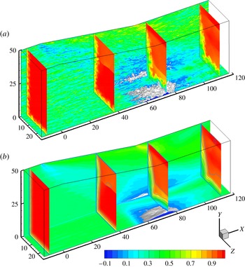
While the variations in centreline parameters show strong sidewall effects, the physical explanations for the changes can only be found by further analysis of the full 3D flowfields. Instantaneous and time-averaged velocity fields for case WH1 are presented in figure 6 in half of the domain (from the centreline to one sidewall). The near-wall low-speed streaks can be clearly seen in the instantaneous field shown in figure 6(a) on both the sidewall and the bottom wall before the interaction. Local boundary-layer thickening can be observed, both in the corner and centre of the domain. The averaged velocity field shown in figure 6(b) is highly 3D, with reverse flow regions appearing on the sidewalls near the corner and near the centreline of the domain. For the central separation, the local boundary-layer thickness and separation bubble height both increase towards the central plane. Taking into account the thickening of the boundary layer and the reverse flow region in the front part of the interaction (see figure 4), the central separation will appear curved when viewed on a plane at a certain distance away from the wall, as shown in PIV results of Dussauge et al. (Reference Dussauge, Dupont and Debieve2006), even though the wall separation may actually possess a flat front, as we shall see below.

Figure 6.

Instantaneous (a) and time-averaged (b) streamwise velocity field from case WH1, showing half the computational domain from the centreline to the sidewall. Two slices are plotted close to the side wall (at $z^{+}=10$ based on the inflow boundary layer) and the bottom wall (at $y^{+}=10$ ), together with the iso surface of $u=0$ (white) and four slices at streamwise locations $x=-10$ , 30, 72 and 110 mm.

Surface flow visualization has been proven to be an effective method to explore the 3D boundary-layer separation pattern in experiments (Reda & Murphy Reference Reda and Murphy1973; Bookey et al. Reference Bookey, Wyckham and Smits2005; Babinsky et al. Reference Babinsky, Oorebeek and Cottingham2013), with the flow separation, reattachment and other surface flow features clearly identifiable. The sidewall flow pattern is discussed first, since it is similar for the different cases simulated here. Figure 7 shows sidewall skin friction lines (with arrows) starting upstream of the incident shock and local pressure contour lines (orange), with a reverse flow region (defined as $(\partial u/\partial z)_{w}\leqslant 0$ near the corner shown with a filled contour. A 3D separation also occurs on the sidewall. Considering the sweepback effect on the sidewall (discussed in more detail later in the paper), this can be approximated by the black contour defined by the line with zero skin friction component normal to the incident shock i.e.  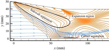$(\partial u/\partial z)_{w}\sin {\it\beta}+(\partial v/\partial z)_{w}\cos {\it\beta}=0$ , where ${\it\beta}$ is the incident shock angle. Streamlines coming from upstream and downstream converge at the separation line, but do not pass through it. To show the sidewall separation more clearly, only the skin friction lines starting upstream are plotted here. Near the bottom wall, the small corner separation is seen to be isolated from the sidewall separation. Upstream of this, a strong adverse pressure gradient is observed, which will be further discussed in § 5. The pressure distribution downstream of the interaction shows the influence of the expansion wave from the trailing edge of the shock generator.

Figure 7.

Sidewall flow pattern in case WH2, showing skin friction lines (arrows), pressure contour lines (orange), corner reverse flow region (filled contour) and sidewall separation (enclosed by the black contour).

Figure 8.

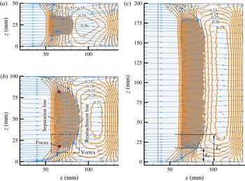
Wall separation pattern, illustrated by the reverse flow region ( $(\partial u/\partial y)_{w}\leqslant 0$ , filled contour) and skin friction lines (with arrows) for the cases with different aspect ratios: (a) WH1, (b) WH2 and (c) WH4. The local wall pressure distribution is superimposed (orange contour lines).

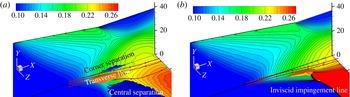
Figure 8 shows a comparison of the separation topology on the bottom wall for cases WH1, WH2 and WH4, in which the reverse flow region ( $(\partial u/\partial y)_{w}\leqslant 0$ , shown with a filled contour), skin friction lines ( $(\partial u/\partial y)_{w}/x=(\partial w/\partial y)_{w}/z$ , shown with arrows) and wall pressure contours (orange) are plotted simultaneously, to emphasize the spatial relationship between different flow features. The wall flow pattern in case WH1-TS is similar to case WH1, and is not shown here. For each case, a main reverse flow region in the centre of the channel and two tiny corner reverse flow regions close to the sidewalls are found. The central separations present similar wall flow patterns as the previous experimental studies (Reda & Murphy Reference Reda and Murphy1973; Babinsky et al. Reference Babinsky, Oorebeek and Cottingham2013). Taking the case WH2 for example (see figure 8 b), the wall streamlines and reverse flow distribution agree very well with the description of Reda & Murphy (Reference Reda and Murphy1973) with respect to the wall-flow visualization. The separation line is straight over the central part of the channel, while the reattachment line is seen to be curved, making the separation length dependent on the spanwise location and giving a larger recirculation region near the centreline. A tornado vortex is created on each side of the central separation region, with convergence of the streamlines to a focus, inducing a highly 3D velocity field there. The foci are found to be located slightly downstream of the central separation line, and close to the side edge of the central reverse flow region. A notable gap is observed between the central reverse flow and the sidewalls in all the cases, and the wall skin friction lines indicate the existence of strong transverse flow in the gap, which transports the near-wall fluid from the corner into the central reverse region, feeding the tornado vortices.

Cases WH1 and WH4 show similar wall-flow patterns as case WH2 near the sidewall, despite obvious differences in the spanwise scales. The distance measured from the edge of the central reverse field to the sidewall can be defined as the gap scale $L_{C}$ (marked on figure 8 c). It is interesting to note that the gap scale stays approximately at the same level, slightly increasing from 14.1 mm in case WH1 to 16.5 mm in case WH2 and 17.5 mm in case WH4. Compared with case WH1, the increase of sidewall boundary-layer thickness in case WH1-TS also increases the gap slightly to 16.3 mm. Consequently, the main central separation is seen to be reduced by the attached flow gap, especially for the small-aspect-ratio cases WH1 and WH1-TS. For example, the spanwise scale of the central reverse region in case WH1-TS has reduced to approximately 17.5 mm, which is only approximately 35 % of the channel width. By contrast, in the large aspect ratio case WH4, for which the gap scale is relatively small compared with the spanwise scale of the domain, a considerable length of a 2D region, identified by the reattachment line and the wall pressure distribution, could be observed. Considering that the spanwise location of the focus inside the tornado vortex is rather close to the side of the central reverse region, the value of $L_{C}$ could also be regarded as the distance of the tornado vortex away from the sidewall.

The pressure contours, illustrated by orange contour lines in figure 8, show that the surface pressure rise near the corner starts further upstream compared with the channel central region, as was also seen in the experimental results of Babinsky et al. (Reference Babinsky, Oorebeek and Cottingham2013). Despite the limited spanwise extent of the separation region, the wall pressure across the reverse flow region is relatively uniform in the spanwise direction, even in case WH1. By contrast, strong three-dimensionality is observed after the reattachment point, with the direction changes of the skin friction lines seen to follow the near-wall pressure gradients. Moreover, the existence of the tornado vortex is also seen to be related to the curving of the reattachment line and pressure contour lines. We will find some clues to these phenomena from the main shock distortion in our later discussion.

4.2. Three-dimensionality of shock waves

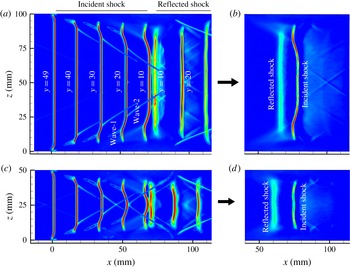
In § 3.2 it was mentioned that the incident shock is bent and strengthened by the sidewall effect in case WH1 (figure 4 c,d). To get a better view of this phenomenon, shock wave locations identified from the streamwise density gradient are investigated in the full 3D space. Figure 9(a,c) show the evolution of the shock wave structures above the interaction for cases WH2 and WH1, respectively, in which the shock structures obtained from five different $x{-}z$ planes at different heights are plotted on one graph, while figure 9(b,d) show the shock structures in the $x{-}z$ plane close to the mean shock impingement point (at $y=6~\text{mm}$ close to the top of the recirculation bubble) for which the incident shock has already passed the reflected shock. For the current simulation set-up, a plane oblique shock is generated from the leading edge of the shock generator placed at $x=0$ and $y=50~\text{mm}$ . As it propagates downstream, the main incident shock is distorted starting from its side edges, which are seen to be accompanied by a compression wave region upstream (wave-1, marked at $y=20~\text{mm}$ in figure 9) and a weak shock wave downstream (wave-2). The sidewall shock (wave-2) distorts the main shock and increases the pressure gradient across it (with more details to be presented in § 5), especially in the region where the two sidewall shocks meet. This indicates that some three-dimensionality already appears on the main incident shock before its interaction with the bottom wall boundary layer.

Figure 9.

Distortion of the main shock waves is illustrated with contours of the time-averaged streamwise density gradient for cases WH2 (a,b), and WH1 (c,d). (a,c) Show shock waves above the interaction region, with shock structures from five different $x{-}z$ planes (at $y=49$ , 40, 30, 20 and 10 mm) superimposed for both cases. (b,d) Show the shock structures on the $x{-}z$ plane at $y=6~\text{mm}$ , i.e. close to the location where the shock impinges on the apex of the recirculation bubble.

The three-dimensionality seen here is related to the sidewall boundary layer, or more accurately the swept SWBLI between the main shock and the sidewall boundary layer. It is clear that the shock wave originating from the shock generator has played two different roles in the present cases. On the bottom boundary layer it works as the incident shock for a reflected SWBLI, while on the sidewall it acts as the sweepback shock for a swept SWBLI. It should be noted that the same flow deflection angle in the reflected SWBLI usually triggers a stronger interaction considering the combined compression induced by the incident and the reflected shock. A flow deflection angle ${\it\alpha}$ in the range of interest for the reflected SWBLI induces a much weaker swept SWBLI. Most studies on reflected SWBLIs are conducted around ${\it\alpha}=10^{\circ }$ (Reda & Murphy Reference Reda and Murphy1973; Dupont et al. Reference Dupont, Haddad and Debieve2006; Ganapathisubramani et al. Reference Ganapathisubramani, Clemens and Dolling2007; Touber & Sandham Reference Touber and Sandham2009; Eagle Reference Eagle2012), since a slightly larger angle, for example ${\it\alpha}=12^{\circ }$ (Bookey et al. Reference Bookey, Wyckham and Smits2005), is enough to trigger highly unsteady large-scale separation. By contrast, for the swept SWBLI, taking the work of Alvi & Settles (Reference Alvi and Settles1992) at Mach 2.9 as an example, a flow deflection angle of ${\it\alpha}=10^{\circ }$ could only create a weak swept interaction, while the typical swept interaction field was established between ${\it\alpha}=16^{\circ }$ and $25^{\circ }$ . In the physical model for a strong swept SWBLI field (Alvi & Settles Reference Alvi and Settles1992), the compression wave (wave-1) here appears as a separation shock, which forms a typical ‘ ${\it\lambda}$ ’ shock structure together with part of the curved main shock (named as ‘rear shock’). A slip line appears, starting from the ‘triple point’ of the ‘ ${\it\lambda}$ ’ shock, and the main shock curves forward (Lu Reference Lu1993) above the ‘triple point’, with the curvature deceased as the interaction strengthens. The main features of the weak swept SWBLI field suggested by Alvi & Settles (Reference Alvi and Settles1992) can be identified in figure 9. Special attention should be paid to the curving of the main shock above the ‘triple point’, which can be attributed to the complex 3D triple shock interaction. Although not understood completely, Lu (Reference Lu1993) suggested that the curving of the main shock is due to the requirement that the pressure across the slip line must be equal, analogous to the curved ‘Mach stem’ in a 2D Mach reflection. In addition to the experimental observation, the curving of the main shock is clearly related to the weak sidewall shock (wave-2). More detailed discussion about the swept SWBLI field will be presented in § 5, where we will see that these swept-SWBLI-induced 3D features on the incident shock have a significant influence on the flow structures near the bottom wall.

It can be seen from figure 9 that both the compression wave (wave-1) and the weak shock wave (wave-2) propagate towards the centre of the domain as the main incident shock develops downstream. Different spanwise scales produce different shock wave patterns in the interaction region. For the small-aspect-ratio case WH1, the distortions due to the two sidewalls reach the central plane and pass through each other, with the whole incident shock influenced. However, for the large-aspect-ratio cases (WH2 and WH4), the distortion from the sidewalls does not reach the central plane, and part of the incident shock is still spanwise-uniform before its interaction with the bottom-wall boundary layer. Thus, bending of the main shock in the central plane was only observed in the small-aspect-ratio cases WH1 and WH1-TS. It should be noted that such a distortion on the main shock would be seen as an increasing of the shock thickness in the traditional schlieren visualization, considering the spanwise integration, and this is indeed observed in the image obtained in Dussauge & Piponniau (Reference Dussauge and Piponniau2008). However, the schlieren method could not show the weak shock (wave-2 in figure 9 a), since it occupies all of the space between the main incident shock and the shock generator when viewed from the spanwise direction, and no obvious difference on the shock-induced density gradient could be detected in the spanwise-integrated flowfield. Interestingly, although the incident shock has been obviously distorted, the time-averaged reflected shock waves seen in figure 9 are planar even for the smallest-aspect-ratio case WH1 as shown in figure 9(d), except for the thickening induced by its instantaneous spanwise wrinkling and low-frequency oscillation (Wu & Martin Reference Wu and Martin2008; Humble et al. Reference Humble, Elsinga, Scarano and van Oudheusden2009; Priebe & Martin Reference Priebe and Martin2012). This can be explained by the spanwise-uniform pressure distribution before separation (see figure 8).

4.3. Sweepback effect and confinement of core flow

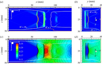
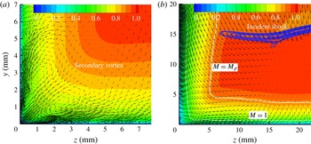
The main shock waves (both the incident and reflected ones) only exist in a limited region in the channel central area, which is especially notable for the smaller-aspect-ratio case WH1 (see figure 9 c), and a considerable distance is seen between the shock foot and the sidewall. To get an insight into this phenomenon and its potential significance, figure 10(a) shows the shock structure on a horizontal ( $x{-}z$ ) plane 14 mm above the bottom wall for case WH1, with corresponding pressure contours given in figure 10(c). Results for a vertical ( $y{-}z$ ) plane at $x=70~\text{mm}$ are shown alongside in figure 10(b,d). In general, one expects that shock waves can extend as far as the sonic line (the red line) into a boundary layer, however in these cases the shock waves stop well before the sonic line of the sidewall boundary layer. This is significant because the shock-induced streamwise pressure jump does not extend very far into the near-wall region. Instead, it is seen that the shock waves always stop at a line with a particular ‘penetration’ Mach number $M_{p}$ . An analysis presented below will show that the penetration Mach number in the current cases is $M_{p}=2.07$ . This is confirmed by the numerical results shown in figure 10, where the contour line of $M_{p}=2.07$ fits the shock foot locations on the sidewall boundary layer across the whole domain. The region where the main shock exists can be defined as the core flow. The flow becomes very complex closer to the sidewalls under a 3D pressure gradient which forces the fluid to move around the side edges of the shock as shown in figure 10(c,d).

Figure 10.

The spanwise extent of the main shock waves is shown on an $x{-}z$ plane at $y=14~\text{mm}$ (on the left in (a) and (c)) and a $y{-}z$ plane at $x=70~\text{mm}$ (on the right in (b) and (d)) for case WH1. (a,b) Show the streamwise density gradient, while plots (b) and (d) show pressure contours. The two solid lines mark the locations of $M=1.0$ (the sonic line in red) and $M_{p}=2.07$ (the penetration Mach number in white) respectively.

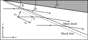
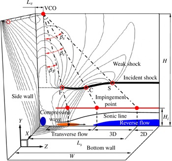
The sweepback effect of the main shock on the sidewall is found to be the reason why its foot cannot reach the sonic line. It is well known that the distorted (thickened or separated) boundary layer in swept SWBLI possesses a quasi-conical structure with a well-defined sweepback angle (Alvi & Settles Reference Alvi and Settles1992; Lu Reference Lu1993). The incoming flow velocity can therefore be decomposed into normal and tangential components with respect to the shock face (as sketched in figure 11), with the normal component responsible for the pressure jump across the shock. The main shock plane (solid line) and the trace of the shock foot (dashed line) are shown in figure 11 in an $x{-}y$ plane. The trace of the shock foot is slightly upstream, considering that the main shock face is curved approaching the wall, but the angle of the shock foot trace (denoted as ${\it\beta}_{f}$ ) is, to a good approximation, equal to the shock angle (denoted as ${\it\beta}$ ). Given that the limiting normal Mach number component is equal to the one at the shock foot location, the flow Mach number at the shock foot (or equivalently the penetration Mach number $M_{p}$ introduced above) is

Figure 11.

Sketch to illustrate important features of the swept SWBLI, including the main shock angle ${\it\beta}$ and the trace of the shock foot ${\it\beta}_{f}$ .

For the present case at a freestream Mach number of 2.7 and flow deflecting angle of $9^{\circ }$ , the main shock angle is ${\it\beta}=28.9^{\circ }$ and the corresponding penetration Mach number $M_{p}=2.07$ . As shown in figure 10, the simulations show that a line at this constant Mach number successfully captures the main shock foot. Hence, the above analysis can be used to predict the shock extent. When the incident shock approaches the bottom boundary, interaction with the sidewall shock increases the angle ${\it\beta}$ , therefore $M_{p}$ decreases correspondingly. It should be noted that the sweepback effect is only relevant to the sidewall boundary layer. At the bottom wall, the incident shock still penetrates to the sonic line as seen in figure 4.

According to the quasi-conical structure of swept SWBLI, the distance of the penetration to the sidewall would be expected to increase almost linearly as the shock propagates downstream. This means that the spanwise width of the core flow in the SWBLI field decreases linearly before reaching the interaction region on the bottom wall. Thus, it is not necessary for the incident shock to be strong enough to separate the sidewall boundary layer for flow to lose two-dimensionality, especially when the aspect ratio is small.

5.1. Extent of conical flow

The main features of the swept SWBLI above the main interaction zone, on a horizontal $x{-}z$ plane at a height of $y=20~\text{mm}$ , are shown in figure 12 for part of the spanwise flow field close to a sidewall in case WH2. The horizontal plane shown here enables us to have a direct comparison between flow patterns in the main field and the separation field near the bottom wall. 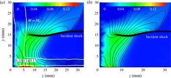A plane normal to the shock would be an alternative way to show the interaction, however the basic flow pattern captured on $x{-}z$ planes will be the same if the quasi-conical structure is valid for the interaction field. The background colour contours show the local pressure and spanwise velocity in figure 12(a,b), respectively, while compression and shock waves are shown by the white contour lines of the streamwise density gradient. In contrast to most previous studies on such an interaction, which concentrated on the shock-induced separation pattern (Alvi & Settles Reference Alvi and Settles1992; Lu Reference Lu1993), the focus here is on the distortion of the main shock.

Figure 12.

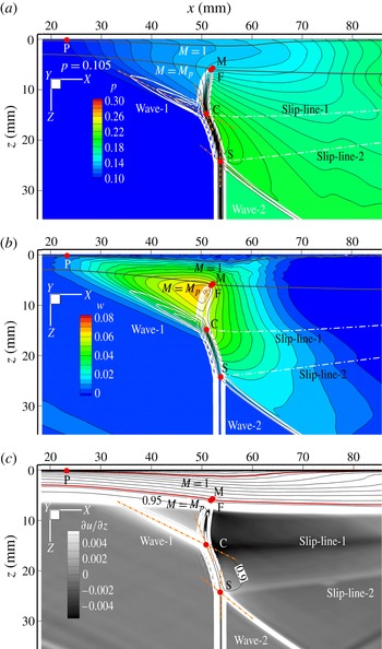
Main features of the swept SWBLI field above the interaction, captured on an $x{-}z$ plane at $y=20~\text{mm}$ in case WH2. The background contours show the local pressure (a) and the spanwise velocity (b). The shock and compression waves are shown by the white solid contour lines of the streamwise density gradient. Points are marked for some important features of the flow structure: P is the start of the pressure rise, F is the location of the shock foot, M is the projection of the shock foot on the penetration line (the line where $M=M_{p}$ ), C is the intersection point of the compression wave (wave-1) with the incident shock (also the ‘triple point’ of the ‘ ${\it\lambda}$ ’ shock in stronger swept SWBLI Lu Reference Lu1993) and S is the intersection point of the weak sidewall shock (wave-2) with the incident shock. The cuts of two 3D slip-faces are marked by the white dash-dotted lines labelled ‘slip-line-1’ and ‘slip-line-2’, based on the $\partial u/\partial z$ field shown in (c). The streamwise velocity in the zone between the two slip-faces (see the slim contour lines in (c)) is lower than in the surrounding region.

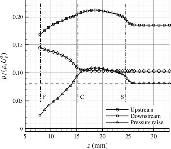
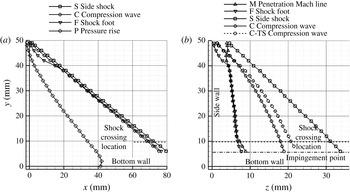
Distinct features of the main shock distortion are marked in figure 12. The shock foot location is marked as point F, located where the density gradient contour has decreased to a value of 0.01. Point M then denotes the projection of point F onto the penetration line ( $M=M_{p}$ , as defined in § 4.3). Point C marks the interaction point of the compression wave (wave-1 in figure 9) with the incident shock, which is actually the ‘triple point’ described by Lu (Reference Lu1993). Point S is the interaction point of the weak shock (wave-2 in figure 9), which is another triple point, marking the start of the main shock curvature. Point P represents the start of the pressure rise on the sidewall (approximated by the location with a 5 % pressure rise, relative to the pressure jump across the incident shock), which can be considered as the start of the swept SWBLI. The sidewall boundary layer is thickened under the effect of the adverse pressure gradient, leading to the compression wave (wave-1) and a clear region of finite spanwise velocity (directed away from the sidewall). The peak of the spanwise velocity is seen to be located close to the shock foot in figure 12(b).

In a 2D triple shock interaction field, a slip-line deriving from the triple point usually arises. Similarly, a slip-face forms in the 3D triple shock interaction here. By checking the velocity gradient $\partial u/\partial z$ , shown in figure 12(c), two 3D slip-faces are detected. Cuts through the slip-faces, arising from the triple points C and S on the plane at $y=20~\text{mm}$ , are marked in figure 12, named as ‘slip-line-1’ and ‘slip-line-2’. It should be noted that the ‘slip-line’ here is just a cut through the slip-face in 3D space and is not a true material line, which is different from the ‘slip-line’ in 2D interactions. Thus, the velocity direction on the plane is not necessarily parallel to the ‘slip-line’ here, which could also be proved by the spanwise velocity near the slip-lines in figure 12(b).

Figure 13 shows the pressure distribution across the distorted incident shock to quantify the shock strength modification. Owing to the existence of the leading compression wave, the pressure upstream of the incident shock near the sidewall is much higher than the inflow pressure in the main field, and it decreases gradually to the main flow pressure from the shock foot F to point C. By contrast, the pressure downstream is seen to increase gradually between points F and C. Remarkably, the pressure downstream of the main shock has already reached a higher level than in the main flow around point C. Consequently, the outer main shock has to be strengthened and curved at point C to match this pressure rise on the two sides of the slip-face (marked as ‘slip-line-1’ in figure 12), as supposed by Lu (Reference Lu1993). It can be seen in figure 13 that the pressure downstream of the curved main shock between points C and S is indeed at a higher level than in the main field. However, the pressure downstream of the curved shock has to be adjusted to the undisturbed part of the main shock in the region further outside, and this is achieved by the wake shock starting from the triple point S (wave-2 in figure 12), accompanied by another slip-face (marked by ‘slip-line-2’ in figure 12). A direct consequence of the above adjustment in the shock wave pattern is the modification of the pressure rise across the main shock. Between points C and S, the pressure rise increases up to 32 % higher than in the main field, while in the region from point C to F it decreases towards zero.

Figure 13.

Pressure distribution across the distorted incident shock on the $x{-}z$ plane at $y=20~\text{mm}$ , marked with the points F, C and S as defined in figure 12.

The streamwise and spanwise propagation of the points F, P, C and S along the main shock, giving the distortion of the incident shock face induced by the swept SWBLI, are shown in figure 14 for case WH2. The projections of these points on the $x{-}y$ and $y{-}z$ planes are shown in figure 14(a,b) separately. The trace of point M is not shown in figure 14(a) because it is the same as for point F on the $x{-}y$ plane. It can be seen that the quasi-conical structure is followed for most of the interaction region, except during the inception stage. The trace of the shock foot (Point F) on the $x{-}y$ plane is almost parallel to the main shock, which means that ${\it\beta}_{f}={\it\beta}$ (see figure 11 and § 4.3) is a good approximation. More interesting features are shown on the $y{-}z$ plane in figure 14(b). It can be observed that the points F and M propagate almost linearly away from the sidewall until they meet the reflected shock (at the ‘shock crossing location’ in figure 14). Before the conical flow pattern is established, the shock foot (marked by point F) penetrates into the boundary layer as far as the sonic line, so that the lines F and M are different for $y>40~\text{mm}$ . Except for this incipient region, all of the points F, C and S propagate almost linearly away from the sidewall before the main shock reaches the impingement point. Thus, the whole flow pattern can be reasonably described by a quasi-conical structure, and the straight lines originating at $(z,y)=(4.5~\text{mm},50~\text{mm})$ are reasonable fits for the traces of points F, C and S in the region $y<30~\text{mm}$ . It should be noted that the point S propagates so fast in the spanwise direction that it has passed through the middle plane at $z=25~\text{mm}$ in the cases WH1 and WH1-S, with part of the flow around the central plane compressed twice by the secondary sidewall shock coming from two opposite directions, as we saw in figure 9.

Figure 14.

Traces of key points delineating the shock structure at different downstream positions, illustrating the quasi-conical structure of the swept SWBLI in case WH2: (a) projection of the points on the $x{-}y$ plane; (b) projection of the points on the $z{-}y$ plane. An additional trace of point C from case WH1-TS (denoted ‘C-TS’) is also shown to check the influence of the sidewall boundary-layer thickness. The location where the incident shock goes through the reflected shock is marked as the ‘shock crossing location’ while the location where the shock meets the top of the separation bubble is marked as the ‘impingement point’.

For the oblique SWBLI on the bottom wall, the structure of the incident shock (i.e. the spanwise location of the marker points S, C and F) close to the shock impingement point is of particular interest. It can be seen from figure 14 that the point C ends at about $z=18.5~\text{mm}$ , which is close to the edge of the central separation in cases WH2 ( $z=16.5~\text{mm}$ ) and WH4 ( $z=17.5~\text{mm}$ ). Recalling that point C is the location where the shock strength starts to decrease, it is clear that the rapid decrease of shock strength between point C and the shock foot F explains why the central separation terminates around point C in cases WH2 and WH4. In the small-aspect-ratio case WH1 the separation extends closer to the sidewall, to about $z=14.1~\text{mm}$ . This can be attributed to the fact that the shock is strengthened by the weak shock from the opposite sidewall, since the point S has already passed through the central plane in this case. For the case WH1-TS, the increase of sidewall boundary-layer thickness has made the point C move towards the domain centre (curve C-TS in figure 14 b), stopping the central separation further from the sidewall at $z=16.3~\text{mm}$ .

Aside from the spanwise scale, the pattern of the bottom separation has also been modified by the distorted incident shock. As mentioned above, the main shock between points C and S has been curved and strengthened. A potential consequence is that the curved main shock could touch the bottom wall earlier, and the corresponding spanwise pressure gradient component makes it possible to expel low-momentum fluid near the wall towards the centre of the domain. This would then explain the forward curving of the reattachment line as we see in figure 8, which will also promote the formation of a 3D separation. For the large spanwise cases WH2 and WH4, the 2D region on the incident shock is found to coincide rather well with the 2D reverse flow region indicated by the straight reattachment lines and pressure contour lines in figure 8, both of which are located in the central region 35 mm away from the sidewall (or with $L_{S}=35~\text{mm}$ as marked in figure 8 c).

5.2. Wave reflection near the corner

To clarify the influence of the sidewall and corner flow behaviour, the corner flow fields from cases WH2 and fin-slip are analysed. In the case fin-slip, a slip-wall boundary condition replaced the original turbulent boundary layer on the bottom wall. This case can be considered as a limiting case when the bottom-wall boundary-layer thickness decreases to zero, and will be useful to separate the basic flow pattern of swept SWBLI from the complex interaction with the bottom-wall boundary layer. Pressure distributions on the sidewall and bottom wall near the corner are presented in figure 15. The central and corner separation regions in case WH2 are illustrated with an isosurface of $u=0$ (blue), while high spanwise velocity regions are shown by an isosurface (orange) at 11 % of the incoming freestream velocity, with superposed streamlines showing how the flow is deflected. High spanwise flow has already been observed for the swept SWBLI above the interactions region (figure 12 b) and here we see the influence of the wall. Comparing figure 15(a) and (b) we can see that the presence of the bottom-wall boundary layer leads to a region of high spanwise velocity that is flatter, stronger and further upstream compared with the fin-slip case with no boundary layer. No reverse flow is observed in the fin-slip case, but the same pressure rise in the corner upstream of the main interaction is observed in both cases. A similar surface pressure distribution near the corner was obtained in the experiments of Babinsky et al. (Reference Babinsky, Oorebeek and Cottingham2013), who attributed it to the corner shock (or compression wave) induced by the displacement effect of a corner separation. Since the slip-wall here acts as a symmetry plane on which the reflection of the incident shock occurs, it is natural to suppose that some features of the swept SWBLI field would reflect from the bottom wall, for example the compression wave ahead the main shock. Given a reflection process, it will not be necessary to have a displacement effect caused by a corner separation to form the pressure rise observed above. Furthermore, a reflection assumption will enable us to estimate the corner pressure rise from the pressure distribution in the swept SWBLI field.

Figure 15.

Wall pressure contours illustrating the flow behaviour near the corner. The plot includes three streamlines starting from the height $y=0.15$ , 2.15 and 4.15 mm. (a) Case WH2, superposed with surfaces showing the corner flow separation, region of high transverse flow and the central separation. (b) The same features, where they exist, for the fin-slip case.

To have a closer view of the flow behaviour near the corner, velocity vector fields in $y{-}z$ planes are investigated. Figure 16 shows two planes located (a) upstream ( $x=35~\text{mm}$ ) and (b) at the beginning ( $x=60~\text{mm}$ ) of the interaction, superimposed by the streamwise velocity contours. As expected, the dominant feature of the corner flow upstream of the interaction is the secondary streamwise vortex pair. It should be noted that the velocity vector length in figure 16(a) is eight times that used in figure 16(b) to show the vortex pair clearly, and the transverse flow is actually relatively small upstream of the interaction. When the flow reaches the interaction region, a strong global transverse flow overwhelms the original secondary vortex pair, with only a tiny vortex remaining in the corner.

Figure 16.

Corner vortex features shown with velocity vectors and streamwise velocity contours in $y{-}z$ planes for case WH2. The planes are taken: (a) upstream of the interaction field ( $x=35~\text{mm}$ ), where the secondary corner vortex pair is the dominant feature; and (b) at the beginning of the interaction on the bottom wall ( $x=60~\text{mm}$ ).

The spanwise velocity and the local pressure distribution on a $y{-}z$ plane at $x=60~\text{mm}$ are presented in figure 17(a), while their counterparts for the fin-slip case are shown in figure 17(b). The pressure contour lines in case WH2 in the $y{-}z$ plane are seen to be perpendicular to the bottom wall in the sidewall-affected region (for $0~\text{mm}<z<10~\text{mm}$ ) near the bottom wall outside the boundary layer, in accordance with the compression wave reflection model discussed above. In the adjacent region (for $10~\text{mm}<z<15~\text{mm}$ ), the pressure contour lines turn towards the centre of the domain, due to the pressure rise induced by the compression wave ahead the main central separation. Pressure contour lines in $3~\text{mm}<z<8~\text{mm}$ , which are normal to the wall above the sonic line, are also observed to deviate markedly towards the centre of the domain beneath the sonic line, while no such phenomenon is observed in the fin-slip case. It is probable that the high pressure downstream propagates upstream through the subsonic zone, causing the observed bending of the pressure contour lines.

Figure 17.

Comparison of pressure (black contour lines) and spanwise velocity (background contour colour) distributions near the corner at $x=60~\text{mm}$ for (a) case WH2 and (b) case fin-slip. A noteworthy feature is the high spanwise velocity region observed below the sonic line in case WH2.

Figure 18.

Summary schematic of the oblique SWBLI with sidewall effect. Pressure contours from the fin-slip case are used as a background together with filled contours showing key features. The incident shock created from the shock generator is distorted by the weak sidewall shock at point S and by a compression wave at point C. The shock foot (point F) is relatively far from the wall due to a sweepback effect. The incident shock is strengthened between point S and C, but weakens rapidly from point C to F, with a 3D pressure field developing near the corner. Following the quasi-conical structure of the swept SWBLI, all of these features propagate approximately linearly away from the sidewall before the shock impinges on the distorted bottom boundary layer, triggering the separation.

As we have mentioned previously, the transverse flow appearing in the attached region between the main separation and the corner is an important feature of the three-dimensionality. A particularly high spanwise velocity region (with a peak value up to 20 % the inflow freestream velocity) is observed in figure 17(a) close to the bottom wall, located beneath the sonic line. It should be noted that the compression wave discussed above has a particular sweepback angle relative to the bottom-wall boundary layer. Analogous to the action of sweepback on the sidewall boundary layer, the pressure gradient implied by the swept compression wave will further drive the low velocity flow within the bottom-wall boundary layer away from the corner, contributing to the peak of the transverse flow close to the wall. Since the streamwise velocity component is relatively small close to the wall, the velocity vector (also the direction of the streamlines in this region) will turn obviously towards the centre of the domain, as was seen in figures 8 and 14(a). A consequence will be the accumulation of low-momentum flow in the central region, which probably exacerbates the central separation, as mentioned in § 4.1. At the same time, the strong spanwise flow probably helps to alleviate the accumulation of low-momentum fluid in the corner and reduces the local boundary-layer thickness as seen in figure 6(b).

5.3. Physical model for the 3D interaction

Based on the preceding analysis of the numerical results, a physical model for the creation of the 3D separation pattern in an oblique SWBLI field under the effect of the sidewalls can now be established. Figure 18 shows the key features superimposed on contours of pressure on the side and bottom walls and on a plane located just upstream of the shock impingement. After being generated at the leading edge of the shock generator, the incident shock passes over the sidewall boundary layer, and the basic flow pattern of a weak swept SWBLI on the sidewall is gradually built up. The thickening of the sidewall boundary layer induces a secondary compression region upstream, which in stronger swept SWBLI would present as a separation shock and form a typical ‘ ${\it\lambda}$ ’ shock structure together with part of the curved main shock. The main shock above the compression wave region is found to be curved forward as a result of the 3D triple shock interaction (Lu Reference Lu1993). Further away from the sidewall, a secondary sidewall shock is formed downstream of the incident shock due to the difference in flow direction and static pressure between the sidewall influenced field and the undisturbed 2D zone (see figure 12). Thus, an obvious distortion is present on the main incident shock, accompanied by the compression wave (ending at point C) and the sidewall shock (starting from point S), and a considerable distance is observed between the shock foot (point F) and the sidewall due to the sweepback effect that causes the shock to end at the penetration Mach number (as discussed in § 4.3).

The main shock distortion and secondary waves move gradually towards the centre of the domain as the incident shock propagates towards the bottom wall, and the three-dimensionality develops as follows. (i) When the incident shock reaches the bottom wall, the first effect is the reflection of the compression wave in the corner region, which forms a corner compression wave. The transverse pressure gradient created by the compression wave drives the flow towards the centre of the domain, with a particularly strong spanwise flow under the sonic line of the bottom boundary layer. (ii) When the 3D incident shock gets closer to the bottom wall, the adverse pressure gradient triggers separation of the boundary layer. Since the shock strength denoted by the pressure rise decreases dramatically from point C to point F, the boundary layer is less likely to separate. Thus, the spanwise extent of the central separation is seen to end close to point C. (iii) The main shock between point C and S is curved forward and strengthened, and the forward curvature makes that part of the shock reach the bottom boundary layer earlier. This could help to form the curved reattachment line between the points indicated by $L_{C}$ and $L_{S}$ in figure 8(c). For the cases WH2 and WH4, the 2D part of the incident shock is found to coincide rather well with the straight part of the reattachment lines. (iv) The spanwise pressure gradient associated with the curved shock between points C and S expels the separated fluid beneath the boundary layer towards the centre of the domain. Together with the transverse flow upstream as described in step (i) above, a tornado vortex is created on each side of the central separation region (see figure 8).

It can be seen from the above discussion that, although it is relatively weak, the swept SWBLI formed on the sidewall plays an important role in the 3D separation of the main oblique SWBLI field. The bottom wall boundary layer is also important as it decides the ability of the boundary layer to resist the adverse pressure gradient, and hence determines the separation size in the centre, which will have some influence on the reflected shock and corner compression wave strength. The spanwise extension of the main separation would be expected to move from point C towards point F as the incident shock becomes stronger. Given the above physical model, even if the incident shock is not strong enough to trigger a separation, the flow can depart from the 2D solution, as was observed by Reda & Murphy (Reference Reda and Murphy1973).

Based on this physical model, we can estimate the three-dimensionality in the oblique SWBLI with sidewall effects. Figure 18 also shows the virtual conical origin point on the leading edge of the shock generator at a distance $L_{v}$ from the sidewall and three angles, ${\it\beta}_{S}$ , ${\it\beta}_{C}$ and ${\it\beta}_{F}$ , which correspond to the angles of the lines tracing the movement of points S, C and F, respectively. These parameters are determined by the swept SWBLI, and can be obtained independently of the main oblique SWBLI. For the present cases WH1, WH2 and WH4, we have $L_{v}\approx 4.5~\text{mm}$ , ${\it\beta}_{S}=33.5^{\circ }$ , ${\it\beta}_{C}=15.3^{\circ }$ and ${\it\beta}_{F}=4.5^{\circ }$ . Given the height of the interaction defined by the impingement point $H_{i}$ and height of the shock generator $H$ , the spanwise location of the point S near the interaction field can be estimated by

To have $L_{S}=W/2$ , i.e. the case in which the point S reaches the centre of the domain just as the incident shock propagates into interaction region, we need

Considering that both $L_{v}$ and $H_{i}$ are generally much smaller than $H$ , the left-hand side can be regarded as the effective aspect ratio of the domain, defined by $\AR_{e}=(W-2L_{v})/H$ , while the right-hand side is approximately $2\tan {\it\beta}_{S}$ . A similar conclusion can be obtained for points C and F, and the lengths $L_{C}$ and $L_{F}$ can be defined similarly to $L_{S}$ . According to the location of these critical points near the interaction region, we can classify oblique SWBLI with the expected 3D flow features, depending on the effective aspect ratio $\AR_{e}$ , which is close to the geometrical aspect ratio $\AR =W/H$ when the value of $L_{v}$ is much smaller than $W$ .

1. (i) For $\AR_{e}>2\tan ({\it\beta}_{S})$ , the sidewall shock wave does not propagate to the centre of the domain, and a 2D portion of the incident shock is preserved. For moderate separation cases, the reattachment point in this region is expected to be reasonably well predicted by quasi-2D simulations (this applies to cases WH2 and WH4 in the present study). The gap between the central and sidewall separations will be close to the location of point C, which can be estimated as $L_{C}=\tan ({\it\beta}_{C})(H-H_{i})+L_{v}$ . Meanwhile, the spanwise extent of the 2D reverse flow region can be estimated by the 2D extent of the incident shock, i.e.  $L_{S}=\tan ({\it\beta}_{S})(H-H_{i})+L_{v}$ , which is demonstrated by the wall flow pattern presented in figure 8(c).

2. (ii) For $2\tan ({\it\beta}_{C})< \AR_{e}<2\tan ({\it\beta}_{S})$ , we have $L_{C}<W/2<L_{S}$ . In this case, the sidewall shock waves have crossed in the centre of the domain, while the compression waves have not yet reached the central plane (this applies to cases WH1 and WH1-TS in the present study). Thus, the whole incident shock is distorted and the whole separation field is highly 3D. Distortion and strengthening of the incident shock is observed in the central plane of the domain (see figure 5), and the attachment point moves significantly further forward compared with corresponding quasi-2D cases. For lower values of $\AR_{e}$ in this range the gap between the central separation and the sidewall moves from point C towards point F, located between $\tan ({\it\beta}_{F})(H-H_{i})+L_{v}$ and $\tan ({\it\beta}_{C})(H-H_{i})+L_{v}$ .

3. (iii) For the case $2\tan ({\it\beta}_{F})< \AR_{e}<2\tan ({\it\beta}_{C})$ , the sidewall compression wave also passes through the centre of the domain, and the entire incident shock is significantly weakened. The more gradual pressure rise means that the separation is reduced in both the streamwise and spanwise directions and might even disappear. In addition, the sidewall flows start to interact, with a potential consequence being additional unsteadiness of the flow.

4. (iv) For very small aspect ratio when $\AR_{e}<2\tan ({\it\beta}_{F})$ , the channel is fully occupied by the sidewall turbulent boundary layers before the interaction, and we should not expect to see the same type of SWBLI on the bottom wall.