Introduction

Sea-ice cover in polar regions plays an important role in the heat budget of the atmosphere through the reflection of solar radiation and the insulation of the atmosphere from the ocean. Our interest in the variation of sea-ice extent in the Arctic Ocean and its peripheral seas is rapidly growing: the Arctic has been found to have a great influence on the climatic change in mid-latitudes of the Northern Hemisphere through atmospheric teleconnections such as the North Atlantic Oscillation (NAO; Reference Wallace and GutzlerWallace and Gutzler, 1981) and the Arctic Oscillation (Reference Thompson and WallaceThompson and Wallace, 1998). Since the advent of satellite-borne microwave radiometers in the 1970s, great progress has been made in terms of spatial distribution, seasonal and interannual variabilities, regional variability and decadal trend. For example, Reference Parkinson, Cavalieri, Gloersen, Zwally and ComisoParkinson and others (1999) showed seasonal, regional and interannual variabilities in the Arctic sea-ice extents over the years 1978–96, and indicated that the interannual variability differs considerably from region to region. They also found that the Northern Hemisphere sea-ice extent is decreasing with an overall trend of –2.8% per decade, which agrees well with previous studies by Reference Johannessen, Miles and BjørgoJohannessen and others (1995), Reference Bjørgo, Johannessen and MilesBjørgo and others (1997) and Reference Cavalieri, Gloersen, Parkinson, Comiso and ZwallyCavalieri and others (1997).

As for the mechanism of sea-ice growth and decay, Reference Shuchman, Josberger, Russel, Fischer, Johannessen and GloersenShuchman and others (1998) studied intra-annual and interannual variabilities of the Greenland Sea Odden sea ice in relation to meteorological conditions and concluded that the key meteorological parameters responsible for ice formation and decay are, in order of importance, air temperature, wind speed and wind direction. On the other hand, Reference Kimura and WakatsuchiKimura and Wakatsuchi (1999, Reference Kimura and Wakatsuchi2001) insisted that the advance and retreat of sea ice in the Arctic marginal seas are controlled by sea-ice drifts by winds, on the basis of good correlations between sea-ice extents and geostrophic winds. Possible cause-and-effect relations between sea-ice growth and atmospheric circulation have also been discussed by Reference Parkinson and GratzParkinson and Gratz (1983), Reference Cavalieri and ParkinsonCavalieri and Parkinson (1987), Reference ParkinsonParkinson (1990), Reference AgnewAgnew (1993) and Reference Parkinson, Cavalieri, Gloersen, Zwally and ComisoParkinson and others (1999) with special reference to possible roles of the air-pressure system.

Nevertheless, our knowledge of the role of atmospheric circulation in the growth/decay of sea-ice extent is still fragmentary and controversial. Moreover, regional differences of interannual variability of sea-ice extent remain to be explained. The objective of this paper is therefore to examine the relation between sea-ice cover and atmospheric circulation for all the Arctic marginal seas in an attempt to give answers to these questions. For this purpose, we compare monthly means of objectively re-analyzed meteorological observations with sea-ice growth rates during a month, instead of monthly means of sea-ice extent. The controlling factor for sea-ice growth and decay in the Arctic marginal seas is also briefly discussed.

Data and Method of Analysis

In 1996, the US National Snow and Ice Data Center (NSIDC) released Northern Hemisphere EASE-Grid Weekly Snow Cover and Sea Ice Extent Version 2 on a CD-ROM (Reference Armstrong and BrodzikArmstrong and Brodzik, 2002a). The dataset contains weekly sea-ice extents observed with the Scanning Multichannel Microwave Radiometer on board the Nimbus 7 satellite and the Special Sensor Microwave/Imager on board the Defense Meteorological Satellite Program’s satellites. Sea-ice cover is identified as such on an equal-area grid (25 km × 25 km) when the ice concentration is >15%. The dataset analyzed here covers the period October 1978-August 1995. The missing data for the 2 weeks 28 December 1987 to 10 January 1988 are interpolated by duplicating the data for the week 11-17 January 1988, and missing data for the other 8weeks are neglected in this analysis. The effect of this interpolation on the results is assumed to be minimal.

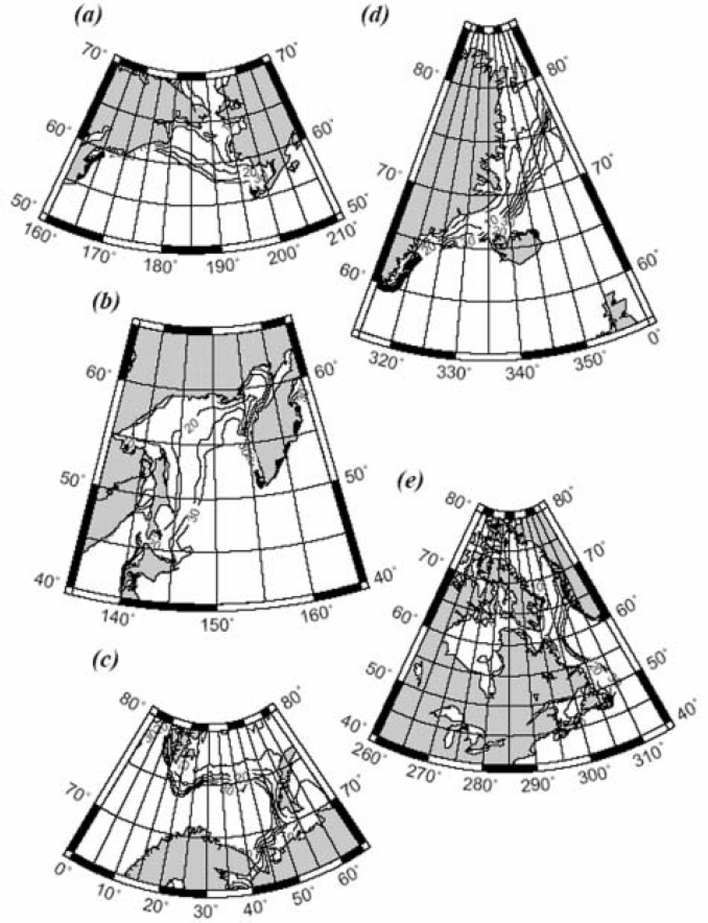
We examine the role of atmospheric circulation in the interannual variation of sea ice with reference to five marginal seas around the Arctic Ocean: the Barents Sea (65-80˚ N, 0-65˚ E), the Greenland Sea (55-85˚ N, 0–45˚ W), the Labrador Sea (40-80˚ N, 45-100˚ W), the Bering Sea (50–70˚N, 160˚E–150˚W) and the Sea of Okhotsk (40– 65˚ N, 135–165˚ E). Geographical maps of the five marginal seas are shown in Figure 1. Note that the Labrador Sea is defined as including Baffin Bay, Hudson Bay and the Gulf of St Lawrence, and the Sea of Okhotsk as including the Sea of Japan. In Figure 1, the 17year mean distribution of the ice-edge zone (with an ice concentration of 0.15) is shown as a function of week number starting from the first week of September.

Fig. 1.

Geographical maps of the five marginal seas around the Arctic Ocean and mean seasonal advances of ice-edge zone (defined as with ice concentration of 0.15) averaged over the 17 years 1979–95. The five marginal seas are: (a) Bering Sea; (b) Sea of Okhotsk; (c) Barents Sea; (d) Greenland Sea; and (e) Labrador Sea. Numerals indicate week numbers, beginning from the first week of September, at 5 week intervals. For example, 10, 20, 30 corresponds roughly to early November, mid-January and late March, respectively.

For each marginal sea, 3 monthly means of ice extent have been calculated for the winter (defined as January– March), spring (April–June), summer (July–September) and autumn (October–December). Since the sea-ice extent is maximal in winter, we are concerned with wintertime ice extents when we discuss interannual variation of sea-ice cover. On the other hand, the growth rate of sea ice is generally maximal during the late autumn–early winter, and we use monthly means of ice extent during November– January when we discuss sea-ice growth in relation to atmospheric circulation.

Generally the scale of atmospheric circulation responsible for ice growth may be equal to or less than a few hundred kilometers. To examine the role of atmospheric circulation in sea-ice growth, therefore, we should look at a region with a scale of less than a few hundred kilometers rather than a whole regional sea. After inspecting regional characteristics of seasonal changes of sea-ice cover, we selected the following sub-regions as representative of the five marginal seas: the Barents Sea sub-region (74–78˚ N, 28–54˚ E), the Greenland Sea sub-region (69–74˚N, 14–20˚ W), the Labrador Sea sub-region (56–63˚ N, 56–61˚ W), the Bering Sea sub-region (58–63˚N, 168˚ E–173˚W) and the Okhotsk Sea sub-region (50–56˚ N, 144–148˚ E). Geographical locations of the subregions are represented by trapeziums in Figures 3–9.

As for atmospheric data, we use monthly means of the objectively analyzed sea-level pressures (SLPs) and 850 hPa air temperatures (T850) for the years 1978–95, compiled by the US National Centers for Environmental Prediction/US National Center for Atmospheric Research (NCEP/NCAR) and distributed by the American Meteorological Society (Reference KistlerKistler and others, 2001). The SLP fields provide information on the atmospheric pressure system and surface geostrophic wind, while the T850 fields provide information on the air temperature of the lower troposphere.

Thus far, many authors have compared sea-ice extents with contemporary air-pressure patterns in order to discuss how sea-ice extent is related to atmospheric circulation (e.g. Reference Parkinson and GratzParkinson and Gratz, 1983; Reference Cavalieri and ParkinsonCavalieri and Parkinson, 1987; Reference ParkinsonParkinson, 1990; Reference AgnewAgnew, 1993). However, monthly means of sea-ice extent in winter are subjected not only to mean circulations over a month but also to those over the preceding months. That is to say, a monthly mean of atmospheric circulation is only responsible for sea-ice growth during the month. In this paper, therefore, we use a monthly growth rate of sea-ice extent defined by (sea-ice extent for the last week of a month – sea-ice extent for the first week of the month)/(total area of the region concerned). Note that the last (or first) week of a month is defined as the week in which the last (or first) day of the month is included. The growth rate thus defined usually represents the growth rate of sea-ice extent during 4 weeks but occasionally that during 5weeks. To normalize the monthly growth rate, growth rates calculated from ice-extent differences during 5weeks are multiplied by 4/5.

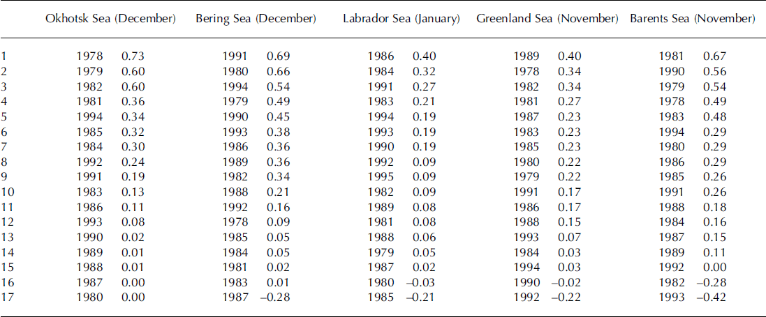
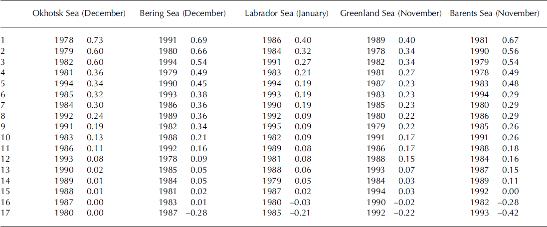
Monthly growth rates are calculated for months of rapid ice growth (November–January) during the period October 1978–August 1995. Naturally, the month of maximum growth rate depends on sub-region and varies from year to year. Growth rates for each sub-region for a selected month are shown in Table 1 in order of magnitude. The 17 growth rates are then grouped into three categories of ‘high growth rate’ (the highest six growth rates), ‘moderate growth rate’ (the middle five growth rates) and ‘low growth rate’ (the six lowest growth rates). The highest three and lowest three growth rates are additionally grouped into the categories ‘maximum growth rate’ and ‘minimum growth rate’, respectively. (Note that the groups of low and minimum growth rates sometimes include negative values.)

Table 1.

Monthly growth rates of sea-ice extent for the five Arctic marginal sea sub-regions for a selected month. The 17 growth rates are arranged in order of magnitude. The highest three growth rates are grouped into a ‘maximum growth rate’, and the lowest three into a ‘minimum growth rate’, category

Finally, composite maps of the SLP and T850 fields are prepared for these groups in order to examine the role of atmospheric circulation in the growth of sea-ice extent in the marginal seas around the Arctic Ocean.

Regional Correlations of Sea-Ice Extent in Winter

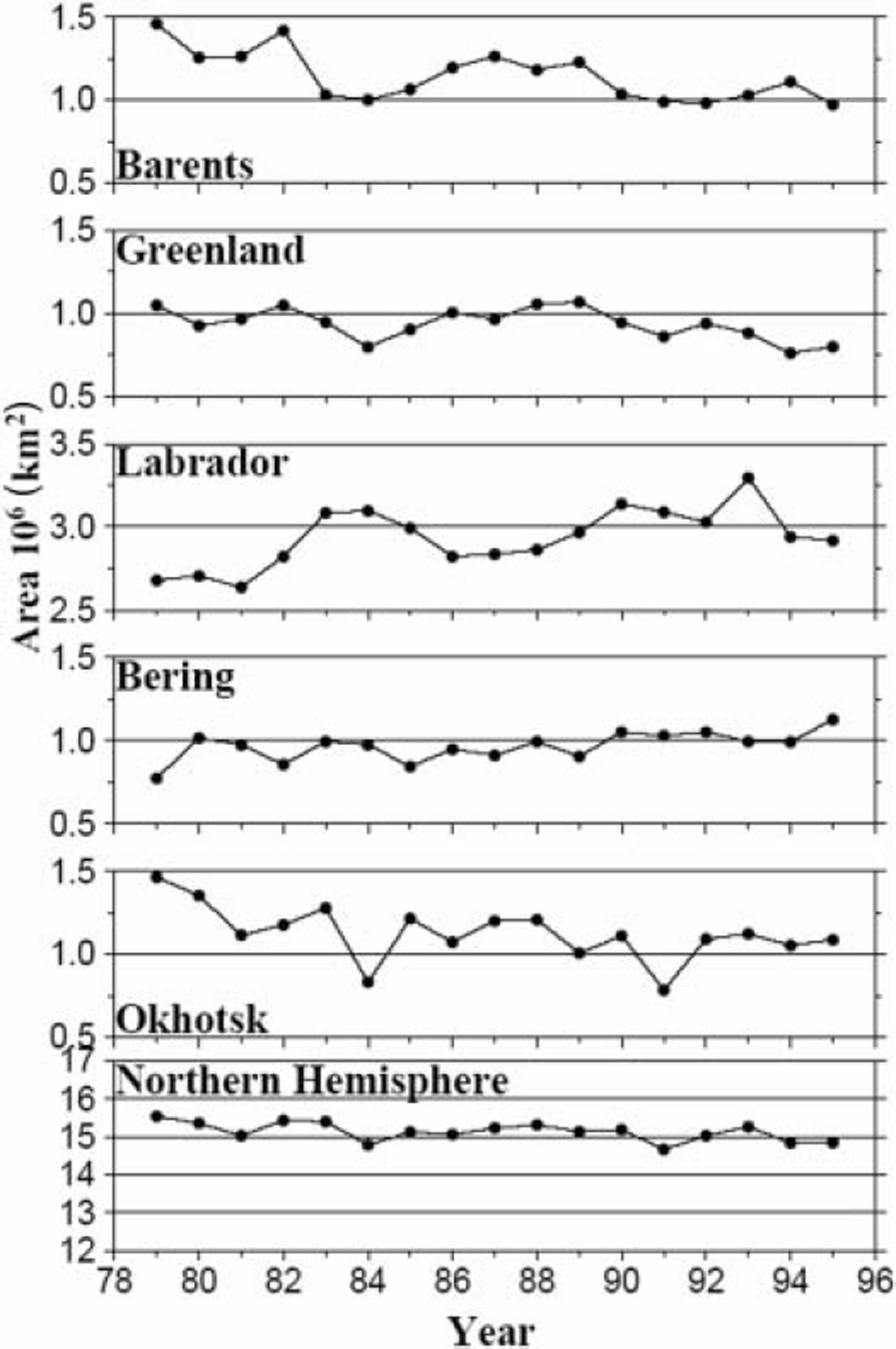
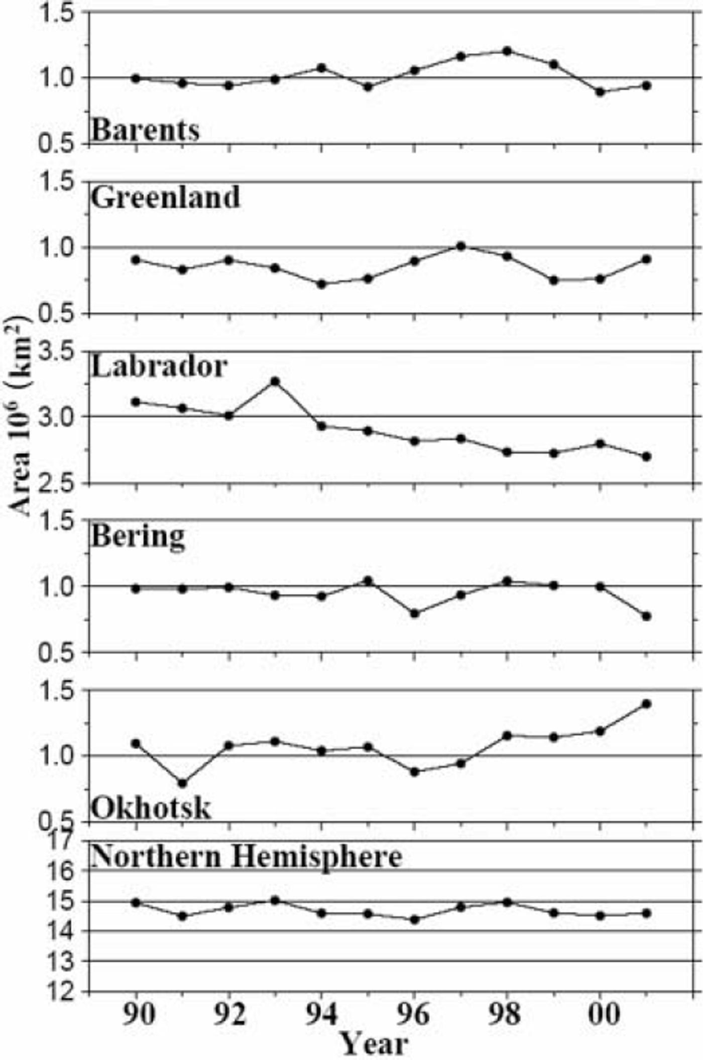
In the 17 year mean distributions of ice-edge zone in the growth season (Fig. 1), we see that sea-ice cover generally advances from north to south and/or from land to ocean. In the ice-decay season, on the other hand, sea ice retreats in the reverse order (Reference Parkinson, Comiso, Zwally, Cavalieri, Gloersen and CampbellParkinson and others, 1987; Reference Gloersen, Campbell, Cavalieri, Comiso, Parkinson and ZwallyGloersen and others, 1992). This implies that the ice-cover season is longer, and the sea-ice thickness larger, in inshore than in offshore regions. Of course, the seasonal change of sea-ice extent varies from year to year. In Figure 2, interannual variations of the 3 monthly (January-March) mean sea-ice extent are shown for the five marginal seas and the entire Northern Hemisphere. It is seen that the total area of sea-ice extent in the Northern Hemisphere has decreased by about 0.6 × 106km2 (∼4%) during the 17years. Seasonally, it has decreased more significantly in the summer and spring than in the autumn and winter, though the values are not presented here. These conclusions are generally in good agreement with those of previous studies by Reference Johannessen, Miles and BjørgoJohannessen and others (1995), Reference Bjørgo, Johannessen and MilesBjørgo and others (1997), Reference Cavalieri, Gloersen, Parkinson, Comiso and ZwallyCavalieri and others (1997) and Reference Parkinson, Cavalieri, Gloersen, Zwally and ComisoParkinson and others (1999) who used ice-extent data covering the years 1978-96. Regionally, on the other hand, the sea-ice extents of the Barents, Greenland and Okhotsk Seas are generally decreasing while those of the Labrador and Bering Seas are increasing. The same result can be found in a geographical distribution of linear trends of sea-ice extent on a pixel-by-pixel basis (Reference Parkinson, Cavalieri, Gloersen, Zwally and ComisoParkinson and others, 1999). The fact that the linear trend differs from region to region suggests that the effect of global warming on sea-ice extent, if any, may be produced through a climatic change of atmospheric circulation.

Fig. 2.

Interannual variations of the 3 monthly (January–March) means of sea-ice extent for the five marginal seas around the Arctic Ocean and for the entire Northern Hemisphere.

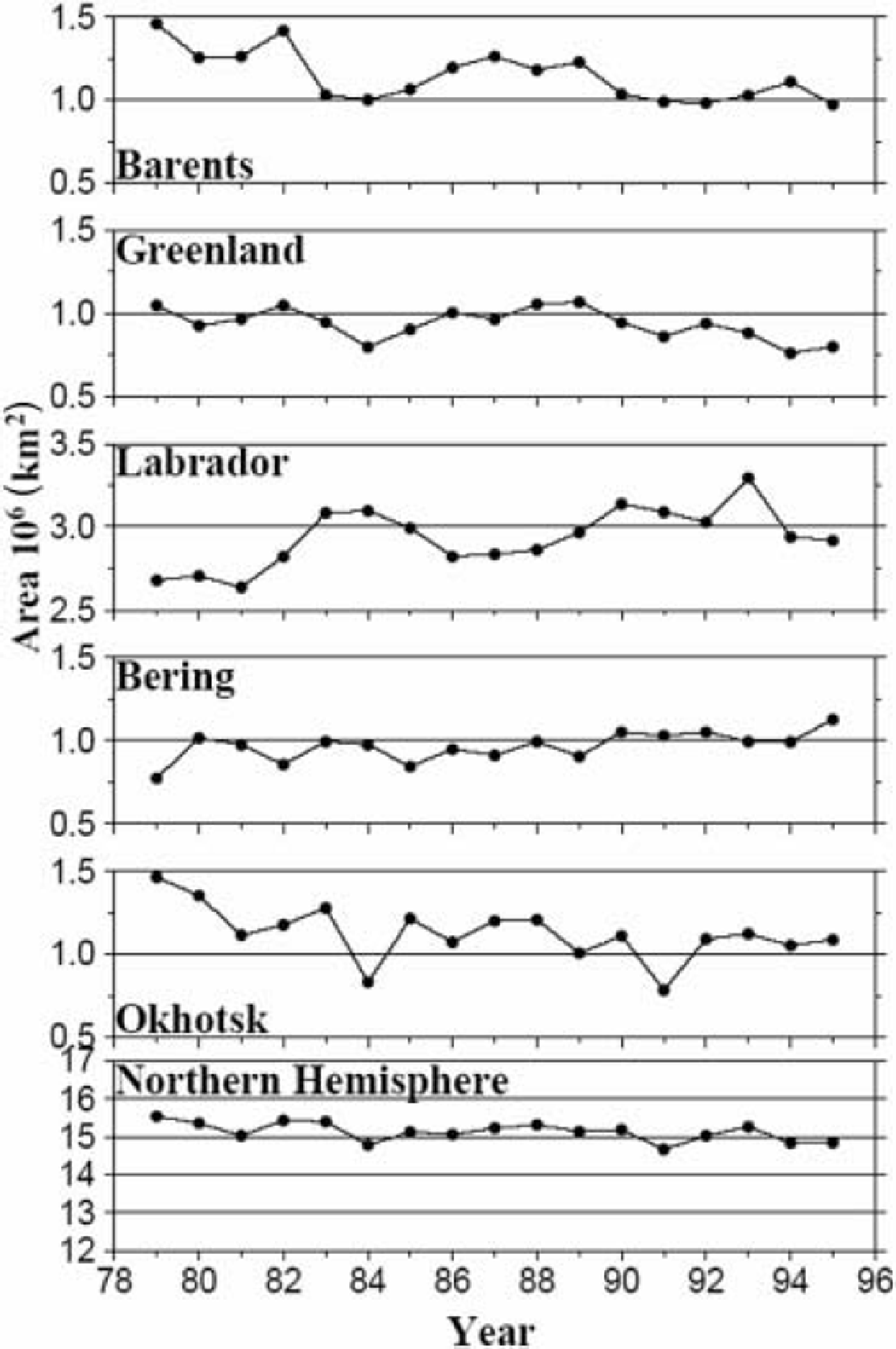
Inspection of Figure 2 shows that both the year-to-year variability and linear trend are smaller in the Greenland and Bering Seas than in the Barents, Labrador and Okhotsk Seas. Obviously, the Greenland and Bering Seas are close to the mean positions of the Icelandic low and Aleutian low, respectively, while the Barents, Labrador and Okhotsk Seas are far away from the two major lows. This may suggest that the interannual variability of sea-ice extent in the Northern Hemisphere is closely related to activities of the Icelandic and Aleutian lows.

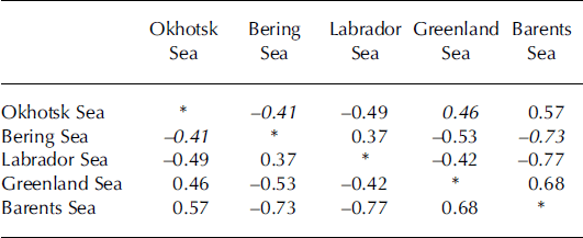
Correlation coefficients (r) of interannual variations of sea-ice extent between the five regions are shown in Table 2. Note that correlations are statistically significant at the confidence levels of 90%, 95% and 99% if correlation coefficients are numerically larger than 0.41, 0.48 and 0.60, respectively. The Barents Sea shows strong positive correlations with the Greenland and Okhotsk Seas, and high negative correlations with the Labrador and Bering Seas. This is consistent with the fact that the Barents, Greenland and Okhotsk Seas show negative trends in ice-extent variation, and the Labrador and Bering Seas positive trends (Fig. 2). The Greenland Sea, located between the Barents and Labrador Seas, shows a positive correlation with the Barents Sea (r= 0.68) and a negative correlation with the Labrador Sea (r= –0.42).

Table 2.

Correlation coefficients of interannual variations of sea-ice extent between the five marginal seas around the Arctic Ocean. Correlations are statistically significant if the correlation coefficients are numerically larger than 0.41, 0.48 and 0.60 at the confidence levels of 90% (italicized values), 95% (bold values) and 99% (underlined values), respectively

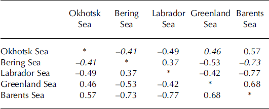
A negative correlation is expected to exist between the Bering and Okhotsk Seas since the Barents Sea has a negative correlation with the Bering Sea (r = –0.73) and a positive correlation with the Okhotsk Sea (r= 0.57). Indeed, a significant negative correlation (r = –0.41) is found between them. This corresponds to occasional out-of-phase fluctuations of sea-ice growth in the Bering and Okhotsk Seas (Reference Cavalieri and ParkinsonCavalieri and Parkinson, 1987). The negative correlation between the western and eastern marginal seas seen in the Pacific basin is also seen in the Atlantic basin, where a strong negative correlation exists between the Barents and Labrador Seas (r = –0.77). In addition, there are significant positive correlations between the Barents and Okhotsk Seas (r = 0.57) and between the Labrador and Bering Seas (r= 0.37). The reason for these across-basin and across-continent teleconnections is discussed later, with emphasis on the role of positions and intensities of the Icelandic low and Aleutian low.

Role of Atmospheric Circulation in Sea-Ice Growth

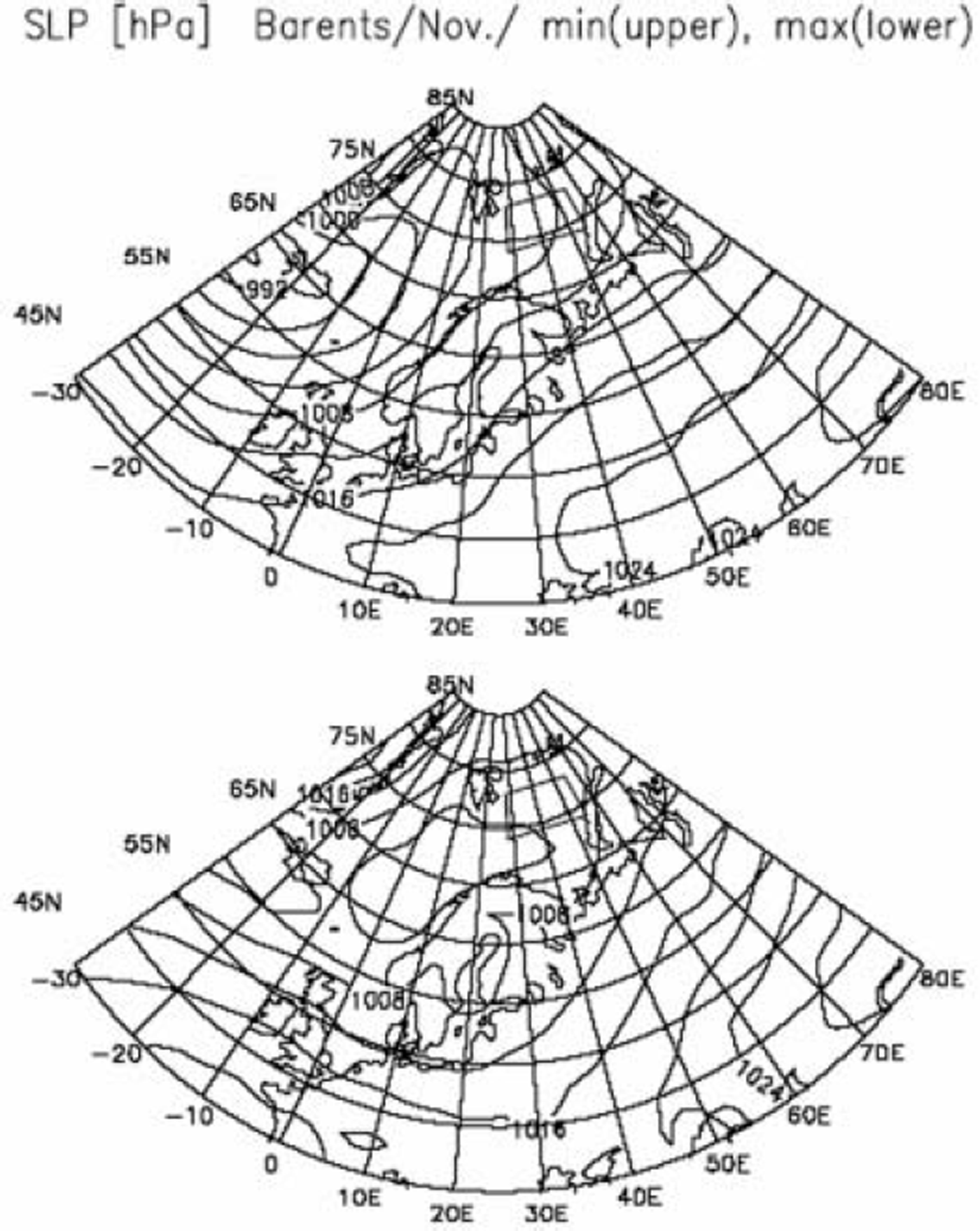
We now proceed to examine composite maps of SLP and T850 fields for various groups of ice growth rate. To begin with, it is noted that composite maps for the cases of low, middle and high growth rates are found to show gradual and coherent changes, though figures are not presented here. Moreover, composite maps for the cases of minimum and maximum growth rates are found to be very similar to those for the cases of low and high growth rates, respectively. We therefore present here only composite maps of for the cases of minimum and maximum growth rates. Figure 3 shows composite maps of SLP fields for the Barents Sea sub-region for November. Wind directions over the sea surface in the Arctic regions can be estimated from the SLP fields by rotating geostrophic wind directions by 30˚ anticlockwise (Reference OverlandOverland, 1985). In the case of minimum growth rate (upper panel), the deep Icelandic low is located to the west of Iceland, and oceanic southwesterly to southerly winds blow over the sub-region. In the case of maximum growth rate (lower panel), the shallow Icelandic low extends eastward to reach the Norwegian/Barents Sea, and consequently weak, cold northeasterly ot easterly winds blow from the Arctic ice field to the sub-region. We conclude that the sea-ice cover in the Barents Sea is advanced by cold-air advection from the Arctic ice field.

Fig. 3.

Composite maps of SLP fields for the Barents Sea sub-region (denoted by the trapezium) for November. The upper panel shows the map for the case of minimum growth rate, and the lower panel for the case of maximum growth rate. The contours are at intervals of 4 hPa.

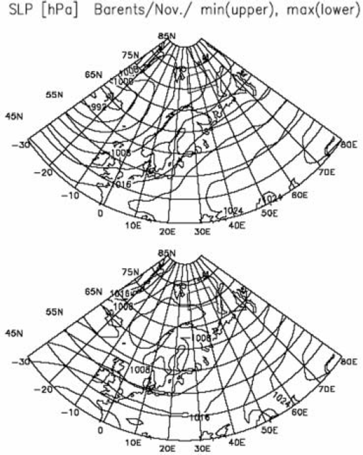
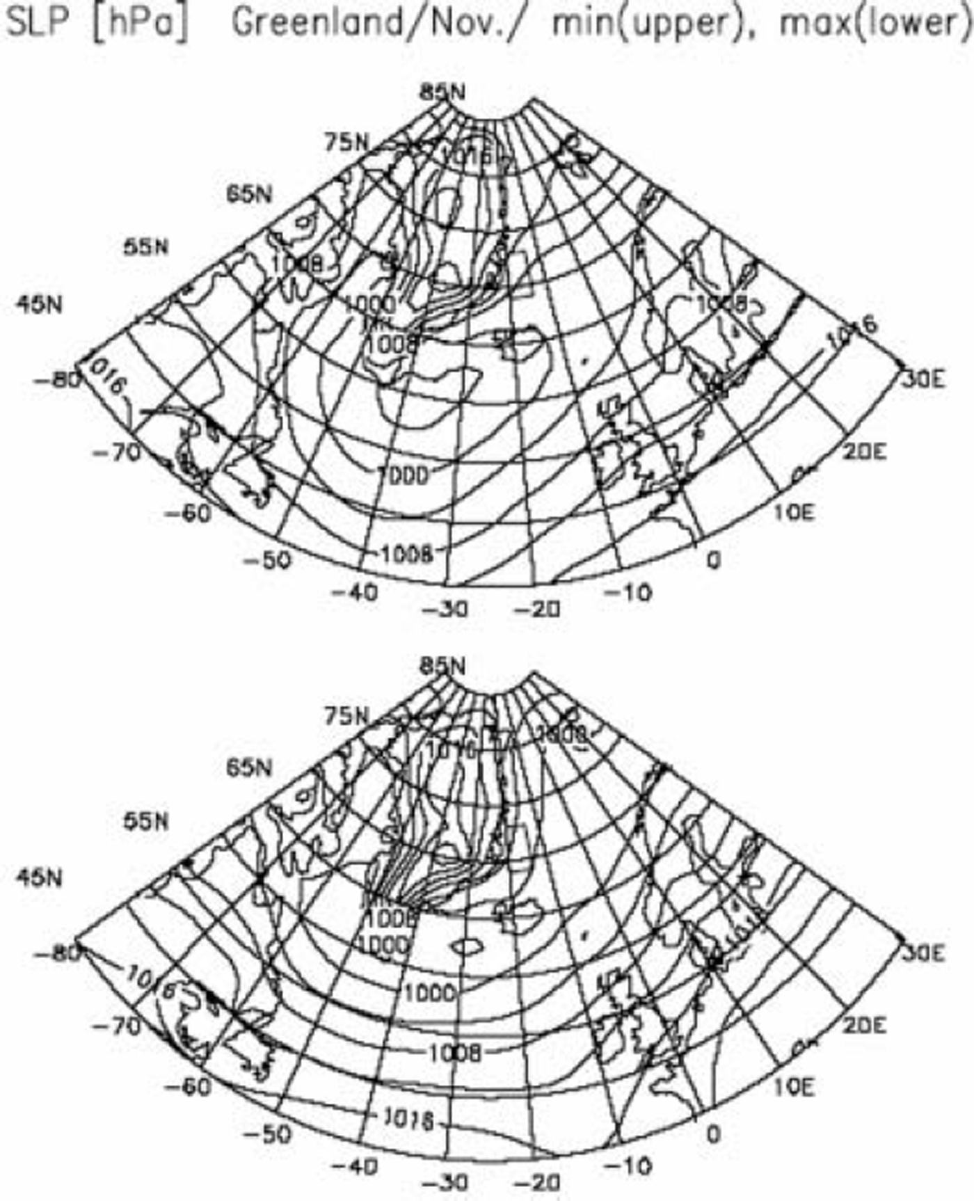
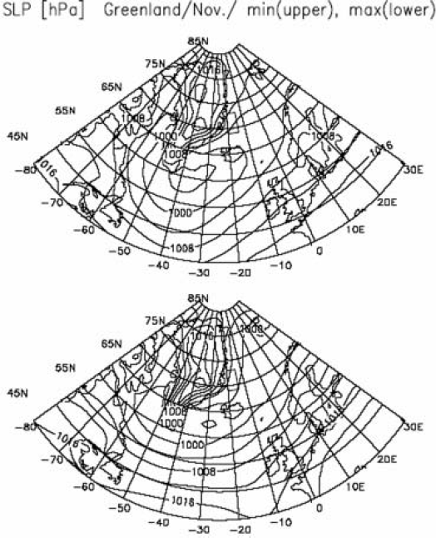
Figure 4 shows composite maps of SLP fields for the Greenland Sea sub-region for November. When growth rates are minimal (upper panel), a deep Icelandic low is located near the southern tip of Greenland and oceanic north to northeasterly winds blow over the sub-region. When growth rates are maximal (lower panel), the Icelandic low is weakened and extends further northeastward to the Norwegian/Barents Sea. In this case, an east–west pressure gradient is established between Greenland and Svalvard, and consequently very cold northwesterly winds blow from Greenland to the sub-region. Reference Shuchman, Josberger, Russel, Fischer, Johannessen and GloersenShuchman and others (1998) also report that cold westerly winds from Greenland cause the Greenland Sea Odden sea ice to grow while warm northerly winds cause it to decay. We conclude that cold-air advection from Greenland to the sub-region is responsible for the sea-ice growth in the Greenland sub-region.

Fig. 4.

Same as Figure 3, but for the Greenland Sea sub-region.

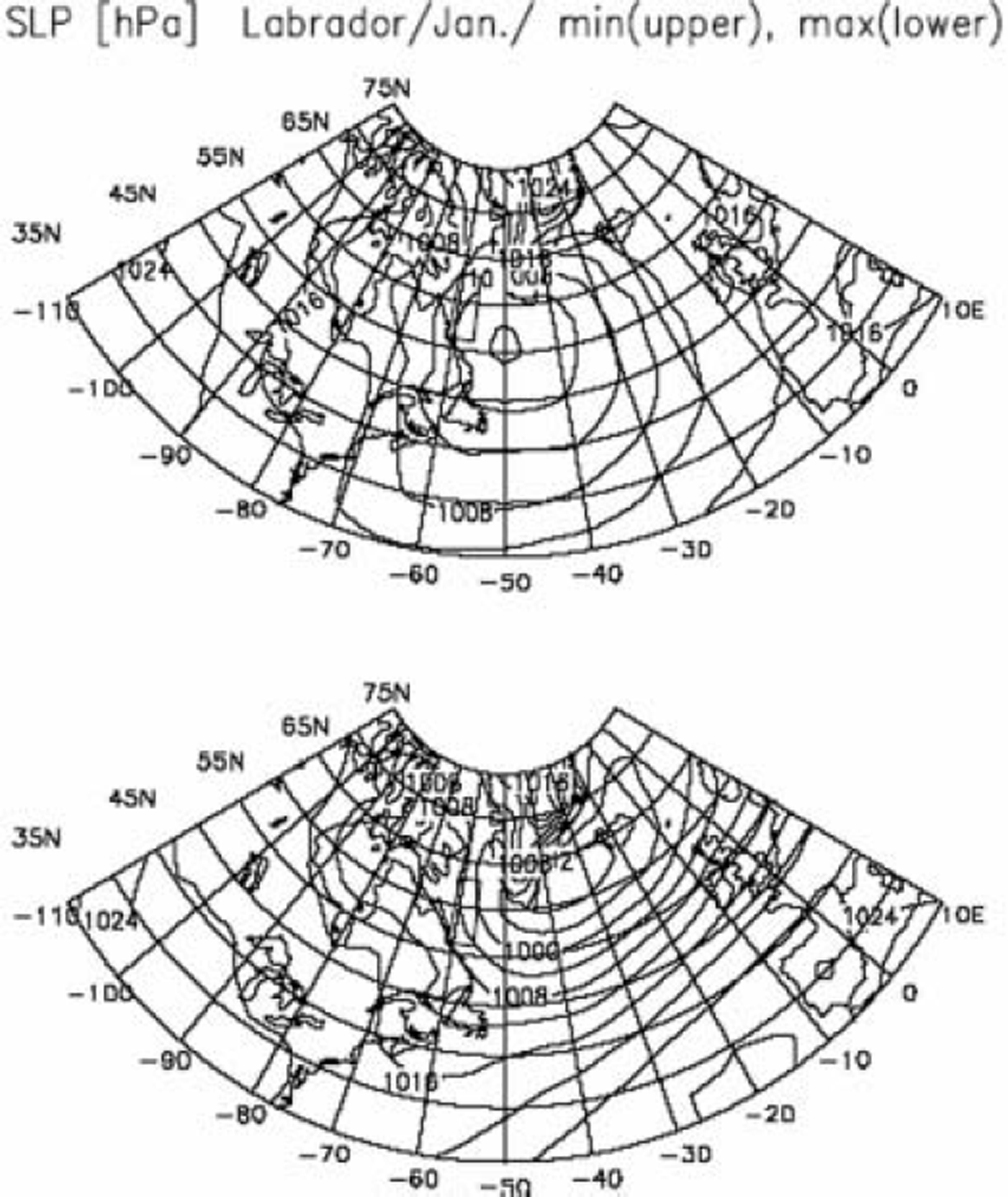
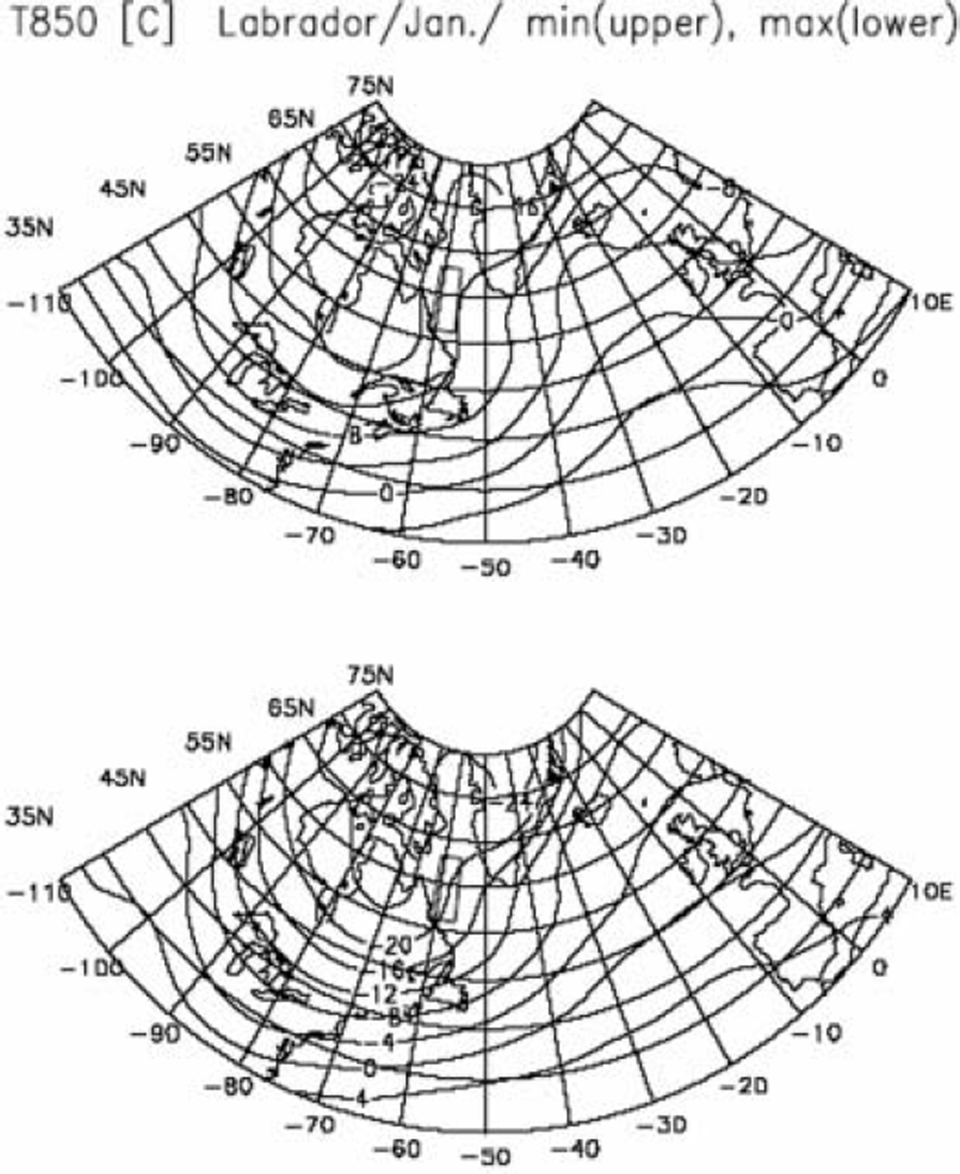
Composite maps of SLP fields for the Labrador Sea subregion for January are shown in Figure 5. In the case of minimum growth rate (upper panel), a moderate Icelandic low is seen between Greenland and the Labrador plateau, which is associated with weak northwesterly winds over the sub-region. (Strong westerly winds blow south of Newfoundland at the 850 hPa surface, though figures are not presented.) In the case of maximum growth rate (lower panel), the Icelandic low is considerably deepened with a minimum pressure <992 hPa, and its central position shifts toward the area between the southern tip of Greenland and Iceland. Reference AgnewAgnew (1993) pointed out that an intensified Icelandic low was associated with heavy sea-ice extent in the Davis/ Labrador Sea, and Reference Parkinson, Cavalieri, Gloersen, Zwally and ComisoParkinson and others (1999) suggested that the positive NAO was associated with the significant sea-ice growth in the Labrador Sea. (Remember that the pressure pattern of a positive NAO is characterized by an intensified Icelandic low located between Iceland and the southern tip of Greenland.) To demonstrate that the intensified Aleutian low brings very cold air from the continent, we show composite maps of T850 fields in Figure 6 for the cases of minimum growth rate (upper panel) and maximum growth rate (lower panel). As expected, air temperatures over Hudson Bay are lower by about 4˚C in the case of maximum growth rate than in the case of minimum growth rate. This indicates that colder air is brought by strong northwesterly winds toward the Labrador sub-region when the sea-ice cover advances. We conclude that sea-ice growth in the Labrador Sea sub-region can be attributed to cold-air advection from the continent.

Fig. 5.

Composite maps of SLP fields for the Labrador Sea subregion (denoted by the trapezium) for January. The upper panel shows the map for the case of minimum growth rate, and the lower panel for the case of maximum growth rate. The contours are at intervals of 4 hPa.

Fig. 6.

Same as Figure 5, but for T850 fields.

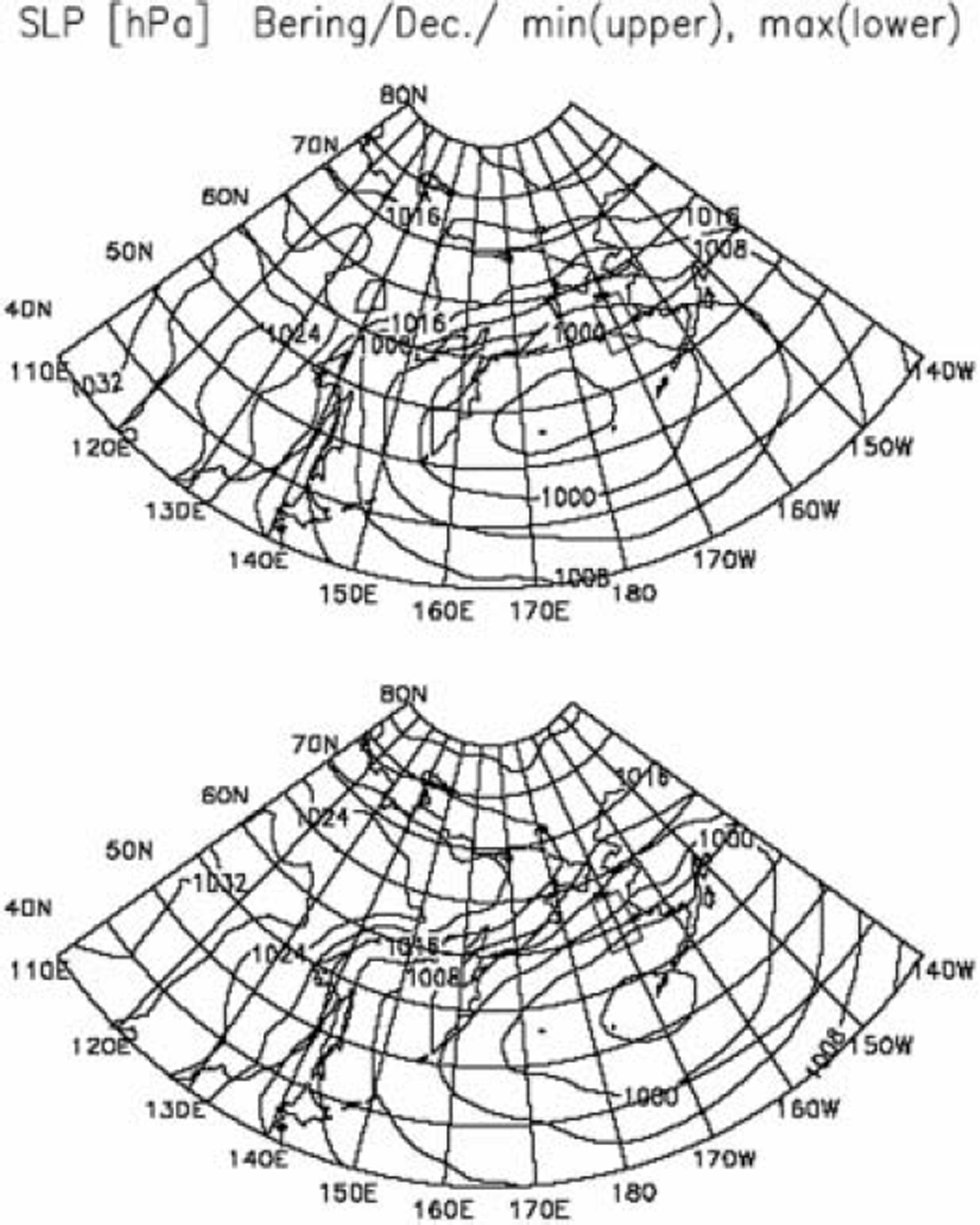
Composite maps of SLP fields for the Bering Sea subregion are shown in Figure 7 for December. When growth rates are minimal (upper panel), a moderate Aleutian low is seen in the central part of the Bering Sea and warm easterly to southeasterly winds blow over the sub-region. When the growth rates are maximal (lower panel), the position of the Aleutian low shifts eastward to reach the Alaska peninsula, and cold northeasterly winds from Alaska blow over the subregion. Again, cold winds from land to ocean are responsible for the sea-ice growth in the Being Sea. This is not inconsistent with Reference AgnewAgnew’s (1993) assertion that heavy ice conditions in the Bering Sea were accompanied by weak secondary lows formed in the Gulf of Alaska.

Fig. 7.

Composite maps of SLP fields for the Bering Sea sub-region (denoted by the trapezium) for December. The upper panel shows the map for the case of minimum growth rate, and the lower panel for the case of maximum growth rate. The contours are at intervals of 4 hPa.

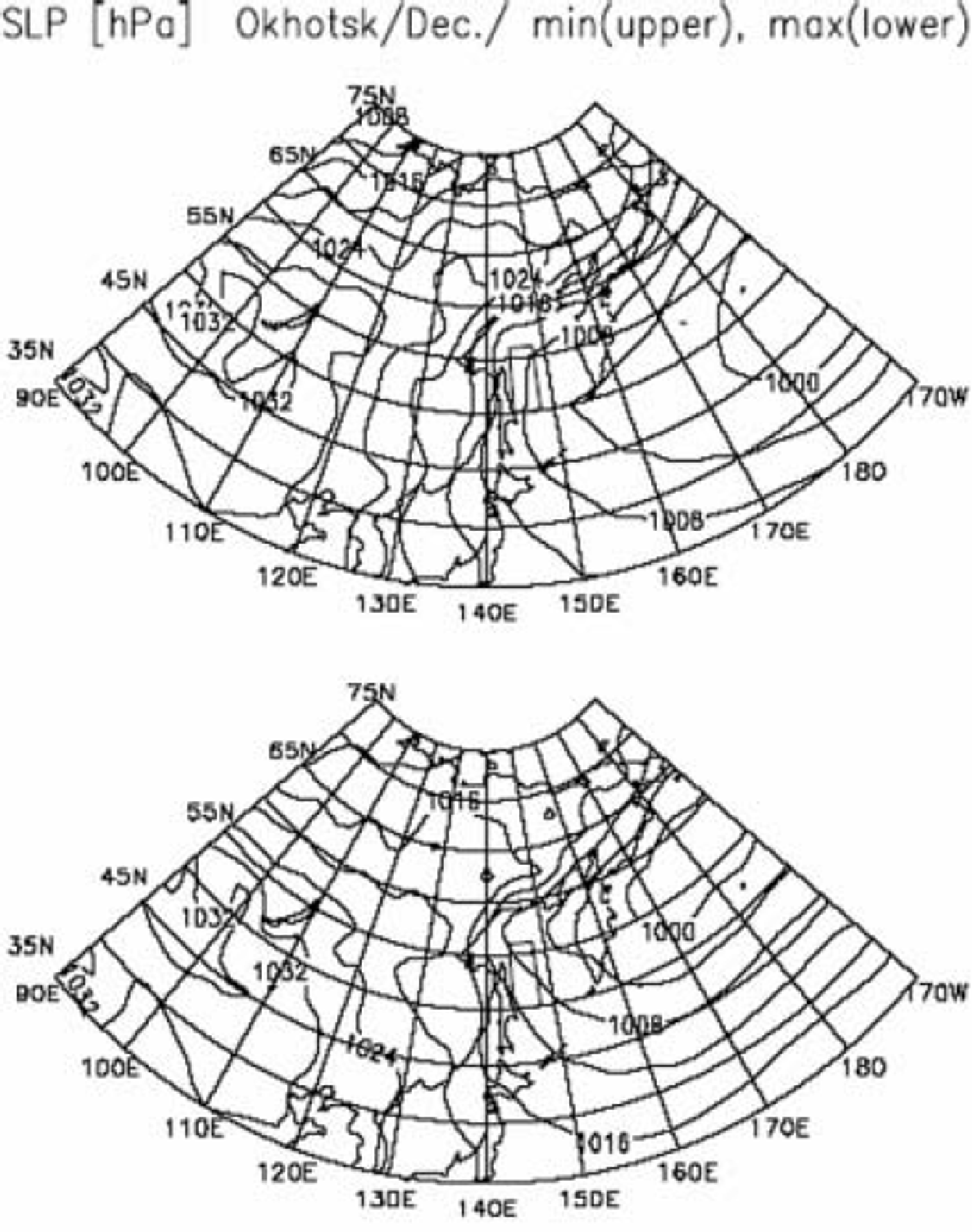
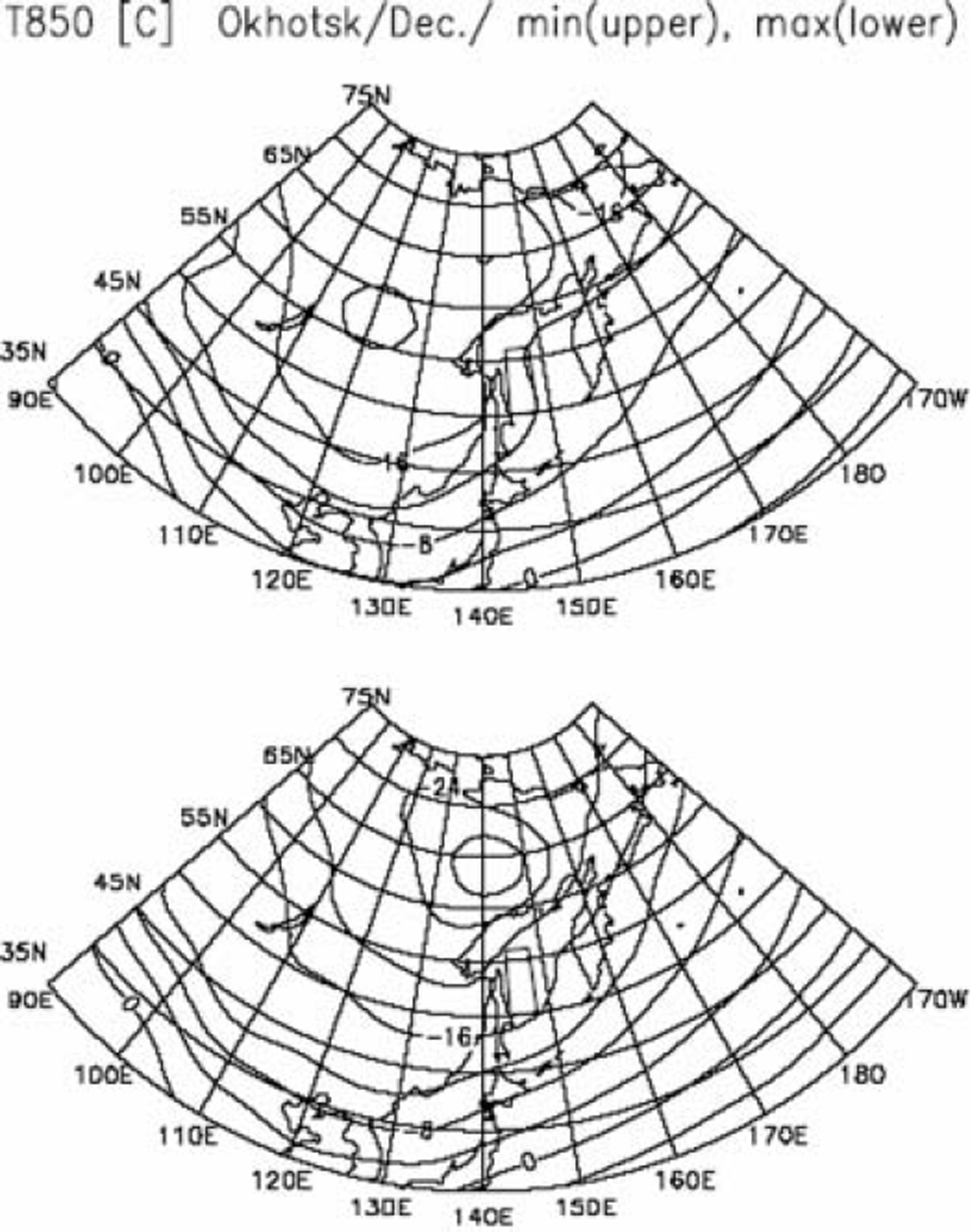
Finally, composite maps of SLP fields for the Okhotsk Sea sub-region are shown in Figure 8 for December. In the case of minimum growth rate (upper panel), a moderate Aleutian low is located far to the east of the Kamchatka peninsula, and northeasterly winds blow over the sub-region. In the case of maximum growth rate (lower panel), the Aleutian low is intensified and its central position shifts northwestward close to the Kamchatka peninsula. As a result, strong northwesterly winds blow from eastern Siberia to the sub-region. The composite maps of T850 fields (Fig. 9) show that northwesterly winds from the continent are 8–12˚C colder in the case of maximum growth rate than in the case of minimum growth rate. We conclude that strong, cold northwesterly winds give rise to the advance of ice extent in the Okhotsk Sea sub-region. Reference Parkinson and GratzParkinson and Gratz (1983), Reference Cavalieri and ParkinsonCavalieri and Parkinson (1987) and Reference ParkinsonParkinson (1990) have also suggested that the positions and intensities of the Siberian high and/or Aleutian low are largely responsible for sea-ice advance/retreat in the Bering and Okhotsk Seas.

Fig. 8.

Same as Figure 7, but for the Okhotsk Sea sub-region.

Although figures are not presented here, a number of composite maps for other months and other sub-regions have been prepared, and all lead to the same conclusion that sea-ice extent is advanced by cold-air advection from the land (or from the Arctic ice field) while it is hardly advanced by warm oceanic air advection. We conclude that growth/decay of sea-ice extent is primarily controlled by atmospheric circulation. Whether this brings cold air or warm air to the marginal sea concerned depends on the activities of the Icelandic low and Aleutian low.

Discussion

Figures 3–9 demonstrate that sea ice advances (or retreats) when cold air (or warm air) is brought to a marginal sea by an atmospheric circulation, and that the atmospheric circulation is largely controlled by the position and intensity of the Icelandic low or Aleutian low. It should be remembered that the activity of the Icelandic low is negatively correlated with that of the Aleutian low (e.g. Reference Wallace and GutzlerWallace and Gutzler, 1981; Reference Van Loon and MaddenVan Loon and Madden, 1983; Reference Honda, Nakamura, Ukita, Kousaka and TakeuchiHonda and others, 2001). Accordingly, a strong (or weak) Icelandic low is expected to be associated with a weak (or strong) Aleutian low. This may result in teleconnections in sea-ice extent between the marginal seas.

Fig. 9.

Same as Figure 8, but for T850 fields.

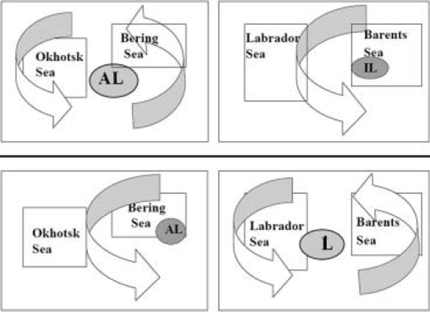
Figure 10 summarizes our conclusions schematically: The upper panel represents the atmospheric circulation in the phase of a strong Aleutian low with a weak Icelandic low. In the Pacific sector (left portion), an intensified and westward-displaced Aleutian low brings cold air from the Eurasian continent to the Sea of Okhotsk, while it brings warm oceanic air to the Bering Sea. In the Atlantic sector (right portion), by contrast, a weakened and eastward-displaced Icelandic low brings warm oceanic air over the Labrador Sea, while it brings cold air from the Arctic ice field (or from Greenland) to the Barents and Greenland Seas. This circulation pattern may result in the advance of sea-ice extents in the Barents and Okhotsk Seas and their retreat in the Labrador and Bering Seas.

Fig. 10.

Schematic diagram for the teleconnections of sea-ice extent and atmospheric circulation. The Labrador Sea represents both the Greenland and Labrador Seas, and IL and AL denote the Icelandic low and Aleutian low, respectively. Arrows represent atmospheric circulations associated with the air-pressure patterns.

The lower panel represents the atmospheric circulation in the phase of a strong Icelandic low with a weak Aleutian low. In the Pacific sector (left portion), a weakened and eastward-displaced Aleutian low brings warm oceanic air to the Sea of Okhotsk, while it brings cold air from Alaska to the Bering Sea. In the Atlantic sector (right portion), by contrast, an intensified and westward-displaced Icelandic low brings cold air from the American continent to the Labrador Sea, while it brings warm oceanic air to the Barents and Greenland Seas. This circulation pattern may result in the advance of sea-ice extents in the Labrador and Bering Seas and their retreat in the Barents and Okhotsk Seas. Remember that these are exactly the same features that have been demonstrated in Figures 3–8. We conclude that the teleconnections in sea-ice extent discussed before are caused by interannual variabilities of the positions and intensities of the Icelandic low and Aleutian low.

The above conclusions suggest that the linear trends of sea-ice extent in the marginal seas (see Fig. 2) must be associated with linear trends in the intensities of the Icelandic and Aleutian lows. In other words, the positive trend of sea-ice extent in the Labrador Sea and the negative trends in the Barents and Greenland Seas must be associated with an increasing trend of the Icelandic low (or of NAO). At the same time, the positive trend of sea-ice extent in the Bering Sea and the negative trend in the Sea of Okhotsk must be associated with a decreasing trend of the Aleutian low. Indeed, Reference HurrellHurrell (1995, 1996) showed an increase in the NAO index since the 1960s, and Reference Overland, Adams and BondOverland and others (1999) showed a strengthening of the Icelandic low and a weakening of the Aleutian low during a recent decade. Reference Tachibana, Honda and TakeuchiTachibana and others (1996) also discussed the recent weakening of the Aleutian low in connection with the decrease in sea-ice extent in the Sea of Okhotsk. In short, all the above studies are consistent with our conclusions.

Whether or not the sea-ice extent is still increasing in the Labrador and Bering Seas and decreasing in the Barents, Greenland and Okhotsk Seas after 1995 is an interesting question. In 2002, the dataset of the Northern Hemisphere EASE-GRID Weekly Snow Cover and Sea Ice Extent was revised and extended until June 2001. Note that a new microwave radiometer F13 was adopted after 1995, and the algorithm and quality check to determine the sea-ice extent have also been modified in this revision (for details see Reference Armstrong and BrodzikArmstrong and Brodzik, 2002b). In Figure 11, interannual variations of 3monthly (January–March) means of sea-ice extent, calculated from the new dataset, are shown for the period 1990–2001. Comparison with Figure 2 shows that general tendencies of variation have been reversed since the period 1994–96. For example, the positive trends for the Labrador and Bering Seas seem to have changed to negative trends, and the negative trend for the Sea of Okhotsk to a positive trend. The negative trends for the Barents and Greenland Seas also seem to have changed to positive trends, though variations of a smaller timescale are seen as well. In addition, the negative trend for the whole Northern Hemisphere seems to have become stationary. When we combine the two datasets, the distinctive changes for the Barents, Greenland and Okhotsk Seas around 1995 reduce the value of the correlation coefficient between the marginal seas, but most of the teleconnection patterns shown in Table 2 are still statistically significant at the 85% confidence level.

Fig. 11.

Updated interannual variations of the 3 monthly (January– March) means of sea-ice extent for the years 1990–2001. The values are derived from Northern Hemisphere.

Finally, we briefly discuss the possible controlling factor for the advance/retreat of sea-ice cover in the Arctic marginal seas. Needless to say, sea ice forms when seawater temperature drops below the freezing point (about –1.8˚C). Reference Tabata, Noguchi and SaitoTabata and others (1980) found a strong correlation between the sea-ice thickness in the Sea of Okhotsk and the accumulated sub-zero temperatures (degree-days). In their study of intra-annual and interannual variability of the Greenland Sea Odden sea-ice feature, Reference Shuchman, Josberger, Russel, Fischer, Johannessen and GloersenShuchman and others (1998) concluded that the key meteorological parameters responsible for rapid ice formation/decay are, in order of importance, air temperature, wind speed and wind direction. On the other hand, Reference Parkinson, Cavalieri, Gloersen, Zwally and ComisoParkinson and others (1999) suggested that the airflows associated with Icelandic lows sometimes decreased ice extents by pushing the ice toward the Greenland coast, and sometimes increased ice extents by spreading the ice southward. Recently, Reference Kimura and WakatsuchiKimura and Wakatsuchi (1999, Reference Kimura and Wakatsuchi2001) demonstrated high correlations between the sea-ice advance/retreat and geostrophic wind speed in the Arctic marginal seas and concluded that the advance/retreat of ice cover is primarily controlled by the sea-ice drift due to winds.

In view of the above discussions, it is important to note that wind speed and/or wind direction is generally highly correlated with air temperature in winter. This implies that, even if wind speed is highly correlated with sea-ice growth, it does not necessarily follow that sea ice grows or expands by ice drift since sea ice is also likely to grow by atmospheric cooling by strong winds. We must distinguish the two processes clearly. In this respect, we should remember that sea-ice cover generally advances from north to south and/or from land to ocean in the growth season, and retreats in the reverse order in the decay season (see Fig. 2; Reference Parkinson, Comiso, Zwally, Cavalieri, Gloersen and CampbellParkinson and others, 1987; Reference Gloersen, Campbell, Cavalieri, Comiso, Parkinson and ZwallyGloersen and others, 1992). This implies that the ice-cover season is longer in inshore than in offshore regions and that, consequently, sea ice is thicker in inshore regions. It seems clear that this heterogeneity in ice thickness in the wind direction cannot be caused by sea-ice drifts by wind, because the wind drift would homogenize the ice thickness downwind. In addition, inshore winds, which are supposed to push ice floes coastwards during the ice-decay season, are not observed in a statistical sense in most of the Arctic marginal seas.

The results of our analysis suggest that sea-ice covers in the marginal seas grow downwind through cold-air advections from the continents or from the cold Arctic ice field. In this connection, we note that an important role of air-mass transformation with fetch (the downwind distance from a coast) in the process of atmospheric cooling has been discussed in detail (Reference Rikiishi and TakatsujiRikiishi and Takatsuji, 2006).