Introduction
The polar ionosphere is known to be extremely irregular both spatially and temporally, with a wide range of structures related to complex dynamics and particle precipitation phenomena. Many polar ionograms show that the echo pulse reflected from the F2 layer has a much longer duration (10 times) than the transmitted pulse. This phenomenon is usually referred to as spread-F and many studies have described its morphological and dynamic peculiarities (e.g. Penndorf Reference Penndorf1962). Spread-F is caused by scattering from irregularities in the ionosphere across the entire radiation angle of the antenna. In the polar ionosphere such irregularities are field aligned and occur against a background of Travelling Ionospheric Disturbances (TIDs), with horizontal sizes ranging from several tens of meters to about 40 km (Nekrasov et al. Reference Nekrasov, Shirochkov and Shumilov1982). Certain types of spread-F are caused by radio aurora, this being the radar signature of the ionization associated with auroral phenomena (Davies Reference Davies1990).
Another important feature of polar ionograms is the so-called Z-ray, which is a third trace appearing on ionograms, spaced in critical frequency from the ordinary ray (O-ray) by approximately half the electron gyrofrequency. A phenomenon that must be considered when dealing with Z-ray ionograms is resolved frequency spreading. In these cases, ionograms present a duplicate ordinary trace representing reflections from markedly different directions, with the spread in critical frequency indicating a horizontal gradient in the peak electron density (Piggott & Rawer Reference Piggott and Rawer1972). An ionogram record in which the satellite trace is spaced in critical frequency from the O-ray by half of the electron gyrofrequency, as would be expected of a Z-ray, can lead to an uncertain interpretation of the radio propagation conditions. However, this ambiguity can be resolved by considering that if a satellite trace characterizes the O-ray, a corresponding satellite trace should also characterize the extraordinary ray (X-ray), at least in some part of the record (Bowman Reference Bowman1960).
In the ionograms recorded at the Mario Zucchelli Station (74.7°S, 164.1°E), Terra Nova Bay (TNB), Antarctica, the Z-ray appears as a clean single-line trace only in a minority of cases. At other times this trace is duplicated in the same way as the O- and X-ray traces are duplicated (resolved frequency spreading). In many cases it apparently consists of a number of traces so close that the Z-ray appears diffused. It is also important to bear in mind that the mechanism underlying the reflection of this ray involves the presence of irregularities, which are also responsible for spread-F (Bowman Reference Bowman1960, Papagiannis & Miller Reference Papagiannis and Miller1969).
The problem of an appropriate labelling of ionograms with continuous transitions between the different possible conditions (Z-ray, resolved spread-F, unresolved spread-F) poses a challenge for any automatic scaling software (Reinisch & Huang Reference Reinisch and Huang1983, Fox & Blundell Reference Fox and Blundell1989, Igi et al. Reference Igi, Nozaki, Nagayama, Ohtani, Kato and Igarashi1993, Tsai & Berkey Reference Tsai and Berkey2000, Reinisch et al. Reference Reinisch, Huang, Galkin, Paznukhov and Kozlov2005, Zabotin et al. Reference Zabotin, Wright and Zhbankov2006, Ding et al. Reference Ding, Ning, Wan and Liu2007). In this work a possible solution for the automatic detection of these conditions is presented, with the aim of improving the performance of the Autoscala program (Scotto & Pezzopane Reference Scotto and Pezzopane2002, Pezzopane & Scotto Reference Pezzopane and Scotto2004) in high latitude applications.
Finally, another important phenomenon that is frequently observed at high latitude is the D region absorption event, which can lead to a complete disappearance of any overlying region echo from the ionogram record. This is similar to what occurs at low and mid latitudes during a Sudden Ionospheric Disturbance (SID), when X-rays penetrate to the D region releasing electrons with increasing absorption, resulting in short wave radio blackout. In addition to SIDs, at polar latitudes short wave radio fadeout can be due to Polar Cap Absorption (PCA). These events result from the D region ionizing effect of high-energy protons emitted during solar flares which spiralize around and down the magnetic field lines of the Earth penetrating into the atmosphere near the magnetic poles.
Although a PCA event can last any time from about one hour to several days, while a SID lasts 30–60 min, both phenomena appear on ionosonde records as blank ionograms, indicating absorption effects at lower altitudes due to increased ionization in the D region. These ionograms constitute another challenge for automatic scaling software because they need to be identified and distinguished from cases characterized by spread-F features, and from those in which only the F2 part of the trace is not clearly recorded.
This paper first describes the algorithms added to Autoscala to address the high latitude ionogram features mentioned above, and then some results from the application of this version of Autoscala to a series of ionograms recorded by the AIS-INGV (Advanced Ionospheric Sounder-Istituto Nazionale di Geosifica e Vulcanologia) ionosonde (Zuccheretti et al. Reference Zuccheretti, Tutone, Sciacca, Bianchi and Arokiasamy2003) installed at TNB.
The method applied by Autoscala
The techniques described in this work to detect D region absorption events, spread-F, and Z-rays are evolutions of the basic algorithm on which Autoscala was originally designed in order to identify the F2 layer (Pezzopane & Scotto Reference Pezzopane and Scotto2005, Reference Pezzopane and Scotto2007). In this algorithm, the ionogram is initially memorized by Autoscala as a matrix A of m rows and n columns, whose values are defined by the following formulas:

and

where ff, f 0, Δf, h ′f, h ′0, and Δh ′ are respectively final frequency, initial frequency, frequency step, final virtual height, initial virtual height, and virtual height resolution of the sounding. h ′0 and Δh ′ are fixed values depending upon the design of the ionosonde. For the AIS-INGV h ′0 is 90 km and Δh ′ is 4.5 km. The element aij (with i = 1,…, m and j = 1,…, n) of the matrix A is an integer varying from 0 to 254, this value being proportional to the echo amplitude received by the ionosonde. The automatic scaling procedure starts by defining two empirical curves T O and T X that are able to fit the typical shapes of the F2 ordinary and extraordinary traces. The curves are expressed in the following parametric forms:
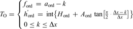
for the curve used for the investigation of the O-ray, and
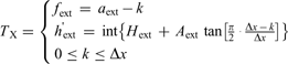
for the curve used for the investigation of the X-ray. In Eq. (2a) & (2b) the frequencies and the virtual heights of T O and T X are expressed as integers and correspond to the indices i and j of entries aij of matrix A. The parameters defining the two curves are:

H ord and H ext are integers varying from 1 to (m-30) and correspond to the values of the horizontal asymptote for T O and T X. a ord and a ext are integers varying from 1 to n, with the condition a ord < a ext, and correspond to the values of the vertical asymptote for T O and T X. A ord and A ext are two decimal coefficients. Δx is an integer varying from 6 to 30, representing the frequency interval, expressed in pixels, where T O and T X develop. Once Δx is set, the curves start from frequencies (a ord - Δx) and (a ext - Δx) and extend up to a ord and a ext as integer k varies from 0 to Δx. For small values of a ord and a ext it may happen that f ord and f ext are negative, but these values are intercepted and neglected by the algorithm as they correspond to negative values of the frequency.
For each pair of curves T O and T X the local correlation C(H ord, H ext, a ord, a ext, A ord, A ext, Δx) with the recorded ionogram is calculated and the pair of curves T O and T X with the maximum value C max of C are then selected. If C max is greater than a fixed threshold C t the selected curves are considered as representative of the F2 trace. foF2 is thus obtained as the frequency of the vertical asymptote a ord of T O, while MUF(3000)F2 is numerically calculated by finding the transmission curve tangent to T O. On the contrary, if C max does not exceed C t the routine assumes that the F2 trace is not present in the ionogram.
D region absorption event ionogram identification
As noted above, a D region absorption event features as a blank ionogram in ionosonde data, and this absorption is due either to a SID or a PCA. In order to intercept these cases, for each pair of curves T O and T X, besides the local correlation C and index I was computed, which makes allowance both for the number of matched points and their amplitude (from 0 to 254). Next, the number N of pairs of curves for which I is greater than a fixed threshold I t was computed.
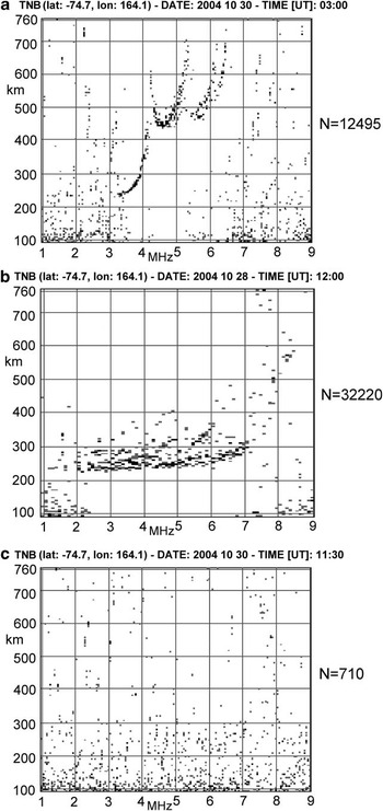
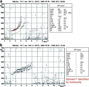
Figure 1 shows a well defined trace ionogram, a spread-F ionogram, and a blank ionogram for which N is equal to 12495, 32220, and 710 respectively. A low N value for blank ionograms is quite a consistent characteristic and can be used to intercept these cases. Therefore, a threshold N t for N was empirically set, so that cases with N < N t are interpreted as blank ionograms.
a. A well-defined ionogram trace, b. a spread-F ionogram, and c. a blank ionogram, for which the parameter N was equal to 12495, 32220, and 710 respectively. Low N values for blank ionograms is quite a systematic characteristic and was used to intercept these cases, fixing an empirical threshold of N t = 3000.

Z-ray identification
In order to identify potential triple splitting (Bowman Reference Bowman1960) characterizing a recorded ionogram trace, in addition to the empirical curves of Eq. (2a) & (2b), the automatic scaling procedure defines a third empirical curve T Z expressed in the following parametric form:
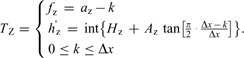
Three new parameters, H z, a z, and A z, are then defined. H z is an integer varying from 1 to (m - 30) and corresponds to the value of the horizontal asymptote for T Z. a z is an integer varying from 1 to n, with the condition a z < a ord, and corresponds to the value of the vertical asymptote for T Z. A z is a decimal coefficient. Once Δx is set, the curve of Eq. (4) starts from the frequency (a z - Δx) and extends up to a z as integer k varies from 0 to Δx. For small values of a z it may happen that f z is negative, but this value is intercepted and ignored by the algorithm.
For each tern of curves T Z, T O, and T X, the local correlation C(H z, H ord, H ext, a z, a ord, a ext, A z, A ord, A ext, Δx) with the recorded ionogram is calculated making allowance for both the number of matched points and their amplitude, and the tern of curves T Z, T O, and T X with the maximum value C max of C is then selected. If C max is greater than a fixed threshold C tz, under the condition C tz > C t, the algorithm interprets the presence of triple splitting in the ionogram and the selected curves as representative of the Z-ray, O-ray, and X-ray respectively. On the contrary, if C max does not exceed C tz then the routine assumes that triple splitting is not present.
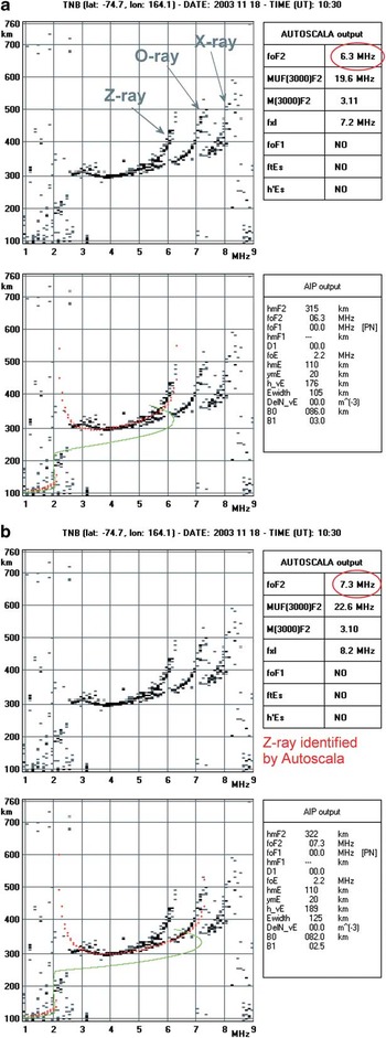
The introduction of a third curve for identifying potential triple splitting gave quite good results and in this respect Fig. 2 shows the autoscaling performed by Autoscala on an ionogram characterized by a triple splitting before and after defining the third empirical curve T Z. In Fig. 2 an estimation of the vertical electron density profile (Scotto Reference Scotto2009) is also shown.
Ionogram showing triple splitting and the corresponding autoscaling performed by Autoscala a. before, and b. after defining a third empirical curve T Z. The top panels contain the original recorded ionogram and the main ionospheric characteristics given as output by Autoscala (“AUTOSCALA output” table). Red ellipses highlight the values of autoscaled foF2 values before and after defining T Z. Red and green curves in the bottom panels represent the reconstructed O-ray and the corresponding vertical electron density profile, respectively. The “AIP output” table gives the parameters used by Autoscala to estimate the vertical electron density profile associated with the restored ordinary trace.

Spread-F identification
In order to detect a spread-F condition in ionograms, not only the pair of curves with maximum C value are taken into account, but all curves with a local C correlation exceeding a threshold C ts. All these pairs are considered, retaining the associated parameters in corresponding arrays. Attention is then focused on the parameter a ord, which is associated with the vertical asymptote of T O. A histogram is defined, reporting the number of curve pairs exceeding C ts as a function of a ord.
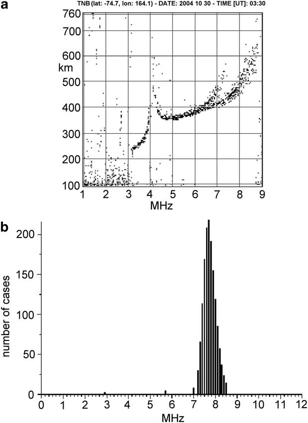
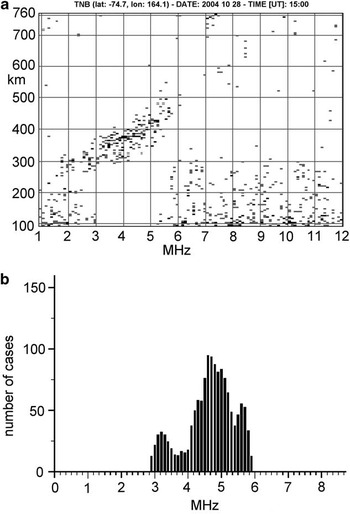
Figure 3a shows an ionogram in which the F2 trace is well defined, and Fig. 3b the corresponding histogram. It can be seen that in this case the distribution presents a well defined single maximum. Figure 4a shows an ionogram in which the F2 trace is not well defined due to the presence of spread-F. The corresponding histograms, reported in Fig. 4b, show multiple maximums. This behaviour is quite systematic and can be used as a criterion to differentiate ionograms featuring spread-F from well defined trace ionogram.
a. Ionogram for which the F2 trace is well defined, and b. the corresponding histogram, showing a well defined single maximum.
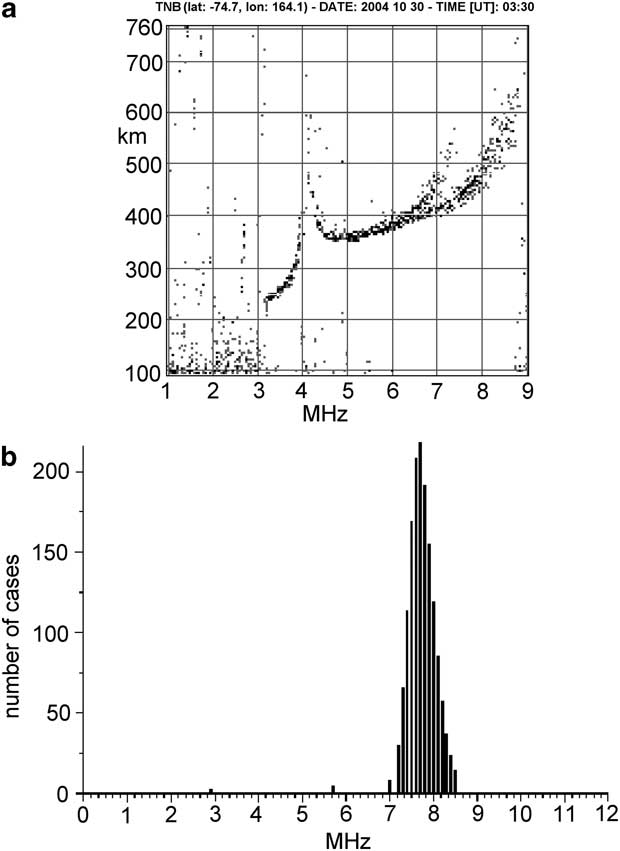
a. Ionogram for which the F2 trace is not well defined due to the presence of spread-F, and b. the corresponding histogram showing multiple maximums.

Critical cases
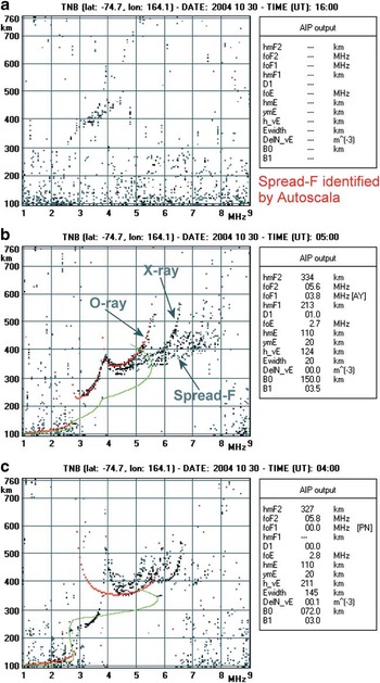
Figure 5 shows two examples of the behaviour of Autoscala when applied to non-critical polar ionograms. Figure 5a shows a sufficiently defined trace and Autoscala was able to perform good scaling of the main standard International Union of Radio Science (URSI) parameters, also providing a reliable estimation of the vertical electron density profile. Figure 5b shows an ionogram with a noticeable spread-F and this was correctly intercepted by the software which generated no output data.
a. Sufficiently defined ionogram for which Autoscala was able to perform a good scaling providing a reliable estimation of the vertical electron density profile (in red the restored O-ray and in green the corresponding vertical electron density profile). b. Spread-F ionogram correctly intercepted by the software and producing no output data. Refer to Fig. 2 for the significance of the “AIP output” table.

By contrast, Fig. 6 shows some examples of the behaviour of Autoscala with some critical ionograms, which exhibit intermediate features and consequently represent a challenge for the software. Figure 6a is an example of an ionogram in which the action of D region absorption is observable, although part of the F2 trace is still present. This trace is not clearly defined but a marked spread-F condition cannot be assumed. In this case the ionogram was automatically scaled as spread-F, although classification as a blank ionogram would have been more appropriate.
a. Ionogram in which the action of D region absorption prevents observation of the overlying ionospheric layer echoes except part of the F2 trace. This was automatically scaled as spread-F although a classification as a blank ionogram would have been more appropriate. b. Spread-F conditions not impeding a correct scaling of the ionogram which was properly autoscaled. c. Spread-F conditions impeding correct scaling of the ionogram which was incorrectly considered as having a well-defined trace, and for which an unrealistic vertical electron density profile was computed. Red and green curves in b. and c. represent the reconstructed O-ray and the corresponding vertical electron density profile, respectively. Refer to Fig. 2 for the significance of the “AIP output” table.

Figure 6b & 6c show two different kinds of spread-F ionogram. The second, unlike the first, prevents scaling of the ionogram. While the Fig. 6b ionogram was correctly classified, the Fig. 6c ionogram was incorrectly interpreted as having a well defined trace, producing an unrealistic vertical electron density profile.
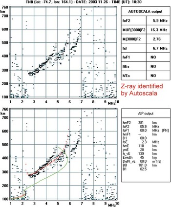
As regards Z-ray identification, it can happen that the algorithm interprets a Z-ray to be present when the trace is more probably characterized by a spread-F phenomenon (see Fig. 7), but without doubt this distinction would be very difficult even for an expert operator.
Ionogram identified by Autoscala as a case of triple splitting but more probably characterized by a spread-F phenomenon. Red and green curves in the bottom panel represent the reconstructed O-ray and the corresponding vertical electron density profile, respectively. Refer to Fig. 2 for the significance of the “AUTOSCALA output” and “AIP output” tables.

Overall, in a preliminary data analysis performed on 416 ionograms recorded at the Mario Zucchelli Station, there were only 25 definitely wrong cases.
Summary
The high latitude ionosphere is extremely unstable, often characterized by strong D region ionizations, causing absorption events, and by the presence of irregularities that can cause rapid changes in both the amplitude and phase of radio signals passing through them, producing scintillations that seriously degrade trans-ionospheric radio communications. Blank ionograms are the manifestation of absorption events, while Z-ray and spread-F signatures on ionograms are the signs of ionospheric irregularities. An automatic system that was capable of reliably monitoring such features in real time would be very advantageous.
This paper described some new procedures added to Autoscala to address problems with high latitude ionograms. The procedures performed reasonably well, while simultaneously highlighting certain critical cases that can degrade their performance.
Acknowledgements
The constructive comments of the reviewers are gratefully acknowledged.