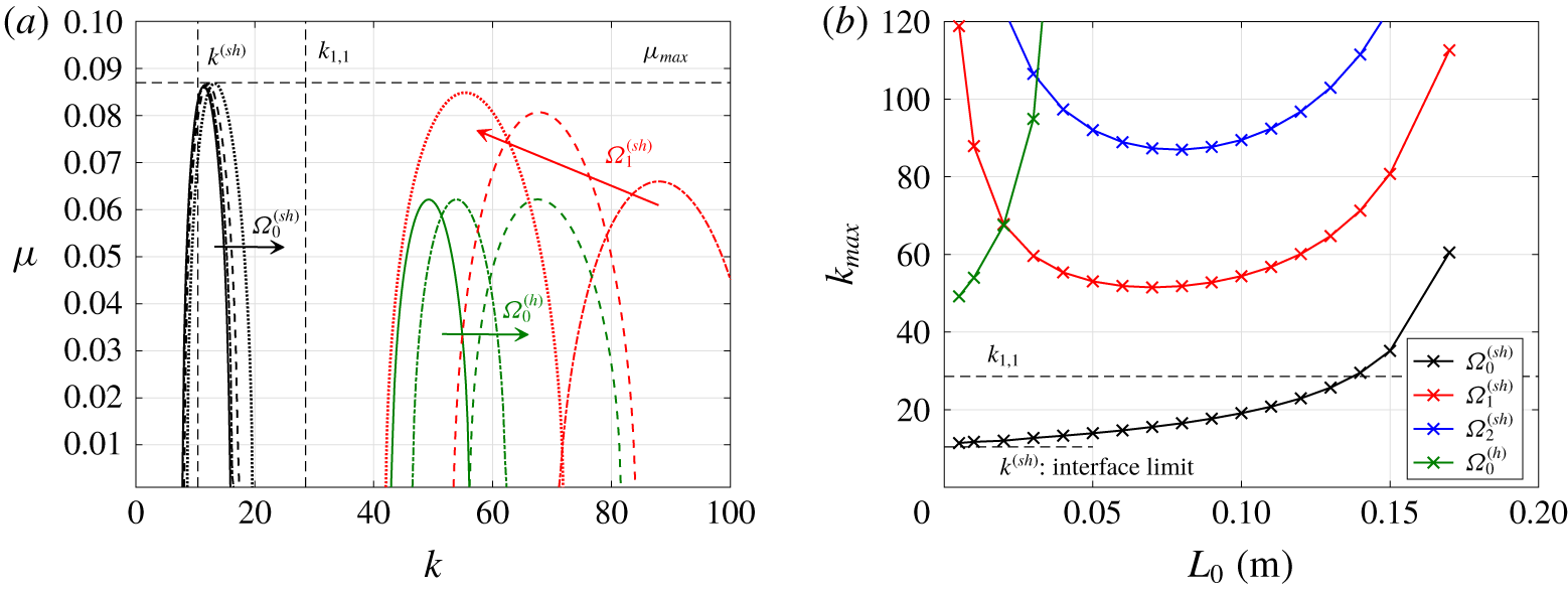
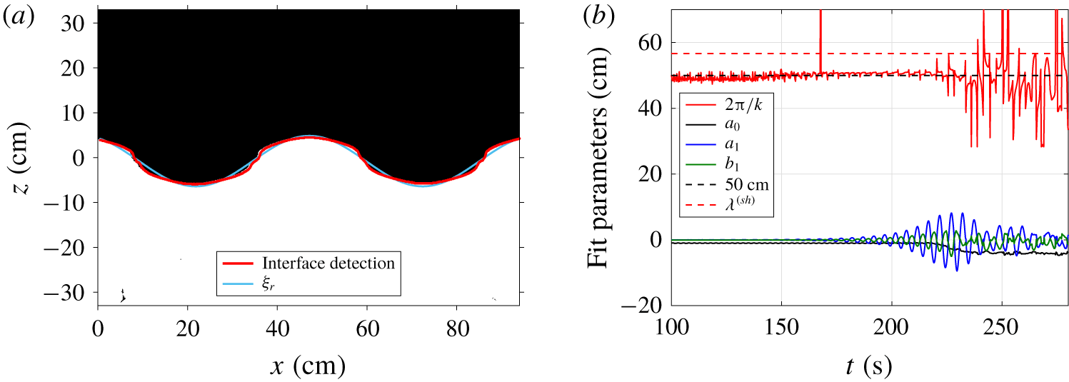
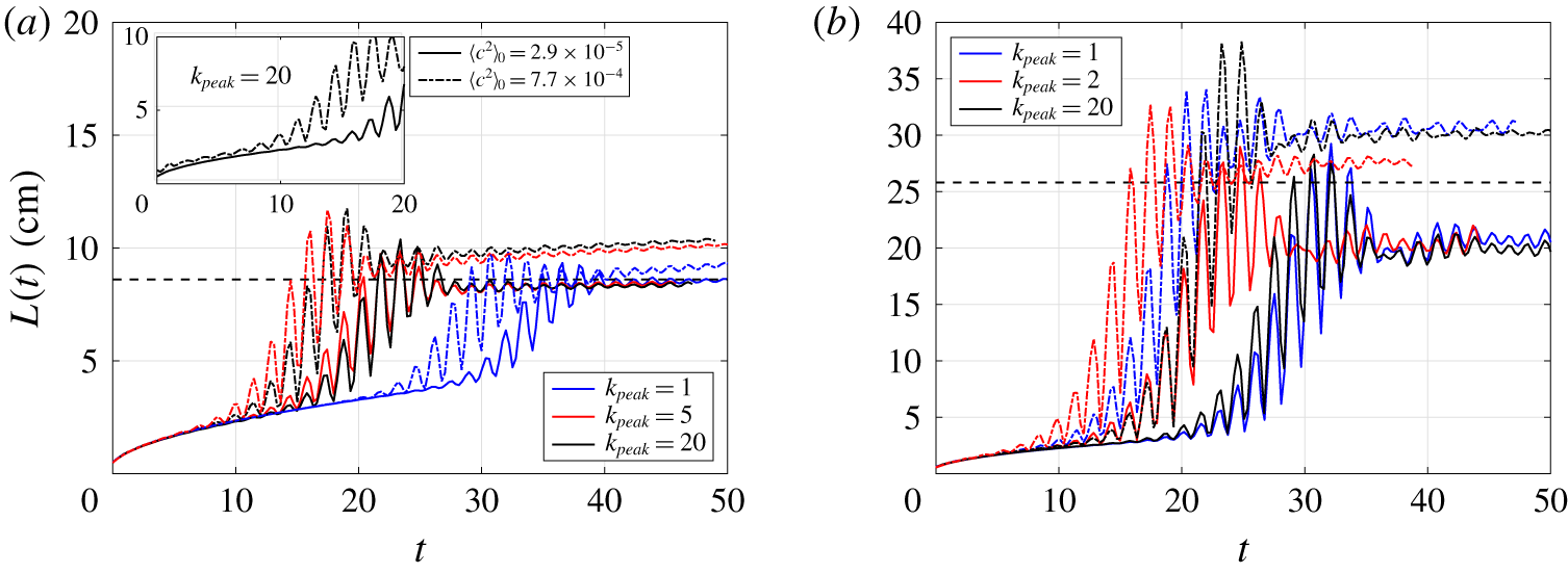
1 Introduction
The statically stable interface between two immiscible fluids of densities  $\unicode[STIX]{x1D70C}_{1}$ and
 $\unicode[STIX]{x1D70C}_{2}<\unicode[STIX]{x1D70C}_{1}$ can be destabilised under periodic vertical acceleration, as a result of the Faraday instability (Faraday Reference Faraday1831). For specific values of the control parameters – the Atwood number
 ${\mathcal{A}}=(\unicode[STIX]{x1D70C}_{1}-\unicode[STIX]{x1D70C}_{2})/(\unicode[STIX]{x1D70C}_{1}+\unicode[STIX]{x1D70C}_{2})$, and the acceleration ratio
 $F=b\unicode[STIX]{x1D714}^{2}/g_{0}$, where
 $b$ is the amplitude of the displacement,
 $\unicode[STIX]{x1D714}/2\unicode[STIX]{x03C0}$ the angular frequency of the forcing and
 $g_{0}$ the gravitational acceleration – this parametric instability is triggered following the dynamics of a Mathieu equation (Benjamin & Ursell Reference Benjamin and Ursell1954).
The onset of the immiscible Faraday instability has been widely studied experimentally and theoretically, with notably the observation of fascinating organised structures at the interface (Douady Reference Douady1990; Fauve et al. Reference Fauve, Kumar, Laroche, Beysens and Garrabos1992; Edwards & Fauve Reference Edwards and Fauve1994), including the effects of viscosity and surface tension that lift up the unstable tongues in the stability diagram (Kumar & Tuckerman Reference Kumar and Tuckerman1994). Direct numerical simulations (DNS) of Périnet, Juric & Tuckerman (Reference Périnet, Juric and Tuckerman2009) were successfully compared to the experiments of Kityk et al. (Reference Kityk, Embs, Mekhonoshin and Wagner2005), who observed square and hexagonal patterns at large frequencies. Weakly nonlinear analysis was used as well to determine the amplitude of the interface waves for two-frequency forcing near the onset of the instability (Skeldon & Guidoboni Reference Skeldon and Guidoboni2007); a review of the different patterns observed is given by Skeldon & Rucklidge (Reference Skeldon and Rucklidge2015), along with a comparison between experiments and weakly nonlinear analysis, underlying that three-wave interactions play a fundamental role in the stabilisation of certain patterns. Furthermore, using weakly nonlinear analysis, it was shown that the nature of the instability bifurcation depends on the depth, the bifurcation being either supercritical for short waves or subcritical for large ones (Rajchenbach & Clamond Reference Rajchenbach and Clamond2015). In a recent experimental study by Diwakar et al. (Reference Diwakar, Jajoo, Amiroudine, Matsumoto, Narayanan and Zoueshtiagh2018) in a low-gravity framework, it has been shown that for diminishing surface tension, the system becomes more stable due to enhanced viscous dissipation of more peaky structures. Still in the absence of gravity, square patterns were observed in near-critical hydrogen experiments far from the critical point when the density difference remains significant between the liquid and its vapour (Gandikota et al. Reference Gandikota, Chatain, Amiroudine, Lyubimova and Beysens2014).
However, there is a variety of applications for which an interface separates two miscible fluids of different densities, which is a scenario fundamentally different from the immiscible case, since there is the potential for irreversibility due to mixing. For the Faraday instability framework, a mixing layer of extent  $L(t)$ may grow in size, as observed in the pioneering experiments of Zoueshtiagh, Amiroudine & Narazanan (Reference Zoueshtiagh, Amiroudine and Narazanan2009). Internal gravity waves are excited by the parametric instability, thus leading to the creation of kinetic and potential energies (Benielli & Sommeria Reference Benielli and Sommeria1998). However, mixing cannot be sustained forever since the mean density gradient decreases with the increase of
 $L$, leading to a final size
 $L_{end}$ of the mixing zone: the definition and meaning of the mixing layer size
 $L$ is given later in § 3.3. The crucial ingredient here is turbulence, which results from the instability and enhances mixing properties, but which is also inhibited eventually.
Turbulent mixing in stratified media depends on the external forcing properties and the background stratification. Stratified turbulent mixing is present in many natural phenomena, ranging from supernova explosions to global circulations of oceans and expansion of the atmospheric boundary layer (Fernando Reference Fernando1991). Time-periodic vertical accelerations offer an original framework to investigate this problem. With the knowledge of the three above mentioned control parameters, it is possible to determine the final size of the mixing zone and therefore to predict the final stratification. This was the major outcome of Gréa & Ebo Adou (Reference Gréa and Ebo Adou2018). Using a multiple time-scale expansion near the critical point  $N^{2}/\unicode[STIX]{x1D714}^{2}=1/4$, where
 $N=\sqrt{2{\mathcal{A}}g_{0}/L}$ is the buoyancy (Brunt-Väisälä) frequency, the final size of the mixing zone was predicted to scale like
 $$\begin{eqnarray}L_{sat}=\frac{2{\mathcal{A}}g_{0}}{\unicode[STIX]{x1D714}^{2}}(2F+4),\end{eqnarray}$$
where  $L_{sat}$ refers to the predicted final size of the mixing zone at saturation of the instability. By saturation, we mean that the mixing layer cannot be excited anymore by the periodic forcing; but also, in terms of classical stability analysis,
 $L_{sat}$ reflects the size of the mixing zone when the amplitude of the perturbed concentration field is saturated by nonlinearities.
This prediction (1.1) was assessed numerically for a wide range of parameters by DNS: first within a homogeneous framework, and secondly with the full inhomogeneous problem accounting for the two reservoirs of pure fluids (Gréa & Ebo Adou Reference Gréa and Ebo Adou2018). In both cases, the final size of the mixing layer obtained numerically  $L_{end}$ always slightly exceeded the prediction
 $L_{sat}$ for large forcing terms
 $F$. Further confirmation of this criterion was provided in DNS at higher resolution also in the full inhomogeneous system (Briard, Gréa & Gostiaux Reference Briard, Gréa and Gostiaux2019). In the latter reference, the separation of gravitational potential energy
 $e_{p}$ into available potential energy
 $e_{p}^{a}$ and background potential energy
 $e_{p}^{b}$ was analysed to quantify irreversible mixing. Here,
 $e_{p}^{b}$ is the minimal potential energy after an adiabatic rearrangement of the flow where the density field is sorted, whereas
 $e_{p}^{a}$ is the energy available to do work that is needed to reach this state (Winters et al. Reference Winters, Lombard, Riley and D’Asaro1995). It was found in DNS that around saturation of the instability,
 $e_{p}^{a}$ was not yet dissipated, and was later partially released in the flow as either kinetic energy or
 $e_{p}^{b}$, thus producing more irreversible mixing and hence making
 $L_{end}$ slightly larger than
 $L_{sat}$.
The onset of the miscible Faraday instability was addressed experimentally in Zoueshtiagh et al. (Reference Zoueshtiagh, Amiroudine and Narazanan2009) in cells of dimensions  $4\times 2\times 8~\text{cm}^{3}$, where 8 cm is the height, with the observation of a dominant subharmonic unstable regime, later confirmed with a linear analysis in Diwakar et al. (Reference Diwakar, Zoueshtiagh, Amiroudine and Narayanan2015). In Amiroudine, Zoueshtiagh & Narayanan (Reference Amiroudine, Zoueshtiagh and Narayanan2012), after an exponential growth of the mixing layer, a smooth decrease was observed, which we interpret as the saturation. Furthermore, the prediction (1.1) also explains why in the two-dimensional (2D) simulations of Amiroudine et al. (Reference Amiroudine, Zoueshtiagh and Narayanan2012), the final size of the mixing layer grows linearly with the acceleration ratio
 $F$.
The major difference from previous experiments with miscible fluids (Zoueshtiagh et al. Reference Zoueshtiagh, Amiroudine and Narazanan2009; Amiroudine et al. Reference Amiroudine, Zoueshtiagh and Narayanan2012) is that we are also interested in asymptotic states, which requires the tank height to be large compared to  $L_{end}$. Hence, we use a tank of dimensions
 $94\times 11\times 67~\text{cm}^{3}$, with final saturated mixing zones of extent
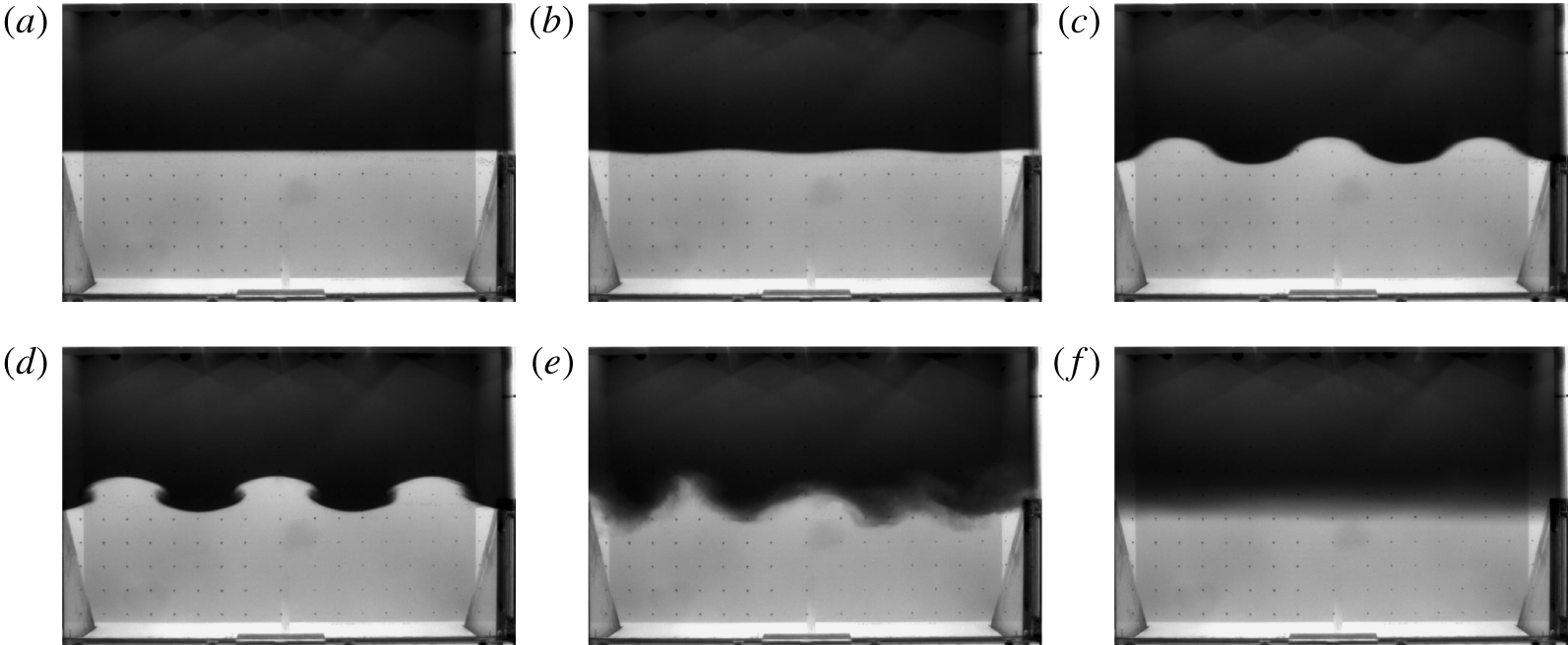
 $8~\text{cm}\leqslant L_{end}\leqslant 40~\text{cm}$. The experimental facility will be described in § 3. A typical time evolution of the interface and mixing zone is shown in figure 1, as seen from a camera attached to the moving platform. Starting from a stable stratification between the fresh water on top of salt water, the interface is only a few mm width. When the vertical oscillations of the platform are activated, a wavy motion appears and the amplitude of the interface deformation
 $\unicode[STIX]{x1D709}$ is rapidly amplified, giving birth to well-defined waves, which themselves develop vortices on the edges. This mushroom shape recalls the observations of Thorpe (Reference Thorpe1968) for interfacial gravity waves, where shear develops at the wave nodes, thus creating some turbulent mixing, and the structures eventually break. After typically two or three minutes of forcing, corresponding roughly to a hundred oscillations, the instability has saturated and the excitation is stopped. The fluid is left to rest and the final mixing zone size
 $L_{end}$ can be measured: because of the small diffusivity of the concentration field (the Schmidt number
 $Sc=\unicode[STIX]{x1D708}/\unicode[STIX]{x1D705}\simeq 700$), this waiting time does not increase artificially
 $L_{end}$.
Snapshots of the experiment Exp A30F3w45 with  $F=0.30$,
 $\unicode[STIX]{x1D714}=4.52~\text{rad}~\text{s}^{-1}$ and
 ${\mathcal{A}}=0.030$ at different times: (a)
 $t=0~\text{s}$; (b)
 $t=46~\text{s}$; (c)
 $t=58~\text{s}$; (d)
 $t=61~\text{s}$; (e)
 $t=111~\text{s}$; (f)
 $t=378~\text{s}$.

The objectives of this work are multiple: (i) To provide an experimental validation of the saturation criterion (1.1), with comparisons with DNS when possible. (ii) To characterise the instability onset, with notably the natural wavelength of the instability and the growth rate of the interface. (iii) To determine the effects of lateral confinement and initial conditions, such as the scale at which perturbations are injected, with the help of DNS. (iv) To predict, thanks to a general theory, the role of the initial mixing layer width on the dynamics.
The paper is organised as follows. Analytical developments are gathered in § 2, where a general approach accounting for the vertical inhomogeneity of the background density profile and viscous dissipation is derived. Then, the experimental apparatus and DNS are detailed in § 3, and difficulties encountered are mentioned. Afterwards, the instability onset and confinement effects are analysed in § 4. Measurements of the final mixing zone size  $L_{end}$ and comparisons with the prediction
 $L_{sat}$ are presented in § 5, along with the time evolution of
 $L(t)$ obtained from DNS and experiments. The existence of a harmonic regime is addressed in § 6. Finally, discussions, perspectives and concluding remarks are gathered in § 7.
2 Equations, modelling and predictions
The purpose of this section is to derive model equations to better understand the dynamics of the turbulent Faraday instability, from onset to saturation. The main theoretical contribution of this work is the approach accounting for the vertical inhomogeneity of the background density profile and viscous dissipation, from which the asymptotic cases of homogeneous stratified turbulence (Gréa & Ebo Adou Reference Gréa and Ebo Adou2018) and interface (Benjamin & Ursell Reference Benjamin and Ursell1954) are recovered. This theory is used to explain and predict some complex features that have been observed experimentally, notably when the instability is triggered from a developed mixing layer.
The incompressible Boussinesq Navier–Stokes and advection equations under periodic and vertical forcing, with  $g(t)=g_{0}(1+F\cos (\unicode[STIX]{x1D714}t))$ along the upward vertical direction
 $\boldsymbol{n}_{\mathbf{3}}$, read in the oscillating tank frame
 $$\begin{eqnarray}\displaystyle & \displaystyle \frac{\unicode[STIX]{x2202}\boldsymbol{U}}{\unicode[STIX]{x2202}t}+(\boldsymbol{U}\boldsymbol{\cdot }\unicode[STIX]{x1D735})\boldsymbol{U}=-\unicode[STIX]{x1D735}P-2{\mathcal{A}}Cg(t)\,\boldsymbol{n}_{\mathbf{3}}+\unicode[STIX]{x1D708}\unicode[STIX]{x1D6FB}^{2}\boldsymbol{U}, & \displaystyle\end{eqnarray}$$
 $$\begin{eqnarray}\displaystyle & \displaystyle \frac{\unicode[STIX]{x2202}C}{\unicode[STIX]{x2202}t}+(\boldsymbol{U}\boldsymbol{\cdot }\unicode[STIX]{x1D735})C=\unicode[STIX]{x1D705}\unicode[STIX]{x1D6FB}^{2}C, & \displaystyle\end{eqnarray}$$
 $$\begin{eqnarray}\displaystyle & \displaystyle \unicode[STIX]{x1D735}\boldsymbol{\cdot }\boldsymbol{U}=0, & \displaystyle\end{eqnarray}$$
 $\boldsymbol{U}$ and
 $C$ are the total velocity and concentration fields,
 $P$ is the reduced pressure,
 $\unicode[STIX]{x1D708}$ is the kinematic viscosity and
 $\unicode[STIX]{x1D705}$ the scalar diffusivity: note that
 $\boldsymbol{U}=\mathbf{0}$ in the absence of the instability. Due to the small density contrast, one can assume a linear dependence of density upon concentration, which means that density fluctuations
 $\unicode[STIX]{x1D70C}^{\prime }$ are linked to the reference density
 $\unicode[STIX]{x1D70C}_{0}=(\unicode[STIX]{x1D70C}_{1}+\unicode[STIX]{x1D70C}_{2})/2$ through
 $$\begin{eqnarray}\frac{\unicode[STIX]{x1D70C}^{\prime }}{\unicode[STIX]{x1D70C}_{0}}=2{\mathcal{A}}\left(C-\frac{1}{2}\right).\end{eqnarray}$$
Hence, one has  $C(\unicode[STIX]{x1D70C}_{1})=1$ for the heavy fluid on the bottom, and
 $C(\unicode[STIX]{x1D70C}_{2})=0$ for the light one on top, with
 $\unicode[STIX]{x1D70C}_{1}=\unicode[STIX]{x1D70C}_{0}(1+{\mathcal{A}})$ and
 $\unicode[STIX]{x1D70C}_{2}=\unicode[STIX]{x1D70C}_{0}(1-{\mathcal{A}})$. The total concentration field is decomposed as
 $C=\langle C\rangle _{H}+c$, where
 $\langle C\rangle _{H}$ is the horizontal average in the two homogeneous directions
 $x$ and
 $y$, and
 $c$ the fluctuation verifying
 $\langle c\rangle _{H}=0$. In the absence of a mean velocity field, one has
 $\boldsymbol{U}=\boldsymbol{u}$, where
 $\boldsymbol{u}$ is the fluctuating velocity, and the equations for the fluctuations read
 $$\begin{eqnarray}\displaystyle & \displaystyle \frac{\unicode[STIX]{x2202}c}{\unicode[STIX]{x2202}t}+u_{j}\frac{\unicode[STIX]{x2202}c}{\unicode[STIX]{x2202}x_{j}}=-u_{3}\frac{\unicode[STIX]{x2202}\langle C\rangle _{H}}{\unicode[STIX]{x2202}x_{3}}+\frac{\unicode[STIX]{x2202}\langle u_{3}c\rangle _{H}}{\unicode[STIX]{x2202}x_{3}}+\unicode[STIX]{x1D705}\unicode[STIX]{x1D6FB}^{2}c, & \displaystyle\end{eqnarray}$$
 $$\begin{eqnarray}\displaystyle & \displaystyle \frac{\unicode[STIX]{x2202}u_{i}}{\unicode[STIX]{x2202}t}+u_{j}\frac{\unicode[STIX]{x2202}u_{i}}{\unicode[STIX]{x2202}x_{j}}=-\frac{\unicode[STIX]{x2202}p}{\unicode[STIX]{x2202}x_{i}}-2{\mathcal{A}}g(t)c\unicode[STIX]{x1D6FF}_{i3}+\frac{\unicode[STIX]{x2202}\langle u_{i}u_{3}\rangle _{H}}{\unicode[STIX]{x2202}x_{3}}+\unicode[STIX]{x1D708}\unicode[STIX]{x1D6FB}^{2}u_{i}, & \displaystyle\end{eqnarray}$$
 $$\begin{eqnarray}\displaystyle & \displaystyle \frac{\unicode[STIX]{x2202}u_{i}}{\unicode[STIX]{x2202}x_{i}}=0. & \displaystyle\end{eqnarray}$$
2.1 Inhomogeneous linear inviscid theory
In the following, we develop a theory accounting for the vertical inhomogeneity in the background density profile connecting two layers of miscible fluids. The objective is to understand the effects of the initial stratification – through an initial mixing zone size  $L_{0}$ – on the triggering and development of the instability. In particular, we are interested here in a piecewise concentration profile, namely constant in the pure fluids and linear in between, which yields for the vertical gradient
 $\unicode[STIX]{x1D6E4}=\unicode[STIX]{x2202}_{z}\langle C\rangle _{H}$, a so-called door function, meaning zero in the pure fluids and constant in the mixing layer: nevertheless, in the inviscid framework, any other profile could be used.
The following developments rely on the early work of Yih (Reference Yih1960). As usual, we discard nonlinear terms, along with diffusion and viscosity: we will come back to the latter in § 2.4. Erasing the pressure from (2.3b), one obtains the two main equations
 $$\begin{eqnarray}\displaystyle & \displaystyle \frac{\unicode[STIX]{x2202}}{\unicode[STIX]{x2202}t}\unicode[STIX]{x1D6FB}^{2}u_{3}=2{\mathcal{A}}g(t)\left(\frac{\unicode[STIX]{x2202}^{2}}{\unicode[STIX]{x2202}z^{2}}-\unicode[STIX]{x1D6FB}^{2}\right)c, & \displaystyle\end{eqnarray}$$
 $$\begin{eqnarray}\displaystyle & \displaystyle \frac{\unicode[STIX]{x2202}c}{\unicode[STIX]{x2202}t}=-u_{3}\unicode[STIX]{x1D6E4}. & \displaystyle\end{eqnarray}$$
 $g(t)=g_{0}$, which is essential for the understanding of the full dynamics. After derivation of (2.4a) and using (2.4b), we expand the vertical velocity as
 $u_{3}(k,z,t)=\unicode[STIX]{x1D719}(z)\exp (\text{i}\boldsymbol{k}\boldsymbol{\cdot }\boldsymbol{x})\exp (\text{i}\unicode[STIX]{x1D6FA}t)$, which yields
 $$\begin{eqnarray}\frac{\unicode[STIX]{x2202}^{2}\unicode[STIX]{x1D719}}{\unicode[STIX]{x2202}z^{2}}-k^{2}\left(1+\frac{2{\mathcal{A}}g_{0}\unicode[STIX]{x1D6E4}}{\unicode[STIX]{x1D6FA}^{2}}\right)\unicode[STIX]{x1D719}=0,\end{eqnarray}$$
where  $k=\sqrt{k_{x}^{2}+k_{y}^{2}}$ is the horizontal wavenumber. Equation (2.5), combined with boundary conditions in
 $z=\pm L_{0}/2$, shows that the characteristic frequency
 $\unicode[STIX]{x1D6FA}$ of the system can only take discrete values
 $\unicode[STIX]{x1D6FA}_{i}$ that depend on the horizontal wavenumber
 $k$, corresponding to the solution
 $\unicode[STIX]{x1D719}_{i}$. In other words, for a given horizontal scale, there is a finite number of admissible vertical modes
 $\unicode[STIX]{x1D719}_{i}$ of corresponding frequencies
 $\unicode[STIX]{x1D6FA}_{i}$.
We now come back to the full case with forcing, and we decompose the vertical velocity on the basis of the  $\unicode[STIX]{x1D719}_{i}$, which are solutions of the stationary problem (2.5), according to
 $$\begin{eqnarray}u_{3}(\boldsymbol{k},z,t)=\mathop{\sum }_{i}A_{i}(k,t)\unicode[STIX]{x1D719}_{i}(k,z)\exp (\text{i}\boldsymbol{k}\boldsymbol{\cdot }\boldsymbol{x})=\hat{u} _{3}(k,z,t)\exp (\text{i}\boldsymbol{k}\boldsymbol{\cdot }\boldsymbol{x}).\end{eqnarray}$$
Using this Fourier decomposition along the horizontal in (2.4a)–(2.4b) provides
 $$\begin{eqnarray}\frac{\unicode[STIX]{x2202}}{\unicode[STIX]{x2202}t}\left(\frac{1}{2{\mathcal{A}}g(t)k^{2}}\frac{\unicode[STIX]{x2202}}{\unicode[STIX]{x2202}t}(\unicode[STIX]{x2202}_{z}^{2}-k^{2})\hat{u} _{3}\right)=-\hat{u} _{3}\unicode[STIX]{x1D6E4}.\end{eqnarray}$$
Injecting further the decomposition (2.6) of  $\hat{u} _{3}$ into (2.7), with the use of
 $(\unicode[STIX]{x2202}_{z}^{2}-k^{2})\unicode[STIX]{x1D719}_{i}=2{\mathcal{A}}g_{0}k^{2}\unicode[STIX]{x1D6E4}\unicode[STIX]{x1D719}_{i}/\unicode[STIX]{x1D6FA}_{i}^{2}$ from (2.5), gives
 $$\begin{eqnarray}\mathop{\sum }_{i}\frac{\unicode[STIX]{x1D719}_{i}}{\unicode[STIX]{x1D6FA}_{i}^{2}}\frac{\unicode[STIX]{x2202}}{\unicode[STIX]{x2202}t}\left(\frac{\unicode[STIX]{x2202}A_{i}/\unicode[STIX]{x2202}t}{1+F\cos (\unicode[STIX]{x1D714}t)}\right)=-\mathop{\sum }_{i}A_{i}\unicode[STIX]{x1D719}_{i}.\end{eqnarray}$$
The last argument comes from the fact that the  $\unicode[STIX]{x1D719}_{i}$ constitute a basis on which the decomposition is unique. Defining the amplitude of the concentration field mode
 $a_{i}$ as
 $\unicode[STIX]{x2202}_{t}a_{i}=-\unicode[STIX]{x1D6E4}A_{i}$ according to (2.4b), one ends up with the main theoretical result of this section
 $$\begin{eqnarray}\frac{\unicode[STIX]{x2202}^{2}a_{i}}{\unicode[STIX]{x2202}t^{2}}+\unicode[STIX]{x1D6FA}_{i}^{2}(1+F\cos (\unicode[STIX]{x1D714}t))a_{i}=0.\end{eqnarray}$$
Hence, the stability of the full inhomogeneous inviscid problem is driven by a set of Mathieu equations of characteristic frequency  $\unicode[STIX]{x1D6FA}_{i}$, determined from the problem without forcing: the well-known stability diagram is addressed later on, and some details about the Floquet analysis of this equation are provided in appendix A, especially regarding the determination of the exponential growth rate of unstable modes as a function of
 $k$.
The final task is to determine the  $\unicode[STIX]{x1D6FA}_{i}$. We have assumed a piecewise background concentration profile, with
 $\unicode[STIX]{x1D6E4}=0$ in the unmixed fluids for
 $L_{0}/2\leqslant |z|\leqslant H/2$, and
 $\unicode[STIX]{x1D6E4}=-N^{2}/2{\mathcal{A}}g_{0}$ for
 $|z|\leqslant L_{0}/2$, where
 $H$ is the height of the domain, and
 $L_{0}$ the width of the mixing layer at a given time. In the upper and lower fluids where the density is constant, one has
 $$\begin{eqnarray}\displaystyle & \displaystyle \unicode[STIX]{x1D719}_{i}\left(z\geqslant \frac{L_{0}}{2}\right)=-u_{top}\frac{\sinh \left(k\left(z-\displaystyle \frac{H}{2}\right)\right)}{\sinh \left(\displaystyle \frac{k}{2}(H-L_{0})\right)},\quad \unicode[STIX]{x1D719}_{i}\left(z\leqslant -\frac{L_{0}}{2}\right)=u_{bot}\frac{\sinh \left(k\left(z+\displaystyle \frac{H}{2}\right)\right)}{\sinh \left(\displaystyle \frac{k}{2}(H-L_{0})\right)}, & \displaystyle \nonumber\\ \displaystyle & & \displaystyle\end{eqnarray}$$
 $$\begin{eqnarray}\displaystyle & \displaystyle \unicode[STIX]{x1D719}_{i}\left(|z|\leqslant \frac{L_{0}}{2}\right)=\frac{u_{top}-u_{bot}}{2\sin (kXL_{0}/2)}\sin (kXz)+\frac{u_{top}+u_{bot}}{2\cos (kXL_{0}/2)}\cos (kXz), & \displaystyle\end{eqnarray}$$
 $u_{top}$ and
 $u_{bot}$ are two constants. Writing
 $X_{i}^{2}=N^{2}/\unicode[STIX]{x1D6FA}_{i}^{2}-1$ and ensuring continuity of
 $\unicode[STIX]{x1D719}_{i}$ and
 $\unicode[STIX]{x2202}_{z}\unicode[STIX]{x1D719}_{i}$ at
 $z=\pm L_{0}/2$ provides the important equations
 $$\begin{eqnarray}\displaystyle & \displaystyle \tan \left(kX_{i}\frac{L_{0}}{2}\right)=-X_{i}\tanh \left(\frac{k}{2}(H-L_{0})\right), & \displaystyle\end{eqnarray}$$
 $$\begin{eqnarray}\displaystyle & \displaystyle \tan \left(kX_{i}\frac{L_{0}}{2}\right)=\frac{1}{X_{i}}\frac{1}{\tanh \left(\displaystyle \frac{k}{2}(H-L_{0})\right)}. & \displaystyle\end{eqnarray}$$
 $\tanh ()$ terms are replaced by
 $1$. The admissible
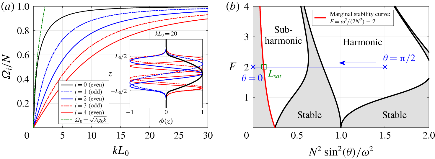
 $\unicode[STIX]{x1D6FA}_{i}$ of the full inhomogeneous problem driven by (2.9) are solutions of the two previous equations, shown in figure 2(a). Solutions of (2.11a) are odd, and of (2.11b) are even. We note that at a given
 $kL_{0}$, several modes
 $\unicode[STIX]{x1D6FA}_{i}$ are excited, which are shown in the inset of figure 2(a). For
 $kL_{0}\gg 1$, the limiting case of homogeneous stratified turbulence is recovered, which corresponds to a fully developed mixing zone with
 $\unicode[STIX]{x1D6FA}_{0}=N$ (Gréa & Ebo Adou Reference Gréa and Ebo Adou2018). On the contrary, for
 $kL_{0}\ll 1$, one has
 $kL_{0}X_{0}/2\simeq 1/X_{0}$, which yields
 $\unicode[STIX]{x1D6FA}_{0}=\sqrt{{\mathcal{A}}g_{0}k}$, which is well recovered in figure 2(a) (green curve) and corresponds to the limiting case of the interface (Benjamin & Ursell Reference Benjamin and Ursell1954).
(a) Characteristic frequency  $\unicode[STIX]{x1D6FA}_{i}$ of the full inhomogeneous problem (2.9) – determined by solving (2.11a)–(2.11b) – normalised by the buoyancy frequency
 $N=(-2{\mathcal{A}}g_{0}\unicode[STIX]{x1D6E4})^{1/2}$, as a function of the horizontal wavenumber
 $k$ and mixing zone extent
 $L_{0}$; inset: vertical profiles
 $\unicode[STIX]{x1D719}_{i}(z)$ at a given
 $kL_{0}$. (b) Stability diagram of (2.12): stability curves (black) separate stable regions (grey) from harmonic and subharmonic unstable regions. An example of the initial condition is displayed in blue, delimited by crosses (from
 $\unicode[STIX]{x1D703}=0$ to
 $\unicode[STIX]{x1D703}=\unicode[STIX]{x03C0}/2$): the square on the marginal stability curve (red) corresponds to the saturation, and the arrow indicates the evolution of
 $N^{2}$ as
 $L$ increases.

The model equation (2.9) is thus used to analyse the turbulent miscible Faraday instability from onset to saturation. Unlike classical linear stability analysis, the interaction between the fluctuating and mean fields is kept, and the reference state given by the characteristic frequency  $\unicode[STIX]{x1D6FA}_{i}$ is updated at each time step since the mixing zone size
 $L$ evolves with time.
2.2 Limiting case of the fully developed mixing zone
In the limiting case of a fully developed mixing zone, the previous general Mathieu equation (2.9) is simplified since all  $\unicode[STIX]{x1D6FA}_{i}$ are constant for
 $kL_{0}\gg 1$. Because of homogeneity, all values of
 $\unicode[STIX]{x1D6FA}_{i}$ between
 $0$ and
 $N=\sqrt{2{\mathcal{A}}g_{0}/L}$ are possible. We thus define
 $\unicode[STIX]{x1D703}_{i}$ as the angle between the wavevector
 $\boldsymbol{k}$ and the vertical axis, so that
 $\tan \unicode[STIX]{x1D703}_{i}=1/X_{i}$, or equivalently
 $\unicode[STIX]{x1D6FA}_{i}=N\sin \unicode[STIX]{x1D703}_{i}$, with notably
 $\unicode[STIX]{x1D6FA}_{0}=N$. For clarity, we write
 $a=a_{i}$ and
 $\unicode[STIX]{x1D703}=\unicode[STIX]{x1D703}_{i}$, which yields the system of equations
 $$\begin{eqnarray}\frac{\unicode[STIX]{x2202}^{2}a}{\unicode[STIX]{x2202}\unicode[STIX]{x1D70F}^{2}}+\frac{N^{2}}{\unicode[STIX]{x1D714}^{2}}\sin ^{2}(\unicode[STIX]{x1D703})(1+F\cos (\unicode[STIX]{x1D70F}))a=0,\end{eqnarray}$$
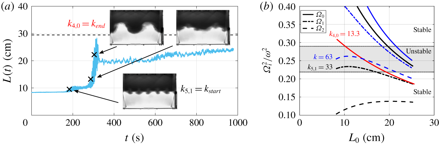
which was first analysed by Gréa & Ebo Adou (Reference Gréa and Ebo Adou2018), where  $\unicode[STIX]{x1D70F}=\unicode[STIX]{x1D714}t$. Such an equation can be solved using Floquet analysis and provides the stability diagram of figure 2(b), where the forcing parameter
 $F$ is a function of the eigenvalues
 $(N\sin \unicode[STIX]{x1D703}/\unicode[STIX]{x1D714})^{2}$. The stability diagram of the general equation (2.9) is the same, except that the eigenvalues are
 $(\unicode[STIX]{x1D6FA}_{i}/\unicode[STIX]{x1D714})^{2}$.
On this diagram, for a given initial condition at a fixed  $F$, many frequencies are excited, corresponding to angles from
 $\unicode[STIX]{x1D703}=0$ to
 $\unicode[STIX]{x1D703}=\unicode[STIX]{x03C0}/2$, which is represented in figure 2(b) by a horizontal segment of extent
 $[0;(N/\unicode[STIX]{x1D714})^{2}]$. If the initial condition
 $(N_{0}/\unicode[STIX]{x1D714})^{2}$ is greater than
 $1/(2F+4)$, then the frequencies beyond the marginal stability curve (red) trigger the instability. As a consequence,
 $L(t)$ grows in size and
 $(N/\unicode[STIX]{x1D714})^{2}$ decreases, which corresponds in figure 2(b) to the right-hand side of the segment going to the left. When it reaches the marginal stability curve, one gets
 $2F+4=\unicode[STIX]{x1D714}^{2}/N_{sat}^{2}$ which eventually yields the saturation criterion (1.1) of Gréa & Ebo Adou (Reference Gréa and Ebo Adou2018). Analytically, the marginal stability curve equation was obtained in the latter reference by performing a multiple time-scale expansion close to the subharmonic resonance
 $N^{2}/\unicode[STIX]{x1D714}^{2}=1/4$. The striking result is that, despite the assumption that
 $F$ is small, the prediction remains quantitatively relevant for larger
 $F$.
2.3 Limiting case of the interface
The opposite limiting case  $kL_{0}\ll 1$ of the general equation (2.9) is the interface for which
 $\unicode[STIX]{x1D6FA}_{0}=\sqrt{{\mathcal{A}}g_{0}k}$, which yields
 $$\begin{eqnarray}\frac{\unicode[STIX]{x2202}^{2}a}{\unicode[STIX]{x2202}\unicode[STIX]{x1D70F}^{2}}+\frac{{\mathcal{A}}g_{0}k}{\unicode[STIX]{x1D714}^{2}}(1+F\cos (\unicode[STIX]{x1D70F}))a=0.\end{eqnarray}$$
Note that this equation is the one derived by Benjamin & Ursell (Reference Benjamin and Ursell1954) for immiscible fluids when setting the surface tension to zero, which was later generalised with viscosity by Kumar & Tuckerman (Reference Kumar and Tuckerman1994). In our experiments, thanks to the large Schmidt number, the interface remains well defined at onset, and has an early time dynamics similar to the immiscible case, as visible in figure 1. This equation (2.13) applies also to the interface position  $\unicode[STIX]{x1D709}$ by noticing that, at first order,
 $\unicode[STIX]{x2202}_{t}\unicode[STIX]{x1D709}=u_{3}$ and
 $\unicode[STIX]{x2202}_{t}c=-\unicode[STIX]{x1D6E4}u_{3}$. Floquet expansion can be used once again to analyse the stability of this equation
 $$\begin{eqnarray}\unicode[STIX]{x1D709}=\frac{1}{2}\text{e}^{\text{i}kx}\text{e}^{(\unicode[STIX]{x1D707}+\text{i}\unicode[STIX]{x1D6FC})\unicode[STIX]{x1D70F}}\mathop{\sum }_{n=-\infty }^{n=+\infty }y_{n}\text{e}^{in\unicode[STIX]{x1D70F}}+\text{cc},\end{eqnarray}$$
where  $\unicode[STIX]{x1D707}+\text{i}\unicode[STIX]{x1D6FC}$ is the Floquet exponent and ‘
 $\text{c.c.}$’ stands for ‘complex conjugate’. The marginal stability curves in figure 2(b) are given by
 $\unicode[STIX]{x1D707}=0$ and delimit the regions of harmonic (
 $\unicode[STIX]{x1D6FC}=0$) and subharmonic (
 $\unicode[STIX]{x1D6FC}=1/2$) instabilities. When
 $\unicode[STIX]{x1D707}\neq 0$, one has access to new tongues located inside the previous ones, corresponding to different growth rates
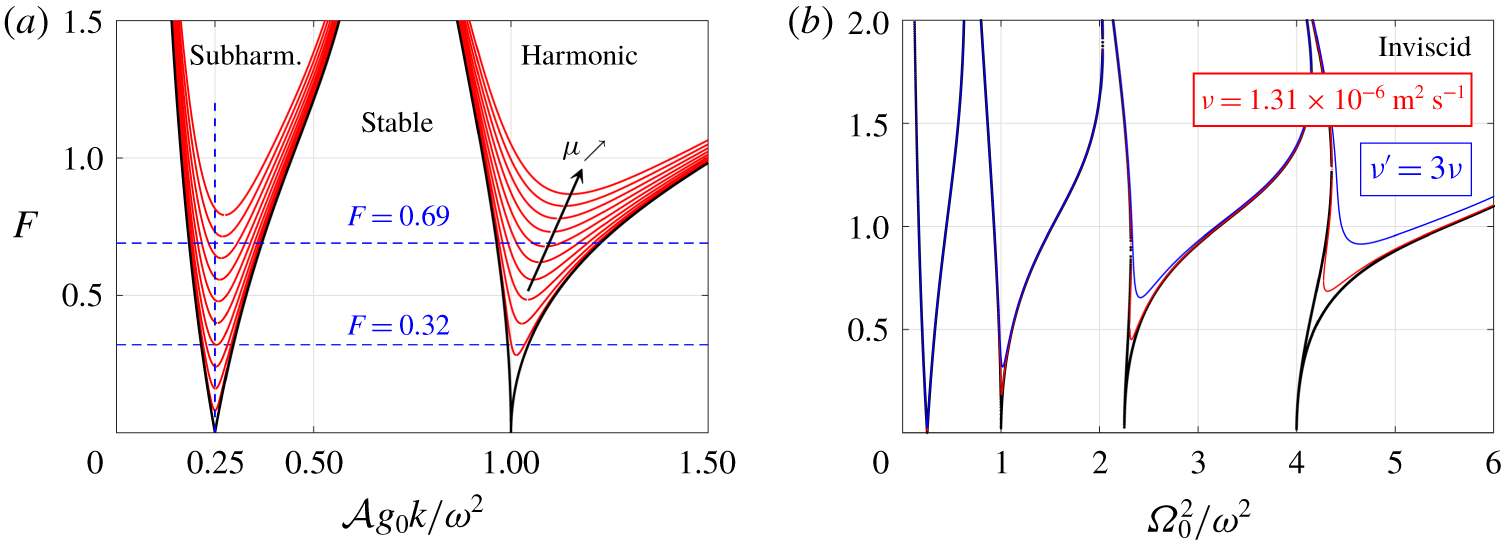
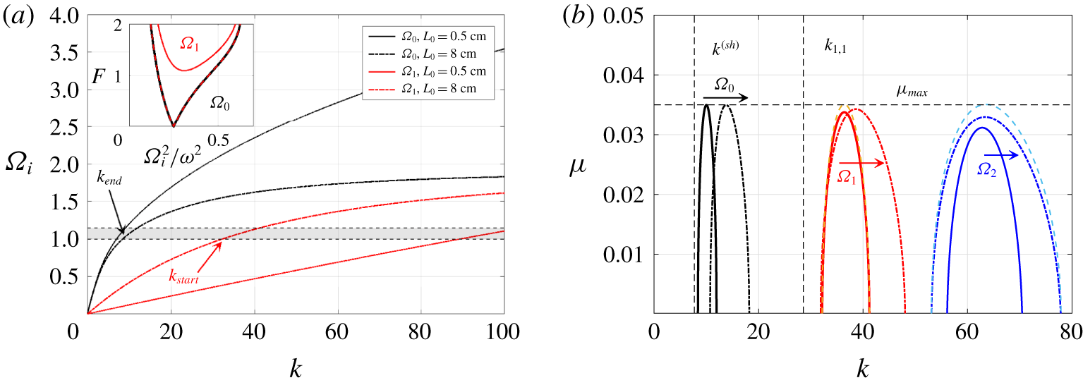
 $\unicode[STIX]{x1D707}$ of unstable modes. These ‘U-tongues’ are presented in figure 3(a) for several values of
 $\unicode[STIX]{x1D707}$. Note that the U-tongues are lifted upwards with increasing
 $\unicode[STIX]{x1D707}$ and their minimum slightly departs from
 $1/4$ in the first subharmonic tongue: this is shown in figure 3(a) with two values of
 $F$. For a given forcing parameter
 $F$ and wavelength
 $\unicode[STIX]{x1D706}=2\unicode[STIX]{x03C0}/k$, this yields the corresponding growth rate of the interface. Consequently, one has, as a first approximation for a subharmonic instability,
 $k^{(sh)}=\unicode[STIX]{x1D714}^{2}/(4{\mathcal{A}}g_{0})$. Hence, the prediction for the wavelength of the most unstable mode starting from an interface, which will be assessed later on, reads
 $$\begin{eqnarray}\unicode[STIX]{x1D706}^{(sh)}=\frac{8\unicode[STIX]{x03C0}{\mathcal{A}}g_{0}}{\unicode[STIX]{x1D714}^{2}}.\end{eqnarray}$$
(a) Stability diagram of (2.13) with the marginal stability curves for  $\unicode[STIX]{x1D707}=0$ (black), and within for various values of the growth rate, from
 $\unicode[STIX]{x1D707}=0.01$ to
 $\unicode[STIX]{x1D707}=0.1$ with a step of
 $0.01$ (red). (b) Stability diagram of the full inhomogeneous viscous problem (2.18) for the mode
 $\unicode[STIX]{x1D6FA}_{0}$ with
 $L_{0}=0.5~\text{cm}$ and three different viscosities, for Exp A15F03w21.

2.4 Inhomogeneous linear viscous theory for piecewise density profile
We conclude our approach dealing with the stability of a mixing zone of arbitrary size  $L_{0}$ by taking into account the effects of viscosity. In order to end up with a rather simple model equation, we still neglect diffusion (
 $\unicode[STIX]{x1D705}=0$) but keep viscous dissipation (
 $\unicode[STIX]{x1D708}\neq 0$), which is consistent with the framework of our experiments where
 $\unicode[STIX]{x1D705}\ll \unicode[STIX]{x1D708}$. Furthermore, unlike the inviscid theory of § 2.1, which applies to any background density profile, we need here to restrict ourselves to a piecewise background density profile for simplicity. Hence, (2.7) is modified into
 $$\begin{eqnarray}\frac{\unicode[STIX]{x2202}}{\unicode[STIX]{x2202}t}\left(\frac{1}{2{\mathcal{A}}g(t)k^{2}}\frac{\unicode[STIX]{x2202}}{\unicode[STIX]{x2202}t}(\unicode[STIX]{x2202}_{z}^{2}-k^{2})\hat{u} _{3}\right)=-\hat{u} _{3}\unicode[STIX]{x1D6E4}+\frac{\unicode[STIX]{x2202}}{\unicode[STIX]{x2202}t}\left(\frac{\unicode[STIX]{x1D708}[\unicode[STIX]{x2202}_{z}^{2}-k^{2}]^{2}\hat{u} _{3}}{2{\mathcal{A}}g(t)k^{2}}\right).\end{eqnarray}$$
Keeping for the vertical velocity the same basis (2.6) of the inviscid case with no forcing tremendously simplifies the problem, since the equations for the amplitude are now decoupled. The full viscous problem, without this convenient basis, was solved by Diwakar et al. (Reference Diwakar, Zoueshtiagh, Amiroudine and Narayanan2015), but does not yield any simple model equation, unlike the present developments. The assumption that  $\unicode[STIX]{x1D6E4}$ is a door function cancels out the
 $\unicode[STIX]{x2202}_{z}^{2}\unicode[STIX]{x1D6E4}$ term when expanding (2.16). One eventually gets
 $$\begin{eqnarray}\frac{\unicode[STIX]{x2202}^{2}a_{i}}{\unicode[STIX]{x2202}\unicode[STIX]{x1D70F}^{2}}-\frac{2{\mathcal{A}}g_{0}\unicode[STIX]{x1D6E4}}{\unicode[STIX]{x1D6FA}_{i}^{2}}\frac{\unicode[STIX]{x1D708}k^{2}}{\unicode[STIX]{x1D714}}\frac{\unicode[STIX]{x2202}a_{i}}{\unicode[STIX]{x2202}\unicode[STIX]{x1D70F}}+\frac{\unicode[STIX]{x1D6FA}_{i}^{2}}{\unicode[STIX]{x1D714}^{2}}(1+F\cos (\unicode[STIX]{x1D70F}))a_{i}=0.\end{eqnarray}$$
In this model equation, the viscous damping term of the miscible Faraday instability depends on several dimensionless quantities: the ratio  $\hat{\unicode[STIX]{x1D6FA}}^{2}=(\unicode[STIX]{x1D6FA}_{i}/\unicode[STIX]{x1D714})^{2}$ between the response frequency and the imposed one, as in the inviscid case; the ratio
 $(N/\unicode[STIX]{x1D6FA}_{i})^{2}$ between the maximum admissible frequency and the response one; and the ratio
 $\unicode[STIX]{x1D708}k^{2}/\unicode[STIX]{x1D714}$ between the characteristic time scale of the forcing and of viscous dissipation. The viscous damping term can be written
 $2\unicode[STIX]{x1D6FE}$ and compared with the phenomenological model proposed in Kumar & Tuckerman (Reference Kumar and Tuckerman1994) (KT) for immiscible fluids, namely
 $2\unicode[STIX]{x1D6FE}_{KT}=4\unicode[STIX]{x1D708}k^{2}$. In our case, taking the interface limit
 $\unicode[STIX]{x1D6FA}_{0}^{2}={\mathcal{A}}g_{0}k$ yields
 $2\unicode[STIX]{x1D6FE}=2k\unicode[STIX]{x1D708}/L_{0}$. The main difference between the present miscible framework and the immiscible one of KT is that the damping
 $\unicode[STIX]{x1D6FE}$ here depends on the width of the diffuse interface
 $L_{0}$. Our model equation also predicts a less intense damping of small scales than in KT, evolving linearly with
 $k$ rather than in
 $k^{2}$.
In addition, it is worth noting that when the mixing zone grows, the damping term  $\unicode[STIX]{x1D6FE}$ decreases. This phenomenology is crucial since it means that viscosity becomes negligible in the homogeneous framework when the mixing layer is fully developed. This justifies a posteriori why the saturation criterion
 $L_{sat}$ of (1.1) is well verified in the DNS of Gréa & Ebo Adou (Reference Gréa and Ebo Adou2018) and Briard et al. (Reference Briard, Gréa and Gostiaux2019) and in the present laboratory experiments.
Equation (2.17) can be simplified using the change of variable  $a_{i}=a_{\unicode[STIX]{x1D708}}\exp (-\unicode[STIX]{x1D6FE}t)$, as in KT, which eventually provides another Mathieu equation
 $$\begin{eqnarray}\frac{\unicode[STIX]{x2202}^{2}a_{\unicode[STIX]{x1D708}}}{\unicode[STIX]{x2202}\unicode[STIX]{x1D70F}^{2}}+\unicode[STIX]{x1D6FA}_{\unicode[STIX]{x1D708}}^{2}(1+F_{\unicode[STIX]{x1D708}}\cos (\unicode[STIX]{x1D70F}))a_{\unicode[STIX]{x1D708}}=0,\end{eqnarray}$$
where  $\unicode[STIX]{x1D6FA}_{\unicode[STIX]{x1D708}}^{2}=\hat{\unicode[STIX]{x1D6FA}}^{2}-\unicode[STIX]{x1D6FE}^{2}/\unicode[STIX]{x1D714}^{2}$ and
 $F_{\unicode[STIX]{x1D708}}=\hat{\unicode[STIX]{x1D6FA}}^{2}F/\unicode[STIX]{x1D6FA}_{\unicode[STIX]{x1D708}}^{2}$. The stability diagram of
 $a_{\unicode[STIX]{x1D708}}$ is the same as in figure 3(a), but with forcing parameter
 $F_{\unicode[STIX]{x1D708}}$ and eigenvalues
 $\unicode[STIX]{x1D6FA}_{\unicode[STIX]{x1D708}}^{2}$. The stability of
 $a_{i}$ is deduced from the one of
 $a_{\unicode[STIX]{x1D708}}$ by determining for each
 $F_{\unicode[STIX]{x1D708}}$ the stability with
 $\unicode[STIX]{x1D707}=\unicode[STIX]{x1D6FE}(k)$ instead, which means that for this problem,
 $F_{\unicode[STIX]{x1D708}}$ is the eigenvalue and
 $\unicode[STIX]{x1D6FA}_{\unicode[STIX]{x1D708}}$ the parameter.
The resulting stability diagram of the full inhomogeneous and viscous problem (2.18) is displayed in figure 3(b) as a function of the true variables  $F$ and
 $(\unicode[STIX]{x1D6FA}_{0}/\unicode[STIX]{x1D714})^{2}$. The diagram is computed for
 $L_{0}=0.5~\text{cm}$ and for the first even mode
 $\unicode[STIX]{x1D6FA}_{0}$: effects of
 $L_{0}$ and
 $\unicode[STIX]{x1D6FA}_{i}$ are discussed later in § 5.2.5. We have chosen the kinematic viscosity of the pure water that is used in our experiments, described in the next section, namely
 $\unicode[STIX]{x1D708}=1.31\times 10^{-6}~\text{m}^{2}~\text{s}^{-1}$, and the configuration Exp A15F3w21 defined later in table 1. We recover, as in the immiscible case (Kumar & Tuckerman Reference Kumar and Tuckerman1994), that viscosity lifts the unstable tongues. But here, the first subharmonic tongue is hardly affected by viscosity, even for
 $\unicode[STIX]{x1D708}^{\prime }=3\unicode[STIX]{x1D708}$, which justifies why hereafter experimental results agree well with the inviscid theory.
Finally, note that the lifting effect of viscosity is much less pronounced for miscible fluids than immiscible ones, because of very different density contrasts. Indeed, for immiscible fluids one has  ${\mathcal{A}}\sim 1$, unlike
 ${\mathcal{A}}=0.015$ here. Moreover, from
 $(\unicode[STIX]{x1D6FA}_{0}/\unicode[STIX]{x1D714})^{2}=0$ to
 $6$, the wavenumber varies from
 $k=0$ to
 $277$, and there are four unstable tongues, which is much less than in KT: hence, a larger Atwood number significantly increases the effects of viscosity.
This approach for the stability and dynamics of a viscous mixing layer between two reservoirs of pure fluids constitutes our main theoretical contribution.
3 Experimental facility and numerical set-up
3.1 The experimental apparatus
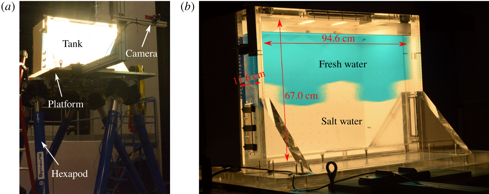
We used an acrylic tank of inner dimensions  $94\times 11\times 67~\text{cm}^{3}$, initially designed for free-surface flow studies at the Gaztransport and Technigaz® (GTT) Motion Analysis and Testing Laboratory.
Fresh water coloured with food dye (Patent Blue V) was first injected in the container, filling half of the volume; then, heavier salt water (using commercial Axal® softening agent consisting of sodium chloride) was injected through a bottom diffuser, very slowly to keep a sharp interface. The density difference between the two fluids ranged between  $10$ and
 $100~\text{kg}~\text{m}^{-3}$ depending on the chosen Atwood number (
 ${\mathcal{A}}=[0.015;0.030;0.045]$), where pure water at
 $20\,^{\circ }\text{C}$ had a constant density of
 $998~\text{kg}~\text{m}^{-3}$. The whole tank was mounted on the platform of a Aquilon model Symétrie® hexapod owned by GTT. The hexapod can induce motions along six axes (translation and rotation), but was only used in this study to generate vertical sinusoidal oscillations, with the acceleration limited to
 $6.87~\text{m}~\text{s}^{-2}$ (corresponding to
 $F=0.70$), the vertical velocity to
 $1.6~\text{m}~\text{s}^{-1}$ and the vertical amplitude to
 $\pm 65~\text{cm}$. A picture of the experimental set-up is visible in figure 4.
(a) Lightened tank on the platform, driven by the six arms of the hexapod. (b) Tank dimensions with  $W=94.6~\text{cm}$,
 $H=67~\text{cm}$ and
 $D=11~\text{cm}$, filled with salt water at the bottom, and fresh water coloured with dye on top of it. Snapshot during the instability.

The platform was initially positioned at  $Z(t=0)=b$. Then, after 20 s of rest, the motion imposed consisted of a series of
 $n$ vertical oscillations
 $Z(t)=b\cos (\unicode[STIX]{x1D714}t)$ starting at
 $t=0~\text{s}$ and ending at
 $2n\unicode[STIX]{x03C0}/\unicode[STIX]{x1D714}$. Here,
 $Z$ refers to the vertical position of the hexapod, which is different from the coordinate
 $z$ in the moving frame. At the end of the oscillation cycle, the platform stood at
 $Z=b$ for 20 s, before being slowly sent back to
 $Z=0$. Note that the choice of a
 $\cos$ function, along with oscillations starting and stopping at
 $Z=b$, ensured that no additional acceleration was introduced at the beginning and at the end of the forcing.
A MicroScale Conductivity and Temperature Instrument (MSCTI) from Precision Measurement Engineering, Inc. was used to measure the density profiles in the tank before and after the experiments. The probe was fixed above the tank, and a slow vertical motion of the hexapod was imposed to obtain a vertical conductivity and temperature profile in the tank. A temperature correction on the conductivity measurements was applied, as the salt water was always cooler than the fresh water, which was slightly heated by the lighting during the slow filling of the tank.
A monochromatic Imaging Development Systems video camera, with a general purpose red gelatine filter in front of the lens, captured, at 45 frames per second, the image of a LED back-lightened white screen as seen through the tank: the resolution of the images is  $856\times 564$ pixels. The camera was attached to the oscillating platform by means of a 1.5 m long Elcom® arm, mechanically reinforced to minimise vibrations. The effect of persistent small vibrations of the camera were further removed during post-processing of the images. Typical raw images of the camera were previously shown in figure 1.
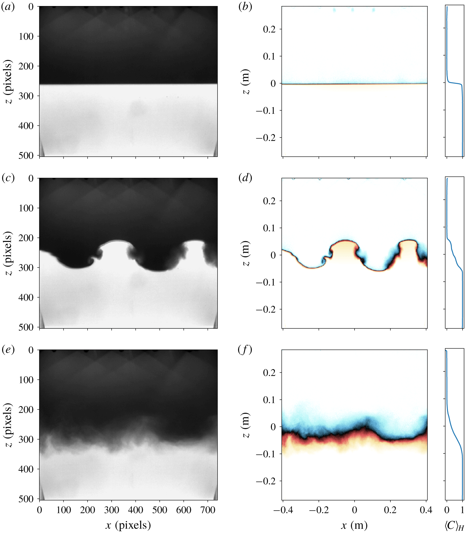
The image intensity was converted into normalised concentration using the Beer–Lambert absorption law for the blue dye. A red gelatine filter was set in front of the camera lens in order to operate in the absorption band of the dye. The aperture and exposure time was optimised so that intensity values covered the 14 bits dynamical range of the camera. The initial concentration field was used to perform a point by point calibration of the intensity accounting for background lighting inhomogeneities. Each image could thus be converted into a depth-averaged and normalised concentration field  $\langle C\rangle _{Y}$, as shown in figure 6 for different stages of the instability. The concentration field obtained was then compared, before and after each experiment, to the measurements of the density probe in order to validate the calibration. It appeared that due to the change in optical index in salt water, the calculation from the camera images slightly under-estimates the instantaneous mixing zone size
 $L(t)$, defined in § 3.3. Therefore, two kinds of results will be proposed: (i)
 $L(t)$ computed from the raw images to investigate the dynamics of the turbulent mixing zone; and (ii)
 $L_{end}$ determined from the conductivity probe to compare with the prediction
 $L_{sat}$.
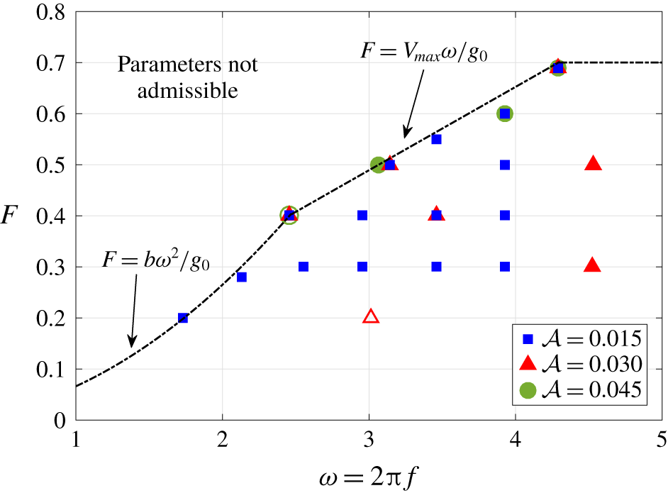
A typical experiment for a given set of parameters lasts approximately for two to three hours, the filling of the tank being obviously the longest part. The tank is washed between each experiment. The authors obtained access for four weeks to GTT and achieved a total of 47 experiments. Various parameters were investigated, as shown in figure 5. Some configurations were repeated several times to check the reproducibility of the results. For the smallest Atwood number  ${\mathcal{A}}=0.015$,
 $\unicode[STIX]{x1D714}$ was varied at constant
 $F$, and on the contrary,
 $F$ was increased at a constant
 $\unicode[STIX]{x1D714}$. A whole region of the parameter map cannot be explored due to the hexapod limitations mentioned earlier.
Map of the configurations explored experimentally. Symbols are for various Atwood numbers:  ${\mathcal{A}}=0.015$ (blue squares),
 ${\mathcal{A}}=0.03$ (red triangles) and
 ${\mathcal{A}}=0.045$ (green circles). One symbol can represent multiple experiments; open symbols mean that the instability was not triggered. The dashed line indicates the boundary of the admissible parameters due to the limitations of the hexapod.

Calibration of the images acquired by the camera for Exp A30F7w43a. (a,c,e): raw images; (b,d,f): calibrated and normalised concentration field, with the mean concentration profile  $\langle C\rangle _{H}(\text{z})$: colour map is yellow for
 $\langle C\rangle _{Y}=1$, light blue for
 $\langle C\rangle _{Y}=0$, black for
 $\langle C\rangle _{Y}=0.5$ and pure fluids are transparent.

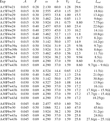
The parameters of the experiments that are discussed in §§ 4–6 are gathered in table 1. Experiments are classified by Atwood number  ${\mathcal{A}}$, then by increasing
 $F$ and finally by increasing
 $\unicode[STIX]{x1D714}$. For all experiments, the initial mixing zone length is evaluated to be approximately
 $0.5~\text{cm}\leqslant L_{0}\leqslant 2.0~\text{cm}$, and depends on the quality of the tank filling. For the final size of the mixing zone
 $L_{end}$, the (p) and (i) mean that it was computed with the probe or the image respectively. The probe measurement is done at one single time, several minutes after the end of the forcing. For (i), we choose a particular image long after the end of the forcing as well.
Parameters of the experiments, sorted by Atwood number  ${\mathcal{A}}$, then by forcing intensity
 $F$ and finally by pulsation
 $\unicode[STIX]{x1D714}\;(\text{rad}~\text{s}^{-1})$. The vertical amplitude
 $b\;(\text{cm})$ and vertical velocity
 $V_{Z}\;(\text{m}~\text{s}^{-1})$ of the platform are given as well, along with the theoretical prediction
 $L_{sat}\;(\text{cm})$ and the measured final size of the mixing zone
 $L_{end}\;(\text{cm})$; (p) means that
 $L_{end}$ was computed with the probe, and (i) with the image.

3.2 The numerical simulations
We have performed direct numerical simulations of the Navier–Stokes–Boussinesq equations (2.1a)–(2.1b) on a triply periodic cubic box of length  $2\unicode[STIX]{x03C0}$, converted into the physical dimensions of the tank
 $W=94.6~\text{cm}$. A classical spectral Fourier collocation method is used with two-third rule dealiasing. The present simulations with
 $1024^{3}$ points are performed using a slab decomposition with 1024 cores. The time increment is determined using a third-order low-storage strong-stability-preserving Runge–Kutta scheme, with implicit viscous terms.
Periodicity in the vertical inhomogeneous direction is ensured by choosing an initial condition in which the concentration field changes sharply from its light to heavy value at the vertical boundaries, as in Briard et al. (Reference Briard, Gréa and Gostiaux2019),
 $$\begin{eqnarray}\displaystyle & \displaystyle C(\boldsymbol{x},t=0)=\frac{1}{2}\left[1+\tanh \left(\frac{z}{\unicode[STIX]{x1D70E}}\right)\right]+C_{inh}(\boldsymbol{x}), & \displaystyle\end{eqnarray}$$
 $$\begin{eqnarray}\displaystyle & \displaystyle C_{inh}(\boldsymbol{x})=-\frac{1}{2}\left[\tanh \left(\frac{z+W/2}{\unicode[STIX]{x1D70E}}\right)+\tanh \left(\frac{z-(W/2-W/N)}{\unicode[STIX]{x1D70E}}\right)\right]. & \displaystyle\end{eqnarray}$$
The first term is the true initial concentration profile, in which the parameter  $\unicode[STIX]{x1D70E}$ is used to modify the initial mixing layer width
 $L_{0}=L(t=0)$. In the present simulations, we set
 $\unicode[STIX]{x1D70E}=0.15~\text{cm}$, so that
 $L_{0}$ is of order
 $1~\text{cm}$. The remaining term
 $C_{inh}$ ensures vertical periodicity at the boundaries. Perturbations of intensity
 $\langle c^{2}\rangle (t=0)/5$, smoothed by a Gaussian filter, are added to this initial concentration profile (3.1). The kinetic energy is initially zero.
Since the term  $C_{inh}$ ensures periodicity in the inhomogeneous vertical direction, a Rayleigh–Taylor instability can be triggered in
 $z=\pm W/2$. A penalisation method is thus implemented to avoid this undesirable phenomenon, and also to mimic the aspect ratio of the GTT tank, with
 $L_{\unicode[STIX]{x1D702}}$ and
 $L_{\unicode[STIX]{x1D702}}^{y}$ the lengths of the penalised domain: more details about the penalisation method can be found in appendix B. We define the height of the penalised box as
 $H=W-L_{\unicode[STIX]{x1D702}}=67~\text{cm}$, and its depth as
 $D=W-L_{\unicode[STIX]{x1D702}}^{y}=11~\text{cm}$. The parameters of the different DNS with
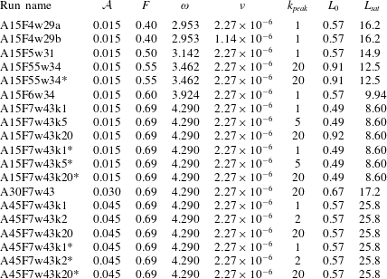
 $1024^{3}$ points, which cover a part of the experiments conducted, are gathered in table 2.
Parameters of the  $1024^{3}$ DNS: Atwood number
 ${\mathcal{A}}$; acceleration ratio
 $F$; pulsation
 $\unicode[STIX]{x1D714}$ (
 $\text{rad}~\text{s}^{-1}$); kinematic viscosity
 $\unicode[STIX]{x1D708}$ (
 $\text{m}^{2}~\text{s}^{-1}$); gravitational acceleration is always
 $g_{0}=9.81~\text{m}~\text{s}^{-2}$; non-dimensional wavenumber
 $k_{peak}$ of the initial scalar variance peak:
 $k_{peak}=20$ means that the initial perturbations’ horizontal length scale is
 $20$ times smaller than the box size
 $W$. The initial scalar variance is always
 $10^{-6}\leqslant \langle c^{2}\rangle \leqslant 10^{-4}$. Initial and predicted final mixing zone sizes
 $L_{0}$ and
 $L_{sat}$ are in cm. The * in some run names means that there is no lateral confinement (
 $L_{\unicode[STIX]{x1D702}}^{y}=0$), and the additional label ‘
 $k$’ specifies the value of
 $k_{peak}$ when necessary.

Finally, there are two main differences between the DNS and the experiments, with important consequences to be underlined. (i) The DNS are periodic along  $x$, and thus, rigid walls of the experiments in the main direction are not taken into account. The consequence of this is visible only for the few configurations that yield experimentally the largest wavelengths, which the DNS cannot reproduce because of periodicity. (ii) The kinematic viscosity is set to
 $\unicode[STIX]{x1D708}=2.27\times 10^{-6}~\text{m}^{2}~\text{s}^{-1}$, which is quite close to the real viscosity of fresh water at
 $20\,^{\circ }\text{C}$, namely
 $1.31\times 10^{-6}~\text{m}^{2}~\text{s}^{-1}$. However, because of our limited spatial resolution, we choose
 $\unicode[STIX]{x1D705}=\unicode[STIX]{x1D708}$ for the diffusivity, whereas in the experiment, the Schmidt number
 $Sc=\unicode[STIX]{x1D708}/\unicode[STIX]{x1D705}$ is of order
 $700$. The impact of such a difference for
 $\unicode[STIX]{x1D705}$ will be seen on the early time evolution of
 $L(t)$. Basically, our too large
 $\unicode[STIX]{x1D705}$ prevents us from investigating small
 $F$ configurations: indeed, in these cases, it requires a long time for the instability to be triggered, time during which the interface diffuses significantly numerically, whereas it remains flat experimentally.
3.3 Computing the mixing zone size  $L(t)$

The mixing layer size  $L(t)$ is a measure of the inner region width between the two pure fluids where there is mixing, and is defined as
 $$\begin{eqnarray}L(t)=K_{L}\int _{fluid}\langle C\rangle _{H}(z)(1-\langle C\rangle _{H}(z))\,\text{d}z,\end{eqnarray}$$
where  $K_{L}=6$ for a linear concentration profile (Gréa Reference Gréa2013). The label ‘fluid’ for the integration domain refers to the vertical length which is not penalised, namely for
 $-H/2\leqslant z\leqslant H/2$. Similarly,
 $\langle C\rangle _{H}$ refers to the horizontal average in the fluid domain,
 $-W/2\leqslant x\leqslant W/2$ and
 $-D/2\leqslant y\leqslant D/2$. The definition (3.3) comes from the turbulent framework of the Rayleigh–Taylor instability (Andrews & Spalding Reference Andrews and Spalding1990) where there are no waves. Here, it also takes into account the deformation of the interface in the early time dynamics even if there is no mixing. Another possibility is to compute profiles of the mixing zone, as
 $$\begin{eqnarray}L_{x}(y,t)=K_{L}\int _{fluid}\langle C\rangle _{X}(y,z,t)(1-\langle C\rangle _{X}(y,z,t))\,\text{d}z,\end{eqnarray}$$
where  $\langle \cdot \rangle _{X}$ unambiguously refers to the average along the homogeneous
 $x$-direction. Then,
 $L(t)$ can be obtained by averaging
 $L_{x}(y,t)$ on the fluid domain along
 $y$, which yields results similar to (3.3): an example is shown in § 4.3.
For the experimental measurements, this is slightly different. The raw images do not contain  $C$, but the depth-averaged concentration field
 $\langle C\rangle _{Y}$. When computing the time evolution of
 $L(t)$, averaging
 $\langle C\rangle _{Y}$ along
 $x$, for each
 $z$, gives
 $\langle C\rangle _{H}(z)$, so that (3.3) can be used. For the probe measurements at the end of the instability, we only get
 $C(z)$ at one position (
 $x$,
 $y$). We nevertheless assume that this measurement is close to
 $\langle C\rangle _{H}(z)$ since we have waited long enough after the end of the forcing so that the stratification is horizontally uniform.
Finally, because of non-uniform lighting, the measure of the pure fluids’ concentrations can slightly differ from  $C=0$ and
 $C=1$ when post-processing the images from the camera. Hence, the constant
 $K_{L}$ of (3.3) is adapted and the integration domain is restricted to values of the concentration between
 $C_{min}=C(z_{min})$ and
 $C_{max}=C(z_{max})$, where
 $\unicode[STIX]{x0394}C=C_{max}-C_{min}$, with the interface at
 $z=0$ so that
 $C(0)=1/2$. Hence, one has
 $K_{L}=12/(\unicode[STIX]{x0394}C(3-\unicode[STIX]{x0394}C^{2}))$. For
 $\unicode[STIX]{x0394}C=1$, one recovers (3.3), and for
 $\unicode[STIX]{x0394}C=0.90$, the value that will be used when computing
 $L$ from the camera images is
 $K_{L}=6.08828$.
4 The onset of instability and confinement effects
Before investigating the turbulent dynamics of the mixing zone and the final saturated state in § 5, we focus in this section on two features. First, the onset of the instability to assess our prediction (2.15) for the wavelength  $\unicode[STIX]{x1D706}^{(sh)}$ of the linearly most amplified mode, and the exponential growth rate of the interface. And secondly, the effect of lateral confinement with DNS to better understand the results that will be presented in § 5.
4.1 The initial wavelength
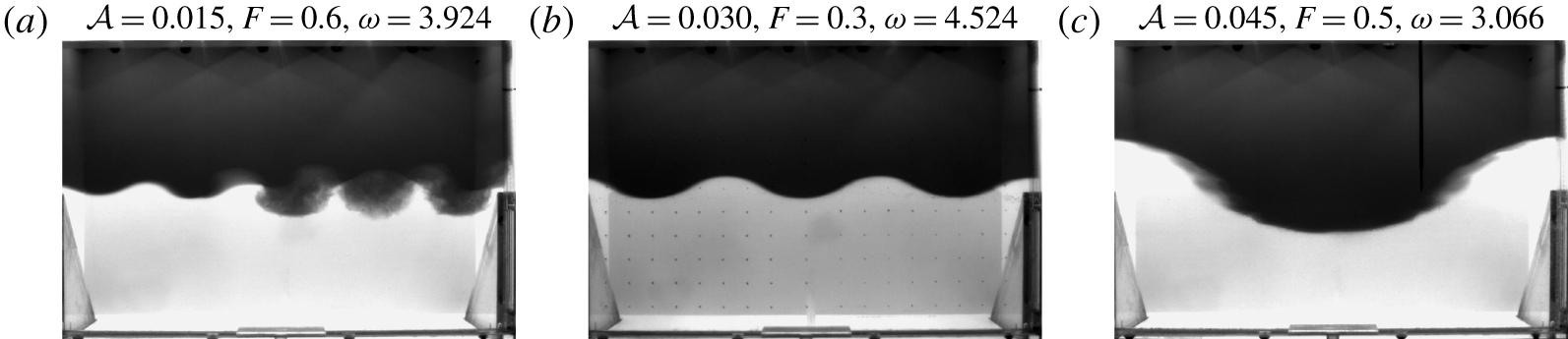
We wish to verify both numerically and experimentally our prediction (2.15) for the wavelength of the initial most amplified mode. To illustrate the variety of wavelengths that have been observed experimentally, raw images of three different experiments are presented in figure 7, for which five, three or only one wavelengths are observed, depending on the control parameters.
Snapshots of (a) Exp A15F6w39 at  $t=32~\text{s}$; (b) Exp A30F3w45 at
 $t=57~\text{s}$; and (c) Exp A45F5w30 at
 $t=60~\text{s}$: a fixed probe was attached to the tank during this experiment.

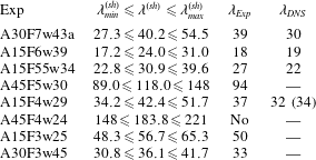
The software ImageJ was used to measure the wavelengths in this kind of raw image, with an error of  $\pm 1~\text{cm}$ for the cases gathered in table 3. For the DNS, the wavelength was determined using Paraview on a vertical slice at the centre of the fluid domain. The prediction
 $\unicode[STIX]{x1D706}^{(sh)}$ is compared in table 3 to the experiments
 $\unicode[STIX]{x1D706}_{Exp}$ for configurations that yield very different wavelengths; some values of
 $\unicode[STIX]{x1D706}_{DNS}$ are shown as well, and the two values
 $\unicode[STIX]{x1D706}_{min}^{(sh)}$ and
 $\unicode[STIX]{x1D706}_{max}^{(sh)}$ correspond to the boundaries of the subharmonic tongue at a given
 $F$.
The overall agreement is satisfactory: experimental results are in good agreement with the prediction (2.15), and interestingly one has  $\unicode[STIX]{x1D706}_{min}^{(sh)}\leqslant \unicode[STIX]{x1D706}_{Exp}\leqslant \unicode[STIX]{x1D706}^{(sh)}$. For the largest wavelengths,
 $\unicode[STIX]{x1D706}_{Exp}$ is closer to
 $\unicode[STIX]{x1D706}_{min}^{(sh)}$ than
 $\unicode[STIX]{x1D706}^{(sh)}$: this is expected, since because of the solid boundaries along
 $x$, the largest wavelengths have to adjust. Consistently, the smaller wavelengths are closer to
 $\unicode[STIX]{x1D706}^{(sh)}$.
Regarding the DNS, the wavelength of the most amplified mode is slightly smaller than in experiments: this might be the consequence of diffusion being greater numerically, possibly the periodicity along  $x$, but also the initial conditions which are obviously different in DNS and experiments. Nevertheless,
 $\unicode[STIX]{x1D706}_{DNS}$ is rather independent of the kinematic viscosity where
 $\unicode[STIX]{x1D708}$ in run A15F4w29b is half as large as run A15F4w29a.
Finally, the instability was not triggered in Exp A45F4w24, because all the admissible wavelengths were much larger than the tank size:  $\unicode[STIX]{x1D706}_{min}^{(sh)}>94.6~\text{cm}$. On the contrary, for Exp A45F5w30, the most amplified wavelength
 $\unicode[STIX]{x1D706}^{(sh)}$ is larger than the tank size, but some of the smallest wavelengths are admissible,
 $\unicode[STIX]{x1D706}_{min}^{(sh)}\leqslant 94.6~\text{cm}$, which explains why the instability was eventually triggered.
Prediction (2.15) for the wavelength  $\unicode[STIX]{x1D706}^{(sh)}$ (in cm) for various configurations sorted by decreasing
 $F$;
 $\unicode[STIX]{x1D706}_{min}^{(sh)}$ and
 $\unicode[STIX]{x1D706}_{max}^{(sh)}$ represent the widths of the first subharmonic tongue at a given
 $F$. Measured values in experiments (with error of order
 $\pm 1~\text{cm}$) and DNS are indicated: the value between parenthesis is for
 $\unicode[STIX]{x1D708}=1.14\times 10^{-6}~\text{m}^{2}~\text{s}^{-1}$.

4.2 The interface growth rate
The aim of this part is to determine the exponential growth rate  $\unicode[STIX]{x1D707}$ of the interface position
 $\unicode[STIX]{x1D709}$ and compare it to the prediction from the Mathieu stability diagram in figure 3(a). We first need to reconstruct the interface from images of the experiments, an idea which is inspired from the work of Jalikop & Juel (Reference Jalikop and Juel2009) for immiscible fluids horizontally accelerated. This analysis is valid when the interface remains well defined, i.e. before wave breaking, and when only one wavelength is unstable: this corresponds to the wave breaking transition to turbulence scenario.
For the sake of reproducibility, we use a simple procedure to detect the interface, detailed in appendix C. Before wave breaking, this reconstructed interface  $\unicode[STIX]{x1D709}_{r}$ at a given time can be approximated by the following analytical fit
 $$\begin{eqnarray}\unicode[STIX]{x1D709}_{r}=a_{0}+a_{1}\cos (kx)+b_{1}\sin (kx),\end{eqnarray}$$
where the amplitudes  $a_{0}$,
 $a_{1}$,
 $b_{1}$ and the wavenumber
 $k$ are the unknowns to be determined. The mean
 $a_{0}$ is very close to
 $0$ initially, and progressively slightly deviates, as shown in appendix C: this artefact reflects the change of optical index in the mixing layer.
In the experiments, because of solid boundaries, a standing wave appears with anti-nodes at the walls. Assuming that only the first subharmonic frequency ( $\unicode[STIX]{x1D6FC}=1/2$) is dominant, the predicted interface can be obtained from (2.14) and reads
 $$\begin{eqnarray}\displaystyle \unicode[STIX]{x1D709}_{f}(x,t) & = & \displaystyle \cos \left(\frac{\unicode[STIX]{x1D714}t}{2}\right)[|y_{0}|\cos (kx+\unicode[STIX]{x1D719}_{0})+|y_{-1}|\cos (kx+\unicode[STIX]{x1D719}_{-1})]e^{\unicode[STIX]{x1D707}\unicode[STIX]{x1D714}t}\nonumber\\ \displaystyle & & \displaystyle +\,\sin \left(\frac{\unicode[STIX]{x1D714}t}{2}\right)[|y_{-1}|\sin (kx+\unicode[STIX]{x1D719}_{-1})-|y_{0}|\sin (kx+\unicode[STIX]{x1D719}_{0})]\text{e}^{\unicode[STIX]{x1D707}\unicode[STIX]{x1D714}t}.\end{eqnarray}$$
We choose the position  $x=0$ at the wall to analyse the time evolution of interface amplitude, which leads to
 $$\begin{eqnarray}\displaystyle \unicode[STIX]{x1D709}_{f}(0,t)=\left[a_{f}\cos \left(\frac{\unicode[STIX]{x1D714}t}{2}\right)+b_{f}\sin \left(\frac{\unicode[STIX]{x1D714}t}{2}\right)\right]\text{e}^{\unicode[STIX]{x1D707}\unicode[STIX]{x1D714}t}=c_{f}\cos \left(\frac{\unicode[STIX]{x1D714}t}{2}+\unicode[STIX]{x1D719}_{f}\right)\text{e}^{\unicode[STIX]{x1D707}\unicode[STIX]{x1D714}t}, & & \displaystyle\end{eqnarray}$$
where  $c_{f}$ and
 $\unicode[STIX]{x1D719}_{f}$ are parameters to be set manually for each configuration to ensure the same phase initially with
 $\unicode[STIX]{x1D709}_{r}$. We now compare the growth rate of the interface amplitude obtained from the experiments with the prediction. We proceed as follows: fitting the images of the interface with (4.1) yields an estimation of the characteristic wavelength
 $2\unicode[STIX]{x03C0}/k$ at onset. This value of
 $k$, along with the control parameters
 $F$,
 $\unicode[STIX]{x1D714}$ and
 ${\mathcal{A}}$, provides a single point in the stability diagram of figure 3(a), and thus yields the predicted Floquet exponent
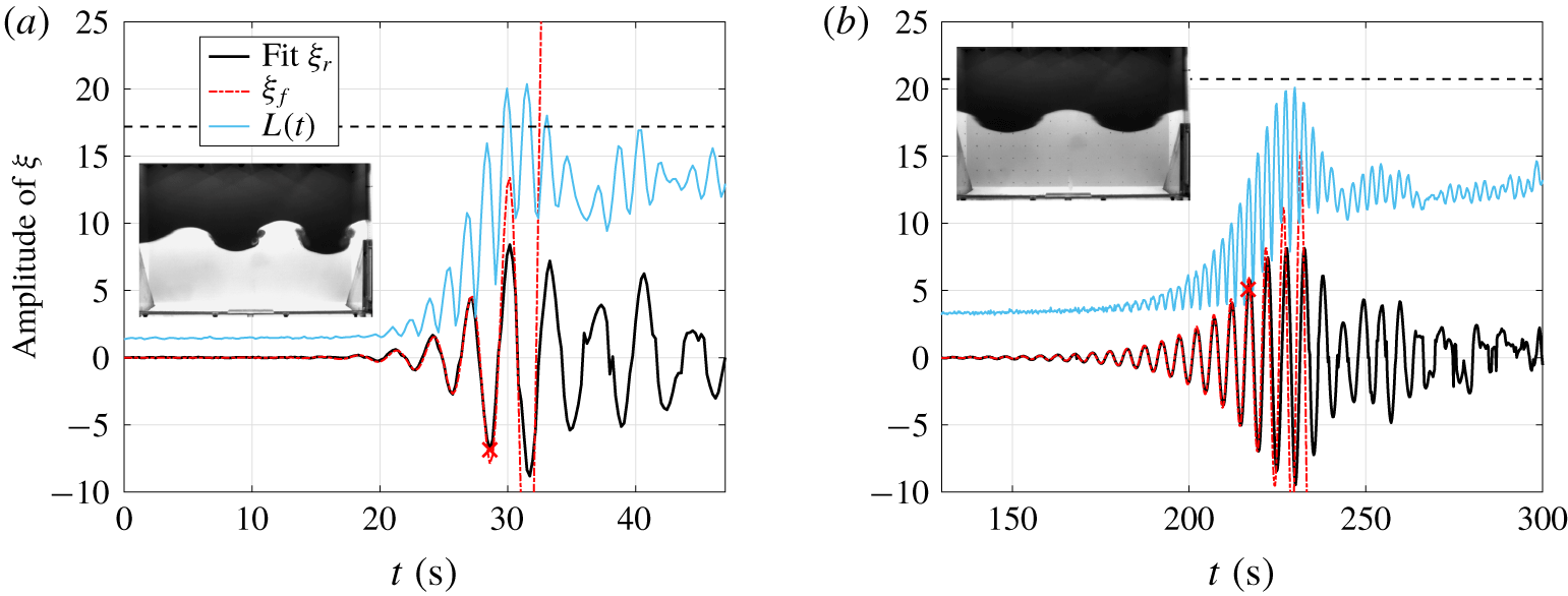
 $\unicode[STIX]{x1D707}$ used in (4.3). Two configurations are shown in figure 8: note that the mixing zone size
 $L(t)$ oscillates twice as fast as the interface, a feature that is expected and explained in § 6.
Amplitude of the reconstructed interface  $\unicode[STIX]{x1D709}_{r}$ (black) along with the prediction
 $\unicode[STIX]{x1D709}_{f}$ (dashed red) and the mixing zone size
 $L(t)$ (blue);
 $L_{sat}$ indicated by a horizontal dashed line. Inset: visualisation of the experiment at the time indicated by a cross. (a) Exp A30F7w43a:
 $\unicode[STIX]{x1D707}=0.0855$ with
 $\unicode[STIX]{x1D706}\simeq 40~\text{cm}$;
 $c_{f}=2.2\times 10^{-4}$ and
 $\unicode[STIX]{x1D719}_{f}=-\unicode[STIX]{x03C0}/2$. (b) Exp A15F3w25:
 $\unicode[STIX]{x1D707}=0.0250$ with
 $\unicode[STIX]{x1D706}\simeq 50~\text{cm}$;
 $c_{f}=5.8\times 10^{-6}$ and
 $\unicode[STIX]{x1D719}_{f}=-\unicode[STIX]{x03C0}/8$.

In figure 8(a) for  $F=0.69$, the instability is triggered rapidly after the activation of the forcing. The fit (4.1) provides
 $\unicode[STIX]{x1D706}\simeq 40~\text{cm}$, close to the prediction, and
 $\unicode[STIX]{x1D707}=0.0855$ using the stability diagram in figure 3(a). The experiment agrees reasonably well with the prediction up to
 $t=28~\text{s}$ (indicated by a cross), thus showing that linear mechanisms dominate the growth of the interface at onset. Then, nonlinearities take the lead when structures break, as shown in the inset of figure 8(a), consistent with
 $L(t)$ becoming much larger and approaching the saturation criterion.
The forcing term is now decreased to  $F=0.3$ and hence it takes much more time for the instability to be triggered in figure 8(b): the other parameters are modified such that the wavelength remains comparable to the previous one, with
 $\unicode[STIX]{x1D706}\simeq 50~\text{cm}$. The exponential growth rate
 $\unicode[STIX]{x1D707}=0.0250$ is more than three times smaller than before and the interface amplitude agrees well with the prediction
 $\unicode[STIX]{x1D709}_{f}$ up to
 $t=216~\text{s}$ (indicated by a cross): at this level, the interface is still well defined as shown by the snapshot. Then,
 $\unicode[STIX]{x1D709}_{r}$ departs from
 $\unicode[STIX]{x1D709}_{f}$, showing the strong effects of nonlinearities. After wave breaking (say for
 $t>230~\text{s}$), there is no more meaning to the ‘interface’: this is also shown in appendix C.
4.3 The effects of confinement in DNS
In this part, we analyse numerically the subtle effect of lateral confinement before investigating the time evolution of  $L(t)$ in the next sections. Two aspects are addressed: the final size of the mixing zone and the onset of instability.
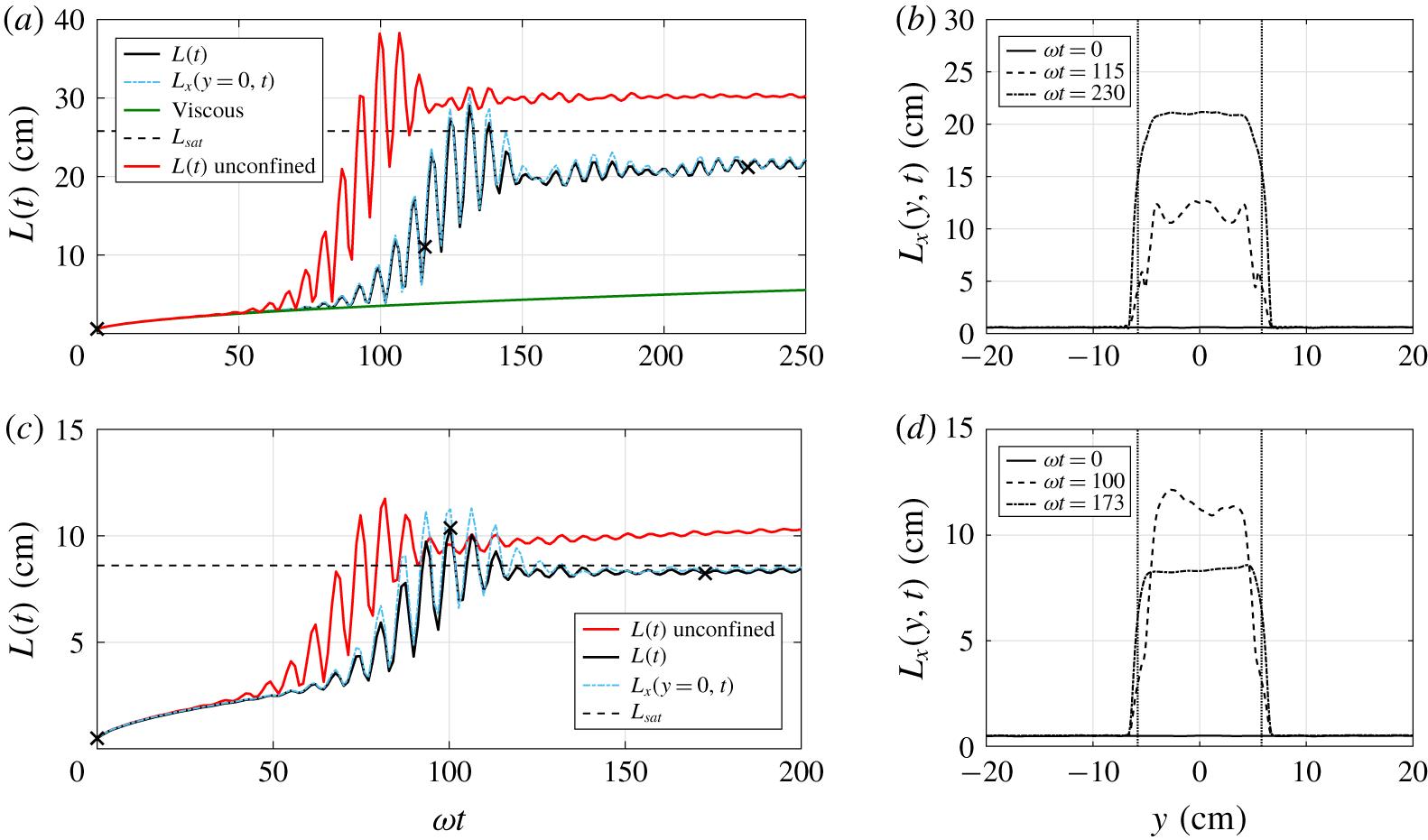
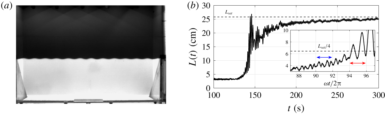
The time evolution of  $L(t)$ in the confined configuration is presented in figure 9(a) for run A45F7w43k20: the initial size is approximately
 $L_{0}\simeq 0.6~\text{cm}$. From approximately
 $\unicode[STIX]{x1D714}t\simeq 60$, the mixing zone starts increasing, and reaches an asymptotic state around
 $\unicode[STIX]{x1D714}t\simeq 150$. Because the forcing is still active, we define the asymptotic state as oscillations of
 $L(t)$ being around a value which does not evolve significantly anymore. Note that the oscillations of
 $L(t)$ are much wider in the subharmonic regime than in the asymptotic state where the instability has saturated.
Profiles of  $L_{x}(y,t)$ in the transverse direction, computed according to (3.4), are given in figure 9(b) for the three different times indicated by crosses in figure 9(a): the fluid domain is located within the vertical dashed lines at
 $y=\pm 5.5~\text{cm}$, from which there are the two penalised regions. One can observe that
 $L_{x}(y,t)$ does not diffuse in the penalised bands thanks to the scalar penalisation, detailed in appendix B.
DNS runs A45F7w43k20 (a,b) and A15F7w43k20 (c,d). (a,c) Time evolution of the averaged mixing zone size  $L(t)$ (black), centred
 $L_{x}(y=0,t)$ (dashed blue) and unconfined (red); the green curve corresponds to the viscous growth; the horizontal dashed line indicates the prediction. (b,d) Profiles of the lateral mixing zone size
 $L_{x}(y,t)$ at three different times indicated by crosses in (a,c); vertical dashed lines represent the limit of the penalised domain.

The dark green curve in figure 9(a) proves that the early growth of the mixing layer is only due to viscous effects with  $L(t)\sim \sqrt{\unicode[STIX]{x1D708}t}$: in practice to obtain this curve,
 $y$ is chosen in a penalised band of an additional simulation without penalisation of the scalar field. The dashed blue curve corresponds to a profile centred in the fluid domain,
 $L_{x}(y=0,t)$, which is by definition different from the depth average that yields
 $L(t)$. The dynamics is nevertheless very similar, with oscillations of slightly larger amplitude. The red curve in figure 9(a) corresponds to run A45F7w43k20*, which is the same as A45F7w43k20 but without any lateral confinement (
 $L_{\unicode[STIX]{x1D702}}^{y}=0$). It appears that with confinement the final mixing zone size
 $L_{end}$ is smaller and that the triggering of the instability is delayed. The decrease of
 $L_{end}$ and delay of onset with lateral confinement are confirmed with runs A15F7w43k20 and A15F7w43k20* in figure 9(c). This configuration is less affected by confinement because the characteristic wavelength
 $\unicode[STIX]{x1D706}^{(sh)}$ is smaller and thus the flow is destabilised in the depth as well: in this case, transition to turbulence is the result of wave interaction.
To better understand the effects of confinement, we performed a detailed analysis in appendix D for the two configurations of figures 9(a) and 9(c), which leads to the following physical interpretation. For a given set of control parameters [ $F$,
 ${\mathcal{A}}$,
 $\unicode[STIX]{x1D714}$], both lateral confinement and the size
 $\unicode[STIX]{x1D706}_{p}$ of the initial perturbations are critical for the early time dynamics. Indeed, confinement reduces the number of modes available for interactions, which slows down nonlinear transfers. But these are responsible for the evolution of
 $\unicode[STIX]{x1D706}_{p}$ towards the natural wavelength of the system: hence, instability is delayed. Furthermore, the energy of the most amplified modes is decreased and the turbulence is damped: hence,
 $L_{end}$ is reduced.
5 The turbulent mixing zone
In the previous section, the theoretical prediction for the wavelength of the most amplified mode has been verified experimentally along with the exponential growth rate of the interface. The effects of confinement were analysed numerically, with the interpretation that nonlinear interactions initially play a role in the time needed to reach the natural frequency of the system and trigger the instability. As an intermediate conclusion, nonlinear transfers are crucial initially – which renders difficult the task of predicting accurately the time at which the instability is triggered – and prevail also when approaching saturation, with wave breaking and irreversible turbulent mixing. Whereas at the onset of the instability, the early time dynamics and growth of the mixing layer are driven by linear production mechanisms.
This section now focuses on the dynamics and saturation of the turbulent mixing zone. We aim at assessing the saturation criterion (1.1) with the experimental measurements of the final size of the mixing layer  $L_{end}$. First, comparisons of
 $L_{end}$ with
 $L_{sat}$ are exposed. Afterwards, time evolutions of
 $L(t)$ obtained from the camera images are presented for some configurations, and compared with DNS. The parameters of the experiments and DNS are given in tables 1 and 2 respectively. For several reasons, such as non-uniform lighting and a slightly moving conductivity probe during the measurements, there is a
 $\pm 1~\text{cm}$ error on the
 $L_{end}$ obtained experimentally.
5.1 The final size of the mixing layer
In this section, we are interested in the final size of the mixing zone  $L_{end}$, which is either determined experimentally or in DNS with the forcing still active in the saturated state. For the experiments,
 $L_{end}$ can be obtained in two different ways: (i) with the conductivity probe after the end of the forcing, whose voltage output signal is corrected to take into account the different temperatures of the fresh and salt water; (ii) with the images of the camera, where the light intensity corresponds to the concentration field, although affected by changes in the optical index in the mixing layer.
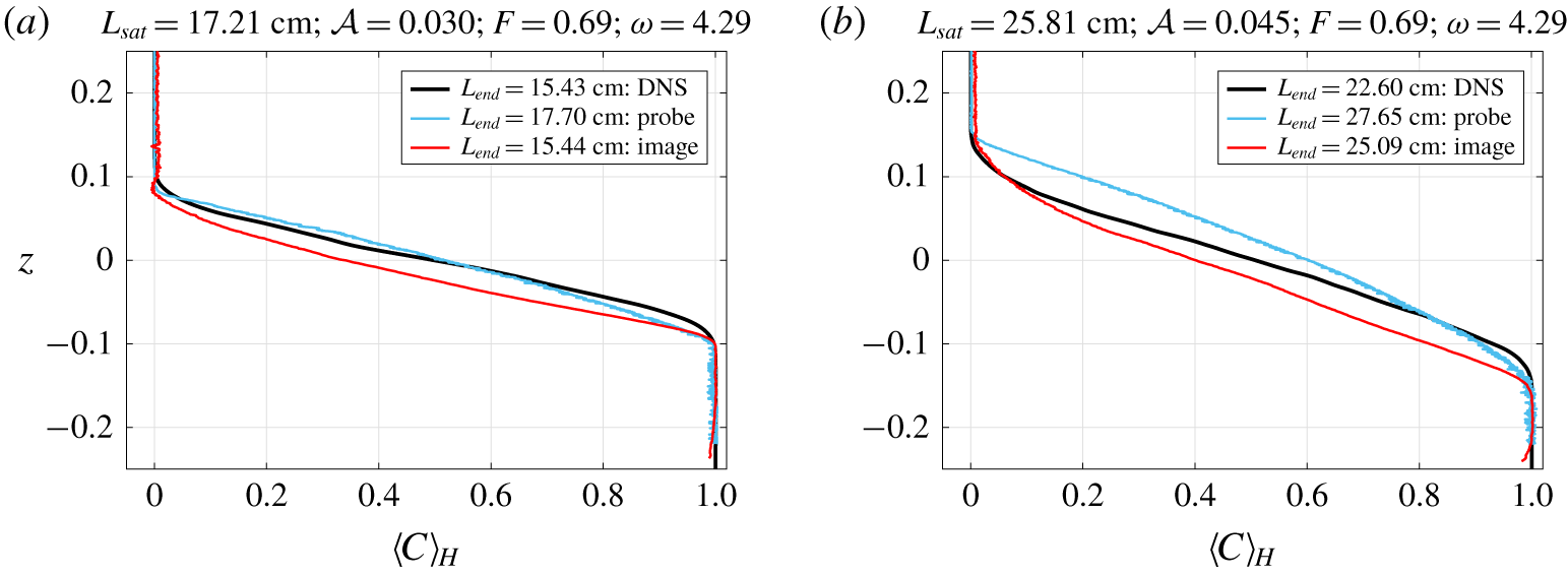
Vertical density profiles of different experimental configurations for  ${\mathcal{A}}=0.030$ and
 ${\mathcal{A}}=0.045$ are presented in figure 10 and are compared with their corresponding DNS. The resulting
 $L_{end}$ is indicated in the legend. There is a good agreement between DNS and experiments for
 $L_{end}$, and further with the prediction
 $L_{sat}$.
Comparison of the mean concentration profile  $\langle C\rangle _{H}$ between DNS and experiments, obtained with the probe and the images for the latter. (a) Exp A30F7w43c with run A30F7w43. (b) Exp A45F7w43b with run A45F7w43k20.

It is worth noting that the experimental profiles  $\langle C\rangle _{H}$, especially with the probe, are sharper near the two pure fluids than the numerical one, because diffusivity is 700 times larger in DNS than in experiments. Moreover, the mean profile in DNS is still affected by the forcing, even though the instability has saturated. It would be too costly numerically to compute a significant duration of physical time with
 $F=0$ after saturation, a time interval in which
 $L(t)$ would also increase due to diffusion.
Note that the computation of  $L_{end}$ with the image (red curves in figure 10) under-estimates the probe value: this is the consequence of the previously mentioned change in optical index, clearly observed by comparing the two experimental profiles
 $\langle C\rangle _{H}$ in figure 10. They agree reasonably well near the pure fluids where the optical index is uniform, and depart from each other in the mixing zone. In fact, the mean concentration profile is shifted downwards with the image. Accordingly, this effect is amplified when the Atwood number increases from
 ${\mathcal{A}}=0.030$ to
 ${\mathcal{A}}=0.045$. Note that the initial level of pure water was modified in Exp A45F7w43b, and this is the reason why
 $\langle C\rangle _{H}(z=0)\neq 1/2$.
Hence, one has to keep in mind that the measurements of  $L_{end}$ with the camera images slightly underestimate the real extent of the mixing layer, approximately by
 $10\,\%$. Nevertheless, when looking at the final sizes
 $L_{end}$ in table 1, they all remain close to the prediction
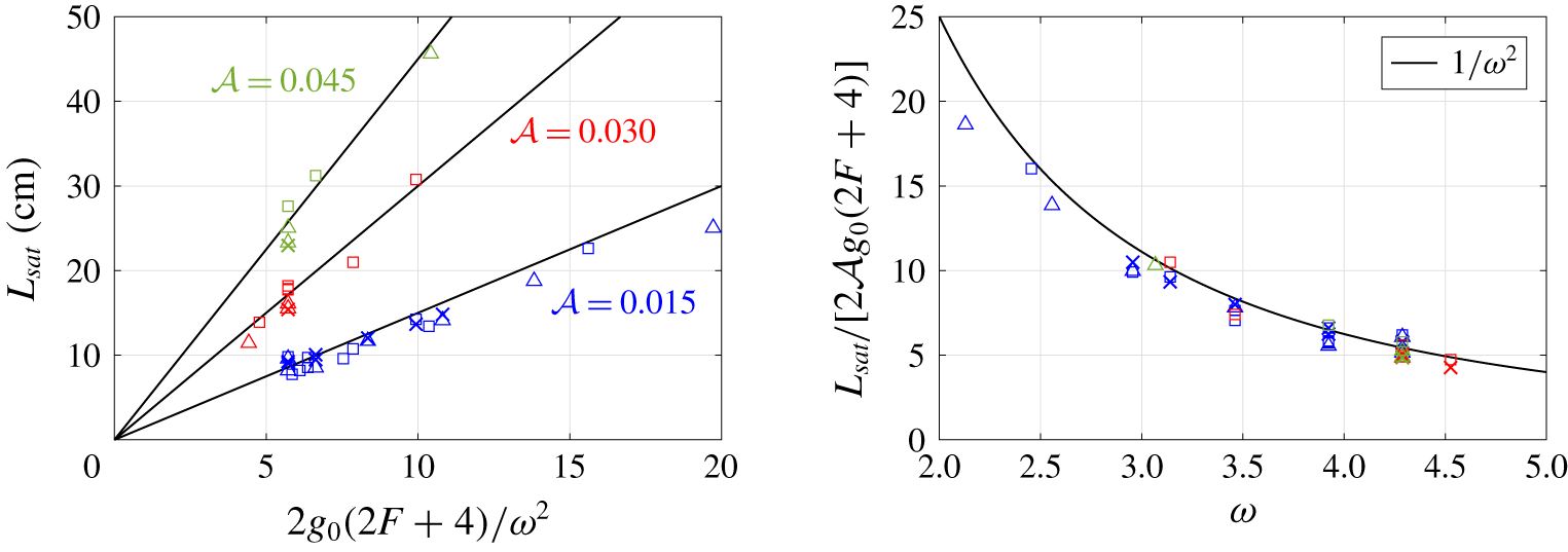
 $L_{sat}$. All these experimental results of table 1 are gathered in figure 11, along with the DNS results of table 2. Two behaviours are verified: on the one hand, the linear dependence in
 ${\mathcal{A}}$, where the prediction
 $L_{sat}$ is plotted as a function of
 $2g_{0}(2F+4)/\unicode[STIX]{x1D714}^{2}$ for the three different Atwood numbers (
 $0.015$ in blue,
 $0.030$ in red and
 $0.045$ in green). On the other hand, the quadratic dependence in
 $\unicode[STIX]{x1D714}$, where
 $L_{sat}/[2{\mathcal{A}}g_{0}(2F+4)]$ is displayed as a function of
 $\unicode[STIX]{x1D714}$. The agreement is convincing enough to assess the prediction, and constitutes the most important contribution of this work.
Comparison between the obtained  $L_{end}$ and the prediction
 $L_{sat}$, for the three Atwood numbers:
 ${\mathcal{A}}=0.015$, blue;
 ${\mathcal{A}}=0.030$, red;
 ${\mathcal{A}}=0.045$, green. Symbols are ▫:
 $L_{end}$ with probe; ▵:
 $L_{end}$ with image; and
 $\times$:
 $L_{end}$ with DNS. (a) The
 ${\mathcal{A}}$-dependence; (b) the
 $\unicode[STIX]{x1D714}$-dependence.

5.2 Time evolution of $L(t)$

In the previous section and in figure 11, it was shown that experimental data agree reasonably well with the saturated mixing layer size prediction for a wide range of parameters. The time evolution of  $L(t)$, obtained experimentally from the images, is now analysed and comparisons with DNS are proposed. In the following subsections, the role of the different control parameters and various observations are discussed in detail, with the emphasis put on the wavelength-selection mechanism when the instability is triggered from a diffuse interface in § 5.2.5.
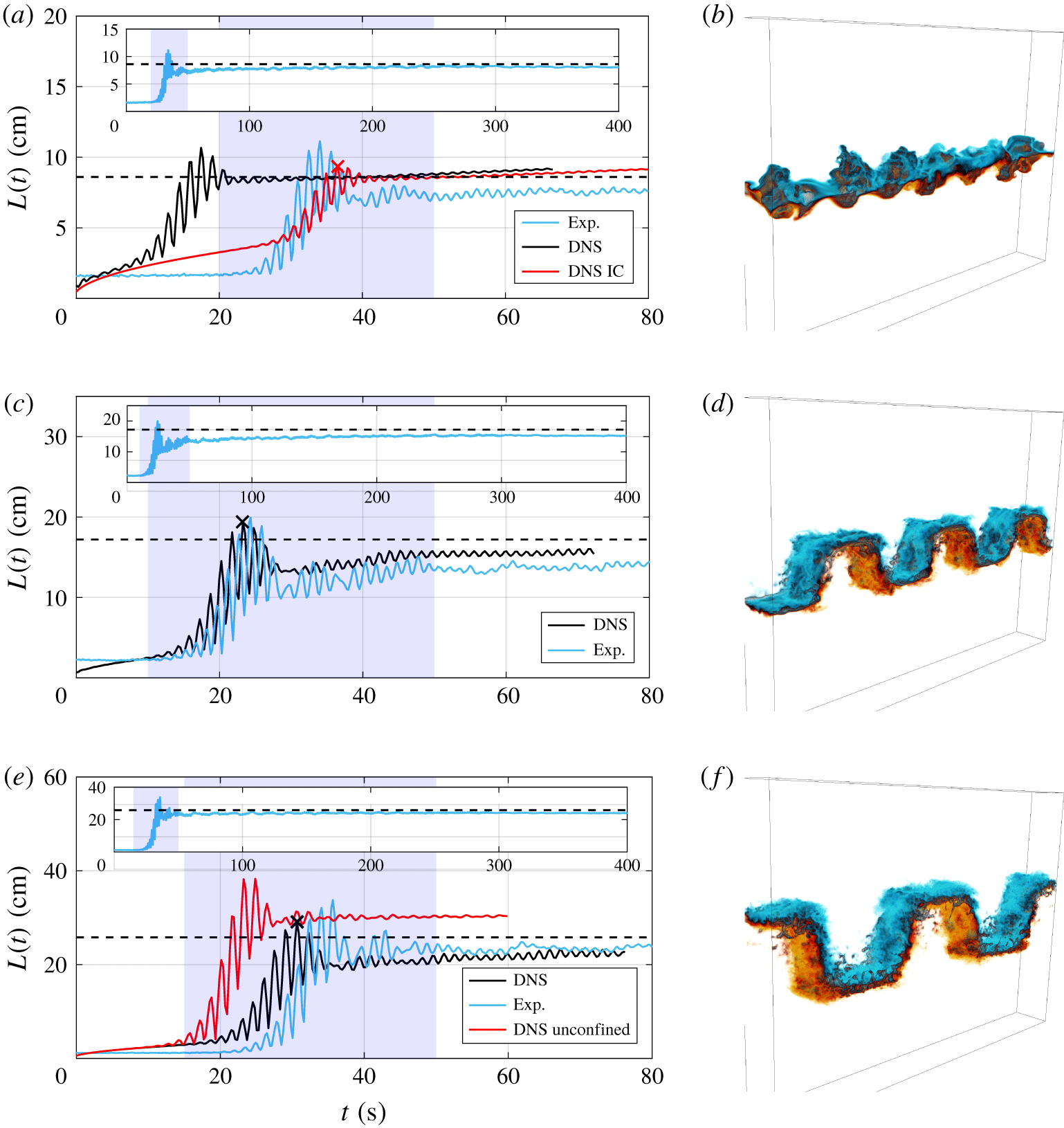
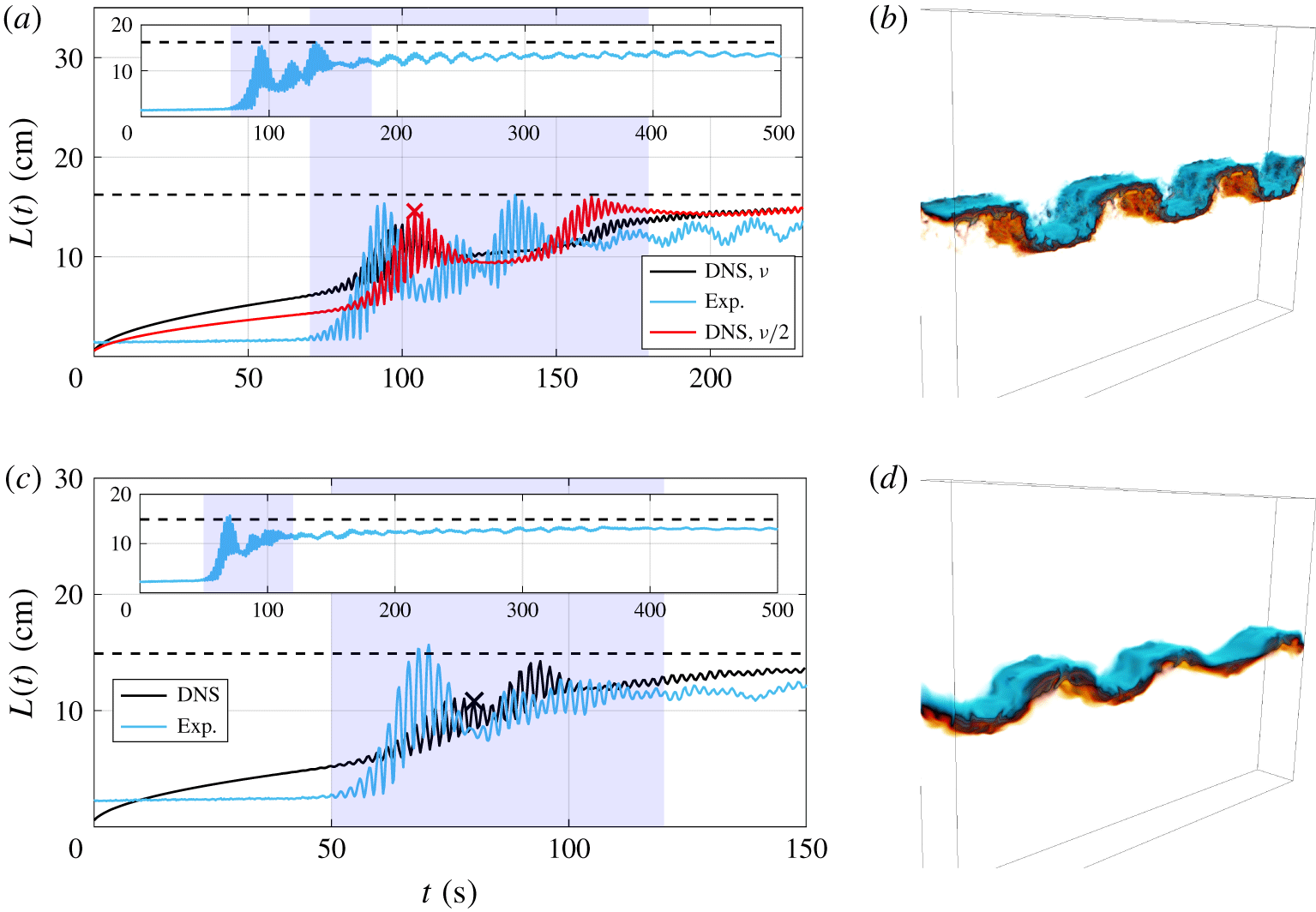
Before moving on, we first make some general observations: figure 12 shows that both numerical and experimental results agree within  $10\,\%$ with the saturation criterion
 $L_{sat}=2{\mathcal{A}}g_{0}(2F+4)/\unicode[STIX]{x1D714}^{2}$. Moreover, for the various configurations presented, the growth of the mixing layer
 $L(t)$ obtained experimentally is in good agreement with the DNS, if some care is given to the initial conditions. One may remark that the overall agreement is better for the most turbulent configurations, namely when the Atwood number is larger.
Note that the forcing is active at  $t=0$ for both the DNS and experiments, and the shaded region corresponds to the time interval where
 $L(t)$ increases significantly during the subharmonic regime and reaches
 $90\,\%$ of
 $L_{end}$.
(a,c,e) Comparison of the time evolution of  $L(t)$ between DNS and experiments, where IC stands for initial conditions;
 $L_{sat}$ is indicated by the horizontal dashed line; the shaded region corresponds to the time interval where
 $L(t)$ increases and reaches
 $90\,\%$ of
 $L_{end}$. (a) Exp A15F7w43a with runs A15F7w43k20 and A15F7w43k1 (red). (c) Exp A30F7w43c with run A30F7w43. (e) Exp A45F7w43a with runs A45F7w43k20 and A45F7w43k20* (red). (b,d,f) Snapshots of runs A15F7w43k1, A30F7w43 and A45F7w43k20, corresponding to the time indicated by a
 $\times$ in (a), (c) and (e) respectively. Colour map: light blue for
 $C=0$, black for
 $C=1/2$ and yellow for
 $C=1$. Pure fluids are transparent to better visualise the mixed fluids.

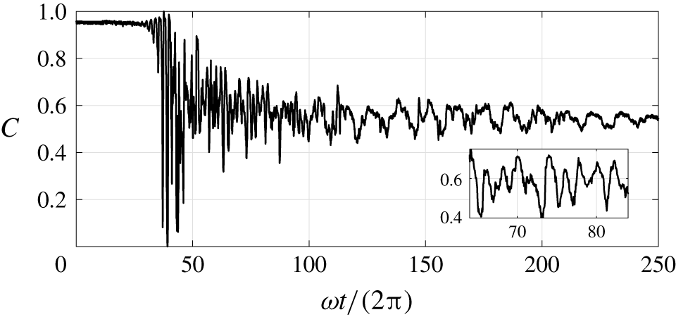
Instantaneous concentration field  $C$ of Exp A45F5w30, as function of
 $\unicode[STIX]{x1D714}t/2\unicode[STIX]{x03C0}$, acquired by the fixed probe shown in figure 7(c).

5.2.1 Impact of the Atwood number
In figure 12, the same forcing parameters are used, namely  $F=0.69$ and
 $\unicode[STIX]{x1D714}=4.29$, and only the Atwood number is increased from
 ${\mathcal{A}}=0.015$ to
 ${\mathcal{A}}=0.045$. Consistently with the prediction (2.15), the wavelength of the most unstable mode increases with
 ${\mathcal{A}}$, as shown in the DNS visualisations of the concentration field in figures 12(b), 12(d) and 12(f). Two different scenarios of transition to turbulence are observed here: wave interaction for
 ${\mathcal{A}}=0.015$ with a transverse mode, and wave breaking for
 ${\mathcal{A}}=0.030$ and
 ${\mathcal{A}}=0.045$, with one single 2-D subharmonic mode (see the raw images of the experiments in supplementary movie 2 for Exp A30F7w43a and movie 3 for Exp A45F7w43a, available at https://doi.org/10.1017/jfm.2019.920)
The final value  $L_{end}$ obtained numerically and experimentally is close to the prediction
 $L_{sat}$ for the three Atwood numbers of figures 12(a), 12(c) and 12(e), within
 $8\,\%$ to
 $10\,\%$. The configuration with
 ${\mathcal{A}}=0.030$ was repeated several times (experiments A30F7w43a, A30F7w43b, A30F7w43c and A30F7w43d), and
 $L_{end}$ measured with the probe remains very similar in table 1,
 $L_{end}=18~\text{cm}\pm 0.3~\text{cm}$, which shows a good reproducibility of the experiments. Consistently with what was underlined previously,
 $L_{end}$ obtained with the images are slightly smaller,
 $15.4~\text{cm}\leqslant L_{end}\leqslant 16.1~\text{cm}$.
In figure 12(a) for  ${\mathcal{A}}=0.015$, the corresponding DNS A15F7w43k20 clearly experiences diffusion effects in the asymptotic state compared to the cases with
 ${\mathcal{A}}=0.030$ and
 ${\mathcal{A}}=0.045$, because the turbulent instability is much less intense: the small oscillations of
 $L(t)$ in the saturated state are smoothed out by diffusion.
5.2.2 The initial condition with $k_{peak}$

The wavelength  $\unicode[STIX]{x1D706}_{p}$ of the initial perturbations is given by
 $k_{peak}$, such that
 $\unicode[STIX]{x1D706}_{p}=W/k_{peak}$. The instability with
 $k_{peak}=20$ (black) for run A15F7w43k20 is triggered long before the experiment in figure 12(a). To better understand this discrepancy, the initial conditions are changed in run A15F7w43k1 (red), while keeping the same control parameters. The concentration variance – whose goal is to disturb the interface – is now localised at large scales with
 $k_{peak}=1$ to better mimic the experiment. For
 $t<20~\text{s}$, the growth of
 $L(t)$ in run A15F7w43k1 is only due to viscous effects, whereas
 $L(t)$ of Exp A15F7w43a remains flat, due to the difference in
 $Sc$. Then, from
 $t\simeq 20~\text{s}$, the instability is triggered in run A15F7w43k1 as in the experiment. Hence, as anticipated, the onset of the instability in DNS depends on the scale at which the concentration variance is injected.
The role of  $k_{peak}$ is essential for run A15F7w43k20 since this configuration is not very turbulent: indeed, the viscous growth of
 $L(t)$ may be dominant initially. This is less the case for runs A30F7w43 and A45F7w43k20 where
 $k_{peak}=20$ with nonetheless a good agreement with experiments: the instability is strong enough to overcome diffusion effects. As discussed in § 4.3 and appendix D, the instability is triggered more rapidly when the size of the initial perturbations, given by
 $k_{peak}$, is close to the most amplified wavelength.
5.2.3 Intermittent asymptotic state
The instantaneous concentration field  $C$ measured with a fixed probe during the experiment is shown in figure 13. The forcing starts when the stronger oscillations appear, around
 $\unicode[STIX]{x1D714}t/(2\unicode[STIX]{x03C0})\simeq 30$. The inset shows a zoom between
 $\unicode[STIX]{x1D714}t/2\unicode[STIX]{x03C0}=70$ and
 $\unicode[STIX]{x1D714}t/2\unicode[STIX]{x03C0}=80$, where there are five periods
 $T$, with
 $T=4\unicode[STIX]{x03C0}/\unicode[STIX]{x1D714}$. Hence, one has
 $C\sim \exp (\text{i}\unicode[STIX]{x1D714}t/2)$ despite a forcing term like
 $\exp (\text{i}\unicode[STIX]{x1D714}t)$, which means that the instability is subharmonic, as expected and already observed in Diwakar et al. (Reference Diwakar, Zoueshtiagh, Amiroudine and Narayanan2015) and Gréa & Ebo Adou (Reference Gréa and Ebo Adou2018).
However, in the asymptotic state with the forcing kept active, one can observe oscillations of large amplitude and small frequency from  $\unicode[STIX]{x1D714}t/2\unicode[STIX]{x03C0}\simeq 120$. This phenomenon was observed in most of the experiments but is hidden when looking at the averaged quantity
 $L(t)$. This is the signature of sweeping by advected fluid at the edges of the mixing layer. Indeed, part of the fluid is not irreversibly mixed due to the weak turbulent diffusion: this effect is obviously more pronounced in the experiments since molecular diffusion is smaller than in DNS.
So, in the experiments we observe locally a decrease of  $L(t)$, thus triggering again locally the instability: fluid is therefore advected elsewhere in the tank, causing the low frequency oscillations seen in figure 13. This phenomenon has also been observed in the rapid acceleration model (Gréa Reference Gréa2013; Gréa & Ebo Adou Reference Gréa and Ebo Adou2018) and could be interpreted as nonlinear interactions between waves and the mixing layer. This mechanism stops when the fluid is at rest after the end of the forcing.
5.2.4 Reynolds number and kinematic viscosity
It is quite complicated to evaluate the Reynolds number in our experiments due to the absence of acquisition systems for the velocity field. Nevertheless, one can estimate it thanks to the associated DNS in the saturated state when the forcing is still active. We define the large-scale Reynolds number as  $Re_{{\mathcal{L}}}=\sqrt{{\mathcal{K}}}{\mathcal{L}}/\unicode[STIX]{x1D708}$, with
 ${\mathcal{K}}$ the kinetic energy and
 ${\mathcal{L}}$ the kinetic energy integral scale. One has for run A45F7w43k20 of figure 12(e) for instance
 $Re_{{\mathcal{L}}}\simeq 500$ in the asymptotic state, and up to
 $Re_{{\mathcal{L}}}^{max}\simeq 2500$ during the instability. For smaller Atwood numbers, like run A15F7w43k20,
 $Re_{{\mathcal{L}}}\simeq 30$, which is consistent with the fact that
 $L(t)$ experiences strong diffusion in the asymptotic state, and
 $Re_{{\mathcal{L}}}\simeq 200$ for run A30F7w43. Obviously, one has
 $Re_{{\mathcal{L}}}=0$ in the asymptotic state of the experiments, after the end of the forcing.
(a,c) Comparison of the time evolution of  $L(t)$ between DNS and experiments;
 $L_{sat}$ is indicated by the horizontal dashed line. (a) Exp A15F4w29 with runs A15F4w29a and A15F4w29b,
 $\unicode[STIX]{x1D708}=2.27\times 10^{-6}~\text{m}^{2}~\text{s}^{-1}$. (c) Exp A15F5w31 with run A15F5w31. (b,d) Screenshots of runs A15F4w29b and A15F5w31, corresponding to the time indicated by a
 $\times$ in (a) and (c) respectively. Colour map as in figure 12.

Regarding the kinematic viscosity, it is recalled that, numerically, we have a unit Schmidt number, meaning  $\unicode[STIX]{x1D708}=\unicode[STIX]{x1D705}$, whereas in experiments
 $Sc\simeq 700$. The effect of decreasing the kinematic viscosity from
 $2.27\times 10^{-6}$ to
 $1.14\times 10^{-6}~\text{m}^{2}$ s
 $^{-1}$ is investigated in figure 14(a) with the two DNS A15F4w29a and A15F4w29b. As expected, the mixing layer grows less initially with
 $\unicode[STIX]{x1D708}=1.14\times 10^{-6}~\text{m}^{2}~\text{s}^{-1}$, and oscillations of
 $L(t)$ are wider, consistent with the flow being more turbulent. As expected for a turbulent flow, the final state given by
 $L_{end}$ is very similar for both viscosities.
Analysis of the change of characteristic wavelength for Exp A15F3w21. (a) Time evolution of the mixing zone, with three snapshots:  $L(t=183~\text{s})=9.5~\text{cm}$,
 $L(t=286~\text{s})=13.3~\text{cm}$,
 $L(t=304~\text{s})=22.2~\text{cm}$. (b) Evolution of the eigenvalues
 $(\unicode[STIX]{x1D6FA}_{i}/\unicode[STIX]{x1D714})^{2}$ of the Mathieu equation (2.9) for the inhomogeneous problem, as a function of
 $L_{0}$ for the three wavenumbers
 $k_{start}=k_{5,1}=33~\text{m}^{-1}$ (black),
 $k_{end}=k_{4,0}=13.3~\text{m}^{-1}$ (red) and
 $k=63~\text{m}^{-1}$ (blue).

5.2.5 Change of characteristic wavelength
Some large amplitude oscillations of  $L(t)$ in the subharmonic regime of experiments A15F4w29 and A15F5w31 can be observed in figures 14(a) and 14(c). They are intrinsically different from those discussed previously in figure 13 which were observed in the asymptotic state.
The present intense oscillations correspond to a change of the characteristic wavelength during the instability. A change of frequency in a diffuse interface between two miscible fluids was also observed by Thorpe (Reference Thorpe1968) in a different framework. Here, there is a first growth of the mixing layer with a given wavelength, then the instability temporarily stops and finally another wavelength is selected as  $L(t)$ grows again. This mechanism of wavelength selection is recovered in DNS A15F4w29a, A15F4w29b and A15F5w31, even though it is blurred by our too large diffusivity. Indeed, in figure 14(a), there are two wide oscillations in DNS against at least three in the experiment.
We aim at understanding this complex phenomenon which seems to occur only for the moderate to small  $F$ configurations: hence, we focus on the experiment A15F3w21 with the smallest forcing parameter,
 $F=0.28$. Because of lateral confinement, one can assume no-slip conditions at the walls, leading to a quantification of the horizontal wavenumber
 $k$. Thus, it can only take the values
 $k_{n,m}=\unicode[STIX]{x03C0}[(n/W)^{2}+(m/D)]^{1/2}$, where
 $D=11~\text{cm}$ and
 $W=94.6~\text{cm}$ are the depth and main size of the tank respectively: notably,
 $k_{1,1}=28.75~\text{m}^{-1}$ is the first admissible 3-D mode. In addition, a particularity of Exp A15F3w21 is that the initial condition consisted of a developed mixing zone rather than a sharp interface: this impacts the early dynamics and will be discussed as well.
The time evolution of  $L(t)$ for Exp A15F3w21 is shown in figure 15(a): at
 $t=183~\text{s}$, one has
 $L\simeq 9.5~\text{cm}$ and five complete wavelengths, namely
 $\unicode[STIX]{x1D706}_{start}\simeq 18.9~\text{cm}$, corresponding to
 $k_{start}=k_{5,1}=33~\text{m}^{-1}$; later, at
 $t=304~\text{s}$, one has
 $L\simeq 22.2~\text{cm}$ with
 $\unicode[STIX]{x1D706}_{end}\simeq 47.3~\text{cm}$ and
 $k_{end}=k_{4,0}=13.3~\text{m}^{-1}$ (the change of wavelength from
 $\unicode[STIX]{x1D706}_{start}$ to
 $\unicode[STIX]{x1D706}_{end}$ can be viewed in supplementary movie 1). As anticipated, none of these wavelengths correspond to the interface prediction
 $\unicode[STIX]{x1D706}^{(sh)}=81.5~\text{cm}$. Given the physical time needed to observe the two wavelengths, the configuration A15F3w21 cannot be investigated properly in DNS, because of the too strong diffusion. Instead, we use the inhomogeneous theory developed in § 2.1 to understand this mechanism.
The stability diagram of the full inhomogeneous equation (2.9) is given in figure 3(b). In figure 15(b), the evolution of the eigenvalue  $(\unicode[STIX]{x1D6FA}_{i}/\unicode[STIX]{x1D714})^{2}$ as a function of the mixing zone size
 $L_{0}$ is presented for the two wavenumbers
 $k_{start}=k_{5,1}$ and
 $k_{end}=k_{4,0}$. The first modes corresponding to frequencies
 $\unicode[STIX]{x1D6FA}_{0}$,
 $\unicode[STIX]{x1D6FA}_{1}$ and
 $\unicode[STIX]{x1D6FA}_{2}$ are displayed, which are the solutions of (2.11a)–(2.11b) shown in figure 2(a). The unstable region represents the width of the subharmonic tongue in figure 3(b) at
 $F=0.28$. Several features should be pointed out:
(a) At onset, for
$L_{0}=8~\text{cm}$, the odd mode with frequency $\unicode[STIX]{x1D6FA}_{1}(k_{start})$ is unstable, and $k_{start}=k_{5,1}$ indicates that the instability is initially three-dimensional, which is confirmed by the pattern in the inset of figure 15(a). Smaller wavelengths are also excited with $\unicode[STIX]{x1D6FA}_{2}(k=63)$ being unstable, which is discussed afterwards.(b) Later, at time
$t=286~\text{s}$, where $L(t)\simeq 13~\text{cm}$, one can observe in the inset of figure 15(a) that two wavelengths coexist, corresponding to two unstable modes: the previous one with frequency $\unicode[STIX]{x1D6FA}_{1}(k_{start})$, and the additional even mode with frequency $\unicode[STIX]{x1D6FA}_{0}(k_{end})$, which is a 2D pattern: with the growth of the mixing zone, a larger wavelength can be sustained.(c) Approaching
$L\simeq 20~\text{cm}$, only $\unicode[STIX]{x1D6FA}_{0}(k_{end})$ is unstable, which is consistent with the large wavelength in figure 15(a). Then, for $L>20~\text{cm}$ and thus much larger times with $t\geqslant 600~\text{s}$, figure 15(b) indicates that $\unicode[STIX]{x1D6FA}_{0}(k_{start})$ is unstable, but very likely at this level many unstable modes of different $k$ contribute to the fully developed mixing layer.


In conclusion, the linear inhomogeneous and viscous theory shows that the spontaneous change of wavelength observed in Exp A15F3w21 is a consequence of both the small forcing parameter – which implies a narrow subharmonic tongue and thus only one unstable mode  $\unicode[STIX]{x1D6FA}_{i}$ at a time – and the initially developed mixing zone which permits selection of multiple wavelengths. This is a wave interaction transition to turbulence scenario, where different subharmonic modes interact with each other within the initial developed mixing layer.
5.2.6 Predicting onset with an initially diffuse interface
In this part, we discuss the ability of our general theory developed in § 2.1 to predict the wavelengths observed when the instability is triggered from a diffuse interface. This is also our opportunity to expose some general results regarding the stability of the modes of frequencies  $\unicode[STIX]{x1D6FA}_{i}$ and the effects of viscosity.
The dependence of the  $\unicode[STIX]{x1D6FA}_{i}$ with the wavenumber
 $k$ for A15F3w21 at
 $F=0.28$ is shown in figure 16(a), and four features should be underlined:
(a) At small
$k$, $\unicode[STIX]{x1D6FA}_{0}$ is much less sensitive to $L_{0}$ than $\unicode[STIX]{x1D6FA}_{1}$: indeed, in the inset of figure 16(a), the two curves $L_{0}=0.5~\text{cm}$ and $L_{0}=8~\text{cm}$ for $\unicode[STIX]{x1D6FA}_{0}$ cannot be distinguished.(b) In the inset,
$\unicode[STIX]{x1D6FA}_{1}$ is quite sensitive to viscosity in the subharmonic tongue for $L_{0}=0.5~\text{cm}$, unlike $\unicode[STIX]{x1D6FA}_{0}$. Increasing $L_{0}$ from $0.5$ to $8~\text{cm}$ for $\unicode[STIX]{x1D6FA}_{1}$ has a similar effect as decreasing viscosity, which is consistent with the expression of the damping term $\unicode[STIX]{x1D6FE}\sim k\unicode[STIX]{x1D708}/L_{0}$.(c) Still, according to the stability diagram in the inset,
$\unicode[STIX]{x1D6FA}_{1}$ would not have been triggered from an interface ($L_{0}\leqslant 0.5~\text{cm}$) for this configuration with $F=0.28$: this is thanks to the initial developed mixing zone such that the instability was triggered with the frequency $\unicode[STIX]{x1D6FA}_{1}(k_{5,1})$.(d) The two curves for
$L_{0}=8~\text{cm}$ reveal that the unstable modes (in the shaded region) for $\unicode[STIX]{x1D6FA}_{1}$ and $\unicode[STIX]{x1D6FA}_{0}$ are precisely the ones observed in figure 15(a), respectively $k_{start}=k_{5,1}$ and $k_{end}=k_{4,0}$. At sufficiently small forcing parameter $F$, these wavenumbers roughly correspond to the characteristic frequency given by $\unicode[STIX]{x1D6FA}_{i}(k)=\unicode[STIX]{x1D714}/2$. Hence, we could have predicted which wavelength would have been triggered from the diffuse interface.


Stability and unstable modes of Exp A15F3w21. (a) Frequencies  $\unicode[STIX]{x1D6FA}_{i}$ as a function of
 $k$ for
 $\unicode[STIX]{x1D6FA}_{0}$ (black) and
 $\unicode[STIX]{x1D6FA}_{1}$ (red), with
 $L_{0}=0.5~\text{cm}$ (–) and
 $L_{0}=8~\text{cm}$ (
 ${-}\,\cdot$), along with the subharmonic unstable region. Inset: first subharmonic tongue of (2.18) with
 $\unicode[STIX]{x1D708}=1.31\times 10^{-6}~\text{m}^{2}~\text{s}^{-1}$. (b) Exponential growth rate
 $\unicode[STIX]{x1D707}$ as a function of
 $k$ for
 $\unicode[STIX]{x1D6FA}_{0}$ (black),
 $\unicode[STIX]{x1D6FA}_{1}$ (red) and
 $\unicode[STIX]{x1D6FA}_{2}$ (blue) at
 $L_{0}=8~\text{cm}$ (–) and
 $L_{0}=15~\text{cm}$ (
 ${-}\,\cdot$): lighter curves (– –) are for the inviscid case at
 $L_{0}=8~\text{cm}$.

The last point to address is why the mode  $\unicode[STIX]{x1D6FA}_{1}(k_{5,1})$ is visible before
 $\unicode[STIX]{x1D6FA}_{0}(k_{4,0})$ in Exp A15F3w21. Although there is no clear answer, we discuss in the following some aspects that provide further insight. The exponential growth rates
 $\unicode[STIX]{x1D707}(k)$ of the unstable modes are displayed in figure 16(b) for
 $\unicode[STIX]{x1D6FA}_{0}$,
 $\unicode[STIX]{x1D6FA}_{1}$ and
 $\unicode[STIX]{x1D6FA}_{2}$ at
 $L_{0}=8~\text{cm}$ and
 $L_{0}=15~\text{cm}$: to compute numerically
 $\unicode[STIX]{x1D707}(k)$, an eigenvalue problem has to be solved, which is detailed in appendix A. First, we recover that the wavenumber
 $k_{max}$ such that
 $\unicode[STIX]{x1D707}(k_{max})=\unicode[STIX]{x1D707}_{max}$ is close to the subharmonic one
 $k^{(sh)}$ for
 $\unicode[STIX]{x1D6FA}_{0}$, and would be even closer at smaller
 $L_{0}$. Then, because of viscosity, the maximum exponential growth rate
 $\unicode[STIX]{x1D707}_{max}$ decreases for
 $\unicode[STIX]{x1D6FA}_{1}$ and
 $\unicode[STIX]{x1D6FA}_{2}$ compared to
 $\unicode[STIX]{x1D6FA}_{0}$. Inviscid curves (– –) are displayed as well for
 $\unicode[STIX]{x1D6FA}_{1}$ and
 $\unicode[STIX]{x1D6FA}_{2}$, proving that, without viscous dissipation,
 $\unicode[STIX]{x1D707}_{max}=0.035$ remains the same for all
 $\unicode[STIX]{x1D6FA}_{i}$ (irrespective of
 $L_{0}$). In addition, when
 $L_{0}$ increases from
 $8$ to
 $15~\text{cm}$, the unstable tongues for
 $\unicode[STIX]{x1D707}$ broaden: the
 $\unicode[STIX]{x1D707}_{max}$ of
 $\unicode[STIX]{x1D6FA}_{1}$ and
 $\unicode[STIX]{x1D6FA}_{2}$ slightly increases as well, because larger
 $L_{0}$ tend to reduce viscous dissipation.
Hence,  $\unicode[STIX]{x1D6FA}_{1}(k_{start})$ is not triggered before
 $\unicode[STIX]{x1D6FA}_{0}(k_{end})$ at
 $L_{0}=8~\text{cm}$ because it has a larger exponential growth rate
 $\unicode[STIX]{x1D707}$. Our interpretation is that, with an initially developed mixing layer, smaller wavelengths can be excited at onset, as confirmed by
 $\unicode[STIX]{x1D6FA}_{2}(k=63)$ being unstable also at
 $L_{0}=8~\text{cm}$ in figure 15(b). Energy is then more easily transferred from
 $\unicode[STIX]{x1D6FA}_{2}(k=63)$ to
 $\unicode[STIX]{x1D6FA}_{1}(k_{start})$.
As a conclusion, the linear inhomogeneous and viscous theory predicts an initial mode competition when the instability is triggered from a diffuse interface, which agrees well with the experiments. We are able to predict which wavelengths may be excited, but the one that is really observed strongly depends on the initial conditions, with very likely a particular sensitivity to  $L_{0}$.
Harmonic regime of Exp A45F7w43b: (a) Stationary state at  $t=110~\text{s}$, which is the end of the initial horizontal forcing of amplitude 5 cm. (b) Time evolution of
 $L(t)$. Inset: zoom at short times of
 $L(t)$ as a function of
 $\unicode[STIX]{x1D714}t/(2\unicode[STIX]{x03C0})$;
 $L_{tr}=L_{sat}/4$ is displayed as a horizontal dashed line.

6 The harmonic regime
The natural configuration of the Faraday instability is a subharmonic regime, where the interface between the two fluids oscillates half as fast as the forcing: this was recovered previously in figure 13, where  $C\sim \exp (\text{i}\unicode[STIX]{x1D714}t/2)$. In terms of the mixing zone, one has
 $L(t)\sim C^{2}\sim \exp (\text{i}\unicode[STIX]{x1D714}t)$, which means that it oscillates as fast as the forcing in the subharmonic regime. This can be clearly seen in figure 8 where
 $L(t)$ oscillates twice as fast as the interface position
 $\unicode[STIX]{x1D709}$.
But some harmonic modes can also be excited initially, as in the example depicted in figure 2(b). In some cases, the harmonic resonances may dominate temporarily: we call this the ‘harmonic regime’ for simplicity, nevertheless keeping in mind that subdominant subharmonic modes are excited as well. We characterise the ‘harmonic to subharmonic transition’ of the instability with the size  $L_{tr}$ from which only subharmonic modes subsist. This transition was numerically analysed in Briard et al. (Reference Briard, Gréa and Gostiaux2019) and can be detected by a change of frequency of the quantity of interest.
The stability diagram of the full inhomogeneous and viscous problem in figure 3(b) shows that  $F$ cannot be too small to observe the harmonic regime, otherwise the first harmonic tongue is not excited. Hence, Exp A45F7w43b was designed to confirm experimentally the existence of the harmonic regime. We created disturbances of an extent that is small compared to the typical subharmonic wavelength of this configuration (
 $\unicode[STIX]{x1D706}^{(sh)}=60~\text{cm}$ from (2.15)) by forcing horizontally the tank during 90 s at
 $\unicode[STIX]{x1D714}$ with an amplitude of
 $5~\text{cm}$. The short wavelength deformation of the interface results from a standing wave that is shown in figure 17(a). When the horizontal forcing is stopped, these deformations decay over a period of ten seconds. Then, the vertical forcing is triggered and, as expected, these small structures are amplified due to the harmonic resonance, before being caught in the more intense subharmonic regime. How can we show this quantitatively?
The time evolution of  $L(t)$ for Exp A45F7w43b is displayed in figure 17(b): the vertical forcing starts at
 $t=120~\text{s}$ (
 $\unicode[STIX]{x1D714}t/2\unicode[STIX]{x03C0}=82$). In the inset, one can observe that, between
 $\unicode[STIX]{x1D714}t/2\unicode[STIX]{x03C0}=94$ and
 $96$, there are two periods, indicated by the double red arrow, assessing the subharmonic regime. Before that, between
 $\unicode[STIX]{x1D714}t/(2\unicode[STIX]{x03C0})=90$ and
 $92$, the frequency is doubled since there are four periods, namely
 $L\sim \exp (2\text{i}\unicode[STIX]{x1D714}t)$. This is precisely the signature of a harmonic regime. As said previously, this is a rather short harmonic regime, visible for ten seconds. The initial size of the mixing zone is
 $L_{0}\simeq 1~\text{cm}$ (measured with the probe) and increases up to approximately
 $3~\text{cm}$ at the end of the initial horizontal forcing. Then, the harmonic regime lasts up to
 $L_{tr}\simeq 6~\text{cm}$ around
 $\unicode[STIX]{x1D714}t/(2\unicode[STIX]{x03C0})=94$. This is consistent with the theory yielding the stability diagram of figure 2(b): the characteristic frequencies in the harmonic and subharmonic regimes are respectively close to
 $(N/\unicode[STIX]{x1D714})^{2}=1$ and
 $(N/\unicode[STIX]{x1D714})^{2}=1/4$, hence there is a ratio of four between
 $L_{tr}$ (at the end of the harmonic regime) and
 $L_{sat}$ (at the end of the subharmonic regime):
 $L_{tr}=L_{sat}/4$ is displayed in the inset of figure 17(b) and indicates quite well the end of the harmonic regime.
The exponential growth rate  $\unicode[STIX]{x1D707}$ of each unstable mode
 $\unicode[STIX]{x1D6FA}_{i}$ as a function of
 $k$ for various
 $L_{0}$ is presented for Exp A45F7w43b in figure 18(a). Unlike figure 16(b) for Exp A15F3w21, the harmonic frequency
 $\unicode[STIX]{x1D6FA}_{0}^{(h)}$ is also unstable at
 $L_{0}=0.5~\text{cm}$, notably because the forcing term is much larger here,
 $F=0.69$: note that its maximum exponential growth rate is smaller than
 $\unicode[STIX]{x1D707}_{max}=0.087$ for
 $\unicode[STIX]{x1D6FA}_{0}^{(sh)}$. When
 $L_{0}$ increases from
 $0.5$ to
 $2~\text{cm}$, the unstable tongues of
 $\unicode[STIX]{x1D6FA}_{0}^{(sh)}$ and
 $\unicode[STIX]{x1D6FA}_{0}^{(h)}$ broaden and move towards larger wavenumbers, unlike
 $\unicode[STIX]{x1D6FA}_{1}^{(sh)}$ which becomes unstable for smaller wavenumbers, with an increasing exponential growth rate: the latter is consistent with the viscous damping decrease for larger mixing layers.
Unstable modes of Exp A45F7w43b: (a) exponential growth rate  $\unicode[STIX]{x1D707}$ as a function of
 $k$ for
 $\unicode[STIX]{x1D6FA}_{0}^{(sh)}$ (black),
 $\unicode[STIX]{x1D6FA}_{0}^{(h)}$ (green) and
 $\unicode[STIX]{x1D6FA}_{1}^{(sh)}$ (red) at
 $L_{0}=0.5~\text{cm}$ (–),
 $L_{0}=1~\text{cm}$ (
 ${-}\,\cdot$),
 $L_{0}=2~\text{cm}$ (– –) and
 $L_{0}=4~\text{cm}$ (
 $\cdots \,$). (b) Evolution of the wavenumber
 $k_{max}$ of the maximum growth rate as a function of
 $L_{0}$ for each
 $\unicode[STIX]{x1D6FA}_{i}$.

The evolution of  $k_{max}$ – defined for each
 $\unicode[STIX]{x1D6FA}_{i}$ as the wavenumber for which the exponential growth rate
 $\unicode[STIX]{x1D707}$ is maximum – as a function of
 $L_{0}$ is presented in figure 18(b). Two outcomes should be underlined:
(a) For both
$\unicode[STIX]{x1D6FA}_{0}^{(sh)}$ and $\unicode[STIX]{x1D6FA}_{0}^{(h)}$, $k_{max}$ increases with larger $L_{0}$ since smaller wavelengths can be excited. When $L_{0}$ significantly departs from the interface limit and reaches a few cm width, there are no more harmonic unstable tongue. This is because, as mentioned previously, harmonic modes quickly saturate, at most when $L_{0}=L_{sat}/4$.(b) For both
$\unicode[STIX]{x1D6FA}_{1}^{(sh)}$ and $\unicode[STIX]{x1D6FA}_{2}^{(sh)}$, $k_{max}$ first decreases before increasing when the mixing layer is sufficiently developed. This is because $\unicode[STIX]{x1D6FA}_{1}^{(sh)}$ and $\unicode[STIX]{x1D6FA}_{2}^{(sh)}$ are strongly affected by viscosity for $L_{0}=0.5~\text{cm}$, and thus can only be destabilised by the largest wavenumbers initially (see for instance figure 16a). On the contrary, when $L_{0}$ increases, the viscous damping is decreased and therefore smaller wavenumbers – still much larger than those for $\unicode[STIX]{x1D6FA}_{0}^{(sh)}$ – can become unstable.


As a conclusion, we have confirmed experimentally the existence of a short harmonic regime, which can only be observed for sufficiently large  $F$ and for a thin enough interface. This harmonic to subharmonic transition of the instability corresponds to a wave interaction transition to turbulence.
7 Conclusions and perspectives
Turbulent mixing triggered by vertical and periodic accelerations was investigated experimentally between fresh and salt water, with the support of direct numerical simulations and theoretical predictions. When the instability is triggered, a natural wavelength appears at the interface between the two fluids. As the amplitude increases, well-defined structures break-up to produce a mixing layer of extent  $L(t)$. Turbulence is eventually inhibited at saturation of the instability, giving a mixing layer of final size
 $L_{end}$.
First, we have developed a new theory accounting for the vertical inhomogeneity of the background density profile and viscous dissipation, notably to predict the onset of the turbulent Faraday instability, either from a sharp or a diffuse interface, and its final saturated state.
At onset of the instability, we have verified experimentally the prediction for the wavelength of the most amplified mode  $\unicode[STIX]{x1D706}^{(sh)}$, and the corresponding exponential growth rate
 $\unicode[STIX]{x1D707}$ of the interface as well. This shows that the early time dynamics of the instability, before wave breaking, is driven by linear mechanisms. The time evolution of the mixing zone
 $L(t)$ and of the interface was obtained after treatment of images captured by the camera: we recovered that the instability was dominated by subharmonic resonances.
With the help of DNS that reproduce the aspect ratio of the tank – but strongly overestimate diffusion due to limited spatial resolution – we have analysed the effects of lateral confinement, which is found to delay the triggering of the instability. Our physical understanding of this phenomenon reads as follows: lateral confinement damps nonlinear interactions, thus slowing down the evolution of the initial perturbations towards the natural wavelength of the instability, and reduces the energy of the most amplified modes. Consequently, when the initial perturbations in the DNS are of the size of the natural wavelength, the instability is triggered much more rapidly.
For some particular initial conditions, we have evidenced a short harmonic response of the instability, by observing an initial frequency doubling of the mixing zone size  $L(t)$, thus confirming recent numerical results (Briard et al. Reference Briard, Gréa and Gostiaux2019). This harmonic regime can only be observed for large enough
 $F$ and small enough
 $L_{0}$.
When the instability is triggered from a diffuse interface rather than a sharp one at small  $F$, experiments have revealed that the characteristic wavelength spontaneously changes. This mode competition can be understood with the inhomogeneous and viscous theory, which permits us to predict the different wavelengths that may develop while the mixing zone grows in size.
Afterwards, we observed two different scenarios for the transition to turbulence: either wave breaking, with only one dominant subharmonic mode from an interface (figure 1), or wave interaction. For the latter, there are three possibilities: the subharmonic mode interacts with a subharmonic mode of the same nature in the transverse direction (figure 7a), with its harmonic mode (figure 17b) or with another subharmonic mode of distinct frequency within the initially developed mixing layer (figure 15a).
Then, in the turbulent regime, the time evolution of the mixing zone  $L(t)$ was compared where possible to DNS, with a good agreement. For the cases of small acceleration ratio
 $F$, we were able to reach very large times in the experiments, which would not have been possible in DNS. At saturation, turbulence is inhibited due to the decrease of the mean concentration gradient. In this asymptotic regime, we observed an intermittent behaviour of the concentration field: due to the large Schmidt number and weak turbulent diffusion, part of the fluid is advected at the edges of the mixing layer, thus possibly triggering again and locally the instability. At the end of the forcing, we used probe measurements to determine the final size of the mixing layer
 $L_{end}$. Our main achievement is the experimental assessment, for a large range of parameters (acceleration, frequency and Atwood number), of the prediction for the final size of the mixing zone at saturation of the instability:
 $L_{sat}=2{\mathcal{A}}g_{0}(2F+4)/\unicode[STIX]{x1D714}^{2}$ (Gréa & Ebo Adou Reference Gréa and Ebo Adou2018).
This study opens the path to mixing layer and instability control in a stratified medium, since the instability could be either activated or inhibited for a given set of control parameters by modifying the initial interface width. Note that similar analytical developments were applied to the case of horizontal vibrations, yielding a different prediction for the final mixing zone size (Gréa & Briard Reference Gréa and Briard2019).
Acknowledgements
DNS were performed at the French computing centre CEA, and received financial support from CEA. Image processing was performed using HPC resources of PMCS2I (École Centrale de Lyon). The authors thank Y. Atik and L. Brosset from the Gaztransport and Technigaz® (GTT) Motion Analysis and Testing Laboratory for accessing the facility and for technical support during the experiments. In addition, the authors would like to thank the referees for their helpful comments.
Declaration of interests
The authors report no conflict of interest.
Supplementary movies
Supplementary movies are available at https://doi.org/10.1017/jfm.2019.920.
Appendix A. Floquet analysis of the model equations
In this appendix, we give some details about the Floquet analysis of the Mathieu equation which is used several times throughout the paper. Following Kumar & Tuckerman (Reference Kumar and Tuckerman1994), the field  $a_{i}$ solution of (2.9), under periodic forcing, can be expanded as
 $$\begin{eqnarray}a_{i}=\text{e}^{(\unicode[STIX]{x1D707}+\text{i}\unicode[STIX]{x1D6FC})\unicode[STIX]{x1D70F}}\mathop{\sum }_{n=-\infty }^{n=+\infty }y_{n}\text{e}^{\text{i}n\unicode[STIX]{x1D70F}},\end{eqnarray}$$
where  $(\unicode[STIX]{x1D707}+\text{i}\unicode[STIX]{x1D6FC})$ is the Floquet exponent. When
 $\unicode[STIX]{x1D707}=0$, the Floquet analysis provides the marginal stability curves of the eigenvalues as a function of the parameter for harmonic (
 $\unicode[STIX]{x1D6FC}=0$) and subharmonic (
 $\unicode[STIX]{x1D6FC}=1/2$) responses. Writing the eigenvalue
 $\hat{\unicode[STIX]{x1D6FA}}^{2}=(\unicode[STIX]{x1D6FA}_{i}/\unicode[STIX]{x1D714})^{2}$, one obtains
 $$\begin{eqnarray}-\frac{1}{\hat{\unicode[STIX]{x1D6FA}}^{2}}([\unicode[STIX]{x1D707}^{2}-(\unicode[STIX]{x1D6FC}+n)^{2}+2\text{i}\unicode[STIX]{x1D707}(\unicode[STIX]{x1D6FC}+n)])y_{n}=y_{n}+\frac{F}{2}(y_{n-1}+y_{n+1}),\end{eqnarray}$$
with for the reality conditions either  $y_{-1}=y_{1}^{\ast }$ for
 $\unicode[STIX]{x1D6FC}=0$, or
 $y_{-1}=y_{0}^{\ast }$ for
 $\unicode[STIX]{x1D6FC}=1/2$. This amounts to solving the generalised eigenvalue problem
 $A_{n}Y_{n}=\hat{\unicode[STIX]{x1D6FA}}^{2}B_{n}Y_{n}$, where
 $F$ is the parameter, and
 $A_{n}$ and
 $B_{n}$ are square matrices of size
 $2(n+1)\times 2(n+1)$: for our purpose,
 $n=8$ is enough and the resolution is performed with MATLAB® using the function eig. Setting
 $\unicode[STIX]{x1D707}=0$ yields the black curves in figure 3(a), and choosing
 $\unicode[STIX]{x1D707}\neq 0$ gives the red ones. This is the classical case, as described in Kumar & Tuckerman (Reference Kumar and Tuckerman1994).
Equation (A 2) can be expressed differently if one is interested in determining for each  $F$ and
 $\hat{\unicode[STIX]{x1D6FA}}^{2}$ the value of the Floquet exponent
 $\unicode[STIX]{x1D707}$. This is a completely different problem, and we consider the inviscid case for simplicity: in practise, we choose one value of
 $F$, corresponding to a given experimental configuration, and set
 $\hat{\unicode[STIX]{x1D6FA}}^{2}$ as the parameter, and thus
 $\unicode[STIX]{x1D707}$ becomes the eigenvalue. But clearly (A 2) provides a quadratic eigenvalue problem that cannot be solved in the same way. A classical way to proceed is to define the variable
 $x_{n}=\unicode[STIX]{x1D707}y_{n}$ so that the quadratic problem is modified into
 $$\begin{eqnarray}[\hat{\unicode[STIX]{x1D6FA}}^{2}-(\unicode[STIX]{x1D6FC}+n)^{2}]y_{n}+\hat{\unicode[STIX]{x1D6FA}}^{2}\frac{F}{2}(y_{n-1}+y_{n+1})+2\text{i}(\unicode[STIX]{x1D6FC}+n)x_{n}=-\unicode[STIX]{x1D707}x_{n},\end{eqnarray}$$
which corresponds to the generalised eigenvalue problem  $\unicode[STIX]{x1D63E}_{n}X_{n}=\unicode[STIX]{x1D707}\unicode[STIX]{x1D63F}_{n}X_{n}$, where
 $\unicode[STIX]{x1D63E}_{n}$ and
 $\unicode[STIX]{x1D63F}_{n}$ are square matrices of size
 $4(n+1)\times 4(n+1)$. In symbolic form, for the harmonic case for example, this gives, with
 $y_{n}=y_{n}^{r}+\text{i}y_{n}^{i}$,
 $$\begin{eqnarray}\displaystyle & & \displaystyle \left(\begin{array}{@{}cccccccccc@{}}\hat{\unicode[STIX]{x1D6FA}}^{2}-n^{2} & 0 & \hat{\unicode[STIX]{x1D6FA}}^{2}F & 0 & \ldots & 0 & -2n & 0 & 0 & \ldots \\ 0 & \hat{\unicode[STIX]{x1D6FA}}^{2}-n^{2} & 0 & 0 & \ldots & 2n & 0 & 0 & 0 & \ldots \\ \hat{\unicode[STIX]{x1D6FA}}^{2}F/2 & 0 & \hat{\unicode[STIX]{x1D6FA}}^{2}-n^{2} & 0 & \ldots & 0 & 0 & 0 & -2n & \ldots \\ 0 & \hat{\unicode[STIX]{x1D6FA}}^{2}F/2 & 0 & \hat{\unicode[STIX]{x1D6FA}}^{2}-n^{2} & \ldots & 0 & 0 & 2n & 0 & \ldots \\ \vdots & \vdots & \vdots & \vdots & \ddots & \vdots & \vdots & \vdots & \vdots & \ddots \\ 0 & 0 & 0 & 0 & \ldots & 1 & 0 & 0 & 0 & \ldots \\ 0 & 0 & 0 & 0 & \ldots & 0 & 1 & 0 & 0 & \ldots \\ 0 & 0 & 0 & 0 & \ldots & 0 & 0 & 1 & 0 & \ldots \\ 0 & 0 & 0 & 0 & \ldots & 0 & 0 & 0 & 1 & \ldots \\ \vdots & \vdots & \vdots & \vdots & \ddots & \vdots & \vdots & \vdots & \vdots & \ddots \end{array}\right)\left(\begin{array}{@{}c@{}}y_{0}^{r}\\ y_{0}^{i}\\ y_{1}^{r}\\ y_{1}^{i}\\ \vdots \\ x_{0}^{r}\\ x_{0}^{i}\\ x_{1}^{r}\\ x_{1}^{i}\\ \vdots \end{array}\right)\nonumber\\ \displaystyle & & \displaystyle \quad =\unicode[STIX]{x1D707}\left(\begin{array}{@{}cccccccccc@{}}0 & 0 & 0 & 0 & \ldots & -1 & 0 & 0 & 0 & \ldots \\ 0 & 0 & 0 & 0 & \ldots & 0 & -1 & 0 & 0 & \ldots \\ 0 & 0 & 0 & 0 & \ldots & 0 & 0 & -1 & 0 & \ldots \\ 0 & 0 & 0 & 0 & \ldots & 0 & 0 & 0 & -1 & \ldots \\ \vdots & \vdots & \vdots & \vdots & \ddots & \vdots & \vdots & \vdots & \vdots & \ddots \\ 1 & 0 & 0 & 0 & \ldots & 0 & 0 & 0 & 0 & \ldots \\ 0 & 1 & 0 & 0 & \ldots & 0 & 0 & 0 & 0 & \ldots \\ 0 & 0 & 1 & 0 & \ldots & 0 & 0 & 0 & 0 & \ldots \\ 0 & 0 & 0 & 1 & \ldots & 0 & 0 & 0 & 0 & \ldots \\ \vdots & \vdots & \vdots & \vdots & \ddots & \vdots & \vdots & \vdots & \vdots & \ddots \end{array}\right)\left(\begin{array}{@{}c@{}}y_{0}^{r}\\ y_{0}^{i}\\ y_{1}^{r}\\ y_{1}^{i}\\ \vdots \\ x_{0}^{r}\\ x_{0}^{i}\\ x_{1}^{r}\\ x_{1}^{i}\\ \vdots \end{array}\right).\end{eqnarray}$$
This change of variable is notably used to obtain figure 16(b).
Appendix B. The penalisation method
In this appendix, we describe the penalisation method implemented in our pseudo-spectral code to mimic ‘solid walls’ and to recover the aspect ratio of the GTT tank. The main dimension along  $x$ is
 $W=94.6~\text{cm}$. The penalisation volume along
 $z$ is of double use: it first reproduces the vertical dimension of the experimental device
 $H=W-L_{\unicode[STIX]{x1D702}}=67~\text{cm}$, and secondly it ensures that no Rayleigh–Taylor instability is triggered due to vertical periodicity. The penalisation volume along
 $y$ reproduces the depth of the tank
 $D=W-L_{\unicode[STIX]{x1D702}}^{y}=11~\text{cm}$.
The penalisation method for the velocity field is inspired from Jause-Labert, Godeferd & Favier (Reference Jause-Labert, Godeferd and Favier2012). Numerically, a term is added to the right-hand side of (2.1a) to mimic a porous medium
 $$\begin{eqnarray}\displaystyle \frac{\unicode[STIX]{x2202}\boldsymbol{U}}{\unicode[STIX]{x2202}t}+(\boldsymbol{U}\boldsymbol{\cdot }\unicode[STIX]{x1D735})\boldsymbol{U}=-\unicode[STIX]{x1D735}P-2{\mathcal{A}}Cg_{0}\,\boldsymbol{n}_{\mathbf{3}}\,(1+F\cos (\unicode[STIX]{x1D714}t))+\unicode[STIX]{x1D708}\unicode[STIX]{x1D6FB}^{2}\boldsymbol{U}-\frac{1}{\unicode[STIX]{x1D702}}\unicode[STIX]{x1D712}\boldsymbol{U}, & & \displaystyle\end{eqnarray}$$
where  $\unicode[STIX]{x1D702}$ is the penalisation parameter and
 $\unicode[STIX]{x1D712}$ the mask function. The penalisation parameter is set to
 $\unicode[STIX]{x1D702}=5\times 10^{-3}$ for an explicit time-integration scheme: varying
 $\unicode[STIX]{x1D702}$ from
 $5.10^{-3}$ to
 $10^{-3}$ does not modify the results. The penalisation mask
 $\unicode[STIX]{x1D712}$ is here a door function
 $D(\boldsymbol{x})$, equal to
 $1$ in the ‘solid’ domain and
 $0$ in the fluid one. To avoid Gibbs oscillations, the mask is further filtered in spectral space using
 $\unicode[STIX]{x1D712}(\boldsymbol{k})=\hat{D}(\boldsymbol{k})\exp (-C_{\unicode[STIX]{x1D702}}(k/N_{p})^{2})$, with
 $N_{p}=1024$ the number of points in one direction, and
 $C_{\unicode[STIX]{x1D702}}=256$ to both preserve the shape and intensity of the mask.
The novelty compared to Briard et al. (Reference Briard, Gréa and Gostiaux2019) is that the concentration field is penalised as well, using the methodology proposed in Kadoch et al. (Reference Kadoch, Kolomenskiy, Angot and Schneider2012): this is essential here given the small depth of the tank. The mask is the same for the two field  $\boldsymbol{U}$ and
 $C$, but the scalar penalisation parameter
 $\unicode[STIX]{x1D702}_{c}$ is now interpreted as an effective diffusivity in the ‘solid’ domain. Numerically, the advection equation (2.1b) is modified into
 $$\begin{eqnarray}\displaystyle \frac{\unicode[STIX]{x2202}C}{\unicode[STIX]{x2202}t}+((1-\unicode[STIX]{x1D712})\boldsymbol{U}\boldsymbol{\cdot }\unicode[STIX]{x1D735})C & = & \displaystyle \unicode[STIX]{x1D735}\boldsymbol{\cdot }((\unicode[STIX]{x1D705}(1-\unicode[STIX]{x1D712})+\unicode[STIX]{x1D702}_{c}\unicode[STIX]{x1D712})\unicode[STIX]{x1D735}C),\end{eqnarray}$$
 $$\begin{eqnarray}\displaystyle & = & \displaystyle \unicode[STIX]{x1D705}\unicode[STIX]{x1D6FB}^{2}C+(\unicode[STIX]{x1D702}_{c}-\unicode[STIX]{x1D705})\unicode[STIX]{x1D735}\boldsymbol{\cdot }(\unicode[STIX]{x1D712}\unicode[STIX]{x1D735}C).\end{eqnarray}$$
Unlike  $\unicode[STIX]{x1D702}$,
 $\unicode[STIX]{x1D702}_{c}$ does not impose any constraint on the time step and can thus be chosen as small as necessary: here we choose
 $\unicode[STIX]{x1D702}_{c}=10^{-7}$. The viscous growth of
 $L(t)$ for run A45F7w43k20 in figure 9(a) was obtained with a simulation without scalar penalisation.
Appendix C. Detection of the interface
In this appendix, we briefly give technical details about the simple method we use to reconstruct the interface in § 4.2 and to determine the coefficients of the analytical fit (4.1). We use the optimised fitting tool of MATLAB called fourier1, which amounts to a decomposition in Fourier modes truncated at the first order using nonlinear least-squares methods. The different steps are illustrated on the case shown in inset of figure 8(b), namely Exp A15F3w25 at  $t=216~\text{s}$.
The image is first centred properly, and the mean intensity captured by the camera is used to make the image black or white without shades of grey, as in figure 19(a). The detection of the interface is then straightforward since it corresponds to a change in intensity from  $0$ to
 $1$: this yields the red curve. This latter function is then fitted with the fourier1 tool of MATLAB to determine
 $a_{0}$,
 $a_{1}$,
 $b_{1}$ and
 $k$ of (4.1), which gives
 $\unicode[STIX]{x1D709}_{r}$ in figure 19(a). The reconstructed interface
 $\unicode[STIX]{x1D709}_{r}$ reproduces well the amplitude and wavelength of the real interface deformation. The fitting step converges after a few iterations only, provided reasonable bounds for the unknown parameters are given.
(a) Detection of the interface of Exp A15F3w25 at  $t=216~\text{s}$ for the binary image, along with the interface in red, and the fit
 $\unicode[STIX]{x1D709}_{r}$ in light blue. (b) Time evolution of the fitting parameters
 $a_{0}$,
 $a_{1}$,
 $b_{1}$ and
 $k$ of
 $\unicode[STIX]{x1D709}_{r}$ in (4.1).

This procedure is repeated for each time step, which eventually yields the time evolution of  $a_{0}$,
 $a_{1}$,
 $b_{1}$ and
 $k$ in figure 19(b). Several features should be pointed out. First, the mean
 $a_{0}$ decreases instead of remaining at
 $0$ when the interface breaks for
 $t>216~\text{s}$. As mentioned before, this is because the optical index changes in the mixing layer, which gives the impression on the camera images that there is less salt water at the end of the experiment. Secondly, the estimated wavelength
 $\unicode[STIX]{x1D706}=2\unicode[STIX]{x03C0}/k\simeq 50~\text{cm}$ is slightly smaller than the prediction
 $\unicode[STIX]{x1D706}^{(sh)}=56.7~\text{cm}$. After the breakdown of the interface for
 $t>216~\text{s}$, there is no meaning anymore to
 $\unicode[STIX]{x1D706}$, which is why it displays very large and scattered values. Note that the very large value of
 $2\unicode[STIX]{x03C0}/k$ around
 $t\simeq 168~\text{s}$ is due to a flat interface at this time that is difficult to fit with
 $\cos$ and
 $\sin$ functions.
The amplitude  $a_{1}$ of the reconstructed interface
 $\unicode[STIX]{x1D709}_{r}$ is then used in figure 8(b) to compare with the expected exponential growth rate predicted from the Floquet theory.
Appendix D. Effect of confinement on instability onset
It was shown in § 4.3 that the instability onset is delayed in the confined case, and in § 5.2.2 that, within the confined case, the onset also varies depending on the non-dimensional wavenumber  $k_{peak}$: recall that
 $k_{peak}=20$ means that initial perturbations of size
 $\unicode[STIX]{x1D706}_{p}$ are
 $20$ times smaller than the box size. In this appendix, we aim at analysing numerically the various parameters that may modify the instability onset for a given set of control parameters. We consider three features: the confinement,
 $k_{peak}$ and the initial concentration variance
 $\langle c^{2}\rangle _{0}$, where
 $\langle \cdot \rangle$ denotes a volume average, unlike
 $\langle \cdot \rangle _{H}$.
All the relevant information is gathered in figures 20(a) and 20(b), for  ${\mathcal{A}}=0.015$ and
 ${\mathcal{A}}=0.045$ respectively, with
 $F=0.69$ and
 $\unicode[STIX]{x1D714}=4.29$: parameters can be found in table 2 (recall that (*) in the label means that there is no lateral confinement).
Effects of confinement and  $k_{peak}$ on the instability onset: lateral confinement (–), no confinement (
 ${-}\,\cdot$). (a) DNS runs A15F7w43k20, A15F7w43k20* (
 $k_{peak}=20$), A15F7w43k1, A15F7w43k1* (
 $k_{peak}=1$), A15F7w43k5, A15F7w43k5*; inset: change in the initial concentration variance
 $\langle c^{2}\rangle _{0}$ at
 $k_{peak}=20$. (b) DNS runs A45F7w43k20, A45F7w43k20* (
 $k_{peak}=20$), A45F7w43k1, A45F7w43k1* (
 $k_{peak}=1$), A45F7w43k2, A45F7w43k2* (
 $k_{peak}=2$).

First, we observe that, without confinement,  $L_{end}$ is larger and the instability is triggered earlier at a fixed
 $k_{peak}$, which is linked to the ability of wavelengths to develop in the transverse direction. Indeed, it is clear that the two configurations of figures 20(a) and 20(b) are not affected in the same way by confinement:
 $L_{end}$ is much more reduced for
 ${\mathcal{A}}=0.045$ than for
 ${\mathcal{A}}=0.015$. In fact, the natural subharmonic wavelength for run A45F7w43k20 (
 $\unicode[STIX]{x1D706}^{(sh)}\simeq 60~\text{cm}$) is much larger than the depth of the tank
 $D=11~\text{cm}$: hence, the instability cannot develop in the
 $y$-direction, which is visible in the 3-D snapshot in figure 12(f). On the contrary, for run A15F7w43k20, the natural wavelength is
 $\unicode[STIX]{x1D706}^{(sh)}\simeq 20~\text{cm}$, meaning that half a wavelength can fit in the depth, as observed in some experiments by Thorpe (Reference Thorpe1968): hence, destabilisation occurs in the
 $y$-direction as shown in the 3-D snapshot in figure 12(b). In some sense, the configuration with
 ${\mathcal{A}}=0.045$ is much more confined than the one with
 ${\mathcal{A}}=0.015$.
A second feature, rather intuitive, is that, for a given  $k_{peak}$ and confinement, the instability is triggered more rapidly if the initial concentration variance is greater, as shown in the inset of figure 20(a).
Finally, the unconfined configuration does not always trigger the instability before the confined one. Indeed, in figure 20(a) for  ${\mathcal{A}}=0.015$, the confined case with
 $k_{peak}=20$ starts before the unconfined case with
 $k_{peak}=1$. To better understand the role of
 $k_{peak}$, we need to think in terms of imposed wavelengths created by the initial conditions, and natural wavelengths selected by the instability: basically,
 $k_{peak}=1$ corresponds to a perturbation with
 $\unicode[STIX]{x1D706}_{p}^{(1)}=94.6~\text{cm}$, and
 $k_{peak}=20$ with
 $\unicode[STIX]{x1D706}_{p}^{(20)}=4.7~\text{cm}$.
For  ${\mathcal{A}}=0.045$ with confinement, there is not much difference between
 $k_{peak}=1$ and
 $k_{peak}=20$ because the natural wavelength
 $\unicode[STIX]{x1D706}^{(sh)}=60~\text{cm}$ is quite different from
 $\unicode[STIX]{x1D706}_{p}^{(1)}$ and
 $\unicode[STIX]{x1D706}_{p}^{(20)}$. It takes time for the nonlinear interactions to transfer energy from
 $\unicode[STIX]{x1D706}_{p}$ to
 $\unicode[STIX]{x1D706}^{(sh)}$: this duration is further increased by confinement since fewer modes are available for nonlinear interactions.
For  ${\mathcal{A}}=0.015$, the natural subharmonic wavelength
 $\unicode[STIX]{x1D706}^{(sh)}=20~\text{cm}$ is much smaller than
 $\unicode[STIX]{x1D706}_{p}^{(1)}$ and larger than
 $\unicode[STIX]{x1D706}_{p}^{(20)}$, but the harmonic one
 $\unicode[STIX]{x1D706}^{(h)}=\unicode[STIX]{x1D706}^{(sh)}/4=5~\text{cm}$ is very close to
 $\unicode[STIX]{x1D706}_{p}^{(20)}=4.7~\text{cm}$. Hence, there is a resonance of the initial condition of run A15F7w43k20 with the natural harmonic wavelength of the instability. This argument applies with or without confinement. Run A15F7w43k5 (
 $k_{peak}=5$) confirms this phenomenology since
 $\unicode[STIX]{x1D706}_{p}^{(5)}\simeq \unicode[STIX]{x1D706}^{(sh)}$ and the instability is even triggered before the case
 $k_{peak}=20$. The same happens for run A45F7w43k2 (
 $k_{peak}=2$) where
 $\unicode[STIX]{x1D706}_{p}^{(2)}\simeq \unicode[STIX]{x1D706}^{(sh)}$ and the instability is triggered long before
 $k_{peak}=1$ and
 $k_{peak}=20$.
In conclusion, we have shown that confinement, along with the size and intensity of the initial perturbations, greatly modifies the time at which the instability is triggered for a given set of control parameters. The main outcomes can be summarised as follows. The size of initial perturbations  $\unicode[STIX]{x1D706}_{p}$ is essential and triggers rapidly the instability if it is close to a natural wavelength of the system. Irrespective of
 $\unicode[STIX]{x1D706}_{p}$, confinement delays the instability onset since fewer modes are available for nonlinear interactions. This also implies that the most amplified modes have less energy, and justifies the reduction of
 $L_{end}$.