1 Overview
Work in computer vision and natural language processing involving images and text has been experiencing explosive growth over the past decade, with a particular boost coming from the neural network revolution. The present volume brings together five research articles from several different corners of the area: multilingual multimodal image description (Frank et al.), multimodal machine translation (Madhyastha et al., Frank et al.), image caption generation (Madhyastha et al., Tanti et al.), visual scene understanding (Silberer et al.), and multimodal learning of high-level attributes (Sorodoc et al.). In this article, we touch upon all of these topics as we review work involving images and text under the three main headings of image description (Section 2), visually grounded referring expression generation (REG) and comprehension (Section 3), and visual question answering (VQA) (Section 4).
2 Image description
Descriptive text is associated with images in a variety of different ways in the computer vision and NLP fields, in particular (i) individual lexical items associated with images or image regions (typical of image labeling), and (ii) phrases or sentences associated with regions or the image as a whole (typical of image description). Image labeling (or tagging, or indexing) goes back at least to the 1960s (Rosenfeld Reference Rosenfeld1978); its aim is to attach labels to regions that are meaningful to a human observer such that the labels capture the meaning. Image description aims to produce a summarizing description, in structured natural language, of a whole image (or region), typically involving the prioritization of more important elements and relationships. This is the focus of this section, which is divided into three main subsections, on datasets (Section 2.1), models (Section 2.2), and evaluation (Section 2.3). We use the term image description as the name of the field, but understand it to cover the automatic generation of any structured text intended to convey the content of an image. We argue below that different image text types can most meaningfully be defined relative to a real-world application context.
2.1 Data for image description tasks
2.1.1 Datasets
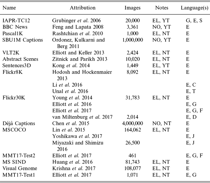
Table 1 provides an overview of image description datasets in terms of number of images, language(s) the descriptions are in, whether there is an explicit or implied real-world application task (e.g. news article image captioning), and whether they were elicited from contributors, or collected from sources where they occur naturally.
Image description datasets

EL = elicited; NO = naturally occurring; YT = there is a clear application task; NT = no task; G = German; E = English; S = Spanish; C = Mandarin; T = Turkish; F = French; D = Dutch; J = Japanese.
The IAPR-TC12 benchmark (Grubinger et al. Reference Grubinger, Clough, Müller and Deselaers2006a) has 20,000 images from a travel company’s photo collection each with text captions in German, English, and Spanish. The dataset was intended for benchmarking retrieval systems in ImageCLEF 2006. Images depict a wide range of travel-related topics, including sport, landmarks, animals, group shots, landscapes, etc. In contrast to other datasets reviewed here, the collection contains sets of images that depict very similar content (e.g. the same cathedral), but from different angles, dates, etc. Original annotations by the travel company were quality-checked, corrected, and completed by direct contributors (not crowdsourced). E.g. a photo of a brown sandy beach; the dark blue sea with small breaking waves behind it; a dark green palm tree in the foreground on the left; a blue sky with clouds on the horizon in the background.
The BBC News Database (Feng and Lapata Reference Feng and Lapata2008) contains 3,361 image-caption-document tuples collected from the BBC News website. Captions are often nondescriptive, e.g. Breastfed babies tend to be brighter for an image showing a baby being breastfed. The implicit image description task is news image caption generation, but Feng and Lapata use the data for image labeling.
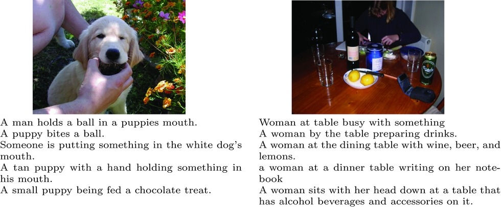
For Pascal1K, Rashtchian et al. (Reference Rashtchian, Young, Hodosh and Hockenmaier2010) used Mechanical Turk to collect five descriptions each for 1,000 VOC’08 images (50 selected randomly from each of the 20 VOC’08 classes). Contributors had to have high HIT rates and pass a language competence test, leading to relatively high text quality with few grammatical or spelling mistakes. Two example images and their descriptions are shown in Figure 1.
Two images from Pascal1K; original spelling errors (Rashtchian et al. Reference Rashtchian, Young, Hodosh and Hockenmaier2010).

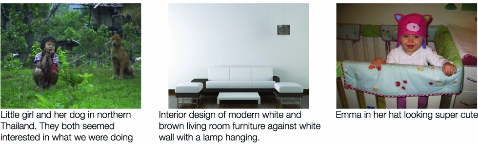
The SBU1M team collected one million Flickr images with naturally occurring captions (Ordonez et al. Reference Ordonez, Kulkarni and Berg2011), filtering initial search results to retain only images with captions containing at least two words from the original query, and at least one preposition (indicating visible spatial relationships). For examples see Figure 2.
Image and caption examples from SBU1M.

For VLT2K, Elliott and Keller (Reference Elliott and Keller2013) used the images from the VOC’11 action recognition taster competition (Everingham et al., 2011), and collected three descriptions per image via Mechanical Turk. Subsequent annotation steps added visual dependency relations, and associated image regions with descriptions.
The Abstract Scenes dataset (Zitnick and Parikh Reference Zitnick and Parikh2013) consists of 1,002 sets of ten similar abstract scenes and one associated description. Mechanical Turk contributors created individual scenes of children playing using clip art. Other contributors described the scenes using 1–2 sentences. Finally, contributors created nine more scenes to match each description. This dataset differs from the others in its use of cartoon-like scenes in which physical properties can be unrealistic.
The Sentences3D team (Kong et al. Reference Kong, Lin, Bansal, Urtasun and Fidler2014) collected descriptions and annotations for the 1,449 photos of indoor scenes in the NYU-RGBD v2 dataset via Mechanical Turk. Descriptions vary from one to ten sentences, and tend to be complex with multiple mentions of visual objects. Additional annotations (by direct contributors) link nouns and pronouns to the visual objects they describe.
Flickr8K has 8,092 images of people/animals performing some action from six Flickr groups (Hodosh, Young and Hockenmaier Reference Hodosh, Young and Hockenmaier2013). Five descriptions per image were collected via Mechanical Turk; QA measures were e.g. a spelling/grammar test, and location in the United States. Contributors were asked to write single sentences describing the depicted scenes, situations, events and entities. This dataset was extended in Flickr30K (Young et al. Reference Young, Lai, Hodosh and Hockenmaier2014) to 31,783 images. As a further extension, Multi30K (Elliott et al. Reference Elliott, Frank, Sima’an and Specia2016) added 31,014 German translations of the original English descriptions (one per image), and 155,070 German original image descriptions (five per image).
Extensions of Flickr30K to other languages exist. Van Miltenburg et al. annotated 2,014 images from the validation and test parts of Flickr30K with five Dutch descriptions each via Crowdflower, using the same collection regime (van Miltenburg, Elliott and Vossen Reference van Miltenburg, Elliott and Vossen2017). Unal et al. collected Turkish descriptions for Flickr8K, again using the same regime (Unal et al. Reference Unal, Citamak, Yagcioglu, Erdem, Erdem, Cinbis and Cakici2016). Li et al. extended the dataset to Chinese, creating Mandarin captions by (i) machine translating the original descriptions with Google and Baidu, and (ii) crowdsourcing new descriptions (Li et al. Reference Li, Lan, Dong and Liu2016).
Lin et al. collected two sets of image descriptions for the MS COCO corpus of 2.5 million labeled objects in 328,000 images, one containing five descriptions for every image in the training, validation and test sets; the other having forty descriptions each for a random subset of 5,000 test set images (Lin et al. Reference Lin, Maire, Belongie, Hays, Perona, Ramanan, Dollár and Zitnick2014a). The latter were collected with the aim of achieving higher correlation with human judgments in automatic evaluation via a large number of reference descriptions.
MMT-Test2 (which the MMT team call the Ambiguous COCO test data) is a collection of 461 MS COCO images selected for containing an ambiguous verb (fifty-six verbs in total), in a complex process (Elliott et al. Reference Elliott, Frank, Barrault, Bougares and Specia2017) that involved information from the VerSe dataset of ambiguous-verb captions (Gella, Lapata and Keller Reference Gella, Lapata and Keller2016).
The STAIR Captions dataset (Yoshikawa, Shigeto and Takeuchi Reference Yoshikawa, Shigeto and Takeuchi2017) is an extension of MS COCO to Japanese, with five descriptions for each MS COCO image, obtained with slightly different instructions, using crowdsourcing and direct contributions. An earlier Japanese MS COCO extension for a subset of 26,500 images crowdsourced 3–5 Japanese descriptions per image, again using a slightly different collection regime, including a caption quality filtering step at the end (Miyazaki and Shimizu Reference Miyazaki and Shimizu2016).
The Déjà Captions team collected 760 million image/text pairs from Flickr, using 693 frequent nouns for queries (Chen et al. Reference Chen, Kuznetsova, Warren and Choi2015a). They segmented texts into sentences and filtered out those that did not contain the query term. Only captions which very closely resembled at least one other caption for a different image were then retained. The result was a collection of 180 K unique captions for 4 million images. As with the Abstract Scenes dataset, there are multiple images per caption, whereas with other datasets in this section it is the other way round.
MS SIND (Huang et al. Reference Huang2016) is a dataset of story-like image sequences paired with: (1) descriptions for each image in isolation, (2) descriptions for each image when seen in a sequence, and (3) descriptions that form a narrative over an image sequence (images/sentences aligned). Image sequences were obtained from Flickr albums, only retaining ‘storyable’ albums with 10–50 photos, taken within 48 h.
The Visual Genome dataset (Krishna et al. Reference Krishna2017a) has region descriptions (in addition to six other annotation components) for 108,077 images, e.g. for an image with three regions: man jumping over a fire hydrant, yellow fire hydrant, and woman in shorts is standing behind the man.
MMT-Test1 (a.k.a. Multi30K 2017 test data) is a new dataset of images/texts collected from some of the same Flickr groups as Flickr30K, and some new groups (Elliott et al. Reference Elliott, Frank, Barrault, Bougares and Specia2017) in a multistep process, resulting in a final set of 1,071 images/texts, each supplemented by one professional German translation, and five crowdsourced German descriptions.
The datasets reviewed in this section differ on many dimensions, including size, ranging from a few thousand images (Pascal1K, BBC News, VLT2K) to a million and more (SBU1M, Déjà Captions). English remains the most frequent language, but other languages are being seen more frequently, mostly as extensions of English datasets. The images in all but one dataset (Abstract Scenes) are photos, mostly user-generated (except BBC News). In some cases, labeled object bounding boxes or region masks (VLT2K, MS COCO, Sentences3D, Visual Genome) around objects are available. Most datasets have image texts elicited from contributors for the specific purpose of creating the corpus, but some, including the very large datasets, have naturally occurring image texts (BBC News, SBU1M, Déjà Captions).
2.1.2 Collecting human-generated image descriptions
Quality assurance measures, instructions, and guidelines to contributors when eliciting image descriptions can vary substantively between datasets. The IAPR TC-12 descriptions were intended to describe ‘what can be recognized in an image without any prior information or extra knowledge’ (p. 6). The creators decided not to ask for full sentences, or for descriptions of the entire image, specifically to thwart people’s natural storytelling tendencies. They did not constrain the number of phrases that could be used or their order, and considerable variation can be seen in both. A typical example is a brown cathedral with two towers and three green doors; a square with street lamps, green spaces, flowers, a tree, benches, and people in front of it; grey cobblestones in the foreground; a hill and clouds in the background.
For VLT2K, Elliot and Keller placed similar restrictions on contributors, asking them to describe an image in two sentences, the first describing the action in the image, the person performing the action and the region involved in the action; the second describing any other regions in the image not directly involved in the action; e.g. A man is riding a bike down the road. A car and trees are in the background.
For most datasets, however, the only structural restriction is that descriptions should have one or two sentences describing the whole image. This allows a wide variety of style and focus which researchers seek to control by lists of DOs and DON’Ts which can be detailed. For example, for MS COCO:
• Please describe the image
• Describe all the important parts of the scene.
• Do not start the sentences with ‘There is’.
• Do not describe unimportant details.
• Do not describe things that might have happened in the future or past.
• Do not describe what a person might say.
• Do not give people proper names.
• The sentences should contain at least eight words.
Looking at image descriptions in datasets reveals that contributors do not always follow such instructions, producing descriptions such as: An empty boat begs to be used; The happy lady enjoys her surroundings; Take a solitude horse ride in the beautiful country; and The curious dog looks to do some damage to the pots. It appears that more rigorous control, as e.g. for IAPR-TC12 and VLT2K, is needed to constrain people to producing descriptions that describe only what can be seen.
2.1.3 How humans describe images
Human-authored image descriptions tend to prioritize mention of foregrounded and/or large entities, their attributes (color, size, etc.), and relationships linking them, to each other and to their surroundings. However, human authors have strong tendencies to add many different kinds of conjectured content, attributing emotions and intent to people and animals, placing the image in the context of a story, or ascribing subjective properties to image elements. The examples in Figure 1 exhibit several forms of conjecture. For the picture on the left, it is unclear whether the object in the dog’s mouth is a chocolate treat, a ball, or something else. Is the object being put into, held in, or in fact retrieved from, the dog’s mouth? Is it a puppy or a grown dog? Is its color white or tan? For the picture on the right, is the woman working on her notebook, preparing drinks, or is she busy with something unidentifiable? In the (naturally occurring) captions of the images in Figure 2 proper names, subjective attributes, and attribution of state of mind are all used.
From guessing emotional states to being more precise than the information in an image permits, people have a tendency to fill in the missing bits, to tell a story. Moreover, they do this in a myriad of different ways. On the one hand, humans have these tendencies, on the other hand researchers try to quell them and elicit descriptions that only talk about what can be seen in an image, moreover only what is ‘important.’ This strong pull between what people come up with when asked to describe an image, and what researchers try to get them to do, raises questions about whether this is a good way to collect training and evaluation data.
2.1.4 Human-generated image descriptions as training and evaluation data
The datasets above are used to train the methods in Section 2.2, and as reference data by many of the evaluation methods in Section 2.3. Systems are trained to produce similar image descriptions to those in these datasets, and the image descriptions they generate are considered good if they are similar to those in the datasets, yet there is a lack of clarity in the field regarding both (i) what these image texts are, and (ii) what they are meant to be for. Regarding the former, the main distinction drawn is between descriptions and captions. For example, Bernardi et al. (Reference Bernardi, Cakici, Elliott, Erdem, Erdem, Ikizler-Cinbis, Keller, Muscat and Plank2016) distinguish descriptions which ‘verbalize visual and conceptual information depicted in the image, i.e., descriptions that refer to the depicted entities, their attributes and relations, and the actions they are involved in’ (p. 4), and captions which ‘typically [. . .] verbalize information that cannot be seen in the image [providing] personal, cultural, or historical context for the image’ (p. 18). Similarly, Frank et al. in this volume ‘define descriptions as sentences that are solely and literally about an image, whereas captions are more naturalistic sentences associated with, but not necessarily descriptions of, an image’ (p. 3).
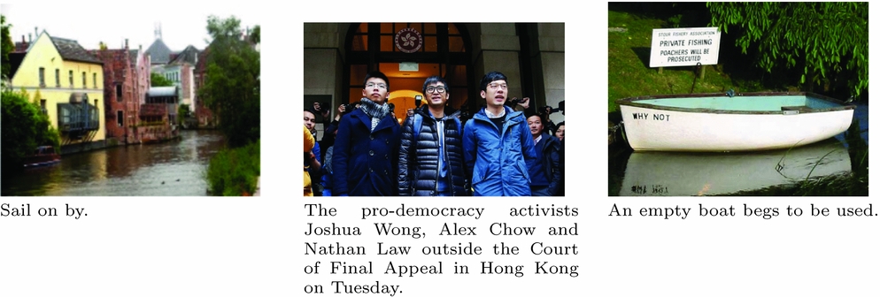
A text accompanying an image in a real-world context (e.g. a caption, article, title, alt text) can normally be unambiguously assigned to a category. Take away the context however, and it is far less clear what category a text belongs to. In Figure 3, for example the Flickr caption on the left makes no reference to anything visible in the image; the text in the middle is a caption from a news website, and is highly descriptive; the text on the right was elicited for Pascal1K as a description, but is very ‘caption-like’. All examples in Figure 2 are naturally occurring captions, but the first sentence on the left, and the whole caption in the middle, neatly fit both of the definitions of descriptions above.
From left: Image and caption from Déjà Captions; news image from New York Times, Feb 6 2018, 11:55 (https://www.nytimes.com/2018/02/06/world/asia/ hong-kong-joshua-wong-appeal.html); image and elicited description from Pascal1K.

The question is, does it make sense to say that a text that naturally occurs as a caption is not a caption because it does not fit some definition of captions? It seems more practical to say that a text is a caption because it appears in a particular place alongside an image, regardless of its textual properties, i.e. to tie the definition to application context. Systems trained on naturally occurring captions have this real-world grounding by default, and an implied application task: to generate the kinds of texts normally seen as captions in the particular context data was collected from.
Image description generation systems do not have this real-world grounding: there is no standard definition of what a description is, and there are no naturally occurring image texts unambiguously identifiable as descriptions. This has two implications: (i) for data collection: there is no obvious way to constrain the kinds of texts that should be elicited from contributors; and (ii) for evaluation: because elicited descriptions are used for both training and evaluation where systems are deemed good in proportion to the similarity of their output to the elicited descriptions, the result is a closed system in which questions of what collected tests are meant to be good for, and whether they are in fact good for it, are not directly addressed at all (Belz Reference Belz2009). This is why real-world grounding is needed: an explicitly stated application context would address both of these questions, an issue which we will pick up again in the section on extrinsic evaluation below (Section 2.3.3).
2.2 Image description methods
A basic division in image description is between (i) methods that create descriptions for new images from scratch, and (ii) methods that retrieve similar image/description pairs from the training data, and use those to create a description for a new image. The latter are a form of memory-based learning, known as retrieval-based methods in image description. These subdivide into methods that assess the similarity of new cases with known cases in visual space, and generate descriptions in textual space (Hodosh et al. Reference Hodosh, Young and Hockenmaier2013; Karpathy, Joulin and Fei-Fei Reference Karpathy, Joulin and Fei-Fei2014; Chen and Zitnick Reference Chen and Zitnick2015; Vinyals et al. Reference Vinyals, Toshev, Bengio and Erhan2015); and those, now the more common, which involve some form of joint modeling of the visual and textual spaces (Ordonez et al. Reference Ordonez, Kulkarni and Berg2011; Gupta, Verma and Jawahar Reference Gupta, Verma and Jawahar2012; Mason and Charniak Reference Mason and Charniak2014; Yagcioglu et al. Reference Yagcioglu, Erdem, Erdem and Cakici2015).
Methods that create a new description for a given image from scratch, often called generative methods (Lin et al. Reference Lin, Maire, Belongie, Hays, Perona, Ramanan, Dollár and Zitnick2014a; Elliott and de Vries Reference Elliott and de Vries2015; Fang et al. Reference Fang, Gupta, Iandola, Srivastava, Deng, Dollazr, Gao, He, Mitchell, Platt, Zitnick and Zweig2015; Ortiz, Wolff and Lapata Reference Ortiz, Wolff and Lapata2015), tend to have the following component steps: (1) Image analysis, sometimes broken down into (a) identification of type and, optionally, location of, objects and background/scene in the image, and (b) detection of attributes, relations and activities involving objects from Step 1; and (2) generation of a word string from a representation of the output from Step 1. Sometimes, a third, re-ranking step is added. The distinguishing difference between the two types of approaches is that retrieval-based approaches must consult a memory bank of training instances during application, whereas generative approaches create models that abstract away from the individual instances seen during training, generalize over them, and are usually in some respect more effective and/or efficient than consulting training instances individually during application.
The above division is into two contrasting paradigms, broad-strokes outlines of general approach, which do not imply specific techniques to implement them. In the next section, we select a small number of reference papers, provide a detailed description of the methods presented in them, and describe a set of paradigmatically similar methods in relation to them. In Section 2.2.3, we briefly highlight some current trends in the field. Given that a very recent survey reviews a large cross-section of image description methods in detail (Bernardi et al. Reference Bernardi, Cakici, Elliott, Erdem, Erdem, Ikizler-Cinbis, Keller, Muscat and Plank2016), we do not aim to provide an exhaustive survey of image description papers here.
2.2.1 Generative approaches
As laid out in more detail above, generative methods start with some form of image analysis, mapping images to representations that encode information intended to be more useful or efficient for generating descriptions than the raw pixel-grid values. These may be readily interpretable by humans (symbolic representations of objects, attributes, relations, ‘stuff’, etc.), or not (vectors of real numbers). For Step 1a, some systems identify labeled regions (Farhadi et al. Reference Farhadi, Hejrati, Sadeghi, Young, Rashtchian, Hockenmaier and Forsyth2010; Kulkarni et al. Reference Kulkarni, Premraj, Dhar, Li, Choi, Berg and Berg2011; Yatskar, Vanderwende and Zettlemoyer Reference Yatskar, Vanderwende and Zettlemoyer2014), others directly map images to words (Fang et al. Reference Fang, Gupta, Iandola, Srivastava, Deng, Dollazr, Gao, He, Mitchell, Platt, Zitnick and Zweig2015). Step 1b determines object attributes (Kulkarni et al. Reference Kulkarni, Premraj, Dhar, Li, Choi, Berg and Berg2011; Yatskar et al. Reference Yatskar, Vanderwende and Zettlemoyer2014), spatial relationships (Yang et al. Reference Yang, Teo, Daumé III and Aloimonos2011; Elliott and Keller Reference Elliott and Keller2013; Muscat and Belz Reference Muscat and Belz2017), activities (Elliott and Keller Reference Elliott and Keller2013; Yatskar et al. Reference Yatskar, Vanderwende and Zettlemoyer2014), etc. In Step 2, systems differ in linguistic knowledge brought to bear on the generation process. Some view the task as linearizing labels, relations, and attributes from Step 1 (Li et al. Reference Li, Kulkarni, Berg, Berg and Choi2011; Fang et al. Reference Fang, Gupta, Iandola, Srivastava, Deng, Dollazr, Gao, He, Mitchell, Platt, Zitnick and Zweig2015); others slot them into templates (Kulkarni et al. Reference Kulkarni, Premraj, Dhar, Li, Choi, Berg and Berg2011; Yang et al. Reference Yang, Teo, Daumé III and Aloimonos2011; Elliott and Keller Reference Elliott and Keller2013), yet others use grammar to construct descriptions (Mitchell et al. Reference Mitchell, Han, Dodge, Mensch, Goyal, Berg, Yamaguchi, Berg, Stratos and III2012; Kuznetsova et al. Reference Kuznetsova, Ordonez, Berg and Choi2014). Some approaches (Fang et al. Reference Fang, Gupta, Iandola, Srivastava, Deng, Dollazr, Gao, He, Mitchell, Platt, Zitnick and Zweig2015; Wang, Schwing and Lazebnik Reference Wang, Schwing, Lazebnik, Guyon, Luxburg, Bengio, Wallach, Fergus, Vishwanathan and Garnett2017) add a final re-ranking step, e.g. the latter uses CIDEr (see Section 2.3.2) to calculate a ‘consensus evaluation score’ between candidate captions and their nearest neighbors retrieved via a cross-modal embedding space.
The standard architecture that has emerged for generative image description comprises an encoder, usually a CNN (convolutional neural network), which maps images to more efficient and/or more task-suitable representations of themselves, and a decoder, an RNN (recurrent neural network) or LSTM (an RNN with long short-term memory), which maps the new representations to descriptions. In a typical example of this approach, Lu et al. (Reference Lu, Xiong, Parikh and Socher2017) use the last convolutional layer of a ResNet with dimensionality 2, 048 × 7 × 7 to produce encodings, obtaining a global image feature vector as the normalized sum over the spatial CNN feature vectors at each of the k grid locations. The decoder is a single layer LSTM with hidden vector size 512, which takes as input the global image feature vector from the CNN stage concatenated with the current word embedding vector, and produces a prediction of the next word as output. During training CIDEr is used to assess progress.
An increasingly common addition to this basic architecture is a visual attention mechanism, which typically produces a spatial map that identifies the specific image region(s) most relevant to the current word prediction task (Karpathy and Fei-Fei Reference Karpathy and Fei-Fei2015; Xu et al. Reference Xu, Ba, Kiros, Cho, Courville, Salakhudinov, Zemel and Bengio2015). Lu et al.’s (Reference Lu, Xiong, Parikh and Socher2017) contribution is a version that only switches on when needed, based on the insight that nonvisual words such as determiners, as well as other words in contexts where the predictive power of the preceding word(s) is particularly strong, do not benefit from visual attention. The key idea is that the model learns to extract a ‘visual sentinel’ vector from the decoder’s memory of visual and linguistic information; an adaptive context vector is modeled as a mixture of the spatially attended image features and the visual sentinel vector, the latter controlled by a weight called the ‘sentinel gate’. The diagrams below show the standard attention architecture (left) in comparison with Lu et al.’s adaptive extension (right), where V = [v 1, . . ., v L] are the spatial image features at time t, a t, 1, . . .a t, L the attention weights, h t the hidden state, s t the visual sentinel vector, βt the sentinel gate, c t the context vector, and  $\hat{c}_t$ the new adaptive context vector:

Karpathy and Fei-Fei (Reference Karpathy and Fei-Fei2015), in the image analysis step, detect objects with a Region CNN, pretrained on ImageNet and finetuned on the 200 ImageNet classes. They use the top 19 detected locations as well as the whole image, and compute representations (sets of vectors) based on the 19 bounding boxes (region-based embedding). They obtain a word-based embedding in the same space with a bi-RNN, and compute pairwise similarities between individual region and word vectors as their inner products. They then obtain an alignment that pairs multiple words to single regions with a Markov Random Field. The resulting single-region/multiword alignments are used in Step 2, which outputs a list of snippets for identified regions.
Gan et al. (Reference Gan, Gan, He, Pu, Tran, Gao, Carin and Deng2017b) also use a standard CNN-LSTM set-up, but extend each weight matrix of the conventional LSTM to an ensemble of tag-specific weight matrices (blue triangles below). The degree to which each member of the ensemble is used to generate a caption is tied to the image-dependent probability of the corresponding tag. The following diagram presents the generation process in outline:

2.2.2 Retrieval-based approaches
Gupta et al.’s (Reference Gupta, Verma and Jawahar2012) description generator is an archetypal example of a retrieval-based approach, and comprises the following five steps:
(1) Extract image features: RGB and HSV histograms for color; Gabor and Haar descriptors for texture; GIST for scene; SIFT for shape. Feature extraction is repeated (except GIST) for three vertical and three horizontal image slices. Finally, vectors are concatenated into a single feature vector for each feature type.
(2) Retrieve k nearest images: compute distance between image feature vectors, using L 1 distance for color vectors, L 2 for texture and scene, χ2 for shape. Image distance is then the dot product of distance weights and feature vectors.
(3) Parse the descriptions of the k most similar images, using the Stanford dependency parser; extract object 1-tuples (subjects and objects), attribute/object 2-tuples (attribute + subject, attribute + object), action 2-tuples (e.g. verb + subject), and relation 3-tuples (e.g. verb + preposition + object) from the dependency parse.
(4) Compute a probability score for each candidate tuple (any tuple derived from one of the k retrieved descriptions) on the basis of relative image similarity (compared to the other k − 1 most similar images) and relative Google frequency (compared to the other candidate tuples). Tuples are ‘integrated’ by slotting them into a predefined tripartite syntactic template.
(5) Score the resulting ‘triples’ with the joint probability of their component tuples. Depending on the dataset, the top-scoring triple or the syntactically aggregated top three triples are passed to SimpleNLG for surface realization.
One of two seminal papers in the retrieval-based area, Ordonez et al. (Reference Ordonez, Kulkarni and Berg2011) present a simpler method that uses GIST and tiny-image for Step 1, and the sum of GIST similarity and tiny-image color similarity for Step 2. Following re-ranking of the most similar images, Steps 3–5 are trivial as the description of the top image is simply transferred as the output description. Kulkarni et al. (Reference Kulkarni, Premraj, Dhar, Li, Choi, Berg and Berg2011) and Yang et al. (Reference Yang, Teo, Daumé III and Aloimonos2011) use approaches similar to Gupta et al. for Step 3, but apply different syntactic templates in Step 4. Some techniques are familiar from generative approaches, e.g. Yagcioglu et al. (Reference Yagcioglu, Erdem, Erdem and Cakici2015) use encodings produced by a CNN trained on ImageNet for Step 1. Mason and Charniak (Reference Mason and Charniak2014) construe Step 4 as multidocument extractive summarization over the retrieved descriptions.
The above methods do not involve representations in a shared visual-textual space. Other retrieval-based methods, in addition to image similarity, also assess the match between possible descriptions and the input image. For example, Farhadi et al. (Reference Farhadi, Hejrati, Sadeghi, Young, Rashtchian, Hockenmaier and Forsyth2010), in the original retrieval-based method, map both images and descriptions to <object, action, scene > triples, using small multilabel Markov random fields. They consider the top k triples predicted for images and descriptions, and compute a rank-based similarity measure to select the description to be transferred.
Hodosh et al. (Reference Hodosh, Young and Hockenmaier2013) construe image description explicitly as a matter of ranking candidate descriptions, and the natural inverse of image retrieval, best implemented by a uniform approach. They focus on the problem of learning an appropriate mapping between images and descriptions for which they use Kernel Canonical Correlation Analysis with a wide range of different image and text kernels. Learned projection weights map KCCA image and description vectors to an induced shared space in which images are expected to appear nearer sentences they are more strongly associated with (i.e. that describe them well). Candidate descriptions are ranked in order of their cosine similarity in this space with the new image to be described.
2.2.3 Some recent trends
Attention mechanisms have been garnering increasing interest as additions to encoder–decoder architectures for image description (Xu et al. Reference Xu, Ba, Kiros, Cho, Courville, Salakhudinov, Zemel and Bengio2015; You et al. Reference You, Jin, Wang, Fang and Luo2016; Lu et al. Reference Lu, Xiong, Parikh and Socher2017), with extensions to the basic mechanism emerging. For example, You et al. selectively attend to candidate semantic concepts, fusing them into hidden states and outputs. Lu et al. (see above) introduce a selective visual attention mechanism that switches off when not needed.
Another trend is region-based image description (Karpathy and Fei-Fei Reference Karpathy and Fei-Fei2015; Krishna et al. Reference Krishna, Zhu, Groth, Johnson, Hata, Kravitz, Chen, Kalantidis, Li, Shamma, Bernstein and Fei-Fei2017b; Kinghorn, Zhang and Shao Reference Kinghorn, Zhang and Shao2018). E.g. the latter use a regional object detector and RNN-based attribute prediction in addition to encoder–decoder language generation, e.g. performing well at cross-domain generalization.
There is a growing interest in incorporating high-level concepts into neural architectures, rather than relying on lower-level image features alone. One approach trains a CNN classifier for each attribute (word) in the training descriptions (Wu et al. Reference Wu, Shen, Wang, Dick and van den Hengel2017); the resulting set of attribute likelihoods for an image is viewed as a high-level representation of its content. An RNN then generates captions on the basis of the attribute likelihoods. Similarly, Gan et al. (Reference Gan, Gan, He, Pu, Tran, Gao, Carin and Deng2017) compute tags (words) from images, and use the probability of each tag to compose the parameters in an LSTM (see Section 2.2.1).
More generally, bringing linguistic knowledge into neural-based image description is being explored. One approach uses dependency trees to embed sentences for image retrieval (Socher et al. Reference Socher, Karpathy, Le, Manning and Ng2014); another (Venugopalan et al. Reference Venugopalan, Hendricks, Mooney and Saenko2016) integrates a neural LM and distributional semantics obtained from large text corpora into an LSTM for video description. The ACL 2018 Workshop on Relevance of Linguistic Structure in Neural Architectures for NLP is a sign of growing interest.
Other recent developments are generating captions with creativity (Chen et al. Reference Chen, Kuznetsova, Warren and Choi2015a), sentiment (Mathews, Xie and He Reference Mathews, Xie and He2016), and humorous/romantic/plain styles (Gan et al. Reference Gan, Gan, He, Gao and Deng2017a); unsupervised learning of image-to-text mappings (Hendricks et al. Reference Hendricks2016); and generating paragraph-long descriptions (Krause et al. Reference Krause, Johnson, Krishna and Fei-Fei2017).
2.3 Evaluation of image description methods
A range of evaluation methods have been used in image description. Using the taxonomy developed in previous work (Belz and Hastie Reference Belz and Hastie2014), we distinguish the following method categories. Intrinsic measures assess properties of systems or components in their own right, for example comparing their outputs to model outputs in a corpus, whereas extrinsic measures assess the effect of a system on something that is external to it, for example human performance at a given task or the value added to an application. One subcategory of intrinsic methods are output quality measures, which can be either automatically assessed or human-assessed. Subcategories of extrinsic measures are user task success measures, which assess impact on users’ ability to perform a given task, and system purpose success measures, which assess impact on a system’s achievement of (an aspect of) its stated purpose.
By far the most common evaluation measures in image description are intrinsic assessments of output quality. Both automatic and human-assessed measures have been used, and we assess each of those in turn below (Sections 2.3.2 and 2.3.1). In Section 2.3.3, we briefly review the few extrinsic measures in the field.
2.3.1 Intrinsic human-assessed output-quality measures
Human assessment of the quality of generated outputs in image description tends to take the form of asking participants, mainly on crowdsourcing platforms, to answer questions about aspects of the texts, by selecting a score on a verbal descriptor scale of 1–3 or 1–5 where each number is accompanied by an explanatory bit of text. For example, Elliot and Keller crowdsourced five judgments each for 101 image/description pairs, using three criteria assessed on scales of 1–5:
(1) Grammaticality: give high scores if the description is correct English and doesn’t contain any grammatical mistakes.
(2) Action: give high scores if the description correctly describes what people are doing in the image.
(3) Scene: give high scores if the description correctly describes the rest of the image (background, other objects, etc).
Gupta et al. (Reference Gupta, Verma and Jawahar2012) collected human judgements on 100 and 500 images from the Pascal and IAPR TC-12 datasets, respectively, using rating criteria of Readability and Relevance, and scales from 1–3, adopted from Li et al. (Reference Li, Kulkarni, Berg, Berg and Choi2011).
The Readability and Grammaticality criteria above seek to assess if a text is the kind of text a native speaker would produce (most commonly called ‘Grammaticality’); the other criteria address aspects of what is called Adequacy in MT, in this context the appropriateness of the text for the image. Grammaticality (e.g. Kulkarni et al. Reference Kulkarni, Premraj, Dhar, Li, Choi, Berg and Berg2011; Li et al. Reference Li, Kulkarni, Berg, Berg and Choi2011; Yang et al. Reference Yang, Teo, Daumé III and Aloimonos2011; Gupta et al. Reference Gupta, Verma and Jawahar2012; Kuznetsova et al. 2012; Mitchell et al. Reference Mitchell, Han, Dodge, Mensch, Goyal, Berg, Yamaguchi, Berg, Stratos and III2012; Elliott and Keller Reference Elliott and Keller2013; Hodosh et al. Reference Hodosh, Young and Hockenmaier2013) and Adequacy (e.g. Li et al. Reference Li, Kulkarni, Berg, Berg and Choi2011; Yang et al. Reference Yang, Teo, Daumé III and Aloimonos2011; Gupta et al. Reference Gupta, Verma and Jawahar2012; Kuznetsova et al. Reference Gupta, Verma and Jawahar2012; Mitchell et al. Reference Mitchell, Han, Dodge, Mensch, Goyal, Berg, Yamaguchi, Berg, Stratos and III2012; Elliott and Keller Reference Elliott and Keller2013) are the two most common criteria used in the field. Other criteria have been used, for example Creativity (Li et al. Reference Li, Kulkarni, Berg, Berg and Choi2011), and Human-likeness (Mitchell et al. Reference Mitchell, Han, Dodge, Mensch, Goyal, Berg, Yamaguchi, Berg, Stratos and III2012).
The 2015 COCO Image Captioning Challenge took a different approach. Here, texts generated by all 15 competing systems, plus human and random texts, were assessed on five criteria; scores were derived either from verbal descriptor scale judgments, or the assessors’ response was converted to a percentage, as follows:
(1) Overall caption quality:
(a) Percentage of captions evaluated as better or equal to human caption.
(b) Percentage of captions that pass the Turing test.
(2) Correctness: Average correctness of the captions on a scale 1–5 (incorrect–correct).
(3) Detailedness: Average detail of the captions from 1–5 (lacking details–very detailed).
(4) Saliency: Percentage of captions that are similar to human description.
Two criteria are assessed on verbal descriptor scales as above, with Correctness a form of Adequacy. However, with the other criteria the organizers made an attempt to reduce subjectivity and variability in judgments by making them comparative.
Reporting of human-assessed evaluation experiments in noncompetition contexts in the field is frequently patchy, omitting crucial details such as how many evaluators were used, who they were, or reporting statistical significance assessments without giving the method used for the assessment. Human assessment is notoriously hard to reproduce and compare across experiments even where those involve the same data; an established standard framework of assessment criteria, experimental design, and contributor recruitment would go some way toward addressing this.
2.3.2 Intrinsic automatic output-quality measures
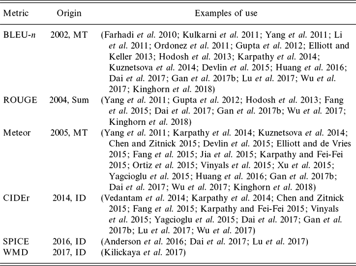
The main automatic metrics for assessing output quality that have been used in image description are BLEU and Meteor from machine translation, ROUGE from summarization, and CIDEr and SPICE that were specifically developed for evaluation of image descriptions. Table 2 presents an overview of metrics, the field they originated in, when they were introduced, and a sample of papers they have been used in. Below, we briefly summarize the metrics developed for image description (assuming the other three are well enough known).
Intrinsic output-quality metrics that have been used in image description

CIDEr (Vedantam, Zitnick and Parikh Reference Vedantam, Zitnick and Parikh2014) differs from other n-gram metrics such as BLEU mainly in that it assigns lower weights to n-grams that are common to reference image descriptions (using tf-idf).
SPICE (Anderson et al. Reference Anderson, Fernando, Johnson and Gould2016) starts by dependency-parsing the generated sentence and the reference sentences, then maps the result to a ‘scene graph’ of objects, relations, and object attributes. It constructs the union of scene graphs for the reference sentences, then turns both the graph for the generated sentence, and the union-graph for the reference sentences into tuple sets comprising 1-tuples for objects, 2-tuples for attributes, and 3-tuples for relations. Finally, Recall, Precision, and F-score are computed on the two tuple sets.
Most recently, Kilickaya et al. have proposed the use of the word mover distance (WMD) document similarity metric for image description (Kilickaya et al. Reference Kilickaya, Erdem, Ikizler-Cinbis and Erdem2017). WMD is similar in spirit to edit-distance metrics and computes the distance between generated text and reference text on the basis of the Euclidean distance between word2vec embeddings of words used as the cost of replacing one word with another.
Other metrics have been used, e.g. where a system produces ranked outputs, model performance can be measured by the rank of the original image or caption in the ranked list of outputs, e.g. R@k (Recall at k) is the percentage of queries for which the correct response was among the first k results; median rank of the correct response in the ranked list of results is also used (Hodosh et al. Reference Hodosh, Young and Hockenmaier2013).
Some research has shown Meteor to correlate well with human judgments in this field (Huang et al. Reference Huang2016). The paper that introduced CIDEr (Vedantam et al. Reference Vedantam, Zitnick and Parikh2014) found that the latter outperformed Meteor in most cases, but by a small margin. Evaluated on the 2015 COCO Challenge test data and human judgments for all five assessment criteria (see previous section for details), SPICE was shown (Anderson et al. Reference Anderson, Fernando, Johnson and Gould2016) to correlate far better with the human judgments than any of the other metrics discussed above in terms of Pearson’s r, with extremely high values for r except for detailedness, which it clearly is not suitable for. WMD has not been shown to clearly outperform SPICE (Kilickaya et al. Reference Kilickaya, Erdem, Ikizler-Cinbis and Erdem2017).
The aim of meta-evaluation is often presented as determining which metric is best at predicting human judgment, not which metric is best at assessing a specific criterion (best = strongest correlation with human assessments of the same criterion). Clearly, the metrics in this section are not suitable for assessing how detailed a description is (only if a description is as detailed as the average human one); SPICE is not suitable for Fluency, BLEU is, etc. Which metric is best depends on the assessment criterion. The evidence currently is that SPICE, CIDEr, and Meteor, in this order, predict human Adequacy and Grammaticality assessments well.
2.3.3 Extrinsic evaluation measures
An extrinsic form of evaluation for image description, more specifically a user-task-success measure, was proposed by Ordonez et al. (Reference Ordonez, Kulkarni and Berg2011) who presented contributors on Mechanical Turk with two images and one caption, and asked them to assign the caption to the ‘more relevant’ image. One of the two images was a system-generated one, whereas the other was selected randomly from the dataset. One of the ‘systems’ evaluated was the set of original human descriptions. The evaluation involved hundred images and showed that contributors were able to identify the correct picture from an original human description 96% of the time. For the best system, contributors were able to select the correct image 66.7% of the time.
Huang et al. (Reference Huang2016) used crowdsourcing to ask five contributors per story to rate how strongly they agreed with the statement If these were my photos, I would like using a story like this to share my experience with my friends (on a Likert-type scale of ‘strongly disagree’ to ‘strongly agree’). This measure can be seen as assessing system purpose success (see above), in terms of the likelihood that end users will actually use the image-series descriptions generated by systems. However, rather than evaluate actual use rates in a real-world context such as Flickr, contributors are asked to judge how likely they would be to use the texts in a real-world context. This is a surrogate measure reminiscent of the ‘pseudoextrinsic’ measure of Overall Responsiveness used in the TAC’08 summarization competition where the question was What would I pay for this summary of the answers to my questions?
In many situations, real-world extrinsic evaluation is not feasible, simply because it is expensive and time-consuming to set up and run. However, extrinsic grounding, where an application task is explicitly defined, data is collected within the context of the application task, and evaluations can be carried out by comparing against extrinsically grounded reference data, should be feasible in many situations, and would help begin to address the vexed questions from Section 2.1.4.
3 Referring expression generation and comprehension
Much of everyday language and discourse concerns the visual world around us; this makes understanding the relationship between objects in the physical world and language describing the objects an important challenge for AI. While image description strives to construct broad descriptions of image content, referring expressions, REs, are a more focused form of language, used to identify a particular object or temporal event in an image or video. People use such expressions all the time, especially in dialogue to indicate a particular object or event to a co-observer, e.g. the woman in the blue shirt, or when she took a bite of the apple. Computational models that generate and comprehend such expressions have broad applicability to human–computer interaction, especially for agents such as robots, interacting with people in the real world. Successful models need to connect visual interpretations of objects in the world to natural language that describes an object or event.
In the RE problem, there is a pragmatic interaction between agents that involves two main tasks: (a) a speaker task where one must generate a natural language expression given a target and its surrounding world context; and (b) a listener task where one must interpret and comprehend the expression and map it to the correct target. We refer to these two tasks as REG and comprehension, respectively. In this section, we review work on REs, including datasets and methods for generation and comprehension in images and videos.
3.1 Referring expression datasets
Some initial datasets in REG used graphics engines to produce images of objects (van Deemter, van der Sluis and Gatt Reference van Deemter, van der Sluis and Gatt2006; Viethen and Dale Reference Viethen and Dale2008) with corresponding shared evaluation challenges (Gatt and Belz Reference Gatt and Belz2010). Recently more realistic datasets have been introduced, consisting of craft objects like pipecleaners, and ribbons (Mitchell, van Deemter and Reiter Reference Mitchell, van Deemter and Reiter2010), or everyday home and office objects such as staplers or combs (Mitchell, Reiter and van Deemter Reference Mitchell, Reiter and van Deemter2013a), arrayed on a simple background. These datasets helped move REG research into the domain of real world objects.
In the past few years, datasets have become even larger and more realistic and expanded to include video REs. The ReferIt Dataset (Kazemzadeh et al. Reference Kazemzadeh, Ordonez, Matten and Berg2014) was perhaps the first large-scale RE dataset to be based on complex real world scenes. The images used to construct this dataset were originally sampled from the ImageCLEF IAPR image retrieval dataset (Grubinger et al. Reference Grubinger, Clough, Müller and Deselaers2006b), a large collection of scene images with associated object segmentations. The ReferIt dataset was collected via a simple two-player online game (the ReferItGame) to crowdsource REs. In this game, Player 1 is shown an image with a highlighted target object and asked to write a natural language expression referring to the target. Player 2 is shown only the image and RE and asked to click on the corresponding object. If the players do their job correctly, they receive points and the expression is added to the dataset. This allows both data collection and verification within the game.
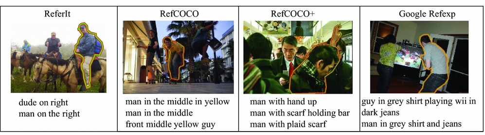
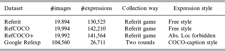
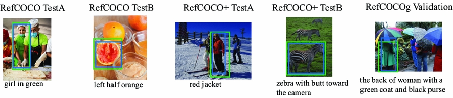
Based on this game, Yu et al. (Reference Yu, Ko, Choi and Kim2016a) further collected the RefCOCO and RefCOCO+ datasets, building on the MS COCO image collection (Lin et al. Reference Lin, Maire, Belongie, Hays, Perona, Ramanan, Dollár and Zitnick2014b). In the RefCOCO dataset, no restrictions are placed on the type of language used in the REs, while in the RefCOCO+ dataset players are stopped from using location words in their REs by adding ‘taboo’ words to the ReferItGame. Thus, RefCOCO+ tends to focus more on appearance based descriptions. Another dataset based on MS COCO images has been collected, called the Google Refexp dataset (Mao et al. Reference Mao, Huang, Toshev, Camburu, Yuille and Murphy2016). During collection of this dataset, one set of workers on Mechanical Turk were asked to write REs for objects. Another set of workers were asked to click on the indicated object given an RE. In Table 3, we show the statistics of each of the above-mentioned four datasets. REs in RefCOCO and RefCOCO+ tend to contain fewer words than those in Refexp since the competitive and time-based nature of games encourages players to write only the amount of information necessary to convey the correct object to the other player. Refexp contains more caption-like REs with many details about each referred object since labelers were encouraged to do so. Figure 5 shows example images and expressions.
Example images and referring expressions from RE datasets.

Example video and temporal RE in DiDeMo (Hendricks et al. Reference Hendricks, Wang, Shechtman, Sivic, Darrell and Russell2017).

Four referring expression datasets that use realistic images

More recently, inspired by the two-player game GuessWhat, a task for localizing an unknown object by comprehending a sequence of questions and answers was introduced (De Vries et al. Reference De Vries, Strub, Chandar, Pietquin, Larochelle and Courville2017). An example sequence is (‘Is it a vase?’, ‘Yes’), (‘Is it in the left corner?’, ‘No’), (‘Is it the purple one?’, ‘Yes’), etc.
In addition to image-based RE datasets, in the past year several video-based RE datasets and related tasks have been proposed. One example is the task of RE-guided tracking where a natural language specification indicates what object to track in a video (Li et al. Reference Li2017). Other work (Hendricks et al. Reference Hendricks, Wang, Shechtman, Sivic, Darrell and Russell2017) considers retrieving a specific temporal video segment (a moment rather than an object) given a natural language text description. They introduce a dataset called Distinct Describable Moments (DiDeMo) with language annotations of video segments. We show an example of a video-expression pair in Figure 4. The whole dataset consists of 40,000 pairs of localized video moments and corresponding expressions.
3.2 Referring expressions for images
Research on understanding how people generate REs has a long history, dating back to the 1970s (Winograd Reference Winograd1972). Early work in REG (Dale and Reiter Reference Dale and Reiter1995, Reference Dale and Reiter2000) explored research related to the Gricean maxims (Grice Reference Grice1975) which provide principles for how people will behave in conversation, including quality, , quantity, relevance, and manner. More recently, there has been progress examining other aspects of the RE problem such as types of attributes used (Mitchell et al. Reference Mitchell, Reiter and van Deemter2013a), modeling variations between speakers (Viethen and Dale Reference Viethen and Dale2010; Van Deemter et al. Reference Van Deemter, Gatt, van Gompel and Krahmer2012; Mitchell, van Deemter and Reiter Reference Mitchell, van Deemter and Reiter2013b; Viethen, Mitchell and Krahmer Reference Viethen, Mitchell and Krahmer2013), incorporating visual classifiers (Mitchell, van Deemter and Reiter Reference Mitchell, van Deemter and Reiter2011), producing algorithms to refer to object sets (Ren, Van Deemter and Pan Reference Ren, Van Deemter and Pan2010; FitzGerald, Artzi and Zettlemoyer Reference FitzGerald, Artzi and Zettlemoyer2013), or examining impoverished perception REG (Fang et al. Reference Fang, Liu, She and Chai2013). There have been REG shared-task competitions since 2007 (Gatt and Belz Reference Gatt and Belz2010). Krahmer and van Deemter provide a good survey of work in this area (Krahmer and van Deemter Reference Krahmer and van Deemter2012).
In the past few years, deep learning techniques have been widely applied in RE research. In the following, we denote r as the RE and o as the target object. As described above, there are typically two tasks explored in the literature. The first task is referring expression comprehension, requiring a system to select the region described by a given RE. To address this problem, some work (Hu et al. Reference Hu, Xu, Rohrbach, Feng, Saenko and Darrell2016; Mao et al. Reference Mao, Huang, Toshev, Camburu, Yuille and Murphy2016; Nagaraja, Morariu and Davis Reference Nagaraja, Morariu and Davis2016; Yu et al. Reference Yu, Poirson, Yang, Berg and Berg2016a) models P(r|o), selecting the object o from the image that maximizes this probability. Alternatively, some works model P(o, r) directly (Rohrbach et al. Reference Rohrbach, Rohrbach, Hu, Darrell and Schiele2016; Wang, Li and Lazebnik Reference Wang, Li and Lazebnik2016a; Liu et al. Reference Liu2017; Wang et al. Reference Wang, Li, Huang and Lazebnik2018; Yu et al. Reference Yu, Lin, Shen, Yang, Lu, Bansal and Berg2018), by learning an embedding that minimizes the distance between object-expression pairs. The second task is REG, which asks a system to compose a natural language expression for a specified object within an image, i.e. P(r|o). Many recent works (Mao et al. Reference Mao, Huang, Toshev, Camburu, Yuille and Murphy2016; Yu et al. Reference Yu, Poirson, Yang, Berg and Berg2016a; Liu et al. Reference Liu2017) use CNN-LSTM structures to generate expressions.
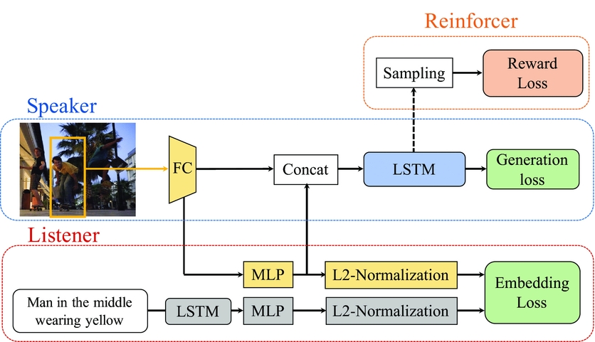
One current state-of-art model is the speaker–listener–reinforcer model (Yu et al. Reference Yu, Tan, Bansal and Berg2017), a unified framework for comprehension and generation tasks (see Figure 6). The speaker module generates REs, the listener comprehends REs, and the reinforcer uses a reward function to guide sampling of more discriminative expressions. The speaker is modeled using a CNN-LSTM framework. VGGNet (Simonyan and Zisserman Reference Simonyan and Zisserman2015) is used to extract a visual representation for the target object and other visual context. Then, an LSTM (Hochreiter and Schmidhuber Reference Hochreiter and Schmidhuber1997) is used to generate the most likely expression given the visual representation. Given a target object o i, its VGG-fc7 feature v i is first extracted. Its global context g i, is modeled as features extracted from the VGG-fc7 layer for the entire image. Finally, its location/size is modeled as a five-dimensional vector, l i, encoding the top-left and bottom-right corners of o i, as well as its relative size with respect to the image, i.e.  $l_i=[\frac{x_{tl}}{W}, \frac{y_{tl}}{H}, \frac{x_{br}}{W}, \frac{y_{br}}{H}, \frac{w\cdot h}{W\cdot H}]$. The speaker model also considers visual comparisons to produce expressions contrasting the target object from other related objects. The comparison features are composed of (a) appearance similarity δv i, and (b) location and size similarity δl i. The final visual representation for the target object is a concatenation of the above features followed by a fully connected layer fusing them together, r i = W m[v i, g i, l i, δv i, δl i] + b m. This joint feature is then fed into the LSTM for RE generation. During training the negative log-likelihood is minimized:
 \begin{align}
\begin{split} L_1^s(\theta ) & = -\sum _i \log P(r_i|o_i;\theta ) \\
& = -\sum _i \sum _t \log P(r^t_i|r^{t-1}_i, \ldots , r^1_i, o_i;\theta ) \end{split}
\end{align}
 $$\begin{equation}
\begin{split} L^l(\theta ) = \sum _i [ \lambda ^l_1 \max (0, M+S(r_i, o_k)-S(r_i, o_i)) \\
+\, \lambda ^l_2 \max (0, M+S(r_j, o_i) - S(r_i, o_i))] \end{split}
\end{equation}$$
Joint speaker–listener–reinforcer model for RE generation/comprehension (Yu et al. Reference Yu, Tan, Bansal and Berg2017).

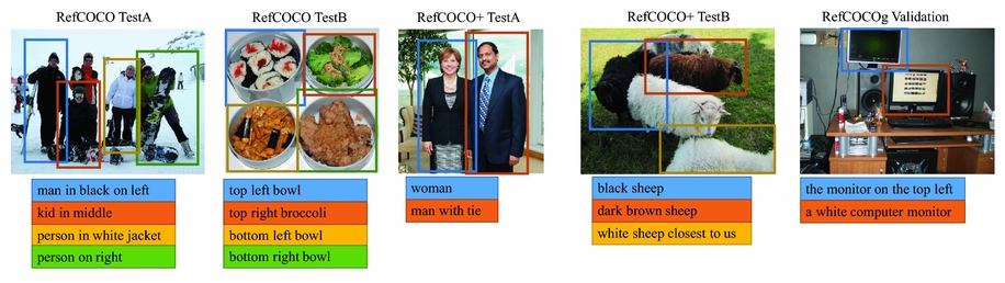
Comprehension examples in Yu et al. (Reference Yu, Tan, Bansal and Berg2017). Green box shows the ground-truth region, blue box shows correct comprehension using the proposed model.

Generation examples in Yu et al. (Reference Yu, Tan, Bansal and Berg2017). Each sentence shows the generated expression for one of the depicted objects (color coded to indicate correspondence).

3.3 Referring expressions for video
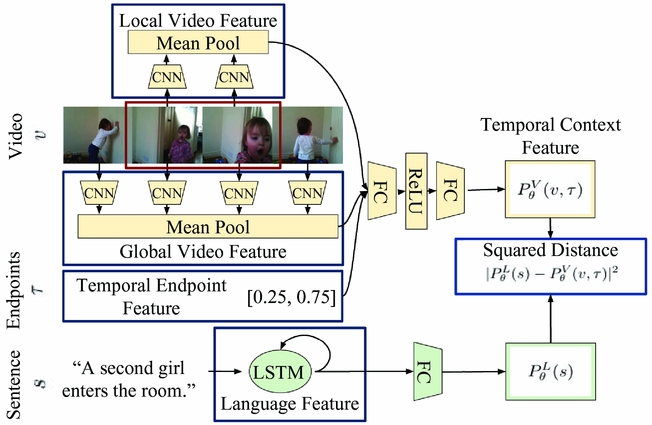
To address the temporal localization task (Figure 4) the Moment Context Network (MCN) was proposed (Hendricks et al. Reference Hendricks, Wang, Shechtman, Sivic, Darrell and Russell2017). Given input video frames v = v t where t ∈ 0, . . ., T − 1 indexes time, a proposed temporal interval  $\hat{\tau }=\tau _{\mbox{start}}:\tau _{\mbox{end}}$, and an expression r, the goal is to find the moment described by r:
 $$\begin{equation}
\hat{\tau } = \mbox{argmin}_{\tau } D_{\theta }(s, v, \tau )
\end{equation}$$
Moment Context Network (MCN) used in Hendricks et al. (Reference Hendricks, Wang, Shechtman, Sivic, Darrell and Russell2017).

To construct the local and global visual features, fc7 features are extracted for each frame using VGGNet. Then, the local features are constructed by temporally pooling features within each specific moment, and global features are constructed by averaging over all video frames. Temporal endpoint features indicate the start and endpoint of a candidate moment (normalized to the interval [0,1]). The concatenation of these features are fed into a MLP to get the final visual feature for a moment PV θ. Additionally, the authors also incorporate optical flow (Wang et al. Reference Wang, Xiong, Wang, Qiao, Lin, Tang and Van Gool2016b) as a motion feature for each moment PF θ. The language encoding is similar to Yu et al. (Reference Yu, Tan, Bansal and Berg2017), where an LSTM is used to encode the input expression and its last hidden state is fed into a MLP to yield the embedded feature PL θ. Then, the distance between a moment and an RE is computed as
 $$\begin{equation}
D_{\theta }(r, v, t) = \Vert P_{\theta }^V(v, \tau ) - P_{\theta }^L(r) \Vert + \eta \Vert P_{\theta }^F(f, \tau ) - P_{\theta }^L(r) \Vert
\end{equation}$$
4 Visual question answering
Another language and vision task that has received increasing attention recently is VQA. VQA systems take as input an image or video along with relevant natural language questions, and produce an answer to those questions. Questions can be open ended, requiring systems to produce a natural language answer, or a set of multiple choice answers is provided, requiring systems to select the best answer from a list. One driving factor for the introduction of VQA was that despite progress on image and video captioning, automatic evaluation of descriptions is still a challenging open research problem. Multiple choice VQA provides a task that is simple to evaluate automatically. Additionally, VQA provides a nice tool for more fine-grained evaluation of algorithms since different types of questions can be used to probe and evaluate various aspects of visual understanding, ranging from object identification, counting, or appearance, to more complex visual understanding of interactions, and inferences about why or how something is occurring in an image or video. In this section, we describe existing VQA datasets and review some efforts toward building VQA systems.
4.1 VQA in images
4.1.1 Image-based VQA datasets
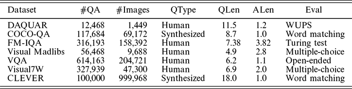
Several VQA datasets have recently been constructed. We review some of the prominent efforts here. Statistics about all of the datasets are presented in Table 4.
Image VQA Dataset statistics, including: number of question–answer pairs (#QA), number of images (#Images), question type (QType), average question length (QLen), average answer length (ALen), and evaluation type (Eval)

DAQUAR (Malinowski and Fritz Reference Malinowski and Fritz2014) was built on the NYU indoor scene RGB-D dataset (Silberman et al. Reference Silberman, Hoiem, Kohli and Fergus2012), a collection of indoor environments with associated RGB and depth camera images and annotated object class labels. To construct the dataset, the DAQUAR authors asked five in-house participants to provide questions and answers based on these images. Questions generally refer to everyday objects and relationships between objects, e.g. ‘Q: what is on the right side of the notebook on the desk in image4, A: plastic cup of coffee’. Answers are evaluated using the WUPS score to compute how close the produced answer from a system matches the ground truth answer. WUPS is a soft measure based on the Wu and Palmer score (Wu and Palmer Reference Wu and Palmer1994), which calculates the semantic relatedness of terms by considering the depths of their synsets in the WordNet taxonomy, along with the depth of the least common subsumer.
COCO-QA (Ren, Kiros and Zemel Reference Ren, Kiros and Zemel2015a) is built on the MS COCO dataset (Section 2.1.1). QA pairs are automatically generated from image descriptions using four question templates: Object Questions, Number Questions, Color Questions, and Location Questions. For example, a description reading ‘A man is riding a horse’ can be automatically transformed into the question ‘What is the man riding?’ Each answer consists of a single word, allowing models to treat the problem as a classification task without considering natural language generation, simplifying evaluation.
FM-IQA (Gao et al. Reference Gao, Mao, Zhou, Huang, Wang and Xu2015) is also built on MS COCO (FM stands for Freestyle Multilingual). Annotators provide freestyle question–answer pairs in Chinese, then each question–answer pair is translated into English. Arguing that automatic metrics like WUPS, BLEU, METEOR, or CIDEr cannot accurately evaluate model capacity, the authors conduct a Visual Turing Test (Turing Reference Turing1950) instead, where answers are mixed between humans and model, then human judges are asked to distinguish models from humans, and provide a score indicating the answer quality.
Visual Madlibs (Yu et al. Reference Yu, Park, Berg and Berg2015) is again built on MS COCO. Questions are designed with twelve fill-in-the-blank templates, to collect targeted descriptions about: people and objects, their appearance, activities, and interactions, as well as inferences about the general scene or its broader context. Collected descriptions are used for two tasks: (a) fill-in-the-blank description generation (similar to image captioning, but more focused on a particular image aspect), and (b) multiple-choice fill-in-the-blank question answering. In the latter, given an image and a partial description such as ‘The person is [blank] the frisbee’, the task is to select the correct choice from four answers. This provides an multiple-choice test for evaluation; varying the selection of negative answers can make questions for model testing easier or harder.
VQA (Antol et al. Reference Antol, Agrawal, Lu, Mitchell, Batra, Zitnick and Parikh2015) is built on top of MS COCO. The questions in VQA are free-form and open-ended and the answers are also free-form, both of which were written by humans. For each question, there are ten answers gathered from humans. Similar to Visual Madlibs, there are also two tasks in VQA: open-ended answering and multiple-choice. For evaluation of the open-ended task, a predicted answer is deemed accurate if at least three humans provided that exact answer. As most answers (89.32%) are single word, there is no high-order n-gram matching issue. For the multiple-choice task, each question is associated with eighteen candidate answers. Most recent research works on the first open-ended task.
VQA v2 (Goyal et al. Reference Goyal, Khot, Summers-Stay, Batra and Parikh2017) is a second, more balanced version of the VQA dataset, created to address the visual priming bias problem in the original VQA. For example, people tend to raise the question ‘Is there a clock tower in the picture?’ only on images that contain clock towers. This makes blindly answering ‘Yes’ to ‘Do you see. . .?’ and ‘Is there . . .?’ an easy way to achieve high model accuracy. In order to ease this bias issue, the authors collected complementary images for biased questions so that each question has two complementary images that look similar but have different answers. This balanced dataset was constructed to encourage VQA models to focus more on visual understanding than learning dataset biases.
Visual7W (Zhu et al. Reference Zhu, Groth, Bernstein and Fei-Fei2016) is part of the Visual Genome project (Krishna et al. Reference Krishna2017a) and similar to Visual Madlibs. Arguing that many relevant image question pairs relate to local image regions rather than to the entire image, the authors establish a link between text descriptions and regions through object grounding to construct region based visual questions. There are in total six W question types (what, where, when, who, why, and how), and a seventh which question category. Each question is associated with four answers, only one of which is correct. In addition, for each question, the object-level grounding (object being mentioned by the QA pairs) is provided, resolving the co-reference ambiguity between images and questions. At test time, this provides a way to analyze the behavior of attention-based models.
CLEVR (Johnson et al. Reference Johnson, Hariharan, van der Maaten, Fei-Fei, Zitnick and Girshick2017a) is somewhat different from the above datasets. Arguing that existing VQA datasets have strong biases that models can exploit to correctly answer questions without reasoning, the authors propose CLEVR, which is specifically designed for visual reasoning. Images in CLEVR are computer generated using Blender. Each scene contains three to ten objects with random shapes, sizes, materials, colors, and positions. The questions are also generated and each question is associated with a functional program that can be executed on an image’s scene graph, with its answer also known. One example question is ‘What color is the cube to the right of the yellow sphere?’. Answering this question requires a model to locate the ‘yellow sphere’, then find the ‘right cube’, and finally infer its color.
4.1.2 Image-QA models
Image-QA models take as input an image, I, and question Q = {q t|t = 1, . . ., T}, made up of T words. Usually they then compute image features V using visual recognition algorithms to answer Q. For an open-ended question-answering task, the QA system could be formulated as a generation model A = G(V, Q), producing a natural language sentence answer, or as a classification task A = C(V, Q) to select the most likely answer from a (sometimes large) predefined set of answers. For multiple-choice QAs, candidate answers, C, are provided to the system along with I and Q as input. In these tasks, C are often fed into the model and the candidate with highest probability C* = argmaxciP(ci|V, Q), ci ∈ C is selected.
Baseline: Given the rapid development and advances in CNNs, almost all recent VQA papers use CNNs for their underlying visual feature representation; popular architectures include AlexNet (Krizhevsky, Sutskever and Hinton Reference Krizhevsky, Sutskever and Hinton2012), VGGNet (Simonyan and Zisserman Reference Simonyan and Zisserman2015), GoogLeNet (Szegedy et al. Reference Szegedy, Liu, Jia, Sermanet, Reed, Anguelov, Erhan, Vanhoucke and Rabinovich2015), ResNet (He et al. Reference He, Zhang, Ren and Sun2016), InceptionNet (Szegedy et al. Reference Szegedy, Ioffe, Vanhoucke and Alemi2017), etc.
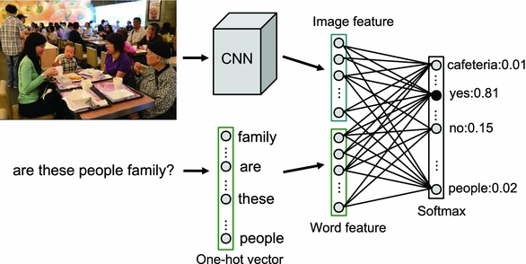
One well-known baseline (Zhou et al. Reference Zhou, Tian, Sukhbaatar, Szlam and Fergus2015) proposed a simple model for VQA on the VQA v1 dataset. This model, illustrated in Figure 10, uses a visual representation produced by the last fully-connected/average-pooling output of a CNN, i.e., V ∈ R d × 1, and bag-of-words as the question representation. These image and language representations are then concatenated and the combined feature is sent to a softmax layer to predict the answer class. Note that in this model both the open-ended and multiple-choice tasks are formulated as classification tasks. While simple, the model achieved comparable performance to several more complicated approaches at that time. Improvements over this baseline used RNN (Antol et al. Reference Antol, Agrawal, Lu, Mitchell, Batra, Zitnick and Parikh2015; Malinowski, Rohrbach and Fritz Reference Malinowski, Rohrbach and Fritz2015; Ren et al. Reference Ren, Kiros and Zemel2015a) or a language CNN (Ma, Lu and Li Reference Ma, Lu and Li2016) to model the question (and answer).
Image-based VQA Baseline model used in (Zhou et al. Reference Zhou, Tian, Sukhbaatar, Szlam and Fergus2015).

Attention Models: Since then, most research has focused on modeling the interaction between image content and question for improving performance, as well as on model interpretability. In many cases, an answer only relates to a small portion of the image, e.g. the answer to the question What is the color of the boy’s shirt? given an image containing a boy and a cat, only relates to the boy. Thus, using global image features to predict the correct answer usually leads to suboptimal results due to noisy information introduced by the irrelevant image regions.
To address this issue, recent models (Yang et al. Reference Yang, He, Gao, Deng and Smola2016; Xiong, Merity and Socher Reference Xiong, Merity and Socher2016; Xu and Saenko Reference Xu and Saenko2016; Shih, Singh and Hoiem Reference Shih, Singh and Hoiem2016; Chen et al. Reference Chen, Wang, Chen, Gao, Xu and Nevatia2015b; Das et al. Reference Das, Agrawal, Zitnick, Parikh and Batra2017; Selvaraju et al. Reference Selvaraju, Cogswell, Das, Vedantam, Parikh and Batra2017) examine different spatial regions within the image and compare their contents (and locations) to help in answering visual questions. Rather than extracting a single feature for the whole image, these models compute visual representations consisting of the last convolutional output V ∈ R d × G, where d is the feature dimension and G is the number of spatial grids. These are fed through a single layer neural network and then a softmax function generates an attention distribution over image regions:
 $$\begin{equation}
\begin{split} q &= \mbox{LSTM}(Q) \\
H_v &= \mbox{tanh}(W_v V + W_q q)\\
a^v &= \mbox{softmax}(w_{h,v}^T H_v) \\
\end{split}
\end{equation}$$
 $\widetilde{v}$ guided by the question is computed as
 $\widetilde{v} = \sum _{i=1}^{G} a^v_i v_i$
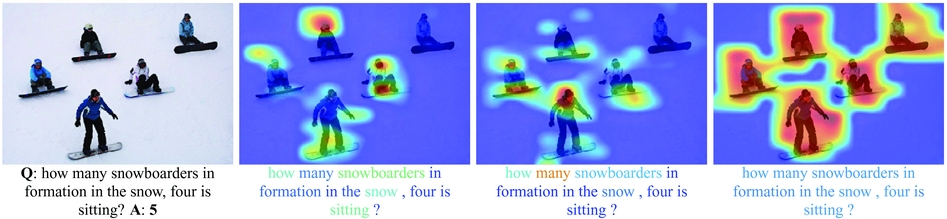
In addition to modeling ‘where to look’ through visual attention, it can also be useful to model ‘what words to listen to’ (Nam, Ha and Kim Reference Nam, Ha and Kim2017; Lu et al. Reference Lu, Yang, Batra and Parikh2016). A co-attention model has been proposed (Lu et al. Reference Lu, Yang, Batra and Parikh2016) that jointly reasons about question-guided visual attention and image-guided question attention. This model co-attends to the image and question in a hierarchical structure over word-level, phrase-level, and question-level embeddings. Given the embedding E = {e t|t = 1, . . ., T} for the input question words Q and the question-guided visual representation  $\widetilde{v}$, the image-guided question representation is computed as
 $$\begin{equation}
\begin{split} H_q &= \mbox{tanh} (W_e E + W_v \widetilde{v})\\
a^q &= \mbox{softmax}(w_{h,q}^T H_q)\\
\widetilde{q}^w &= \sum _{t=1}^{T} a^q_t e_t\\
\end{split}
\end{equation}$$
Visualization of image and question co-attention maps in (Lu et al. Reference Lu, Yang, Batra and Parikh2016). From left to right: original image and question pairs, word-level co-attention maps, phrase-level co-attention maps, question-level co-attention maps. The attentions are scaled from red:high to blue:low.

While most of the above work used concatenations, element-wise products or sums for interactions between the visual and textual representations, Multimodel Compact Bilinear pooling (MCB) (Fukui et al. Reference Fukui, Park, Yang, Rohrbach, Darrell and Rohrbach2016) is an alternative solution for cross-modality interaction. MCB pooling projects an outer product to a lower dimensional space and avoids computing the outer product directly. Fukui et al.’s model uses MCB twice, once to predict spatial attention and once to predict the answer, achieving state-of-art results in 2016.
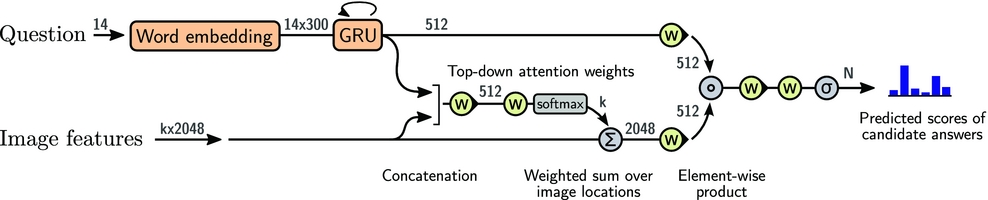
Most recently, the winning model of the 2017 VQA Challenge was a bottom-up and top-down attention model (Anderson et al. Reference Anderson, He, Buehler, Teney, Johnson, Gould and Zhang2017). The authors argued that a uniform grid of equally sized and shaped receptive fields—irrespective of the content of the image—as usually used in attention models, is suboptimal. Instead, their bottom-up mechanism proposes a set of detected image regions for consideration, with each region represented by a pooled convolutional feature vector. These bottom-up regions are detected by Faster R-CNN (Ren et al. Reference Ren, He, Girshick and Sun2015b); a top-down mechanism then uses task-specific context to predict an attention distribution over the proposed image regions. The full VQA model is shown in Figure 12.
Model proposed by (Anderson et al. Reference Anderson, He, Buehler, Teney, Johnson, Gould and Zhang2017).

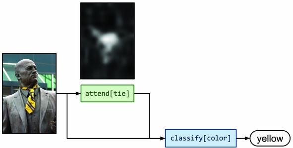
Modular Networks: The first module network for question answering was proposed in 2016 (Andreas et al. Reference Andreas, Rohrbach, Darrell and Klein2016a) and later extended to VQA (Andreas et al. Reference Andreas, Rohrbach, Darrell and Klein2016b). Neural module networks (NMN) approach the VQA task by dynamically composing networks of independent neural modules, jointly trained. Modules are selected based on a parse of the question to utilize only modules that are relevant to the particular question content. Specifically, the authors define the following modules: [COMP: Please insert bracket around display list item, that is, 1., 2. . .. should be changed to (1), (2). . .]
1. Attention module attend[c] performs Image → Attention to spatially select mentioned objects c.
2. Re-attention module re-attend[c] takes an attention heatmap and maps it to another attention, i.e. Attention → Attention.
3. Combination module combined[c] merges two attentions into a single attention, i.e. Attention × Attention → Attention.
4. Classification module classify[c] takes an attention and image then maps them to a distribution over labels, i.e. Image × Attention → Label.
5. Measurement module measure[c] takes an attention and maps it to a distribution over labels, i.e. Attention → Label.
Given a question, modules are selected based on a language parser (De Marneffe et al. Reference De Marneffe2006), and are then mapped to a network structure assembling the relevant modules (see Figure 13 for an example). Given the question ‘What color is his tie?’, NMN generates its composition of  $\texttt {classify[color](attend[tie])}$, the answer coming from the final classification module for color labels. This strategy takes advantage of the inherently compositional property of language, and inspired further work on visual reasoning (Johnson et al. Reference Johnson, Hariharan, van der Maaten, Hoffman, Fei-Fei, Zitnick and Girshick2017b; Hu et al. Reference Hu, Andreas, Rohrbach, Darrell and Saenko2017).
NMN for answering ‘What color is his tie?’ by Andreas et al. (Reference Andreas, Rohrbach, Darrell and Klein2016b).

4.2 VQA in video
4.2.1 Video-based QA datasets
TGIF-QA (Jang et al. Reference Jang, Song, Yu, Kim and Kim2017) This dataset consists of QA pairs on animated GIFs, collected using predefined templates. The QA pairs include three tasks: (1) counting the number of repetitions of a given action, (2) detecting a repeated action given its count, and (3) identifying state transitions, i.e. what happened before or after a specified action state. For example, ‘Q: What does the duck do 3 times?, A: Shake head’. In addition, the authors also generate Frame-QAs for object/number/color/location questions that are answered by one of the frames.
LSMDC-QA (Maharaj et al. Reference Maharaj, Ballas, Rohrbach, Courville and Pal2017) is built on LSMDC (Rohrbach et al. Reference Rohrbach, Rohrbach, Tandon and Schiele2015), a dataset for movie description. To construct this dataset, the authors recast the video description problem as a fill-in-the-blank question-answering task. Given a video and its description with one word blanked-out, the goal is to predict the missing word, e.g. ‘Q: She opens the [blank]. A: door’. The blanked words cover entities, actions and attributes, requiring models to understand the visual content of videos. Since each fill-in the blank answer is a single word evaluation is simple.
VideoQA (Zhu et al. Reference Zhu, Xu, Yang and Hauptmann2015) The videos used in this dataset are from TACoS Multilevel (Regneri et al. Reference Regneri, Rohrbach, Wetzel, Thater, Schiele and Pinkal2013) cooking dataset, MPII-MD (Rohrbach et al. Reference Rohrbach, Rohrbach, Tandon and Schiele2015) movie description dataset, and TRECVID MEDTest (Over et al. Reference Over, Fiscus, Sanders, Joy, Michel, Awad, Smeaton, Kraaij and Quénot2014) web videos. The authors generate three types of QA pairs from their associated descriptions: Inferring the past, Describing the present, and Predicting the future. For each description, some phrase or words are blanked out, which are used to answer the three types of questions, e.g. ‘Q: Predict the future. He [blank] cucumber on plate. A: places’. There are four candidate fill-in-the-blank answers, where only one is correct, a simple multiple-choice evaluation.
MovieQA (Tapaswi et al. Reference Tapaswi, Zhu, Stiefelhagen, Torralba, Urtasun and Fidler2016) This dataset contains more diverse sources of information compared with the other video-based VQA datasets, including plot synopses, videos, subtitles, DVS, and scripts. Here, the authors use plot synopses to collect questions about movies. During data collection, each annotator is shown a paragraph from a plot synopsis then asked to provide questions and answers related to the provided plot. This often results in complex high-level questions that require a great deal of understanding to answer. For, example, ‘Why does Cypher betray Morpheus?’ in the Matrix movie. Multiple-choice is used for evaluation. The whole dataset contains 408 movies and 14,944 QAs, but only 140 videos have video to plot alignment, resulting in 16,066 video clips (Table 5).
Video question answering datasets information including number of question–answer pairs, number of videos, average video length and source domain

PororoQA (Kim et al. Reference Kim, Heo, Choi and Zhang2017) Different from above, the media domain of PororoQA is cartoons, sampled from the popular children’s series ‘Pororo’. This show has a simple, clear, and coherent story structure and a small environment compared to dramas or movies. Each of the 16,066 video clips contain dialogs and each clip is short (thirty-four frames). All questions and answers were written by people and evaluation is multiple-choice question answering, where each question is coupled with five possible answers (one correct and four incorrect). This dataset allows for reasoning about characters that carry over the whole dataset, e.g. ‘Q: What does Pororo think when he hides behind the tree? A: Pororo thinks Loopy can’t find him’.
MarioQA (Mun et al. Reference Mun, Seo, Jung and Han2017) MarioQA is a synthetic video QA dataset, constructed on Super Mario Bros gameplay videos. Questions are synthesized using templates, asking about event-centric questions, counting questions, and state questions, e.g. ‘Q: What enemy did Mario kill by stomping?, A: Para Goomba’. These questions are split into different levels of reasoning complexity: questions without temporal relationships (NT), questions with easy temporal relationships (ET), and questions with hard temporal relationships (HT). These event-centric questions are especially suited to evaluate the temporal reasoning capability of algorithms.
4.2.2 Video-QA models
Frame representation: Each video is composed of a set of frames F = {F 1, F 2, . . ., F N}. Similar to image-based VQA models, CNNs are typically used for extracting visual representations. We denote each frame feature as F n = {f n, i|i = 1, . . ., G}, where n denotes the nth frame and G is the number of regions. Note, the frame feature here is not restricted to CNN features on RGB images. Some recent works also consider using optical flow or spatial-temporal features via C3D (Hendricks et al. Reference Hendricks, Wang, Shechtman, Sivic, Darrell and Russell2017; Jang et al. Reference Jang, Song, Yu, Kim and Kim2017, Reference Jang, Song, Yu, Kim and Kim2017).
The simplest way to abstract the representation of each F n is via mean pooling. Additionally, spatial attention models can be used to learn which regions of F n to attend to for a given question Q. The spatial attention score for each region can be computed as (Yu et al. Reference Yu, Ko, Choi and Kim2016b; Jang et al. Reference Jang, Song, Yu, Kim and Kim2017; Zhao et al. Reference Zhao, Yang, Cai, He and Zhuang2017):
 $$\begin{equation}
s_{ni} = w \mbox{tanh}(W_{qs}q + W_{fs}f_{ni}+b_s)
\end{equation}$$
 $\alpha _{ni} = \frac{\mbox{exp}(s_{ni})}{\sum _i \mbox{exp}(s_{ni})}$, where q = LSTM(Q) is the question feature as in Eq. (5). Then, the spatially attended visual representation for each frame is computed as v n = ∑iαnif ni.
Video representation: Given frame features (with or without attention), the next step is to encode the whole video. One method uses mean-pooling, f n (Venugopalan et al. Reference Venugopalan, Xu, Donahue, Rohrbach, Mooney and Saenko2015)  $\widetilde{v}=\frac{1}{N}\sum _n f_n$, as the final video representation, but this weights the importance of each frame equally ignoring information about what portion of the video the question focuses on. Some authors (Yu et al. Reference Yu, Ko, Choi and Kim2016b; Zhao et al. Reference Zhao, Yang, Cai, He and Zhuang2017; Jang et al. Reference Jang, Song, Yu, Kim and Kim2017) model video as a temporal sequence and use an RNN to encode its information. For example, if we use an LSTM to encode the video, then a corresponding sequence of hidden states
 $\widetilde{v}=h_N$ can be computed as (Yu et al. Reference Yu, Ko, Choi and Kim2016b): h n = LSTM(v n, h n − 1). The final output is then the final video representation
 $\widetilde{v}$.
In addition to spatial attention, temporal attention can also play an important role for localizing what portion of the video content is useful for answering a given question. Zhao et al. (Reference Zhao, Yang, Cai, He and Zhuang2017) and Jang et al. (Reference Jang, Song, Yu, Kim and Kim2017) consider applying a temporal attention model, computing the relevance scores over each hidden state h n:
 $$\begin{equation}
s^{(t)}_n = w^{(t)}\mbox{tanh}(W_{qt}q + W_{ht} h_t + b_t)
\end{equation}$$
 $$\begin{equation}
\beta _n = \frac{\mbox{exp}(s^{(t)}_n)}{\sum _n \mbox{exp}(s^{(t)}_n)}
\end{equation}$$
 $\widetilde{v}=\sum _n \beta _n h_n$ is regarded as a question-driven video representation.
Question answering: Similar to image-based QA, the inference model depends on the type of question–answer pairs. As in image-based VQA, for the open-ended question-answering task the model is formulated as a generation/classification model producing a sentence answer, while for multiple-choice QAs a classification model is typically used. Taking the classification model as an example, given the video representation  $\widetilde{v}$ and question representation q, one approach is to first fuse the video and question modalities (Jang et al. Reference Jang, Song, Yu, Kim and Kim2017):
 $\widetilde{v}_q = \mbox{tanh}(W_v\widetilde{v}) \oplus q$, where ⊕ is an element-wise sum and W v is a transformation matrix to make the dimensions of the two modalities equal. A linear classifier can be defined that takes as input the video-question vector
 $\widetilde{v}_q$, computing the confidence score for the cth answer as
 $\mbox{s}_c = \mbox{softmax}(W_c \widetilde{v}_q + b_c)$, where W c and b c are model parameters. At inference time, the solution is simply selected as c* = argmaxc ∈ Csc.
5 Conclusion
We have reviewed recent work in language and vision tasks, including datasets and methods for producing general natural language descriptions of images (Section 2), referring expression generation and comprehension (Section 3), and visual questions answering (Section 4). There has been a great deal of progress on each of these tasks, largely due to the growing availability of large labeled datasets and neural learning based methods. Moving forward, we foresee vision and language tasks moving into the real world where intelligent agents collaborate and communicate with people. This implies a need for algorithms that can produce not just static language about fixed physical objects and scenes, but also adaptively interact with people through dialog and exploration. As a result, there will be new data and evaluation challenges that will be exciting to investigate.