Victorian Britain

Nineteenth century England is famous for the “dark satanic mills” that were spawned by the industrial revolution. By mid-century smoke pollution in industrial towns had risen to unprecedented levels. Friedrich Engels (Reference Engels1892, p. 40) reported of Bradford in the 1840s that “on week-days the town is enveloped in a grey cloud of coal smoke, but on a fine Sunday it offers a superb picture, when viewed from the surrounding heights.” In 1888 a correspondent of the Manchester Guardian noted that: “Our city, which ought to be one of the finest in the kingdom is to be entirely at the mercy of the smoke and noxious vapour producer, with the result that the atmosphere is poisonous, mortality at its highest rate, and altogether produces the most depressing effect upon the spirits of those unfortunate inhabitants who are compelled to live within its boundaries” (quoted in Mosely Reference Mosley2008, p. 15). Smoke pollution was pervasive even in less heavily industrialized cities like York, where emissions from railway works and the local iron foundry blackened and eroded the walls of the Minster (Brimblecombe and Bowler Reference Brimblecombe and Bowler1992).Footnote ²

The smoke emitted by industry was exacerbated by the use of coal for domestic heating and cooking, which accounted for about one-fifth of inland coal use (Mitchell Reference Mitchell1984, p. 12). The effects were compounded by the crowded conditions in the industrial towns with their back-to-back terraces and crowded tenements, often without trees. These conditions are exemplified by the periodic smogs that occurred typically in cold, humid, and still conditions, associated with anticyclones and temperature inversions. The famous London smogs produced excess mortality especially from bronchitis and pneumonia (Clay and Troesken Reference Clay and Troesken2011). Such conditions were common to most towns but, for a given population density, they were made much worse by the emissions from concentrations of heavy industry.

Total coal consumption (excluding overseas shipments and bunkers) increased more than tenfold during the nineteenth century. In Manchester the number of factory chimneys increased from 500 in the 1840s to around 2,000 at the end of the century (Mosely Reference Mosley2008, pp. 129, 147). Pollution worsened in step with the growth of coal consumption and faced little effective regulation until the end of the century (Wohl Reference Wohl1983, pp. 220–24; Thorsheim Reference Thorsheim2006, pp. 114–24; Mosely Reference Mosley2008, pp. 173–80; Clay and Troesken Reference Clay and Troesken2011).Footnote ³ Coal consumption peaked in the 1950s and has since fallen by nearly 80 percent, while increasing regulation has reduced emissions even more steeply. In 1922 emissions of black smoke were 50 times greater than they were 80 years later (Air Quality Expert Group 2005, p. 263). Indirect measurements for London and Glasgow suggest even greater reductions since the late nineteenth century (Harrison Reference Harrison2006; Aplin Reference Aplin2012).Footnote ⁴

Despite the seemingly obvious importance of atmospheric pollution, the debate over environmental health in the nineteenth century has focused chiefly on the inadequacies of water supply and sewage systems in densely populated towns. A number of studies have found that sanitary reforms were important in reducing infant mortality in the United States (Cain and Rotella Reference Cain and Rotella2001; Troesken Reference Troesken2002; Cutler and Miller Reference Cutler and Miller2005). However, in their examination of 36 English towns between 1871 and 1905, Robert Millward and Frances Bell (Reference Millward and Bell1998) found that while growth in incomes, implying better nutrition, and improvements in housing had substantial influences on the reduction in mortality, investment in sanitation had only modest effects. In contrast, Jonathan Chapman (Reference Chapman2016) estimates the effect of investment in sanitary infrastructure on mortality rates in 381 urban districts from 1861–1870 to 1891–1900 and finds that these improvements significantly reduced mortality rates, especially in the under-five age group. Growth in the stock of sanitation-related capital accounts for between 15 and 25 percent of the overall mortality decline of about one-fifth between 1861–1870 and 1891–1900.

In contrast to the debate over the effects of better nutrition versus sanitary improvements, the effects of atmospheric pollution have received much less attention. As noted by Simon Szreter (Reference Szreter2005, p. 126) “clean air was one obvious omission from the late nineteenth century sanitary arsenal.” Partly as a result of this, there are few direct measurements of air pollution to correlate with health outcomes. However, in recent articles Hanlon (Reference Hanlon2016) and Beach and Hanlon (Reference Beach and Hanlon2018) develop a proxy for industrial pollution using the industrial structure of employment in different registration districts to estimate coal use. They find that this measure of coal use has a strong positive correlation with mortality for a cross-section of registration districts in the decade 1851–1860, and especially with mortality from diseases of the respiratory system. They estimate that pollution accounts for about one-third of the urban mortality penalty, with the greatest impact on children under five years old. Beach and Hanlon’s findings suggest that atmospheric pollution was a major health hazard but, as with much of the debate over sanitation, the focus is on death rates and the causes of death. Yet, exposure to atmospheric pollution also has long-term consequences for those that survive.

Literature on the Links between Pollution and Health

A large medical literature has identified the threats to health arising from atmospheric pollution. Black smoke is emitted from combustion of fossil fuels such as coal as well as petroleum oil, natural gas, and other biomass fuels. It contains carbon dioxide (CO₂), sulphur dioxide (SO₂), and nitrogen oxides (NOx). These combine with moisture and solid material in the atmosphere, through primary and secondary reactions, to form suspended particulate matter with different degrees of fineness. Fine particulate matter is particularly damaging as it also contains substances such as acid sulphates and trace metals and it can more easily be absorbed into the respiratory system. The effects are particularly strong during childhood, as children are more vulnerable during the process of physical development and they may have greater exposure by spending more time outdoors. The resulting inflammation of the lungs and oxidative stress leads to bronchitis and asthma, the effects of which may be greater for those with pre-existing illnesses (Schwartz Reference Schwartz2004; Bateson and Schwartz Reference Bateson and Schwartz2008; Anderson Reference Anderson2009).

Recent research on the effects of atmospheric pollution has identified significant negative effects on the health of children, both concurrently and in later life (for a useful survey see Currie et al. Reference Currie, Graff Zivin, Mullins and Neidell2014). Most of the existing literature focuses on the modern era (since 1950). Such studies have investigated the effects on health of a variety of pollutants, notably vehicle emissions, atmospheric lead, the effects of the Chernobyl nuclear disaster, and even pollen concentrations (Almond, Edlund, and Palme Reference Almond, Edlund and Palme2009; Nilsson Reference Nilsson2009; Currie and Neidell Reference Currie and Neidell2005; Marcotte Reference Marcotte2016). These pollutants have been associated with negative effects on a range of child outcomes, such as infant and child mortality rates, cognitive ability, educational attainment, as well as adult outcomes such as productivity, earnings, and later-life morbidity. In a recent article Vellore Arthi (Reference Arthi2018) examined the long-term effects of exposure to the dust bowl of the 1930s. Using the U.S. censuses for 1980–2000 she finds that exposure led to lower college completion, higher incidence of disability and dependence, and poverty.

Here the focus is on coal combustion, which when concentrated, produces a particularly toxic form of pollution. Several studies have analysed its effects. Karen Clay, Joshua Lewis, and Edson Severnini (Reference Clay, Lewis and Severnini2016) studied the effects of the installation of coal-fired electricity generating plants in the United States between 1930 and 1962, finding that this increased local infant mortality within a 30-mile radius by 5–7 percent. Michael Ransom and C. Arden Pope (Reference Ransom and Pope1995) examined the local effect of the shutting down and reopening of a steel mill in Utah in the 1980s. The effects were large and immediate: hospital admissions of pre-school children on account of asthma and bronchitis were halved when the plant was not in operation. There is also evidence that the introduction of clean air acts in the United States reduced infant mortality and increased earnings in later life (Chay and Greenstone Reference Chay and Greenstone2003; Isen, Rossin-Slater, and Walker Reference Isen, Rossin-Slater and Walker2017). At the same time, even low (post-legislation) levels of emissions have discernible effects on deaths from respiratory and cardiovascular disease in the United Kingdom (Janke, Propper, and Henderson Reference Janke, Propper and Henderson2009).

Emissions in developing countries are more comparable with historical levels, and the evidence suggests that these have substantial effects on mortality. Seema Jayachandran (Reference Jayachandran2009) finds that smoke from the massive 1997 wildfires in Indonesia increased the mortality rate of children under the age of three by 20 percent. Similarly, Shinsuke Tanaka (Reference Tanaka2015) finds that restrictions placed on the emissions of coal fired powers stations in China in 1997 reduced infant mortality by 20 percent in the prefectures in which the policy was applied. In Turkey the progressive replacement of coal by natural gas for cooking and heating also had substantial effects, reducing infant mortality by around 30 percent over the decade 2001 to 2011 (Cesur et al. Reference Cesur, Tekin and Ulker2017).

Most studies relate to outcomes such as mortality among different age groups but there are longer-term effects of exposure on those who survive. Medical studies identify the effects of particulate matter (PM₁₀ or PM_2.5) on pulmonary function and lung development through oxidative stress, which leads to inflammation and often to acute and repeated respiratory symptoms (Heinrich and Slama Reference Heinrich and Slama2007; Rückerl et al. Reference Rückerl, Schneider and Breitner2011).Footnote ⁵ Inhalation of ultrafine particles that penetrate the lung surface lining (epithelium) enter the bloodstream, facilitating the translocation of particles to other organs. These pathways retard growth by diverting the body’s energy to fighting disease rather than building bone and muscle.

Studies of developing countries find that stunting is much more common among young children in households that rely on biofuels than among those in households using cleaner fuels (Mishra and Retherford Reference Mishra and Retherford2007; Kyu, Georgiades, and Boyle Reference Kyu, Georgiades and Boyle2009; Ghosh et al. Reference Ghosh, Amirian, Dostal and Sram2011). The effects of ambient air pollution on height are more difficult to assess. One study found that children residing in the highly polluted center of Krakow grew by 1.5 cm less over two years than those less exposed (Jedrychowski, Maugeri, and Jedrychowska-Bianchi Reference Jedrychowski, Maugeri and Jedrychowska-Bianchi2002). For the United Kingdom, Martin Bobak, Marcus Richards, and Michael Wadsworth (Reference Bobak, Richards and Wadsworth2004) examined heights in a cohort study of children born in one week in 1946, a time when coal consumption was still relatively high.Footnote ⁶ They found a negative relationship between coal consumption and height at years of age between 2 and 7. This result was robust to the inclusion of birth-weight, suggesting that the effects were not principally in utero.

In the light of these results one might expect significant effects of atmospheric pollution on health in late nineteenth century Britain. Indeed, Hanlon and Yuan Tian (Reference Hanlon and Tian2015) find that the mortality gradient between less and more polluted areas was steeper in late-nineteenth century Britain than in modern China. In what follows we explore the question of whether, and to what extent, coal use affected growth during childhood, as reflected in the adult heights of those born in the 1890s. Our focus on individuals also has the advantage that it avoids the potential ecological fallacy of inferring individual effects from group-level analysis.

Estimating Framework

To examine the effects of atmospheric pollution on the health and growth of children in nineteenth century Britain we use a sample of the heights of servicemen born in the 1890s who enlisted in the British army during WWI. We link them to the households and localities in which the servicemen grew up, as observed in the 1901 census. By using the heights of young adults, we are able to assess the longer-term effect of exposure to pollutants during the individual’s childhood. Our estimating framework can be represented as follows:

(1) ${H_{ij}} = {\alpha _1}{A_{ij}} + {\alpha _2}{C_j} + {\alpha _3}{F_{ij}} + {\alpha _4}{L_j} + {e_{ij}},$

where H_ij is the height on enlistment of serviceman i who grew up in locality j. A_ij is the serviceman’s age on enlistment and C_j is a measure of the coal intensity of the district of residence in 1901, our chief variable of interest. F_ij is a vector of household variables as observed during childhood in 1901, and L_j is a vector of other characteristics of the locality, both sets included as controls; e_ij is an unobserved mean-zero random error, assumed to be uncorrelated with the explanatory variables.

Army Service Records

We select our sample from the army service records that have been made available on Ancestry.co.uk. The army service records originate from the file WO363 held in the National Archives, which contains the records of around two million servicemen who completed their army service between 1914 and the early 1920s. These records comprise a (not necessarily complete) set of forms for each serviceman. The information that we use is taken from the attestation form completed at enlistment and the medical inspection report form. The attestation form records name, age, address, and usually the serviceman’s birthplace and details of his next of kin. The medical inspection report records various physical characteristics relating to fitness for service and, most importantly, height in inches. A sample was taken of the first 2 percent of each three-letter combination for about one-third of the letter combinations,Footnote ⁷ the principal focus being on those born between the years 1892 to 1897. In total we have records for 2,956 servicemen.

Using a sample from WWI mitigates possible concerns about selection into the army.Footnote ⁸ Recruitment to the British army was not very selective and it included a large proportion of the relevant cohorts of adult males. It is estimated that 46 percent of males aged 15–49 in England and Wales in 1911 were recruited into the armed forces (Winter Reference Winter2004, p. 28). We focus on men born in the 1890s of whom about two-thirds served in the war.Footnote ⁹ The sample includes both volunteers, most of whom enlisted in the early years of the war, and those who entered the army after the introduction of conscription in March 1916.Footnote ¹⁰ For these reasons alone, those who enlisted were fairly representative of this cohort of men. Nevertheless, the results presented below apply only to those selected into the army.

One particular concern in samples of army recruits is the minimum height requirement. The height standard, which was five feet three inches at the beginning of the war was reduced to five feet two in May 1915.Footnote ¹¹ In November 1914 the first Bantam regiments were formed, for which the minimum height was four feet ten inches. Even though recruits were subject to medical examinations, these were notoriously superficial and the rejection rate declined as the pressure for recruits mounted. By the last year of the war, when a large proportion of those fit for service had already enlisted, just 10 percent of those examined were rejected as unfit for any kind of service (Winter Reference Winter2004, p. 57). Only a very small proportion of these were rejected on the grounds of “poor physique,” although the medical grounds for rejection could well have been correlated with height.Footnote ¹² So it is likely that those with very poor health, and perhaps with unusually short stature, are underrepresented. On the other hand, the army service records do not include those that entered the army as commissioned officers. These were selected from the middle and upper classes and were typically taller than average. Of those who served in the army about 5 percent were officers, although many of these would have risen from the ranks. Overall it is likely that the army service records somewhat under-represent the extreme tails of the underlying height distribution.

The individual’s childhood circumstances are captured by finding each serviceman in the 1901 census of England and Wales. We discard those that were resident in Scotland or Ireland and those for whom key information is missing from the service record. We search by name and age-range and then use other information in the army service records to discriminate between alternative potential matches.Footnote ¹³ One important aid to identifying the correct household is that most servicemen were unmarried at the time of enlistment; their next of kin reported at enlistment was usually a parent who would be observed in the same household in 1901. We discard cases for which no match was found, or where there was no basis to choose among alternatives. We further discard those who turned out not to be born in the 1890s or who were living in institutions containing more than 15 people. Our final matched sample consists of 2,235 individuals.

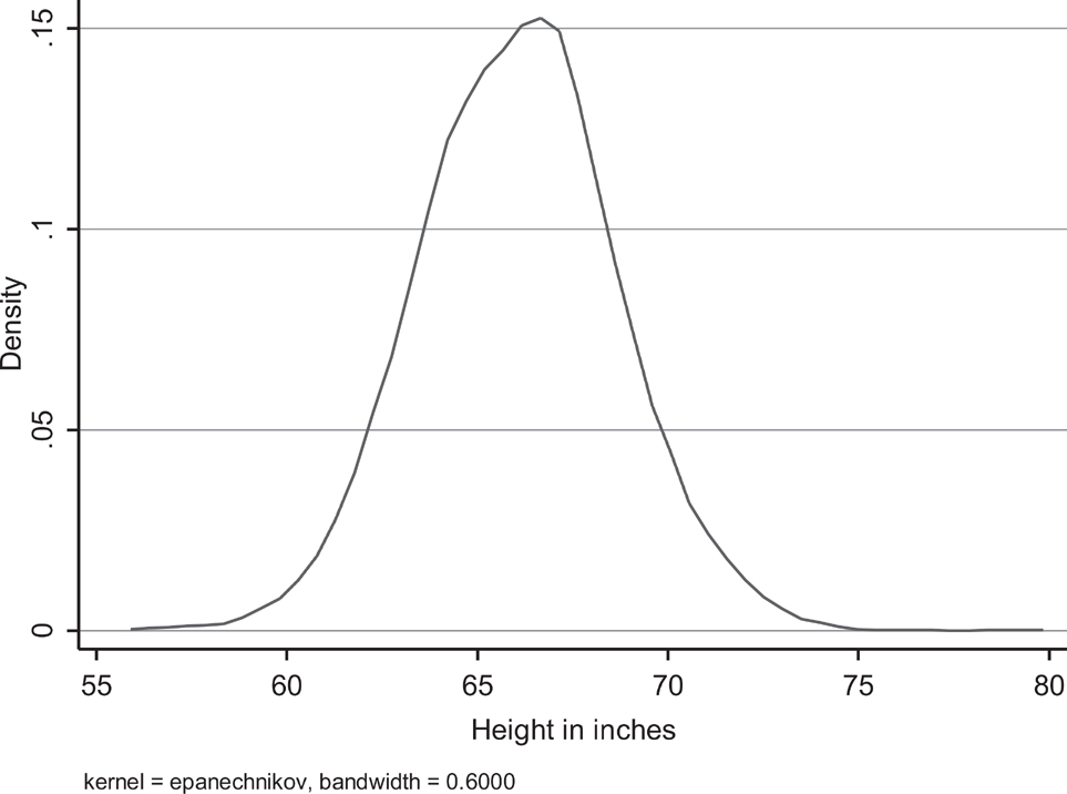
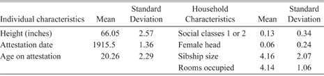
The distribution of heights in our sample of servicemen is shown in Figure 1. The average height is five feet six inches, although the modal height is five feet seven. Although normality can be rejected the tails of the distribution are fairly symmetrical, with 9.5 percent of the sample shorter than five feet three inches and 10.8 percent taller than five feet nine inches. Some mean characteristics of these individuals are reported in the left-hand panel of Table 1. The average age of the servicemen was just over 20 on enlistment and the average date of attestation was halfway through 1915.

Figure 1

Kernel Density of Height

Source: Constructed from data described in the text.

Table 1

Individual and Household Characteristics of the Sample of Servicemen

Source: See the text.

Household Characteristics

Most households in which the servicemen were observed as children in 1901 were headed by manual workers, with only 13 percent in white-collar occupations, as represented by social classes 1 and 2. As there was no occupation-based social classification in the 1901 census, this is based on applying the 1921 classification to the occupational titles. The overwhelming majority of the servicemen grew up in male-headed households with the remainder mainly headed by widows. On average each had more than three siblings when observed in 1901. Fertility was still relatively high at the turn of the century and completed sibships would have been larger still. We also have details of the number of rooms occupied which is capped at five. Nearly one-half were living in households with more than one person per room. Other household characteristics are added later as robustness checks for our results. These take the form of indicators of whether the birthplace of the household head or that of the serviceman differed from that recorded in the 1901 census, the purpose being to probe the possible impact of household mobility.

Coal Intensity

The key variable for our purpose is coal use in the locality or registration district in which these servicemen grew up. In 1901 there were 635 registration districts in England and Wales with an average population size of 51,000. The registration districts, based on poor law unions, exhibit a wide diversity of local conditions. We follow Beach and Hanlon (Reference Beach and Hanlon2018) in constructing a measure of coal intensity for each registration district by combining coal use per employee from the 1907 industrial census with the occupational structure of the registration district in the 1901 population census. Our measure of coal intensity for a district can be represented as follows:

(2) $Coal\,{\rm{ }}Intensit{y_j} = \Sigma _{k = 1}^n{c_k}{o_{kj}}/\Sigma _{k = 1}^n{o_{kj}},$

where c_k is annual coal consumption per employee in occupation k, o_kj is the number employed in occupation k in district j, and occupations are indexed from 1 to n. Thus, the ratio is the predicted industrial coal consumption per occupied worker in the registration district.

In order to construct this index, we first link each occupation recorded in the 1901 census to an industry identified in the census of production. These industries represent about 60 percent of inland coal use. The census of production includes 13 industry groups and 139 subgroups for each of which coal consumption per employee is reported.Footnote ¹⁴ We then match the occupations in the 1901 census with these industrial subgroups and give each occupation the coal consumption per employee in the matched subgroup. Only 434 of the 796 unique occupations are matched; the remainder are given a coal consumption value of zero.Footnote ¹⁵ We then obtain average coal consumption in each registration district by applying coal consumption by occupation to the occupational composition of the district. It is important to stress that this is a measure only of industrial coal use. It does not include coal consumed in domestic heating, nor does it cover coal used by railways or coastal shipping. As domestic coal consumption is ubiquitous it should not matter very much for the comparison across districts. And while railways are more concentrated, the atmospheric pollution that they generate would be widely dispersed.Footnote ¹⁶

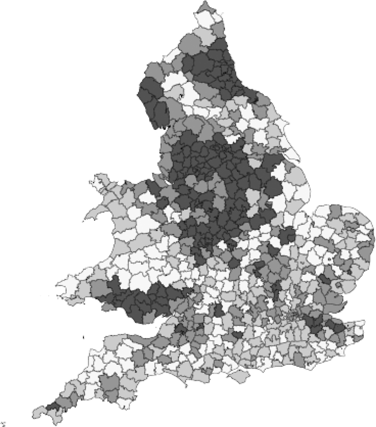
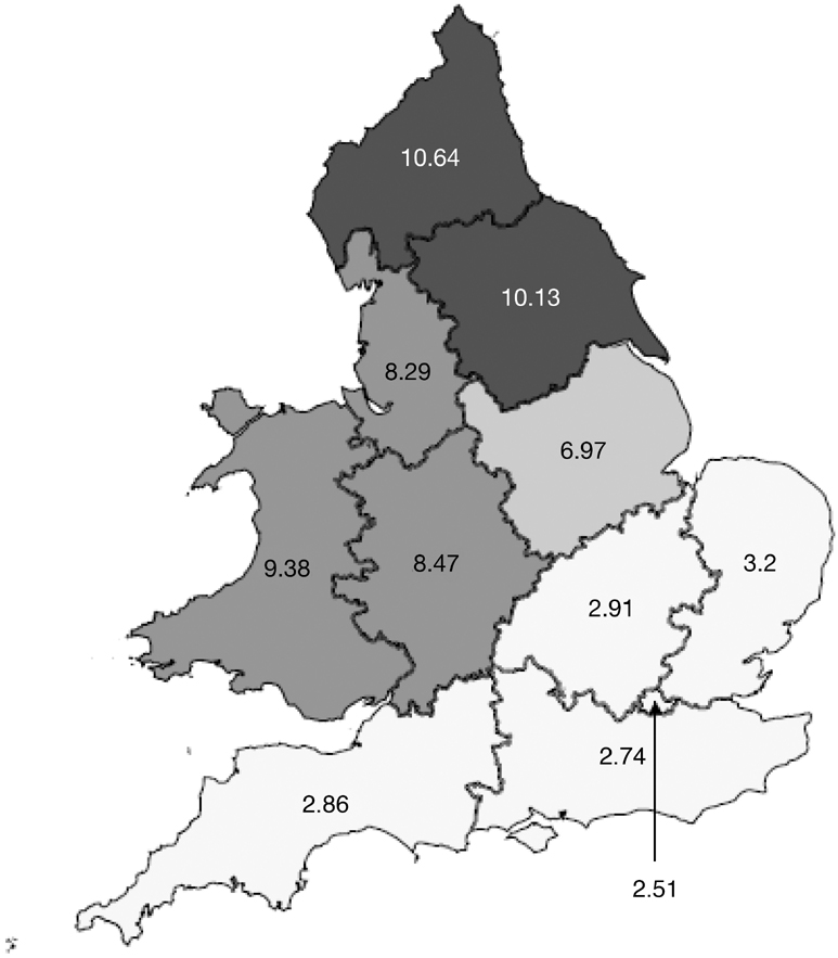
Figure 2 provides a map of the registration districts where darker shading represents higher quartiles of coal intensity. The map highlights the geography of the industrial revolution with a broad swathe of darker shading covering the textile regions of Lancashire and Yorkshire, as well as the manufacturing districts of the midlands and the northwest, and the coal mining areas of the northeast and South Wales. The location of the cotton industry was largely determined by original access to water power, ports, and markets (Crafts and Wolf Reference Crafts and Wolf2014), while heavy industries were located in proximity to minerals, and above all to coalfields (Reference Fernihough and O’RourkeFernihough and O’Rourke 2014). Thus, the distribution of industry owed most to these geographical features and should not be the result of differences in physical stature. The coal intensive districts are highly concentrated in relatively few counties and there are sharp differences between regions. As shown in Figure 3, average coal intensity in the north of England is nearly four times that in the southeast.

Figure 2

Map of Coal Intensity by Registration Districts (Darker for Higher Coal Intensity)

Source: Constructed from data described in the text.

Figure 3

Map of Coal Intensity by Registration Divisions (Darker for Higher Coal Intensity)

Source: Constructed from data described in the text.

We also calculate an alternative measure restricted to heavy coal use. This is represented as:

(3) $Heavy\,{\rm{ }}\,coal\,{\rm{ }}us{e_j} = \Sigma _{k = 1}^n{z_k}{o_{jk}}/\Sigma _{k = 1}^n{o_{jk}},$

where z_k is an indicator that takes the value 1 if the particular occupation is in an industrial subgroup for which coal consumption, c_k , exceeds 10 tons per employee per annum. Heavy coal use concentrates attention on those industries for which the pollution effect is likely to be most severe. It also avoids potential measurement error, which may arise for lower levels of coal intensity.

Locality Characteristics

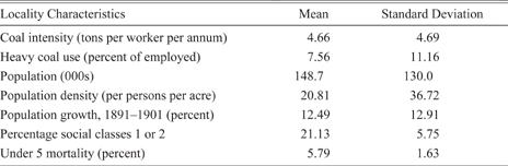
In our sample we observe individuals growing up in 472 out of the 635 registration districts. As Table 2 shows, the average serviceman came from a registration district with a coal intensity of 4.7 tons per worker with 7.6 percent of the labor force engaged in heavy coal use industries. Not surprisingly, these randomly selected individuals are often from the larger registration districts. The average servicemen grew up in a district with a population of nearly 150,000, with a population density of 21 persons per acre, and with population growth of 12.5 percent over the decade 1891–1901. Among the occupied population in the districts, 21 percent were in social classes 1 and 2.

Table 2

Locality Characteristics

Source: See the text.

Additional district-level characteristics are introduced later for different purposes. Wind direction, climate and topography, and lagged coal intensity (estimated from the 1851 census) serve as further robustness checks. Finally, an indicator of the local disease environment—child mortality—is used to explore a possible route by which atmospheric pollution (as measured by coal intensity) may have worsened the local disease environment (as measured by child mortality), and was subsequently reflected in individual servicemen’s adult heights.

Height and Coal Intensity

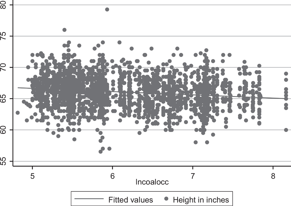
Did coal intensity affect the growth of children in the late nineteenth century and therefore influence their heights as adults? Figure 4 plots height against coal intensity, which is entered in log form to account for the diminishing effect of more intensive coal use.Footnote ¹⁷ Not surprisingly there is a wide scatter of heights with evidence of a mild negative relationship. One might be concerned that the servicemen were selected disproportionately from more (or less) polluted districts. In fact, the share of servicemen from districts with coal intensity above the median is very close to the share of population aged 0 to 9 in these districts. Servicemen from districts with above-median coal intensity are three-quarters of an inch shorter than those from below-median districts (Online Appendix Table A1).

Figure 4

Scatterplot of Height and Log Coal Intensity

Source: Constructed from data described in the text.

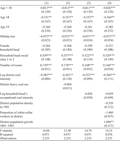
Table 3 reports regression results where the dependent variable is height in inches and the standard errors are clustered by county. The regressions include dummy variables for the 11 divisions of England and Wales shown in Figure 3 (not reported in the table).Footnote ¹⁸ These capture regional differences in climate, such as rainfall, average temperature, and insolation, and possibly also economic differences such as wage and income levels. Thus, our estimates rely on variation within regions.

Table 3

Height and District Coal Intensity

^* = Significant at the 10 percent level.

^** = Significant at the 5 percent level.

^*** = Significant at the 1 percent level.

Note: Robust standard errors, in parentheses, are clustered at the county level. The dependent variable is height in inches. Age in years is taken from the servicemen records, where the reference category is age 20 and over. Household variables, taken from the 1901 census, are: the number of siblings in the family, a dummy = 1 for female household head, a dummy = 1 for the household head in occupation-based social classes 1 or 2, and the number of rooms occupied (capped at 5). The log of district coal intensity and district heavy coal use are constructed from the occupational classification in the 1901 census as indicated in the text. Other district-level variables are: population density (population per 1,000 acres), the proportion of workers in social classes 1 and 2, and the proportional growth of population from 1891 to 1901. Ten regional dummies are included but not reported.

Source: Computed from data described in the text.

The coefficients on individual and household variables are consistent with those reported by Roy Bailey, Timothy Hatton, and Kris Inwood (Reference Bailey, Hatton and Inwood2016) and can be briefly summarized. The dummy variables for year of age show height advancing with age up to 20 after which there is no further increase. The number of siblings is negatively associated with height, which is consistent with the idea of a trade-off between the quality and the quantity of children (a point explored more fully by Hatton Reference Hatton2017). Those who grew up in female-headed households were shorter than those in male-headed households but not significantly so. Not surprisingly, servicemen who grew up in middle class households were about half an inch taller than those in households headed by manual workers. And those growing up in larger dwellings were also taller, by around a third of an inch. The latter two variables, in particular, are strong indicators of income and living standards.

Turning to the principal variables of interest, column (1) shows that our coal intensity variable takes a significant coefficient of −0.285. The coefficient implies that the difference between the 10^th and 90^th percentiles of coal use across registration districts, from 1.6 tons to 11.5 tons per worker, is associated with a difference of more than half an inch in height.Footnote ¹⁹ It is possible that height is only affected by extreme levels of smoke pollution. But as shown in column (2) when the share of the labor force engaged in heavy coal use is added the coefficient is insignificant, while that on coal intensity remains negative and significant. So, the association between coal intensity and child health seems to occur throughout the distribution. This is consistent with the research findings noted earlier that find discernible health effects at relatively low levels of pollution. Clustering standard errors at different levels or allowing for left-side truncation has very little effect on these results (Online Appendix Tables A2 and A3).

It is possible that, in spite of the inclusion of a set of household-level variables, coal intensity may be capturing heterogeneity among households engaged in different industries. Thus, the effect of coal intensity may reflect differences in the composition of household types rather than pure district effects. As pointed out by Edward Higgs (Reference Higgs1991), the Registrar General’s office was much concerned with examining the links between occupations and health outcomes, associating occupation not only with the medical consequences of working with certain materials but also with the individual’s moral and behavioral characteristics.Footnote ²⁰ Thus, if the association between coal intensity and height is to be interpreted as reflecting atmospheric pollution, then it should not be affected by the coal intensity of the household head’s occupation.

In order to test this hypothesis, we linked coal intensity to the occupations of the heads of households of the individual servicemen whom we observe as children in the 1901 census. Coal intensity is zero for 52 percent of our households and so we add one before taking the log. This variable is added in column (3) of Table 3. Although the coefficient is negative it is insignificant. Thus, there is little evidence that those who grew up in households with heads that worked in coal intensive industries suffered worse health than others in the same district. This result indicates that district coal intensity is not simply reflecting the probability that a head of household worked in a coal intensive industry but is a genuine locality effect. It is all the more striking as households with heads engaged in coal intensive industries are likely to have lived nearer to the immediate location of coal combustion than others in the same district.

Another possibility is that coal intensity is capturing other economic features of the district that affect height. We include these in column (4) of Table 3. Population density of the district is often associated with poor sanitary conditions and high death rates. Consistent with this, population density takes a negative coefficient but it is not significant at the conventional level and the magnitude is modest.Footnote ²¹ A further possibility is that districts with a preponderance of occupations with high coal intensity would be predominantly working-class areas with poor infrastructure. Thus, coal intensity may be picking up poor quality social environments rather than specifically reflecting atmospheric pollution. This hypothesis is tested by including the proportion in social classes 1 and 2 in the registration district. The coefficient is negative and insignificant suggesting that our measure of coal intensity is not simply a proxy for the class composition of the district. Finally, the prosperity of the district may be captured by population growth, a view that is supported by the positive coefficient on district population growth from 1891 to 1901. Thus, district population growth of 10 percent over the decade is associated with an increase in height of 0.1 of an inch as compared with a district with a stationary population.Footnote ²² Importantly, the coefficient on coal intensity increases in size and significance in the presence of all these variables.

Wind Direction, Climate, and Topography

If the coal intensity variable captures atmospheric pollution, and especially the presence of particulate matter, then it may have diffused beyond the immediate vicinity and into neighboring districts. As the wind direction is predominantly southwesterly, pollution from outside the district should come from the southwest and not from the northeast. Beach and Hanlon (Reference Beach and Hanlon2018) find that district mortality rates in the 1850s were increased by coal use upwind but not by coal use downwind.Footnote ²³ In order to test this hypothesis we calculate the average coal intensity (as defined in equation (2)) of districts that fall within the southwest quadrant up to 25 km from a central point in the district. The central point in a district is defined either as the major concentration of population (usually a metropolitan district) or, in the case of rural districts, as the approximate geographical center.Footnote ²⁴ The same procedure was used to calculate coal intensity of districts to the northeast and we also calculate variables for heavy coal use in districts to the southwest and to the northeast.

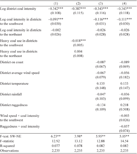
Column (1) of Table 4 shows the result of adding the variables for coal intensity in districts to the southwest and to the northeast. Individual, household, and other locality variables are included but not reported. In column (1) coal intensity to the southwest takes a significant negative coefficient whereas coal intensity to the northeast is insignificant. The F-statistic for the difference between these coefficients is significant at the 5 percent level. In the presence of these variables the coefficient on coal intensity within the district remains negative and significant although it is somewhat smaller than in column (4) of Table 3. This is not surprising in light of the clustering of coal intensity shown in Figure 2. Diffusion across districts might be especially strong where coal use is particularly heavy. Accordingly, column (2) includes the measure of heavy coal use in districts to the southwest and the northeast. Heavy coal use to the southwest takes a negative and significant coefficient while heavy coal use to the northeast does not. These results reinforce confidence in the hypothesis that the coal intensity variables capture atmospheric pollution and not some other effect associated with coal use within each district.

Table 4

Height, Pollution Diffusion, Climate, and Topography

^* = Significant at the 10 percent level.

^** = Significant at the 5 percent level.

^*** = Significant at the 1 percent level.

Note: Robust standard errors, in parentheses, are clustered at the county level. The dependent variable is height in inches. The log of district coal intensity and district heavy coal use are constructed from the occupational classification in the 1901 census as indicated in the text. The analogous variables for the southwest and northeast are calculated for the districts in the respective quadrants at a distance of 25 km. District variables are: a dummy = 1 if on the coast, average wind speed in meters per second in 2000–2010, temperature measured as average annual growing degree days in 1961–1990, rainfall as average daily precipitation in excess of 1 mm, and ruggedness as the average terrain slope. Other controls, not reported, are age dummies for under 18, 18 and 19, number of siblings, a dummy for female head of household, a dummy for head of household in social classes 1 or 2, and the number of rooms occupied (capped at 5). Also included are district level variables for population density (population per 1,000 acres), the proportion of workers in social classes 1 and 2, and the proportional growth of population from 1891 to 1901, as well as ten regional dummies.

Source: Computed from data described in the text.

The association between coal intensity and health and height could also be influenced by topography and climate. Column (3) of Table 4 includes a series of additional district-level variables, each calculated as deviations from its mean. Coastal location and greater wind speed might both be expected to lead to greater dispersal of coal emissions, and hence positive coefficients. The wind speed variable used here is average wind speed (in meters per second) over the years 2000–2010 at a height of 25 meters from the ground (a little higher than most Victorian factory chimneys). This is from the NOABL database of the U.K. Department of Energy and Climate Change. However, both coefficients are negative and neither is significant. Temperature is measured as average annual growing degree days (divided by 365) for 1961 to 1990, taken from the U.K. Meteorological Office’s 5 km gridded database. Higher temperatures could also be associated with greater dispersal of smoke pollution, but while the coefficient is positive it is not significant. Rainfall is measured as average daily precipitation (greater than 1 mm) for 1961–1990, again from the Meteorological Office’s 5 km gridded database. Rainfall could help either to suspend or to disperse particulate matter and the coefficient is negative but insignificant.

Column (3) of Table 4 also includes a measure of terrain ruggedness. This is the average slope in the area of the registration district using elevation data from the Shuttle Radar Topography Mission gridded elevation dataset.Footnote ²⁵ As towns and cities tend to be in valleys rather than on hills, hillier locations may tend to trap atmospheric pollution leading to slower dispersal. The coefficient on ruggedness is negative as predicted but, again, not significant. It is possible also that the effects of climate and geography have interactive effects on health and height and this could account for the lack of significance of some of the coefficients. Column (4) adds two such interactions. One possibility is that the effect of atmospheric pollution in districts to the southwest would increase with higher wind speeds, but the coefficient on the interaction is not significant. Another is that the effect of coal intensity would be greater in hillier locations, but this too gives an insignificant coefficient. It is important to note that adding these additional variables has very little effect on the coefficients on log coal intensity in the district and to the southwest, both of which remain negative and strongly significant.

Migration and Mobility

Although the association of coal intensity with health and height is robust to the inclusion of a range of other variables, the coefficient may still be biased as a result of correlation between coal intensity and other unobserved variables that are also correlated with height. The most obvious source of endogeneity is the selective migration of households into districts with different levels of coal intensity. There was considerable geographic mobility in late nineteenth century (Baines Reference Baines1982; Boyer and Hatton Reference Boyer and Hatton1997; Long Reference Long2005), and it is sometimes argued that migration to the towns and cities selected the fittest. If migrants tended to be taller than average, due to genetic or other reasons, then the same might apply to their children. On the other hand, it is possible that districts with heavy coal use recruited those with below average health, whose children might be shorter than average.Footnote ²⁶ If so then the negative effect of coal intensity on the height of servicemen in our sample could reflect the selective in-migration of their parents.

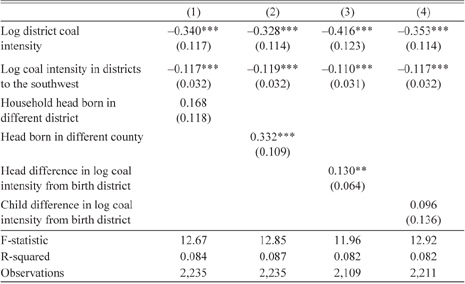
In order to distinguish migrant families, we identify the birthplaces of heads of the households in which the individual servicemen lived as children in 1901. We use the information on birthplaces reported in the census in order to find the county and registration district of birth of the head of household, normally the individual’s father.Footnote ²⁷ Fifty-nine percent of household heads were living in a registration district different from that in which they were born and 36 percent were living in a different county. Column (1) of Table 5 includes a dummy variable taking the value 1 for inter-district in-migrant household heads.

Table 5

Height and Migration

^* = Significant at the 10 percent level.

^** = Significant at the 5 percent level.

^*** = Significant at the 1 percent level.

Note: Robust standard errors, in parentheses, are clustered at the county level. The dependent variable is height in inches. The log of district coal intensity is constructed from the occupational classification in the 1901 census as indicated in the text. The analogous variable for the southwest is calculated for the districts in the quadrant to the southwest at a distance of 25 km. Dummy variables = 1 for birth in a district or county different from residence are from the 1901 census. Differences in log coal intensity between the individual’s district of residence and district of birth (cols. (3) and (4)) are available only for those born in England and Wales. Other controls, not reported, are age dummies for under 18, 18 and 19, number of siblings, a dummy for female head of household, a dummy for head of household in social classes 1 or 2, and the number of rooms occupied (capped at 5). Also included are district level variables for population density (population per 1,000 acres), the proportion of workers in social classes 1 and 2, the proportional growth of population from 1891 to 1901, log coal intensity to the northeast, a coast dummy, average wind speed, annual growing degree days, average precipitation, and ruggedness, as well as ten regional dummies.

Source: Computed from data described in the text.

Individual, household, and locality variables are included, but not reported. The coefficient is positive, but is not significant. Column (2) shows that a dummy for inter-county migrant household heads takes a positive and significant coefficient, equivalent to a third of an inch in height. Positive selection is greater for longer distance moves, which is consistent with what is sometimes called the “healthy migrant effect” (Kennedy et al. Reference Kennedy, Kidd, McDonald and Biddle2015), but in this case for the children of the migrants.

Although the children of migrants were taller as adults than the children of non-migrants, that alone does not identify selection into districts by coal intensity. In order to assess this, we attach the 1901 coal intensity to the district of birth of the head of household. This is only possible for the 94 percent of household heads that were born in England and Wales, for whom we can measure coal intensity in the district of birth. On average, migrant household heads moved to districts where coal intensity was 10 percent higher than in the districts where they were born. Column (3) of Table 5 includes the difference in log coal intensity between the district of residence and the district of birth. The coefficient is positive and significant at the 5 percent level, which suggests that the sons of migrant household heads who moved into districts with greater coal intensity tended to be taller than the average for the district. The coefficient on coal intensity in the district of residence is a little larger in absolute value once we consider the positive selection of households into districts with greater atmospheric pollution from coal. So, the negative coefficient on coal intensity occurs despite, rather than because of, selective in-migration.

The heights of servicemen could also be affected by their own migration during childhood. For those who moved sometime before the 1901 census, childhood exposure to coal pollution would arise partly from the district of residence and partly from the district of birth. This might be especially important in the early years of childhood. In order to examine this issue, we take the individual’s birthplace as recorded in the census and, as with the household heads, we use this to identify the registration district and county of birth. Among the individual servicemen, 21 percent had moved registration district sometime before they were observed as children in the 1901 census and 10 percent had moved county. The average age of the servicemen in 1901 is 5.5 years, which implies that about 4 percent of households moved districts in a year, and 2 percent also moved county. As with the heads of household, we have attached the measure of coal intensity to the individual’s district of birth.

Column (4) of Table 5 includes the difference between the log of coal intensity in the district of residence and that in the district of birth. If coal intensity in the district of birth contributes to height then the coefficient should be positive, representing the contribution of conditions in the district of birth.Footnote ²⁸ Although the coefficient is positive as predicted, it is insignificant. One possible reason is that, in the absence of information on exactly when the individual moved, it is not possible to assign weights for exposure in the district of birth and in the district of residence. Also, as some of these individuals would have moved during the latter years of their childhood (after 1901), there might be some attenuation, although the effects of pollution on height are likely to have been greatest during early childhood. Nevertheless, there is little evidence that the association between coal intensity and height is affected by child migration.

Lagged Coal Intensity

Although we have controlled for a variety of local conditions we might still be concerned that some omitted features of the locality could be correlated with both coal intensity and height. If migration between districts depended on differences in atmospheric pollution then this sorting implies that occupational composition would also be endogenous (Hanlon Reference Hanlon2016; Heblich, Trew, and Zylberberg Reference Heblich, Trew and Zylberberg2016). As an alternative we create a measure of coal intensity by registration district in 1851, almost two generations earlier. This can more plausibly be regarded as exogenous. The spatial pattern of British industrialization was largely established during its first phase and, as noted previously, this was primarily the result of geographical features and geological conditions. Lagged coal intensity is constructed in the same way as in equation (2), but while the industry coal consumption per worker is that from the 1907 census, the occupational distribution to which it is applied comes from the 1851 census.Footnote ²⁹ For registration district j, this variable is defined as:

(4) $Coal\,{\rm{ }}Intensit{y_{j51}} = \Sigma _{k = 1}^n{c_k}{o_{kj51}}/\Sigma _{k = 1}^n{o_{kj51}},$

where c_k is annual coal consumption per employee in occupation k in 1907, o _kj51 is the number employed in occupation k in district j in 1851, and occupations are indexed from 1 to n.Footnote ³⁰

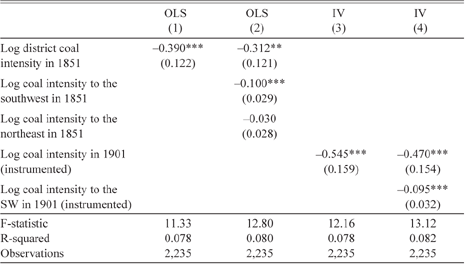
The correlation across localities between this variable and that using the 1901 occupational distribution is 0.75, so the correlation is strong but far from perfect. And the mean is 28 percent lower in 1851 than in 1901 reflecting the earlier stage of industrialization. The result of using this variable in place of the original can be interpreted as a reduced form. The coefficient is reported in column (1) of Table 6, where individual, household, and locality variables are also included but not reported. Log coal intensity in 1851 takes a coefficient which is similar in size and significance to those estimated using the version based on the 1901 occupational distribution. In column (2) we include the log coal intensity to the southwest and to the northeast, both derived from the 1851 occupational distribution. As before, the coefficient on coal intensity to the southwest is significant while coal intensity to the northeast is not, although the difference is only significant at the 10 percent level.

Table 6

Height and Coal Intensity in 1851

^* = Significant at the 10 percent level.

^** = Significant at the 5 percent level.

^*** = Significant at the 1 percent level.

Note: Robust standard errors, in parentheses, are clustered at the county level. The dependent variable is height in inches. The log of district coal intensity in 1851 is constructed from the occupational classification in the 1851 census as indicated in the text for 1901. The analogous variables for the southwest and northeast are calculated for the districts in the respective quadrants at a distance of 25 km. In col. (3) log coal intensity in 1901 is instrumented with log coal intensity in 1851; in col. (4) log coal intensity and log coal intensity to the southwest in 1901 are instrumented with the analogous variables for 1851. Other controls, not reported, are age dummies for under 18, 18 and 19, number of siblings, a dummy for female head of household, a dummy for head of household in social classes 1 or 2, and the number of rooms occupied (capped at 5). Also included are district level variables for population density (population per 1,000 acres), the proportion of workers in social classes 1 and 2, the proportional growth of population from 1891 to 1901, a coast dummy, average wind speed, annual growing degree days, average precipitation, and ruggedness, as well as ten regional dummies.

Source: Computed from data described in the text.

In column (3) we treat log coal intensity in 1901 as endogenous and use log coal intensity in 1851 as the instrument. This gives a coefficient that is nearly one-third larger than the equivalent ordinary least squares (OLS) estimate. This implies a downward bias in the original coefficient, consistent with positive sorting into industrial districts by height, as indicated by the results for in-migrant households in Table 5. Column (4) of Table 6 includes the log of coal intensity to the southwest, where the 1851 equivalent is included as an additional instrument. As before, both variables are negative and significant, adding support for our interpretation of the effect as reflecting atmospheric pollution. Of this estimate about 17 percent of the atmospheric pollution effect comes from neighboring districts. Taking both coefficients into account implies that the difference between 90^th and 10^th percentiles of coal intensity cross servicemen accounts for a difference in height of 1.1 inches.

Causes of Death

The mortality rate among infants or among those under five is widely accepted as a sensitive indicator of the local disease environment as it represents environmental exposure to infections and inflammation (Crimmins and Finch Reference Crimmins and Finch2005). Infant or child mortality in the locality during childhood is often used as an explanatory variable for adult outcomes, including height. Most historical studies find a strong negative relationship with height, consistent with a scarring effect of childhood conditions (Quintana-Domeque, Bozzoli, and Bosch Reference Quintana-Domeque, Bozzoli and Bosch2011; Hatton Reference Hatton2011; Schiman, Kaestner, and Lo Sasso Reference Schiman, Kaestner and Lo Sasso2017).Footnote ³¹ As different causes of mortality will be associated with different elements of the disease environment, distinguishing between causes of mortality should help to identify the epidemiological channels through which the local environment affects height. In particular, if atmospheric pollution is an important influence then we should expect to find a link between height and the incidence of death from respiratory disease.

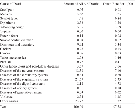
Table 7 shows death rates under the age of five, from specific causes and in total, for England and Wales over the decade 1891–1900. Death rates per thousand are calculated as the annual average of deaths divided by the average population under five years of age. The well-known infectious diseases, measles, scarlet fever, diphtheria, and whooping cough, accounted for 15 percent of all deaths, with another 5 percent accounted for by tuberculosis. Diarrhoea and dysentery, together with other diseases of the digestive system, accounted for nearly 20 percent while respiratory diseases, mainly bronchitis and pneumonia, accounted for 21 percent. Of course, the classification of diseases was somewhat imprecise even though it had improved markedly in the preceding decades (Hardy Reference Hardy1994). Nevertheless, there is a substantial share where the cause of death was either not recorded or was impossible to fit into the standard classification.

Table 7

Causes of Death under Five Years, England and Wales 1891–1900

Source: Calculated from Registrar General (1907) Table 7, p. 3.

Height and District Mortality

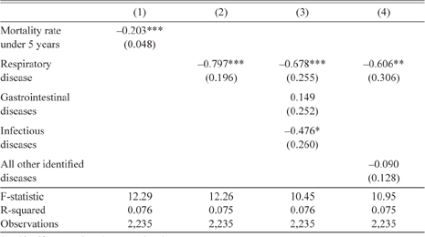
The association between height and district mortality rates is explored in Table 8, where individual and household variables are included but not reported. Clearly, as height and mortality rates are determined by local conditions these results are not causal. But it is useful to see which causes of mortality are most strongly correlated with height. The first column demonstrates the strong negative relationship between individual height and the overall death rate in the district of childhood residence. Clearly, any selection effect is overwhelmed by the scarring effect. That in turn suggests that specific causes of death will capture different attributes of the underlying disease environment. Column (2) includes only the death rate from “diseases of the respiratory system.” This gives an equally strong negative coefficient, which reflects the high correlation in the sample of 0.94 between mortality from respiratory diseases and total mortality.Footnote ³²

Table 8

Height and Child Mortality Rates

^* = Significant at the 10 percent level.

^** = Significant at the 5 percent level.

^*** = Significant at the 1 percent level.

Note: Robust standard errors, in parentheses, clustered at the county level. The dependent variable is height in inches. Mortality rates for children under five years in 1891–1900 are calculated by dividing the number of deaths (or the number by cause of death) by the average population in the age group over that period. Other controls, not reported, are age dummies for under 18, 18 and 19, number of siblings, a dummy for female head of household, a dummy for head of household in social classes 1 or 2, the number of rooms occupied (capped at 5), and ten regional dummies.

Source: Computed from data described in the text.

Column (3) adds variables for death rates from two more causes of death: gastrointestinal disease, which includes diarrhoea and dysentery as well as diseases of the digestive system; and infectious disease, which is the sum of deaths from measles, scarlet fever, diphtheria, and whooping cough. Gastrointestinal disease evidently adds little to the explanation of height, whereas infectious disease has a negative relationship with height that is significant at the 10 percent level. Even in the presence of these additional variables, respiratory disease retains significance. In the last column all identified causes of death other than respiratory disease are added together as one group. This takes an insignificant coefficient while death from respiratory disease remains significant.

The strong association of adult height with child mortality is consistent with the hypothesis that an individual’s disease environment restricted growth during childhood through a scarring effect. In light of the significance of mortality from respiratory disease in this process, we may suppose that respiratory infection was an important, if not the only, conduit for the observed relationship between atmospheric pollution and heights.Footnote ³³ Indeed, Beach and Hanlon (Reference Beach and Hanlon2018) report that coal intensity had a causal effect on mortality rates across registration districts in 1851–1860, and especially on deaths from respiratory diseases. Our results in Table 8 demonstrate a close association between adult height and child mortality, in the 1890s. Taken together these findings indicate that industrial emissions from coal combustion created a local disease environment that increased the risk of respiratory infection, which influenced both the probability of survival in childhood and the ongoing health of those who survived.