1 Introduction
In the Lagrangian framework, incompressible ideal fluids can be pictured as freely evolving space-filling assemblies of infinitely many classical ‘fluid particles’, whose internal energies are neglected, and whose collective dynamics is therefore conservative. It may hence come as no surprise that the Euler equations can be formally deduced from a Lagrangian least-action principle, whereby the action is the time integral of the total kinetic energy, while incompressibility appears as a non-holonomic constraint for the Lagrangian flow  $(\boldsymbol{a},t)\mapsto \boldsymbol{X}(\boldsymbol{a},t)$, which is assumed to be a smooth function of both time and the Lagrangian coordinates
 $\boldsymbol{a}$. For each time
 $t$, both the Lagrangian map
 $\boldsymbol{X}(\boldsymbol{\cdot },t)$ and the inverse ‘back-to-label’ map
 $\boldsymbol{X}^{-1}(\boldsymbol{\cdot },t)$ are deterministic objects, which are supposed to be well defined and sufficiently regular. In mathematical terms, this means that they belong to the class of ‘smooth diffeomorphisms’.
The deterministic Lagrangian least-action principle was made rigorous by Arnold (Reference Arnold1966) – see also Khesin & Arnold (Reference Khesin and Arnold2005), Arnold (Reference Arnold2013) and Farazmand & Serra (Reference Farazmand and Serra2018). It is at the root of the subsequent classical literature on the Hamiltonian formulation of ideal fluid dynamics, which has found widespread ramifications in the context of geophysical and plasma modelling – we refer the reader to the pedagogical reviews by Salmon (Reference Salmon1988), Shepherd (Reference Shepherd1990), Morrison (Reference Morrison1998) and references therein. To briefly emphasise the power of least-action principles, let us here just point out that Hamiltonian methods not only provide a practical guideline that can be used to control approximations in asymptotic models (Holm & Kupershmidt Reference Holm and Kupershmidt1983; Salmon Reference Salmon1983, Reference Salmon1985; Morrison Reference Morrison2005) and develop faithful numerical methods (Marsden & West Reference Marsden and West2001; Zeitlin Reference Zeitlin2004; Kraus, Tassi & Grasso Reference Kraus, Tassi and Grasso2016), but also lay the basis for systematic stability analyses (Holm et al. Reference Holm, Marsden, Ratiu and Weinstein1985; Abarbanel et al. Reference Abarbanel, Holm, Marsden and Ratiu1986) and formal statistical mechanics computations (Robert & Sommeria Reference Robert and Sommeria1991; Miller, Weichman & Cross Reference Miller, Weichman and Cross1992; Bouchet & Corvellec Reference Bouchet and Corvellec2010; Bouchet & Venaille Reference Bouchet and Venaille2012). In spite of its relevance when formally putting the viscosity to zero, Arnold’s Lagrangian formulation is not necessarily appropriate in the context of turbulence, that is to describe solutions to the Navier–Stokes equations in the limit of vanishing viscosity.
From a mathematical viewpoint, Arnold’s least-action principle yields spatially smooth solutions to the Euler equations. Yet, it is well known that the notion of solution to the Euler equations needs to be carefully weakened in order to craft velocity fields that reproduce hallmark turbulent features while remaining physical (see, e.g. Duchon & Robert (Reference Duchon and Robert2000) and Eyink (Reference Eyink2002)). To that end, the notion of distributional solutions with prescribed Hölder spatial regularity (also known as ‘rough’ solutions) has been particularly scrutinised in relation to a conjecture made by Onsager (Reference Onsager1949) – see also Eyink & Sreenivasan (Reference Eyink and Sreenivasan2006). It has been recently established (Buckmaster Reference Buckmaster2015; Buckmaster, Lellis & Székelyhidi Reference Buckmaster, Lellis and Székelyhidi2016; Isett Reference Isett2018) that dissipative rough solutions to the three-dimensional Euler equations do exist with a spatial Hölder exponent slightly below  $1/3$. This indicates that an inviscid dynamics could indeed be relevant to reproduce experimental measurements, including the persistence of a finite dissipation in the limit of infinite Reynolds number (the so-called ‘dissipative anomaly’, see Sreenivasan Reference Sreenivasan1984), the
 $4/5$ law (see, e.g. Antonia & Burattini (Reference Antonia and Burattini2006)) and possibly deviations to the Kolmogorov 1941 scaling (see, e.g. Saw et al. (Reference Saw, Debue, Kuzzay, Daviaud and Dubrulle2018)). It cannot be ruled out that constructing physical turbulent solutions to the Euler equations requires considering even weaker notions of solutions, examples of which include the measure-valued solutions of DiPerna & Majda (Reference DiPerna and Majda1987) – see also Brenier, De Lellis & Székelyhidi (Reference Brenier, De Lellis and Székelyhidi2011) – where the local velocity is not uniquely defined but rather prescribed by a local probability distribution.
At a physical level, a crucial consequence of the velocity being probabilistic is that fluid-element trajectories become themselves probabilistic: the deterministic concept of Lagrangian map is no longer appropriate to describe the dynamics. A similar consequence is conjectured to also hold true for the rough velocity fields imagined by Onsager: in such fields, initially coincident fluid particles are likely to separate in finite time, hereby becoming ‘spontaneously stochastic’ – see, e.g. Bernard (Reference Bernard2000), Falkovich, Gawȩdzki & Vergassola (Reference Falkovich, Gawȩdzki and Vergassola2001) and Gawȩdzki (Reference Gawȩdzki and Vassilicos2001). For such scenarios, generalised Lagrangian least-action principles, such as the one formulated by Brenier (Reference Brenier1989), could prove of particular relevance, and this is the long-term fundamental motivation for the present study.
Brenier’s formulation is essentially a probabilistic generalisation of Arnold’s principle. Roughly said, it consists in minimising a suitably defined average kinetic energy among a very wide class of stochastic processes – the so-called ‘generalised Lagrangian flows’ – rather than among the sole deterministic class of smooth diffeomorphisms. From a mathematical perspective, this generalisation guarantees the existence of minimisers under rather weak assumptions. The minimising generalised flow is no longer a time-parametrised collection of maps but rather defined as a probability distribution on the space of Lagrangian paths. The solution is obtained by prescribing boundary conditions in time, which amounts to specifying the Lagrangian transition probabilities from the initial to the final time. Let us note that this formulation of the problem does not rule out deterministic Lagrangian motion. In fact, it was shown by Brenier (Reference Brenier1989) that Arnold’s solutions are indeed retrieved by the generalised variational principle. In that case, the minimising generalised flow ‘concentrates’ around the deterministic solution and is formally described by a Dirac measure, meaning that random trajectories that are not arbitrarily close from the deterministic ones are unlikely to occur.
In concept, Brenier’s generalised flows are very general: they encompass the smooth solutions to the Euler equations produced by Arnold’s principle on the one hand, and on the other hand they turn out to provide a framework for explicit constructions of dissipative Euler solutions, with possible relevance to turbulence (Shnirelman Reference Shnirelman2000). Brenier’s least-action principle can be seen as a mathematical tool, which produces generalised flows that formally connect to the Euler equations (Brenier Reference Brenier1989, Reference Brenier1999, Reference Brenier2008).
In practice, Brenier’s principle is formulated as a two-end boundary-value problem rather than an initial-value one (later ‘Cauchy problem’). While the latter is the most usual formulation of fluid dynamics, boundary-value optimisation problems have found renewed interest among fluid dynamicists in the recent years. They naturally appear in a wide variety of applications, such as the prediction of extreme events and instanton theory (Laurie & Bouchet Reference Laurie and Bouchet2015; Dematteis, Grafke, Onorato & Vanden-Eijnden Reference Dematteis, Grafke, Onorato and Vanden-Eijnden2019), nonlinear control of fluid flows (Protas Reference Protas2008; Lecoanet & Kerswell Reference Lecoanet and Kerswell2018), closure theories (Protas, Noack & Östh Reference Protas, Noack and Östh2015; Thalabard & Turkington Reference Thalabard and Turkington2017) or data reconstruction from in situ measurements (Tu et al. Reference Tu, Griffin, Hart, Rowley, Cattafesta and Ukeiley2013; Van Nguyen, Laval & Chainais Reference Van Nguyen, Laval and Chainais2015). In that particular context, invoking Brenier’s principle to reconstruct Lagrangian dynamics is an obvious long-term perspective. Our intention here is to achieve a first step towards that end. We aim to assess the potential skills of the generalised least-action principle at coarse graining the Lagrangian motion of fluid particles, and reconstructing therefrom the Eulerian space–time dynamics of the associated velocity fields.
The intrinsic statistical features of the minimising flows depend on the input data: in Brenier’s formulation it is specified in terms of a two-end coupling, namely in terms of Lagrangian transition probabilities between initial and final times. If the input data are generated from Euler dynamics, one should rightfully wish that solving the generalised least-action principle yields back the full solution. This is indeed the case for short times, as proven by Brenier (Reference Brenier1989). Yet, having the mind set on data reconstruction, one would rather consider a physical scenario, where the input data would be generated by viscous dynamics (Navier–Stokes) and would necessarily be coarse grained in space. In those cases, one could still solve for the minimising generalised flows, but it is then unclear how relevant or even how physical those would be.
The present work clarifies this issue by narrowing the investigation into two distinct questions. The first question is fundamental: When the generalised minimisers cease to coincide with classical solutions to become truly non-deterministic, do their statistical features represent a transition towards a turbulent state? The second one is practical: can the generalised minimisers be used to construct a relevant coarse-grained space–time dynamics from non-trivial input data? Our answers to those questions turn out to be negative and positive respectively. Our argumentation relies on the numerical analysis of both the Eulerian and the Lagrangian features of selected two-dimensional generalised flows, that we generate by solving Brenier’s principle using input data of increasing complexity, ranging from solid rotation and cellular flows to freely decaying two-dimensional turbulence.
In order to compute Brenier’s solutions, we introduce a statistical-mechanics interpretation of the concept of generalised flows, whereby the latter become akin to statistical ensembles of suitably defined ‘permutation flows’. We then employ Monte Carlo techniques to numerically solve the generalised least-action principle, and estimate both the Eulerian and Lagrangian statistics of the generalised solution. In all the cases considered, the Lagrangian trajectories are in principle univocally defined at a microscopic level, and not spontaneously stochastic. While spatial coarse graining still calls for a probabilistic description of trajectories, we may a priori expect the minimising flows to be only mildly non-degenerate, at least if the Lagrangian trajectories are non-chaotic. Our analysis highlights a major caveat of the generalised variational principle, that produces non-physical dynamics when solved over long time intervals, e.g. longer than a well-defined hydrodynamic turnover time. We argue that this limitation is not specifically inherent to Brenier’s formulation, but rather to the variational framework being formulated as a two-end boundary-value problem: when solved over the same time lags, Arnold’s least-action principle also produces incorrect Euler solutions. When appropriately used over sufficiently short times, the generalised least-action principle is shown to be relevant, for all the examples considered. Besides, our third example shows that it also succeeds at reproducing irreversible Eulerian behaviours, such as the enstrophy and energy decays of 2-D decaying turbulence. This suggests that if carefully used, generalised variational formulations could provide new tools to coarse grain genuine multi-scale hydrodynamics.
The paper is organised as follows. In § 2 we formulate Arnold’s and Brenier’s least-action principles in a fluid-mechanical language. In § 3 we provide a discrete version of generalised flows that allows for numerical constructions based on Monte Carlo techniques. In § 4 we use this method with, as input data, a coarse-grained Lagrangian map associated with Beltrami (cellular) flows. By investigating the time variations of kinetic energy, the scaling properties of the velocity field and Lagrangian trajectories, we argue that generalised flows display non-physical features when the time lag between the initial and final times is too large. We then use such considerations to investigate the case of two-dimensional decaying turbulence in § 5. We observe that the generalised least-action principle allows us to reconstruct the coarse-grained velocity when the time lag is chosen of the order of or smaller than the large-eddy turnover time. Finally, we draw concluding remarks in § 6.
2 Lagrangian variational formulations of inviscid fluid dynamics
2.1 Arnold’s least-action principle
In order to set the framework for Brenier’s formulation, let us first formally restate Arnold’s variational formulation of ideal fluid dynamics. Beyond the virtue of setting up some notations, we will then already be in a position to comment on the existence of a critical time lag  $t_{\star }$, over which Arnold’s least-action principle becomes a weaker principle of stationary action: this unwanted feature will have a counterpart in Brenier’s formulation. To focus on general physical ideas, our exposition is intentionally phenomenological, and we refer the mathematically inclined reader to the book of Khesin & Arnold (Reference Khesin and Arnold2005) and the review of Ebin & Marsden (Reference Ebin and Marsden1970).
Arnold’s formulation is rooted on the deterministic Lagrangian viewpoint. The fluid is then nothing but the collection of individual fluid particles, which are labelled by some Lagrangian set of coordinates  $\boldsymbol{a}$, and whose trajectories determine its dynamics. The formalisation uses the concept of Lagrangian flow map
 $(\boldsymbol{a},t)\mapsto \boldsymbol{X}(\boldsymbol{a},t)$, which associates with each fluid particle its position at time
 $t$ within the physical domain
 ${\mathcal{D}}$. The projections
 $\boldsymbol{a}\mapsto \boldsymbol{X}(\boldsymbol{a},t)$ define the Lagrangian maps at time
 $t$, and the projections
 $t\mapsto \boldsymbol{X}(\boldsymbol{a},t)$ define the trajectories of particles with Lagrangian label
 $\boldsymbol{a}$. The Lagrangian flows are assumed to be smooth functions of both time and the Lagrangian coordinates. It is convenient to identify Lagrangian labels with the initial positions of fluid elements, so that
 $\boldsymbol{X}(\boldsymbol{a},0)=\boldsymbol{a}$. Hence, in the sequel, the initial map will always be taken as identity.
Lagrangian flows describe incompressible fluids when they preserve volumes, that is when the Jacobian determinant of the Lagrangian map satisfies  $|\unicode[STIX]{x2202}\boldsymbol{X}/\unicode[STIX]{x2202}\boldsymbol{a}|\equiv 1$. The Eulerian velocity field is then obtained from the particle velocities through
 $\boldsymbol{v}(\boldsymbol{X}(\boldsymbol{a},t),t)=\unicode[STIX]{x2202}_{t}\boldsymbol{X}(\boldsymbol{a},t)$. The total fluid kinetic energy therefore reads
 $$\begin{eqnarray}\displaystyle {\mathcal{E}}(t):=\int _{{\mathcal{D}}}\,\text{d}\boldsymbol{a}\,\frac{1}{2}\Vert \unicode[STIX]{x2202}_{t}\boldsymbol{X}(\boldsymbol{a},t)\Vert ^{2}. & & \displaystyle\end{eqnarray}$$
Arnold’s variational principle can now be stated as
 $$\begin{eqnarray}\displaystyle \left.\begin{array}{@{}l@{}}\displaystyle {\mathcal{A}}_{0,t_{f}}[\boldsymbol{X}(\boldsymbol{\cdot })]:=\int _{0}^{t_{f}}\,\text{d}t\,{\mathcal{E}}(t)\longrightarrow \text{inf}\quad \text{subject to}\\[5.0pt] \boldsymbol{X}(\boldsymbol{\cdot },0)=\boldsymbol{I},\quad \boldsymbol{X}(\boldsymbol{\cdot },t_{f})=\boldsymbol{X}_{f}(\boldsymbol{\cdot }),\text{ and }\left|{\displaystyle \frac{\unicode[STIX]{x2202}\boldsymbol{X}}{\unicode[STIX]{x2202}\boldsymbol{a}}}\right|\equiv 1.\end{array}\right\} & & \displaystyle\end{eqnarray}$$
The action functional  ${\mathcal{A}}_{0,t_{f}}$ appears as a natural counterpart to the actions used in textbooks for the formulation of classical finite-dimensional mechanics (see, e.g. José & Saletan (Reference José and Saletan2000)). It is obvious, but worth emphasising, that the formulation (2.2) defines a boundary-value optimisation problem, as both ‘endpoint’ maps
 $\boldsymbol{X}(\boldsymbol{\cdot },0)=\boldsymbol{I}$ and
 $\boldsymbol{X}_{f}(\boldsymbol{\cdot })$ at final time
 $t_{f}$ are prescribed. A formal way of solving (2.2) is to use a Lagrange multiplier
 $P(\boldsymbol{a},t)$ to enforce the incompressibility constraint, and compute the functional derivatives with respect to the flow
 $\boldsymbol{X}$ of the augmented action
 $A_{0,t_{f}}+\int _{0}^{t_{f}}\,\text{d}t\int _{{\mathcal{D}}}\,\text{d}\boldsymbol{a}\,P(\boldsymbol{a},t)\,(|\unicode[STIX]{x2202}\boldsymbol{X}/\unicode[STIX]{x2202}\boldsymbol{a}|-1)$. The optimal solutions necessarily solve the Euler–Lagrange equations. Requiring the action to be stationary (
 $\unicode[STIX]{x1D6FF}{\mathcal{A}}_{0,t_{f}}=0$), a string of formal calculations leads to
 $$\begin{eqnarray}\displaystyle \unicode[STIX]{x2202}_{tt}\boldsymbol{X}(\boldsymbol{a},t)=-[\unicode[STIX]{x2202}\boldsymbol{X}/\unicode[STIX]{x2202}\boldsymbol{a}]^{-1}\unicode[STIX]{x1D735}_{\boldsymbol{a}}P,\quad \text{with }|\unicode[STIX]{x2202}\boldsymbol{X}/\unicode[STIX]{x2202}\boldsymbol{a}|\equiv 1, & & \displaystyle\end{eqnarray}$$
which is exactly the Lagrangian formulation of the inviscid dynamics of an incompressible fluid. Note that (2.3) is second order in time, which means that we need two boundary conditions provided by the initial and final maps in Arnold’s principle (2.2).
2.2 Boundary-value formulation and turnover time
The boundary-value formulation of Arnold’s principle (2.2) is not usual in fluid mechanics. One rather considers the initial-value problem, which involves the initial fluid velocity  $\unicode[STIX]{x2202}_{t}\boldsymbol{X}(\boldsymbol{a},0)=\boldsymbol{v}_{0}(\boldsymbol{a})$ in addition to the initial map. However, as we will now see, the connection between these two formulations is not univocal.
It is easily understood that for an infinitesimally short time lag  $t_{f}$, there is a one-to-one correspondence between the initial velocity field and a final map that is sufficiently close to identity:
 $\boldsymbol{X}_{f}\approx \boldsymbol{I}+t_{f}\,\boldsymbol{v}_{0}$. This mapping actually extends to longer time lags and a given solution to the initial-value problem can then be retrieved by solving (2.2) with the appropriate boundary conditions. This is however true only up to a finite value
 $t_{\star }$ of the time lag. In fact, the critical time
 $t_{\star }$ can be heuristically understood as a turnover time. The reason why one-to-one correspondence breaks down for
 $t_{f}>t_{\star }$ becomes apparent when one considers simple examples of vortical flows. Let us for instance consider a two-dimensional solid-rotating flow in a disk of radius
 $R$. In Eulerian coordinates the velocity field reads
 $$\begin{eqnarray}\displaystyle \boldsymbol{v}_{\unicode[STIX]{x1D6FA}}(\boldsymbol{x},t)=\unicode[STIX]{x1D734}\times \boldsymbol{x}\quad \text{with }\unicode[STIX]{x1D734}:=\unicode[STIX]{x1D6FA}\hat{\boldsymbol{z}}\text{ a prescribed (constant) vorticity}. & & \displaystyle\end{eqnarray}$$
This is a steady solution to the Euler equations. The corresponding Lagrangian flow is obtained as
 $$\begin{eqnarray}\displaystyle \boldsymbol{X}_{\unicode[STIX]{x1D6FA}}(\boldsymbol{a},t)=\boldsymbol{a}\,\cos \unicode[STIX]{x1D6FA}t+\hat{\boldsymbol{z}}\times \boldsymbol{a}\,\sin \unicode[STIX]{x1D6FA}t. & & \displaystyle\end{eqnarray}$$
We can now seek to apply the boundary-value formulation (2.2) to reconstruct the rotating dynamics between time  $0$ and a final prescribed time
 $t_{f}$. The final map is naturally prescribed as
 $\boldsymbol{X}(\boldsymbol{\cdot },t_{f})=\boldsymbol{X}_{\unicode[STIX]{x1D6FA}}(\boldsymbol{\cdot },t_{f})$. Observe that this endpoint condition determines the rotation modulo
 $2\unicode[STIX]{x03C0}$ only: In other words, writing
 $\unicode[STIX]{x1D703}_{f}\in ]-\unicode[STIX]{x03C0},\unicode[STIX]{x03C0}]$ the principal value of the final angle
 $\unicode[STIX]{x1D6FA}\,t_{f}$, all the solid rotations with pulsation
 $\unicode[STIX]{x1D6FA}_{k}^{\prime }:=(\unicode[STIX]{x1D703}_{f}+2k\unicode[STIX]{x03C0})/t_{f}$ with
 $k\in \mathbb{Z}$ share the same final map. For such rotations, one explicitly computes Arnold’s action as
 $$\begin{eqnarray}\displaystyle {\mathcal{A}}_{0,t_{f}}={\displaystyle \frac{\unicode[STIX]{x03C0}R^{4}}{6}}\unicode[STIX]{x1D6FA}_{k}^{^{\prime }2}t_{f}={\displaystyle \frac{\unicode[STIX]{x03C0}R^{4}}{6t_{f}}}\,(\unicode[STIX]{x1D703}_{f}+2k\unicode[STIX]{x03C0})^{2}. & & \displaystyle\end{eqnarray}$$
When  $\unicode[STIX]{x1D703}_{f}<\unicode[STIX]{x03C0}$, the action is obviously minimal for
 $k=0$. Arnold’s principle therefore selects the rotation with pulsation
 $\unicode[STIX]{x1D6FA}_{\star }:=\unicode[STIX]{x1D6FA}_{k=0}^{\prime }=\unicode[STIX]{x1D703}_{f}/t_{f}$, and this in turn implies that Arnold’s minimiser only coincides with the desired rotation at pulse
 $\unicode[STIX]{x1D6FA}$ when
 $t_{f}<t_{\star }=\unicode[STIX]{x03C0}/\unicode[STIX]{x1D6FA}$. For
 $t_{f}>t_{\star }$, the minimiser is a solid rotation with a smaller vorticity
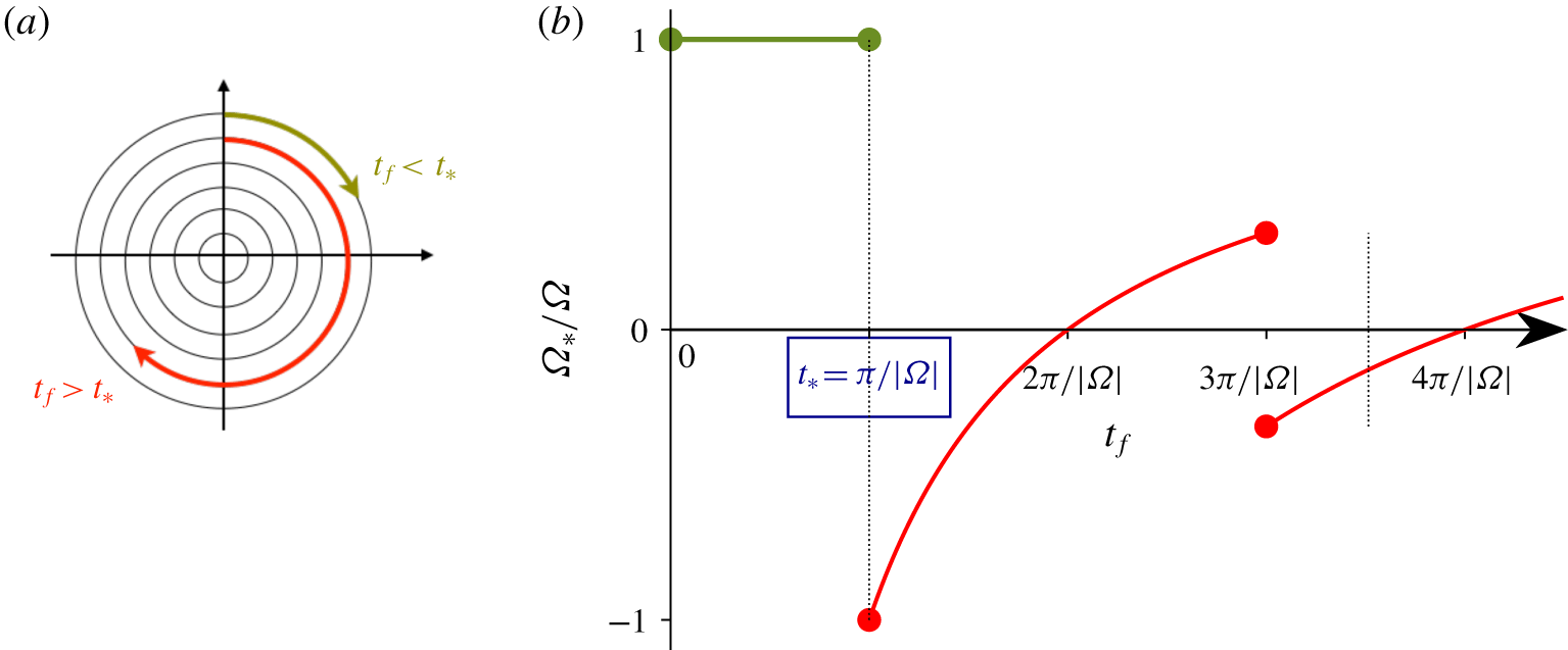
 $|\unicode[STIX]{x1D6FA}_{\star }|<\unicode[STIX]{x1D6FA}$ (see figure 1). Because it solves the Euler equations, the desired solid rotation prescribed by the initial-value problem still makes the action stationary but is not peculiar among the other critical points. It is also apparent in figure 1, and worth pointing out, that, except for the discrete set of final times
 ${t_{f}}_{k}=k\unicode[STIX]{x03C0}/\unicode[STIX]{x1D6FA},k\in \boldsymbol{Z}$, Arnold’s principle still selects a unique rotation. While it is not the desired rotation, Arnold’s principle still can be solved univocally. Such is not the case when
 $\unicode[STIX]{x1D703}_{f}=\unicode[STIX]{x03C0}$, which occurs at times
 ${t_{f}}_{k}=k\unicode[STIX]{x03C0}/\unicode[STIX]{x1D6FA},k\in \boldsymbol{Z}$, when the final map describes a system that has rotated by exactly half of a full turn. The minimal action is then achieved by both the clockwise (
 $k=0$) and anti-clockwise (
 $k=-1$) rotating flows: two minimisers exist and Arnold’s principle becomes unable to select a unique minimiser. Inducing from the solid-rotation example, it becomes intuitively clear that the presence of local rotation restricts the use of the boundary-value formulation in terms of Lagrangian maps. In that sense, the critical time
 $t_{f}$ can be tied to a notion of turnover time. When solved on time intervals larger than this critical time, Arnold’s principle (2.2) may fail to select the desired solution. In the solid-rotation case, the degeneracy relates to the final map being compatible with two different pulses at the same time, that generate equally energetic solutions. It will soon be apparent that this turnover time coincides with a critical time over which Brenier’s formulation generate genuinely probabilistic flows.
A solid-rotating flow with pulse  $\unicode[STIX]{x1D6FA}$ only solves the variational principle (2.2) up to final times
 $t_{f}<t_{\star }(\unicode[STIX]{x1D6FA})$ (in green), when the final map has rotated less than half a turn (a). For
 $t_{f}>t_{\star }$ (in red), the minimising vorticity
 $\unicode[STIX]{x1D6FA}_{\star }$ is lower and may even be of opposite sign. This can be seen in (b), which shows the action-minimising vorticity
 $\unicode[STIX]{x1D6FA}_{\star }$ as a function of the final time
 $t_{f}$.

2.3 Brenier’s least-action principle
As previously evoked, another restriction of Arnold’s description comes from its deterministic nature, even when  $t_{f}$ is small enough. In particular, the description of a fluid in terms of a flow map cannot appropriately reproduce the ‘rough’ solutions to the Euler equations that could be of relevance for inertial turbulence.
In Brenier’s generalisation of (2.2), the fluid is no longer defined in terms of a Lagrangian flow map  $\boldsymbol{X}(\boldsymbol{a},t)$, but rather in terms of a generalised flow: namely, a probability measure
 $\unicode[STIX]{x1D707}[\mathfrak{D}\unicode[STIX]{x1D738}]$ defined over Lagrangian trajectories
 $t\mapsto \unicode[STIX]{x1D738}(t)$. We only consider differentiable trajectories, so that one can define the time-integrated energy
 $$\begin{eqnarray}\displaystyle {\mathcal{S}}[\unicode[STIX]{x1D738}]={\displaystyle \frac{1}{2}}\int _{0}^{t_{f}}\,\text{d}t\,\Vert \unicode[STIX]{x2202}_{t}\unicode[STIX]{x1D738}(t)\Vert ^{2}. & & \displaystyle\end{eqnarray}$$
The Lagrangian random variable  ${\mathcal{S}}[\unicode[STIX]{x1D738}]$ is now the fundamental ‘energy functional’ quantity that generalises the action. Still, generalised flows also require generalised constraints. Essentially, we prescribe to a fixed distribution the two-time probability
 $\unicode[STIX]{x1D707}|_{0,t_{f}}$ of
 $t=0$ and
 $t=t_{f}$, which is obtained as a marginal of
 $\unicode[STIX]{x1D707}$. As for the incompressibility constraint, it translates into imposing that the one-time distributions
 $\unicode[STIX]{x1D707}|_{t}$, given again by
 $\unicode[STIX]{x1D707}$, stay uniform as a function of time. Brenier’s least-action principle can now be formally stated,
 $$\begin{eqnarray}\displaystyle \left.\begin{array}{@{}c@{}}{\mathcal{B}}_{0,t_{f}}[\unicode[STIX]{x1D707}]:=\displaystyle \int \unicode[STIX]{x1D707}[\mathfrak{D}\unicode[STIX]{x1D738}]\,{\mathcal{S}}[\unicode[STIX]{x1D738}]\longrightarrow \text{inf}\quad \text{subject to}\\ \unicode[STIX]{x1D707}|_{0,t_{f}}=\unicode[STIX]{x1D707}_{0,f}\quad \text{and}\quad \unicode[STIX]{x1D707}|_{t}\text{ uniform}.\end{array}\right\} & & \displaystyle\end{eqnarray}$$
The probabilistic constraints are on marginals of the distribution  $\unicode[STIX]{x1D707}$, whence the relationship with multi-marginal optimal transport. Because there is a probabilistic coupling
 $\unicode[STIX]{x1D707}_{0,f}$ between the initial and final positions, the formulation (2.8) is again a boundary-value problem.
The generalised least-action principle (2.8) was conceptualised by Brenier (Reference Brenier1989) – see also Brenier (Reference Brenier2008) – with some established mathematical properties, including:
(i) Generalised solutions to (2.8) exist for very general endpoint couplings
 $\unicode[STIX]{x1D707}_{0,f}$.
(ii) The generalised variational principle encompasses classical (regular) solutions, provided that the final time
$t_{f}$ is small enough. This requires choosing a deterministic endpoint coupling, which is prescribed by the map associated with a solution to the Euler equations, i.e. $\unicode[STIX]{x1D707}_{0,f}(\text{d}\boldsymbol{a},\text{d}\boldsymbol{x})=|{\mathcal{D}}|^{-1}\unicode[STIX]{x1D6FF}(\boldsymbol{X}_{f}(\boldsymbol{a})-\boldsymbol{x})\,\text{d}\boldsymbol{a}\,\text{d}\boldsymbol{x}$. The solution to (2.8) is then highly degenerate, concentrated on the deterministic Lagrangian flow. This requires $t_{f}<t_{\star }$ with (2.9)with$$\begin{eqnarray}\displaystyle t_{\star }={\displaystyle \frac{\unicode[STIX]{x03C0}}{\sup _{\boldsymbol{x},t}\Vert \text{Hessian}(p)\Vert ^{1/2}}}, & & \displaystyle\end{eqnarray}$$$p$ denoting the pressure field appearing in the underlying Euler equations.(iii) For
$t_{f}>t_{\star }$, generalised flows can become non-deterministic: the flow is no more described by the Lagrangian map, but rather by transition probabilities. A generalised ‘fluid particle’ tagged by its initial position then splits mass and have a multiplicity of subsequent positions at time $t$ prescribed by the two-time marginals $\unicode[STIX]{x1D707}|_{0,t}$.





Point (ii) above shows that (2.8) is indeed a generalisation of (2.2). Yet, the short-time restriction of Arnold’s boundary-value formulation remains: seemingly, considering  $t_{f}>t_{\star }$ might not be of physical relevance. Note in passing that for a solid rotation the pressure field is
 $p(x,y)=(\unicode[STIX]{x1D6FA}/2)^{2}(x^{2}+y^{2})$, yielding in that case
 $t_{\star }=\unicode[STIX]{x03C0}/|\unicode[STIX]{x1D6FA}|$ as obtained in § 2.2. In fact, the ‘generalised’ aspect of (2.8) relates to the type of Euler solutions that it can construct. Those can in principle include weak solutions to the Euler equations, be them distributional or even measure valued (Brenier Reference Brenier1999). In those cases, the generalised flow is always non-deterministic, even at short
 $t_{f}$.
In addition to those conceptual features, Brenier’s formulation has also a practical outcome: while (2.2) is a highly nonlinear problem which is cumbersome to use in practice, (2.8) is a linear optimisation problem, that is, a problem in which both the objective function and the constraints depend linearly on the arguments to be minimised upon. Various numerical methods are known, that can efficiently handle either low-dimensional or high-dimensional linear searches (Nocedal & Wright Reference Nocedal and Wright2006; Mérigot & Mirebeau Reference Mérigot and Mirebeau2016; Benamou, Carlier & Nenna Reference Benamou, Carlier and Nenna2019; Gallouët & Mérigot Reference Gallouët and Mérigot2018).
The relevance of generalised flows when used in combination with turbulent inputs can therefore be tested, and this remarkable feature provides the guideline for the remainder of the paper.
3 Statistical physics of generalised flows
The generalised variational principle (2.8) connects inviscid fluid mechanics with multimarginal optimal transport. Its numerical integration can thus benefit from the efficient algorithms that have been developed to solve such optimisation problems. In recent years, (2.8) has even been used as a test ground in the development of such methods – see for instance Brenier (Reference Brenier2008), Benamou et al. (Reference Benamou, Carlier, Cuturi, Nenna and Peyré2015), Mérigot & Mirebeau (Reference Mérigot and Mirebeau2016), Nenna (Reference Nenna2016), Benamou et al. (Reference Benamou, Carlier and Nenna2019) and Gallouët & Mérigot (Reference Gallouët and Mérigot2018). Here we follow a different strategy. We rather rely on a Monte Carlo algorithm, as the latter proves sufficient for our present scope. It stems from an intuitive statistical-mechanics interpretation of (2.8).
3.1 Coarse graining and permutation flows
It is illuminating to reformulate (2.8) in a discrete setting, both in space and in time. Specifically, we discretise time into  $N_{t}$ steps
 $t_{0}=0,t_{1},\ldots ,t_{N_{t}}=t_{f}$, and partition the
 $d$-dimensional physical domain
 ${\mathcal{D}}$ into
 $N_{x}^{d}$ ‘boxes’ of equal volume, and labelled by the
 $d$-dimensional indices
 $\boldsymbol{i}=(i_{1},\ldots ,i_{d})\in [1,N_{x}]^{d}$. In this ‘coarse-grained’ description, Lagrangian trajectories become sequences of indices
 $\{{\boldsymbol{i}_{n}\}}_{n=0..N_{t}}$, and generalised flows become finite-dimensional tensors, represented by the non-negative
 $(N_{x}^{d})^{N_{t}}$ entries
 $\unicode[STIX]{x1D707}\{\boldsymbol{i}_{n}\}:=\unicode[STIX]{x1D707}(\boldsymbol{i}_{0},\boldsymbol{i}_{1},\ldots ,\boldsymbol{i}_{N_{t}})$ normalised to
 $1$. One can now think of an incompressible generalised flow in two equivalent ways:
(i) In the ‘linear-programming viewpoint’, it is a measure with uniform single-time marginals, that is
(3.1)In this discrete setting, the optimisation problem (2.8) consists in minimising a suitably discretised average linear energy functional$$\begin{eqnarray}\displaystyle \unicode[STIX]{x1D707}_{k}(\boldsymbol{i}_{k}):=\mathop{\sum }_{\boldsymbol{i}_{0}\ldots \boldsymbol{i}_{k-1},\boldsymbol{i}_{k+1}\ldots \boldsymbol{i}_{N_{t}}}\unicode[STIX]{x1D707}\{\boldsymbol{i}_{n}\}=1/N_{x}^{d},\quad \text{for all }k=0\ldots N_{t}. & & \displaystyle\end{eqnarray}$$$\unicode[STIX]{x1D707}\mapsto \sum _{\boldsymbol{i}_{n}}\unicode[STIX]{x1D707}\{\boldsymbol{i}_{n}\}{\mathcal{E}}_{d}\{\boldsymbol{i}_{n}\}$, over the non-negative tensors $\unicode[STIX]{x1D707}$ satisfying the single-time marginal constraints (3.1), and two-time boundary coupling prescribed in the form of a doubly stochastic matrix, assigning a transition probability from box $\boldsymbol{i}$ to box $\boldsymbol{j}$ between initial and final time. In this formulation, it is apparent that the fluid parcel in box $\boldsymbol{i}$ at initial time is allowed to split mass. This is natural provided that one interprets the generalised flow as a spatial coarse graining of the Lagrangian trajectories. Taking the joint limit $N_{t}\rightarrow \infty ,N_{x}\rightarrow \infty$ one formally retrieves the continuous formulation (2.8). We refer the interested reader to the pedagogic review chapters of Nenna (Reference Nenna2016) for precise mathematical statements describing the convergence of discrete solutions towards time-continuous minimising flows.(ii) In the ‘statistical mechanics viewpoint’, it is a measure prescribed by a certain ensemble average over ‘permutation flows’
$\unicode[STIX]{x1D748}$ (Brenier Reference Brenier2008), that is (3.2)$$\begin{eqnarray}\displaystyle \unicode[STIX]{x1D707}\{\boldsymbol{i}_{n}\}\equiv {\displaystyle \frac{1}{N_{x}^{d}}}\mathop{\left\langle \mathop{\prod }_{k=1}^{N_{t}}\unicode[STIX]{x1D6FF}_{\boldsymbol{i}_{k}\unicode[STIX]{x1D748}_{k}(\boldsymbol{i}_{0})}\right\rangle }\nolimits_{\unicode[STIX]{x1D748}}. & & \displaystyle\end{eqnarray}$$







In the previous formula, each  $\unicode[STIX]{x1D748}_{n}$ is a permutation over the
 $N_{x}^{d}$ boxes between step
 $0$ and step
 $n$. Taking
 $\unicode[STIX]{x1D748}_{0}=\boldsymbol{I}$, the sequence
 $\{\unicode[STIX]{x1D748}_{n}(\boldsymbol{i})\}_{n=0..N_{t}}$ then represents the coarse graining of a Lagrangian trajectory starting from box
 $\boldsymbol{i}$, and the sequence
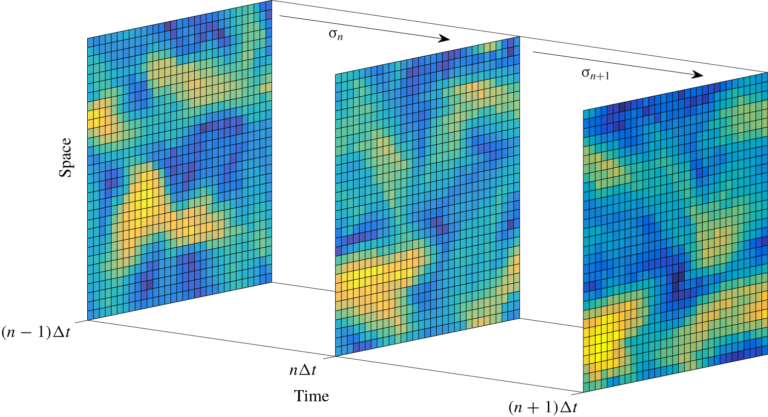
 $\unicode[STIX]{x1D748}=\{{\unicode[STIX]{x1D748}_{n}\}}_{n=0..N_{t}}$ is termed the ‘permutation flow’ (see illustration in figure 2). With this second interpretation at hand, we can now reformulate (2.8) in terms of an optimal statistical ensemble of permutation flows.
Illustration of a realisation of two-dimensional permutation flow. Colours code the initial positions.

3.2 Generalised solutions as statistical ensembles of permutation flows
Each realisation of a permutation flow yields the discrete action
 $$\begin{eqnarray}\displaystyle {\mathcal{A}}_{0,N_{t}}[\unicode[STIX]{x1D748}]=\mathop{\sum }_{n=1}^{N_{t}}{\mathcal{E}}_{n}\quad \text{with}~{\mathcal{E}}_{n}=\mathop{\sum }_{\boldsymbol{i}}\Vert \unicode[STIX]{x1D748}_{n}(\boldsymbol{i})-\unicode[STIX]{x1D748}_{n-1}(\boldsymbol{i})\Vert ^{2}, & & \displaystyle\end{eqnarray}$$
where  $\Vert \boldsymbol{i}-\boldsymbol{j}\Vert$ denotes here the discrete distance in
 $\mathbb{Z}^{d}$ between the centres of boxes
 $\boldsymbol{i}$ and
 $\boldsymbol{j}$. We now formulate the discrete counterpart to (2.8) as an optimisation over discrete measures
 $p[\unicode[STIX]{x1D748}]$ defining statistical ensembles of permutation flows
 $$\begin{eqnarray}\displaystyle {\mathcal{B}}_{0,N_{t}}[p]:=\mathop{\sum }_{\unicode[STIX]{x1D748}}{\mathcal{A}}_{0,N_{t}}[\unicode[STIX]{x1D748}]\,p[\unicode[STIX]{x1D748}]\longrightarrow \text{inf}\quad \text{subject to}~\mathop{\sum }_{\unicode[STIX]{x1D748}}\unicode[STIX]{x1D748}_{N_{t}}\,p[\unicode[STIX]{x1D748}]=\unicode[STIX]{x1D707}_{0\rightarrow t_{f}},\quad & & \displaystyle\end{eqnarray}$$
where  $\unicode[STIX]{x1D707}_{0\rightarrow t_{f}}$ is the transition probability from initial to final time. Using the standard matrix representation of permutations,
 $\unicode[STIX]{x1D707}_{0\rightarrow t_{f}}$ is an
 $N_{x}^{d}\times N_{x}^{d}$ doubly stochastic matrix. The discrete formulation (3.4) reveals that Brenier’s formulation resembles an averaged Arnold’s principle, whereby averages are taken with respect to measure-preserving applications, a set which includes but is not restricted to smooth volume-preserving maps.
The optimal statistical measure that solves (3.4) is discrete, but its dimensionality is huge (explicitly:  $(N_{x}^{d})!^{N_{t}}$)! Monte Carlo algorithms are thus particularly suited to obtaining numerical estimates of averages with respect to the optimal flow. Specifically, the formulation (3.4) can be formally understood as the zero-temperature/infinite-
 $\unicode[STIX]{x1D6FD}$ limit of the Gibbs canonical measure
 $$\begin{eqnarray}\displaystyle p_{\unicode[STIX]{x1D6FD}}[\unicode[STIX]{x1D748}]=\frac{1}{Z(\unicode[STIX]{x1D6FD})}\text{e}^{-\unicode[STIX]{x1D6FD}\,{\mathcal{A}}_{0,N_{t}}[\unicode[STIX]{x1D748}]}\quad \text{with associated averages }\langle \cdot \rangle _{\unicode[STIX]{x1D6FD}}. & & \displaystyle\end{eqnarray}$$
For finite temperatures, Monte Carlo averages are then easily sampled using a local Metropolis algorithm (see, e.g. Binder (Reference Binder1986)) on a  $(d+1)$-dimensional lattice, with the extra dimension representing the time axis. Algorithm 1 provides the pseudo-code of a single Monte Carlo iteration in our two-dimensional setting. We note that the finite-temperature regularisation is probably a statistical-mechanics counterpart to the concept of entropic regularisation used by Nenna (Reference Nenna2016) to implement efficient iterative projection algorithms rooted in the ‘linear programming viewpoint’. As a side remark, one can also point out that a realisation of a permutation flow, as represented in figure 2 and defined by the energy functional (3.3), may as well be thought of as a configuration of a generalised Potts model with
 $N_{x}^{d}$ colours and anisotropic nearest-neighbour interactions (see e.g. Baxter (Reference Baxter2016)).

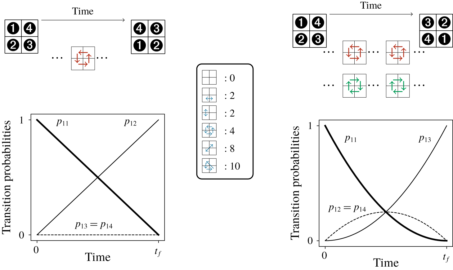
The solid-rotation example, this time interpreted as an ensemble of permutation flows on a coarse  $(2\times 2)$-box: nothing but a sliding puzzle. The middle inset provides the energy cost of the representative elementary permutations: permutation flows are discrete sequences of
 $N_{t}$ such elementary permutations, and the minimising discrete generalised flow is defined as the uniform probability measure over the set of permutation flows with minimal energy cost. Panels (a,b) represent the minimal permutation flows, when the final permutation is either a quarter of a full turn (a) or half of a full turn (b). The physical trajectory is uniquely defined in the first case as an anti-clockwise rotation. In the second case, the generalised flow is an average over both clockwise and anti-clockwise half-turn rotations. Panels (c,d) represent the time evolution of Lagrangian transition probabilities for the corresponding generalised flow, obtained in the limit
 $N_{t}\rightarrow \infty$ (see text for details).

3.3 Large-time limit of optimal permutation flows
One apparent virtue of (3.4) lies in its ability to produce unique generalised minimisers, when Arnold’s approach can fail to select one. From the perspective of discrete permutation flows, one can however hint that the uniqueness of such generalised minimisers (3.4) resembles a mathematical artefact rather than a new physical solution. Let us for instance revisit the solid-rotation example of § 2.2, in terms of a very coarse generalised flow involving a  $(2\times 2)$-spatial discretisation and
 $N_{t}$ time steps of length
 $\unicode[STIX]{x0394}t:=t_{f}/N_{t}$. In the solid-rotation example, and as was apparent in figure 1, we recall that Arnold’s principle only failed to select a solution when the final map represents half of a complete turn, in which case both clockwise and anti-clockwise rotations were equally energetic. Figure 3 illustrates how the permutation flow viewpoint accommodates this degeneracy. When the final state is say an anti-clockwise quarter of a full turn, the permutations flows with minimal costs are the sequences of permutations
 $\unicode[STIX]{x1D70E}_{1}\cdots \unicode[STIX]{x1D70E}_{N_{t}}$, where except for one non-trivial
 $\unicode[STIX]{x1D70E}_{t}:=\circlearrowright$ representing an anti-clockwise 4-cycle, every other one is the identity. The generalised minimiser is then obtained as the uniform average over those permutation flows, and the Lagrangian trajectories
 $\boldsymbol{X}(t,\boldsymbol{i})$ starting at prescribed
 $\boldsymbol{i}$ are then uniquely defined in physical space. Using elementary combinatorics, one can compute the transition probabilities
 $p_{\boldsymbol{i}\boldsymbol{j}}(t):=\unicode[STIX]{x1D707}(\boldsymbol{X}(t,\boldsymbol{i})=\boldsymbol{j})$ and obtain in the limit
 $N_{t}\rightarrow \infty$,
 $p_{13}=p_{14}=0$, together with
 $p_{11}=1-p_{14}=1-t/t_{f}$. Rightfully, the generalised solution predicts that no particle starting in the top-left box
 $\boldsymbol{i}_{0}=1$ transits diagonally or to its left before going down, and this generalised dynamics is represented in figure 3(a).
We can now consider the case when the final state is half of a full turn, and this situation is shown in figure 3(b). The permutations flows with minimal costs are now the sequences of permutations, containing exactly two non-trivial 4-cycle at arbitrary times  $(t_{1},t_{2})\in [|1,N_{t}|]^{2}$, that is
 $\unicode[STIX]{x1D70E}_{t_{1}}=\unicode[STIX]{x1D70E}_{t_{2}}:=\circlearrowright$ or
 $\unicode[STIX]{x1D70E}_{t_{1}}=\unicode[STIX]{x1D70E}_{t_{2}}:=\circlearrowleft$. The Lagrangian trajectories are then non-uniquely defined but the generalised solution is. In the limit
 $N_{t}\rightarrow \infty$, one for instance obtains the following transition probabilities:
 $p_{12}=p_{14}=(t/t_{f})(1-t/t_{f})$, and
 $p_{11}=(1-t/t_{f})^{2}$,
 $p_{13}=(t/t_{f})^{2}$. Particles contained in the top-left box have now equal probability to either clockwise or anti-clockwise transit towards the bottom-right corner.
It is apparent that the mass splitting is somewhat artificial: it solves the degeneracy of the deterministic problem by superimposing the possible trajectories and allowing the particles to feel both clockwise and anti-clockwise rotations at the same time. This toy argument suggests that there could be no physical meaning for the generalised variational formulation when Arnold’s principle breaks down. With that hint in mind, we can now study the physical properties of more intricate generalised flows, for which the vorticity field is no longer a mere constant of space and time, and the final map no longer necessarily degenerate.
4 Generalised flows and Beltrami dynamics
Beltrami flows are a class of strong Euler solutions of next-order complexity compared to solid rotations: while stationary, their vorticity is not constant in space. It is therefore instructive to study the statistical features of the generalised flows induced when using Beltrami Lagrangian maps as boundary conditions. Using our Monte Carlo algorithm, we find that the generalised flows indeed reproduce the intermediate Lagrangian dynamics of Beltrami flows for small times. For large final times, the Lagrangian flow breaks down. Even if this could have a promising ‘turbulent flavour’ and provide a possible framework to model intrinsic stochasticity, a deeper analysis of their statistical features reveals that such generalised flow are actually unphysical.
4.1 Generalised flows from Beltrami maps
We consider the one-cell Beltrami flow defined by the Eulerian velocity field on the domain  ${\mathcal{D}}=[0,1]^{2}$,
 $$\begin{eqnarray}\displaystyle \boldsymbol{v}(\boldsymbol{x},t)=(\cos \unicode[STIX]{x03C0}y\,\sin \unicode[STIX]{x03C0}x,-\cos \unicode[STIX]{x03C0}x\,\sin \unicode[STIX]{x03C0}y)^{\mathsf{T}}, & & \displaystyle\end{eqnarray}$$
from which we obtain explicitly  $t_{\star }=1$ using Brenier’s formula (2.9). Tracer particles are used to generate Beltrami permutation maps on a
 $64^{2}$ spatial grid at different prescribed final times. The generalised flows are then constructed with fixed time step
 $\unicode[STIX]{x0394}t=t_{\star }/8$. For instance, when
 $t_{f}=t_{\star }$, the discretisation has parameters
 $N_{x}=64$ and
 $N_{t}=8$ in the notations of § 3. To ensure that a statistical steady state is attained, averages are computed after routinely discarding the first
 $10^{6}$ Monte Carlo times (one Monte Carlo time is standardly defined as
 $N_{x}^{2}\times N_{t}$ iterations of the algorithm), and then using the data generated over the next
 $2.5\times 10^{5}$ ones. Our numerics clearly show that
 $t_{\star }=1$ marks a transition between a deterministic and a stochastic regime for the generalised flow.
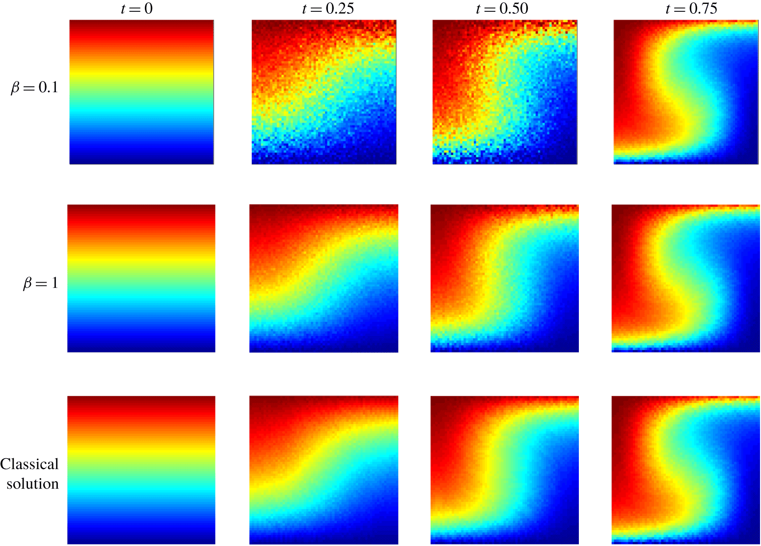
Reconstruction of the Beltrami dynamics as a function of time and  $\unicode[STIX]{x1D6FD}$ for
 $t_{f}=0.75<t_{\star }$. The colour code stands for the initial
 $y$ position of fluid particles.

4.2 The case $t_{f}<t_{\star }$: convergence toward Beltrami dynamics

When  $t_{f}<t_{\star }$, it is found that the Gibbs measures
 $\langle \cdot \rangle _{\unicode[STIX]{x1D6FD}}$ concentrate around the deterministic dynamics in the limit of zero temperature,
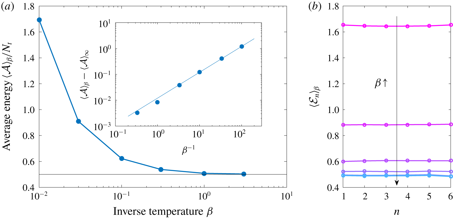
 $\unicode[STIX]{x1D6FD}\rightarrow \infty$. This can be seen in figure 4: For small enough temperatures, the average Lagrangian maps become essentially indistinguishable from those associated with the deterministic Beltrami flows, up to some small remaining thermal noise. This convergence towards the optimal ensemble is shown more clearly in figure 5: as
 $\unicode[STIX]{x1D6FD}$ increases, the average action converges towards the Beltrami action, which, as we know, solves (3.4) when
 $t_{f}<t_{\star }$. As shown in the inset, the convergence is algebraic
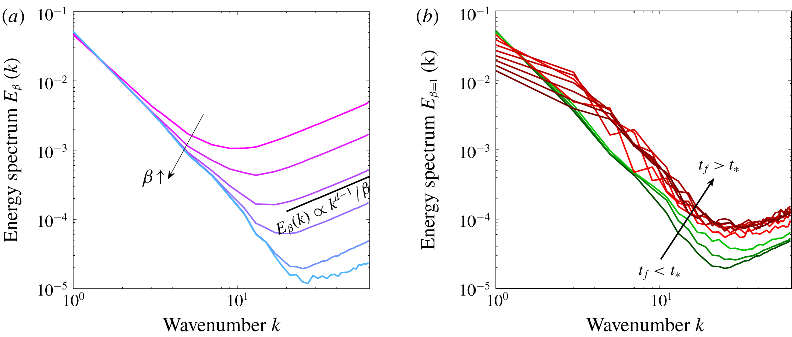
 $\propto \unicode[STIX]{x1D6FD}^{-1}$. Moreover, it is apparent from figure 5(b) that energy is conserved in time. This is a signature of the high regularity of such a classical solution to the Euler equations. This observed regularity is a consequence of the variational principle and was definitely not prescribed. This shows the effectiveness of Brenier’s variational principle in accommodating strong, classical, deterministic solutions, in spite of its probabilistic nature. Finally, let us note that the ‘finite-temperature effects’ are apparent on the spectra of the displacement and translate into small-scale thermalisation, namely equipartition of energy (see figure 6a). The range of thermalised scales naturally decreases with increasing
 $\unicode[STIX]{x1D6FD}$. Those features show the roundabout behaviour of our numerical procedure. They illustrate the established fact that for small enough
 $t_{f}<t_{\star }$ the generalised formulation (2.8) does indeed reproduce Arnold’s minimisers of (2.2) when those exist, as proven in Brenier (Reference Brenier1989).
Convergence of the action for the case  $t_{f}<t_{\star }$. Panel (a) shows convergence at zero temperature of the time-averaged kinetic energy – given by the action in (3.4) – towards the optimal Beltrami action. Panel (b) shows the time dependence of the generalised flow energy for inverse temperatures
 $\unicode[STIX]{x1D6FD}=0.01$,
 $0.03$,
 $0.1$,
 $0.3$,
 $1$ and
 $3$ (from top to bottom).

Kinetic energy spectra for (a)  $t_{f}<t_{\star }$ and various
 $\unicode[STIX]{x1D6FD}$ (same values as figure 5a) and (b) for
 $\unicode[STIX]{x1D6FD}=1$ fixed and various
 $t_{f}$ ranging from
 $0.75$ up to
 $2$ every
 $0.125$. The curves corresponding to
 $t_{f}<t_{\star }$ are shown in green, the others in red.

4.3 The case $t_{f}>t_{\star }$: non-physical behaviour of the generalised flow

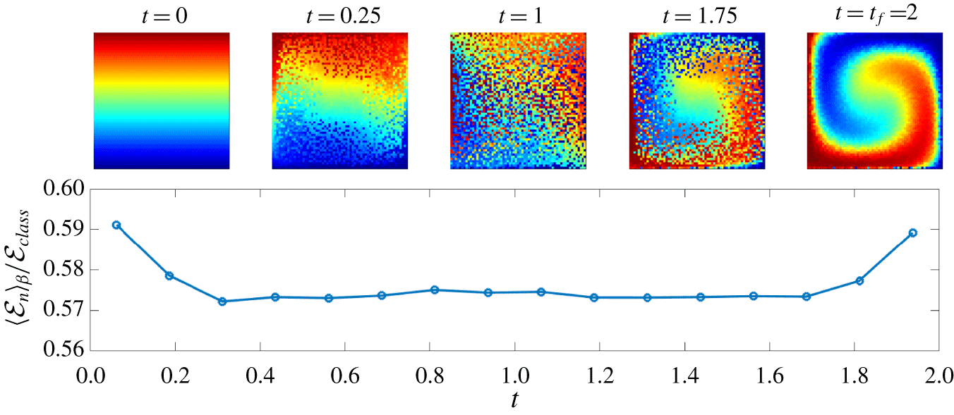
When  $t_{f}>t_{\star }$, the behaviour of the generalised flow becomes non-deterministic, and the time conservation of energy breaks down – see figure 7. This implies in particular that generalised flows cannot solve the Euler equations in a strong sense any longer. Yet, it is also apparent that the flow is not dissipative: the variations in the energy profile shown in (b) are symmetric and localised at the boundaries. Those behaviours are non-physical and likely consequences of both the time symmetry and the boundary-value formulation of the principle (2.8) itself. In the example chosen for figure 7, the breakdown of the Lagrangian flow is particularly spectacular for
 $t=t_{f}/2=1$. The nearly uniform colour pattern shows that initially distant pockets of fluid become arbitrarily close to each other at intermediate times before separating again. This is the signature of trajectory crossings. This picture may misleadingly suggest that generalised solutions essentially produce a thermalised dynamics, with fluid motion occurring at random. This is however not the case, as revealed by looking at the Eulerian spectra of the generalised displacement that are displayed in figure 6(b). While the small scales are indeed thermalised, the thermalisation is rather likely a spurious finite-temperature effect due to our numerical procedure, as its spread in
 $k$-space is not much wider than in the
 $t_{f}<t_{\star }$ case. The generalised flows obtained for
 $t_{f}>t_{\star }$ however display specific large-scale dynamics, which carry far less energy than the deterministic counterparts, whence their selections as optimal flows. We also note that, apart in the spurious thermalised range, the specific scalings displayed by the Beltrami generalised flows have no known counterparts in the phenomenology of two-dimensional turbulence.
(a) Typical permutation flow for the generalised solution with  $t_{f}=2t_{\star }$. We again show here, as a coloured background, the initial
 $y$ label as a function of time. (b) Time evolution of the kinetic energy. It is no longer conserved, and exhibits significant variations at the time boundaries.

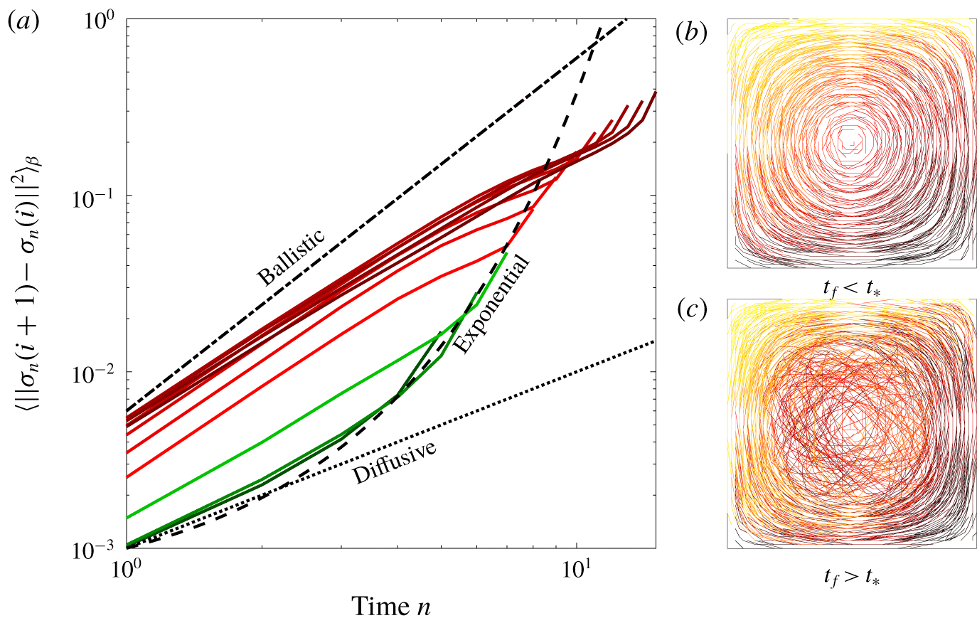
Perhaps this is even better seen from the Lagrangian measurements shown in figure 8. As can be seen in (a), the motions of fluid particles transit from a diffusive towards a faster ballistic regime when  $t_{f}$ is increased. The present breakdown of the Lagrangian flow is therefore not related to the phenomenon of explosive turbulent separation, nor to Richardson’s diffusion. The origin of a ballistic behaviour can actually be identified by looking at specific realisations of the generalised Beltrami trajectories. One indeed observes in figure 8(b,c) that for
 $t_{f}>t_{\star }$ that trajectories located at the centre of the domain ‘tunnel’ through the large-scale vortex to reach almost ballistically their final prescribed location. The statistics is then dominated by such displacements, which prove more efficient at transporting energy than classical rotating motions. Deviations to a purely ballistic regime come from the Lagrangian trajectories in a thin layer near the domain boundary, which remain ‘classical’: this is likely a consequence of the non-uniform distribution in Beltrami flows of vorticity, which is weaker at the boundary than at the centre of the domain.
(a) Average Lagrangian displacement for both  $t_{f}<t_{\star }$ (green)
 $t_{f}>t_{\star }$ (red). (b,c) Realisations of the Lagrangian trajectories, again for time lags
 $t_{f}$ below (b) and above (c) the critical time
 $t_{\star }$. The colour scale there codes the initial vertical positions of the trajectory.

4.4 Comments
The statistical analysis on generalised Beltrami flows confirms the intuition built from the  $(2\times 2)$ solid-rotation model considered in § 3.3: the transition from deterministic to non-deterministic generalised flows is not at any rate a transition to turbulence, however appealing this would have sounded. The generalised flows above
 $t_{\star }$ display a number of non-physical features, ranging from non-monotonic sharp variations of the energy at initial and final times, to ‘vortex-tunnelling’ ballistic motions of fluid trajectories. These highly undesirable specificities could possibly be avoided by further constraining the Lagrangian variational principle. For example, one can break the time-symmetric formulation by enforcing that energy be decreasing. On the one hand, this path could likely be a dead end as it is clear, already for Arnold’s regular geodesic, that the ‘
 $t_{\star }$ barrier’ is a defect of the boundary-value formulation, but not of the least-action principle. On the other hand, further constraining the Lagrangian trajectories may allow us to formulate Brenier’s principle as a non-trivial free-end optimisation problem (namely an initial-value problem in the language of partial differential equations), hereby wiping off artefacts due to the boundary-value formulation. At this point, our results therefore suggest that variational reconstructions of intermediate (turbulent) dynamics cannot rely solely on (2.8). It also requires an amount of data that ensures sufficiently close time-boundary conditions. Only at this price can one obtain a non-spurious ‘
 $t<t_{\star }$’ behaviour. With that in mind, we next apply least-action principles to turbulent data.
5 Generalised flows and decaying two-dimensional turbulence
The next step of our approach is to consider even more realistic cases, where vorticity varies not only in space but also in time. This is natural when one has in mind turbulent dynamics. Yet, the least-action principle that we have discussed is restricted to velocity fields solving the Euler equations. The classical solutions that were considered so far are of limited relevance to turbulent flows. In particular, they are too regular to occur as non-trivial limits of solutions to the Navier–Stokes equations when the viscosity  $\unicode[STIX]{x1D708}\rightarrow 0$. In that context, it is believed that weak (irregular) solutions to the Euler equations are more suitable candidates. Generalised least-action principle would be particularly useful if they could be used to tackle such non-smooth velocity fields. We naturally have in mind the possibility of addressing three-dimensional flows, but we here restrict ourselves to the problem of the two-dimensional direct enstrophy cascade.
It has been known since Batchelor (Reference Batchelor1969) that two-dimensional turbulence does not dissipate kinetic energy when the viscosity tends to zero. In the absence of forcing, there is however another inviscid invariant, namely the enstrophy  $Z$ defined as the space integral of the square of the vorticity
 $\unicode[STIX]{x1D714}=\unicode[STIX]{x2202}_{x}v_{y}-\unicode[STIX]{x2202}_{y}v_{x}$. Batchelor’s scaling predicts that the enstrophy displays a dissipative anomaly but this requires approaching the inviscid limit with an infinite enstrophy (see Eyink Reference Eyink2001). While these questions are still not fully settled (see Dmitruk & Montgomery Reference Dmitruk and Montgomery2005; Lopes Filho, Mazzucato & Nussenzveig Lopes Reference Lopes Filho, Mazzucato and Nussenzveig Lopes2006; Vigdorovich Reference Vigdorovich2018), one can reasonably expect that two-dimensional, decaying, turbulent velocity fields are irregular solutions to the Euler equations. This, together with the absence of kinetic energy dissipation, motivates applying to that case the generalised least-action principle. Let us note that the presence of a finite enstrophy dissipation in the limit of vanishing viscosity makes the dynamics time irreversible. It is a priori unclear if and how this feature will be accommodated by Brenier’s principle.
We perform direct numerical simulations of the decaying two-dimensional Navier–Stokes equations. The initial velocity field, with energy  $E(0)$ and enstrophy
 $Z(0)$, is chosen from another set of simulations where both a large-scale random forcing and linear friction are present. We use a pseudo-spectral solver with
 $256^{2}$ collocation points and kinematic viscosity
 $\unicode[STIX]{x1D708}=10^{-3}$. We embed
 $250\,000$ tracers and compute permutation flows
 $\{\unicode[STIX]{x1D748}_{n}\}$ on a
 $N_{x}^{2}=64^{2}$ coarse-grained grid every
 $t_{f}=Z^{-1/2}(0)$. This is the smaller time scale of the flow. The two-dimensional direct cascade is indeed characterised by a single turnover time prescribed by the enstrophy.
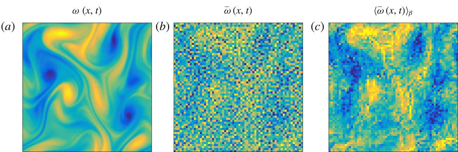
Snapshot of the vorticity field at time  $t=t_{f}/2$. Positive values are shown in blue and negative ones in yellow. Panel (a) is the original vorticity field obtained from the direct numerical simulation with
 $256^{2}$ collocation points. Panel (b) is a fluctuating realisation of the reconstructed vorticity on a
 $64^{2}$ coarse graining with a finite temperature
 $\unicode[STIX]{x1D6FD}^{-1}=1$. Panel (c) is the generalised flow approximation obtained by averaging over the Gibbs ensemble.

The obtained permutation flow provides boundary conditions for the generalised least-action principle. We use the Metropolis algorithm of § 3.2 to reconstruct the velocity field at five intermediate times between  $n\,t_{f}$ and
 $(n+1)\,t_{f}$. Figure 9 illustrates this procedure for
 $n=0$. The vorticity field at time
 $t_{f}$ obtained from the direct simulations is shown in (a). Panel (b) shows a realisation of the reconstructed vorticity
 $\bar{\unicode[STIX]{x1D714}}$ for an inverse temperature
 $\unicode[STIX]{x1D6FD}=1$, and without any averaging. It is obtained by finite differences of the Lagrangian displacement, and one can hardly distinguish any structure. It is only after averaging over
 $10^{6}$ Monte Carlo times that one smears out the noise. The spatial organisation of the original flow is indeed recovered in figure 9(c), which displays the Gibbs-averaged vorticity
 $\langle \bar{\unicode[STIX]{x1D714}}\rangle _{\unicode[STIX]{x1D6FD}}$. The blurry aspect is due to the finite value of temperature. The generalised vorticity will be formally obtained for
 $N_{x},N_{t}\rightarrow \infty$, together with
 $\unicode[STIX]{x1D6FD}\rightarrow \infty$.
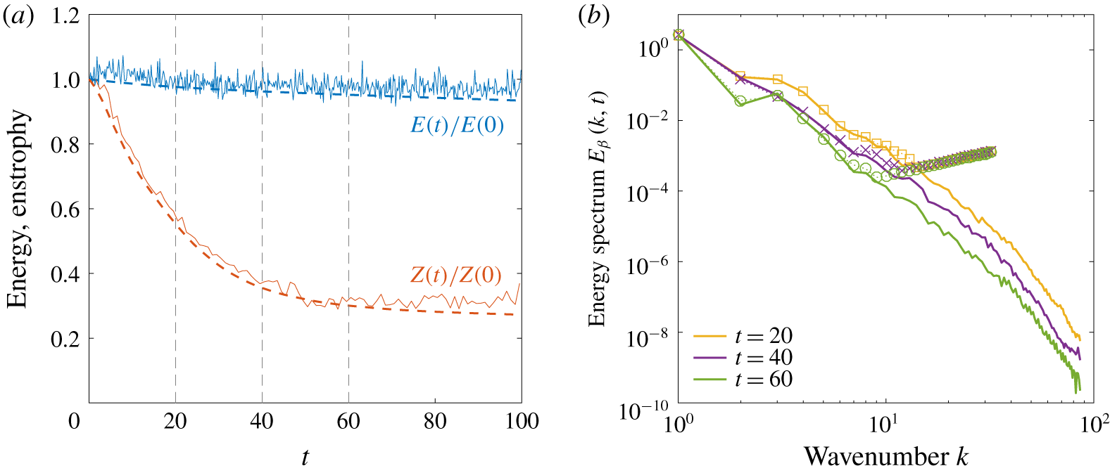
(a) Energy and enstrophy as functions of time both for the actual field (dashed lines) and the reconstructed one (thin solid lines). Here,  $Z(t)$ is averaged over the reconstructed time intervals
 $[n\,t_{f},(n+1)\,t_{f}]$, while
 $E(t)$ is not, whence the stronger fluctuations for the second. Time is here in units of
 $Z^{-1/2}(0)$. (b) Kinetic energy spectra of both the original velocity field (solid lines) and of the reconstructed one (dashed lines with symbols) at different times, as labelled.

This procedure is repeated up to  $n=100$. Figure 10(a) shows the time evolution of the kinetic energy
 $E(t)$ and of the enstrophy
 $Z(t)$. Data from the direct simulation (shown as dashed lines) show that the enstrophy decreases abruptly while energy is almost conserved. This confirms that our settings correspond to the small-viscosity limit of two-dimensional decaying turbulence. The slow decrease of
 $E(t)$ is due to the tiny amount of viscous dissipation used in the numerics. The solid lines are the energy and enstrophy obtained from the reconstructed flow. We observe that the global decay is properly reproduced with superimposed fluctuations due to a finite temperature. Other deviations might be due to statistical errors in the ensemble average or to the discreteness of the reconstructed field. The scaling properties of the velocity fields can be examined from the energy power spectra shown in figure 10(b). Data show an excellent agreement at large scales. As observed earlier in Beltrami flows, reconstructed fields display a
 $\propto k$ range at small scales. The cross-over wavenumber apparently decreases with time, so that one can expect a full thermalisation at large times. The quality of the reconstruction will thus deteriorate, as can be already inferred from (a) at times
 $t\gtrsim 70$.
These attempts at using Brenier’s principle to reconstruct weak solutions to the Euler equations are rather promising. In particular, this approach seems suited to capture irreversible dynamics, and is hence compatible with the concept of dissipative inviscid solutions. Nevertheless, one should be aware that the reconstructed data are here very regular compared to a genuine turbulent three-dimensional flow. While this still constitutes a first step, the observables that we considered are dominated by the larger scales, with a velocity field that apparently remains very close to a classical solution of the inviscid dynamics.
6 Concluding remarks
From a general viewpoint, our analysis highlights one of the limitations of least-action principles when formulated as two-end boundary-value problems in time: they fail to reconstruct vortical dynamics over long time lags. In the solid-rotation example, the issue relates to the final map being likely degenerate, in the sense that can be concomitantly compatible with different equally energetic strong Euler solutions. The critical time  $t_{\star }$ over which this phenomenon happen is naturally interpreted as a turnover time, and is a particular case of Brenier’s general formula (2.9).
Because Brenier’s generalised framework is intrinsically probabilistic, it guarantees the existence of unique minimisers for all times. Yet, the non-deterministic properties of the minimising flows that appear when  $t_{f}\geqslant t_{\star }$ are essentially an artefact of the boundary-value formulation itself. This finding appears unambiguously through the Beltrami example considered in § 4. In the regime
 $t_{f}\geqslant t_{\star }$, the statistical features of the minimising generalised flows are found to be unphysical and therefore unrelated to any kind of turbulent measure. To be used faithfully, it is therefore necessary to restrict the use of the generalised least action principle, and only solve it for short time lags, characterised by
 $t_{f}<t_{\star }$.
In the regime  $t_{f}<t_{\star }$, our work illustrates that Brenier’s generalised least-action principle (2.8) is then not only useful but also versatile. Specifically, our numerics show that it can be efficiently invoke to coarse grain various types of inviscid dynamics in terms of generalised flows, from simple stationary Beltrami dynamic to multi-scale viscous non-stationary two-dimensional turbulence. Coarse-grained statistics for both the Lagrangian trajectories and for the full velocity field can then be reconstructed. Essentially, the generalised framework is practical because it considerably relaxes Arnold’s. Compared to Arnold’s formulation (2.2), the optimisation problem (2.8) is indeed largely unconstrained, and in particular, the probabilistic framework does not rely on any assumption about the smoothness of the minimising flow. This highly desirable feature makes it particularly suitable as a coarse-graining tool, as Brenier’s formulation naturally carries through on discrete settings, both in space and in time – in sharp contrast with Arnold’s formulation based on time-differentiable diffeomorphisms. Besides, the optimising space is sufficiently large, so that minimising algorithms can converge efficiently, without getting trapped within local minima. In the permutation flow viewpoint that we adopted, we note that the number of microscopic configurations to be optimised upon is approximately
 $10^{1025}$, to yield a space–time coarse graining with
 $64^{2}$ grid points and seven time steps. We see this as the main reason why simple Monte Carlo strategies, such as the one presented in § 3, yield faithful approximates to (2.8).
The inviscid dynamics that lies within the scope of Brenier’s action principle includes the strong solutions captured by Arnold’s principle, in which case the minimising generalised flow becomes degenerate as it concentrates on the deterministic solution. More interestingly, the numerical analysis presented in § 5 suggests that Brenier’s principle may also reproduce irreversible dynamics that is a priori prescribed by weak solutions to the Euler equation. While the case of two-dimensional decaying turbulence is peculiar, in the sense that the dynamics is smooth and dominated by large-scale eddies, this numerical evidence is in our view very promising. In particular, it paves the way towards new tools where generalised flows are used to coarse grain truly multi-scale hydrodynamics, including fully developed turbulence.
This overall perspective naturally relies on the crucial assumption that turbulence is described by weak solutions to the Euler equations. If such was indeed the case, generalised flows would then provide a natural framework to think of turbulent solutions in terms of Lagrangian transition probabilities.
Acknowledgements
We thank the Fondation des Treilles for hospitality during the program ‘Irreversibility and Turbulence’, where a prototype version of this paper emerged, and acknowledge K. Ben Saada from the Observatoire de la Côte d’Azur for his continuous sustenance.