


1 Introduction
With growing assets under management, the importance of pension funds as investors increases all around the world. Owing to the design of the social security system and as illustrated in Table 1, in particular the Anglo-Saxon region and – in Continental Europe – the Netherlands and Switzerland are known for their large pension fund markets. The Swiss pension fund market, having a size of USD 732 billion, by asset volume is the seventh largest market worldwide. When measuring the pension fund markets with respect to the countries’ GDP, the Swiss pension fund market was the largest in 2002 and the second largest in 2012. The market represented 118% of the Swiss GDP in 2012. The pension fund markets shown in Table 1 are all growing markets, illustrated by the high compound annual growth rates as well as the increase in proportion of GDP from 2002 to 2012 (with the only exception being South Africa).
Largest pension fund markets

1 Local currency.
2 CAGR = Compound Annual Growth Rate.
Notes: Ranking in brackets.
Source: Tower Watson (2013).
Pension fund markets not only increased in size, but also extended their influence. Several authors, starting with Drucker (Reference Drucker1976) in the 1970s and continued by Clark (Reference Clark2000) in the new century, describe the influence of pension funds on corporate policies. The work was broadened among others by Cronqvist and Fahlenbrach (Reference Cronqvist and Fahlenbrach2009), showing that if US pension funds are blockholders of a company, they significantly influence its investment, financial and compensation policies. A study by Dixon (Reference Dixon2008) brought the topic to the European market by describing recent developments in the French pension system.
With the growing importance of pension funds as investors, the interest with regard to the performance of the funds and the industry as a whole increases. Thereby, we advocate to taking on a comprehensive point of view by considering both the asset and the liability side in performance measurement. Decisions on the asset side, such as the construction of the investment portfolio, can significantly be improved when being in full knowledge with regard to the risk factors on both sides of the balance sheet. In particular, only when measuring the change in market value on both the asset and the liability side, we can assess the effect that a liability matching investment strategy might have.
Whereas the asset side of the balance sheet usually receives large attention in academia and financial practice, the liability side has been considered by fewer authors until today. A range of work has been conducted in the field of asset liability management (ALM). First and foremost is the collected edition by Ziemba and Mulvey (Reference Ziemba and Mulvey1998), containing the most relevant papers on the topic up to that point. A range of further studies were conducted on ALM simulation and the topic of portfolio optimization strategies using an ALM perspective. The first stochastic model for a comprehensive simulation of a pension fund, called ‘Plasm’ (Pension Liability and Asset Simulation Model), was provided by Winklevoss (Reference Winklevoss1982). The model is based on a stochastic asset return and liability simulator and allowed us to analyze a range of future scenarios and strategies. With regard to further information on ALM portfolio optimization strategies, we refer to the studies contributed by Boender (Reference Boender1997), Bogentoft et al. (Reference Bogentoft, Romeijn and Uryasev2001), Kouwenberg (Reference Kouwenberg2001) and Chen et al. (Reference Chen, Yang and Yin2008). The inclusion of liabilities as a benchmark in performance measurement however lacks significant research.
Our contribution to the literature is manifold. First, we build a liability benchmark for pension funds, which is used as an index for referencing the asset performance. Furthermore, by introducing the Asset-Liability-Result (ALR) as performance measure and thus measuring the pension funds’ asset performance with respect to a liability benchmark, we implement a comprehensive performance view that takes into account the pension fund's total balance sheet. In particular, due to the recent drop in yields, the liability benchmark has exhibited a substantial increase in value. The ALR illustrates that the recovery of pension funds from the recent financial crisis took much longer than one would anticipate when looking at the asset side only. We furthermore contribute to the literature by applying the model to the Swiss pension fund market. Analyzing the Swiss pension fund market is important not only due to the significant size of the market, but also because of distinctive features, such as different types of legal guarantees (e.g., minimal conversion rate, minimal investment return, capital guarantees) that cannot be found in other markets. Those legal guarantees lock the plan participants’ claims for benefit at some future point in time in and therefore have a substantial effect on the liability side of the pension funds’ balance sheet. The Swiss application illustrates that the existence of such legal guarantees requires the pension funds to pay close attention to the liability market value and to include the liabilities in performance measurement considerations. When reforming their pension systems, other countries need to be aware of the effects that such legal guarantees have on the liability market value. The introduction of similar social policy instruments will lead to more stringent pension claims and consequently to less flexible liability structures of the pension funds, which finally makes the modeling of the liabilities much more crucial.
We chose two applications. First, we apply the model to the Swiss pension fund market as an aggregate in order to add insights with regard to the performance of the industry as a whole. Second, we calibrate the model for a specific Swiss pension fund, highlighting the added value of the model also in an operational context. By additionally applying the model to a specific pension fund, a robustness check for the overall market is provided. Given the differences in the parameters of the individual pension fund and the overall market (especially with regard to the plan participant structure or the asset distribution), the impact of those differences on the ALR can be analyzed.
The structure of the remaining paper is as follows. Section 2 describes the methodology and highlights in detail, how the model to calculate the ALR (ALR Model) is constructed. Section 3 discusses the data used for both applications, i.e., on one side the calibration to the Swiss pension market and on the other side the calibration to one specific pension fund. Section 4 discusses the results and, finally, Section 5 concludes.
2 Methodology
2.1 The ALR Model
The following section describes the ALR Model, which reproduces the liability side of a pension fund's balance sheet from a mark-to-market perspective. Although this is an everyday procedure for the asset side, the methodology is usually not applied on the liability side. Figure 1 provides a first overview of the ALR Model.
ALR Model summary.
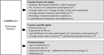
The liabilities are valued with a replicating portfolio approach. The replicating portfolio is constructed as a portfolio of zero-coupon bonds, recreating the payout pattern of a pension fund. To simulate the payout pattern, a range of input variables out of three different categories is required. First, the model requires pension framework inputs, such as the number of active and passive participants (‘passive participants’ refer to the plan participants in payment status, i.e., retirees, persons with disability as well as widows and widowersFootnote 1). Additionally, the model considers the average salary and the average savings per active participant, the average pension of passive participants, the percentage of pension paid out as capital at retirement as well as the contributions made by employees and employers as inputs. Furthermore, several country-specific inputs need to be provided. Those mainly are the discount rates applied (which are discussed further below), information on the expectation of life per age group, the age distribution of the active and passive participants and the yearly increases in salaries and pensions. Last, the ALR Model does also take specific features of the Swiss pension market, such as the age of retirement, the conversion rate,Footnote 2 the minimum plus any additional interest rates on the savingsFootnote 3 and any deductions due to the coordination of different social security schemes, into account. Where necessary, differences between female and male plan participants are incorporated.
Table 2 provides a definition of the parameters included in the model and describes the effects of those parameters on the liability benchmark (ceteris paribus). It is important to note that the described effects always refer to a pension fund that comprises both active participants as well as retirees. If a pension fund would only consist of active participants, some of the implications might not be valid. A change in variable that leads to an increase in the liability duration increases the interest rate sensitivity and therefore also the volatility of the liability benchmark (and vice versa).
Variable description

The input variables are used to calculate the liability value with respect to time t as illustrated in formulas (1)–(6). The formulas show the calculation of the retirement benefits, which represent the largest fraction of pension payments.
First, the expected yearly pension payments of the active (p ta) participants at retirement and the current yearly pension payments for the passive (p tp) participants are calculated.
 $$\eqalign{{\bi p}_t^a & = {\left[ {{{\bi s}_{t - 1}} \times {{(1 + {r_t})}^l} + \mathop \sum \limits_{i = 1}^{\bi l} \left[ {({{\bi w}_i} \times {{(1 + {i^w})}^{i - 1}} - d) \times {{\bi c}_t} \times {{(1 + {r_t})}^{{\bi l} - i}}} \right]} \right]} \times {\bi n}_t^a \cr & \times (1 - o) \times f}$$
 $${\bi p}_t^p = p_t^{av} \times {\bi n}_t^p$$
The variable l accounts for the remaining worklife of the active participants and the vectors (marked in bold) contain the information for the different age groups used in the calculation.
 $${\bi l} = a - {{\bi g}^a}$$
We translate the yearly pension payments into expected cash flows (CF t,m) for different maturities m, which are discounted by the respective discount factor for each maturity (DF t,m). The matrix I takes on a value of either zero or one, indicating the future years, i.e., maturities m, in which the different age groups of active or passive participants obtain a pension. The value of I depends on the age group (ga, gp), the age of retirement (a) and the life expectation (e) of the participants.
 $${\bi C}{{\bi F}_{t,m}} = {\bi p}_t^a \times {(1 + {i^p})^{(m - {\bi l})}} \times {{\bi I}_{t,m}} + {\bi p}_t^p \times {(1 + {i^p})^m} \times {{\bi I}_{t,m}}$$
 $${\bi D}{{\bi F}_{t,m}} = \displaystyle{1 \over {{{(1 + {{\bi y}_{t,m}})}^m}}}$$
The sum of all discounted expected cash flows yields the mark-to-market liability value, which is dependent on time t.
 $${L_t} = \mathop \sum \limits_{m = 0}^M {\bi C}{{\bi F}_{t,m}} \times {\bi D}{{\bi F}_{t,m}}$$
Given the inclusion of those variables, the ALR Model allows the generation of a pension fund specific replicating portfolio. The ALR Model also enables the simulation of entire pension fund markets instead of specific pension funds. This gives us the powerful tool to calculate the pension promises on a mark-to-market basis for entire economies.
With the exception of the discount rates, which are available on a daily basis, the inputs are usually obtainable on a yearly frequency. The liability benchmark will however be calculated on a daily frequency while applying the yearly available inputs on an ex-ante basis. The simultaneous use of daily and yearly frequencies is possible in this setting due to the fact that the yearly available inputs are changing slowly. Some inputs, as for example the retirement age of men, do not change at all during the observation period. The resulting replicating portfolio is therefore rebalanced to the actual liability structure on a yearly basis. During the year, the replicating portfolio's value is behaving according to the movements in discount rates, i.e., in our case the change in the level, slope and curvature of the term structure of interest rates.
2.2 Yield curve model
Since the applied discount rates are the main factors influencing the change in value of the liability benchmark, they warrant further discussion. We use bootstrapped zero yields of Swiss government bonds for the maturities 1–30 years. However, since pension liabilities are characterized by maturities of over 70 years, an extrapolation of yields is conducted. We tested two different theories: a simplistic theory of convergence and the more sophisticated three-factor model by Nelson and Siegel (Reference Nelson and Siegel1987). The theory of convergence uses the simplifying assumption that the term structure of interest rates converges to the 30-year rate. The Nelson–Siegel Model on the other hand is a more sophisticated three-factor model that can be illustrated as follows (Nyholm, Reference Nyholm2008):
 $${y_t}(\tau ) = H \times {\beta _t} + {e_t}$$
β t represents the three yield curve factors: (i) level, (ii) slope and (iii) curvature. The variable e t adds a normally distributed error term to the equation. The factor sensitivities H are represented in the following way, whereby τ determines the maturity and λ represents the speed of time decay:
 $$H = \left[ {\left. {\matrix{ 1 & {\displaystyle{{1 - {\rm exp}( - \lambda {\tau _1})} \over {\lambda {\tau _1}}}} & {\displaystyle{{1 - {\rm exp}( - \lambda {\tau _1})} \over {\lambda {\tau _1}}} - {\rm exp}( - \lambda {\tau _1})} \cr \vdots & \vdots & \vdots \cr 1 & {\displaystyle{{1 - {\rm exp}( - \lambda {\tau _T})} \over {\lambda {\tau _T}}}} & {\displaystyle{{1 - {\rm exp}( - \lambda {\tau _T})} \over {\lambda {\tau _T}}} - {\rm exp}( - \lambda {\tau _T})} \cr } } \right]} \right.$$
A further extension could be implemented by using the four-factor model of Söderlind and Svensson (Reference Söderlind and Svensson1997), whereby the fourth factor represents a second curvature term (representation by Nyholm, Reference Nyholm2008):
 $$H = \left[ {\left. {\matrix{ 1 & {\displaystyle{{1 - {\rm exp}( - {\lambda _1}{\tau _1})} \over {\lambda {\tau _1}}}} & {\displaystyle{{1 - {\rm exp}( - {\lambda _1}{\tau _1})} \over {{\lambda _1}{\tau _1}}} - {\rm exp}( - {\lambda _1}{\tau _1})} & {\displaystyle{{1 - {\rm exp}( - {\lambda _2}{\tau _1})} \over {{\lambda _2}{\tau _1}}} - {\rm exp}( - {\lambda _2}{\tau _1})} \cr \vdots & \vdots & \vdots & \vdots \cr 1 & {\displaystyle{{1 - {\rm exp}( - {\lambda _1}{\tau _T})} \over {\lambda {\tau _T}}}} & {\displaystyle{{1 - {\rm exp}( - {\lambda _1}{\tau _T})} \over {{\lambda _1}{\tau _T}}} - {\rm exp}( - {\lambda _1}{\tau _T})} & {\displaystyle{{1 - {\rm exp}( - {\lambda _2}{\tau _T})} \over {{\lambda _2}{\tau _T}}} - {\rm exp}( - {\lambda _2}{\tau _T})} \cr } } \right]} \right.$$
The fitting process of both models to the yield curve is illustrated in Figures 2 and 3. For illustrative purposes, Figure 2 shows the yield curve of every 50th day in the time period 2003–2013. The dots mark the bootstrapped zero yields obtained from Datastream, whereas the lines show the inter- and extrapolated yield curves. The left graph represents the assumption of convergence to the 30-year rate. The right graph, on the other hand, shows the more sophisticated fitting process applying the three-factor Nelson–Siegel Model.
Yield curve fitting – Convergence Model (left) versus Nelson–Siegel Model (right). Notes: The left graph shows the simplistic Convergence Model (assumes convergence of the yield curve to the 30-year rate). The right graph shows the three-factor Nelson–Siegel Model, which takes into account the level, the slope and the curvature of the whole term structure of interest rates. For illustrative purposes, the graphs show the yield curve of every 50th day in the time period 2003–2013.
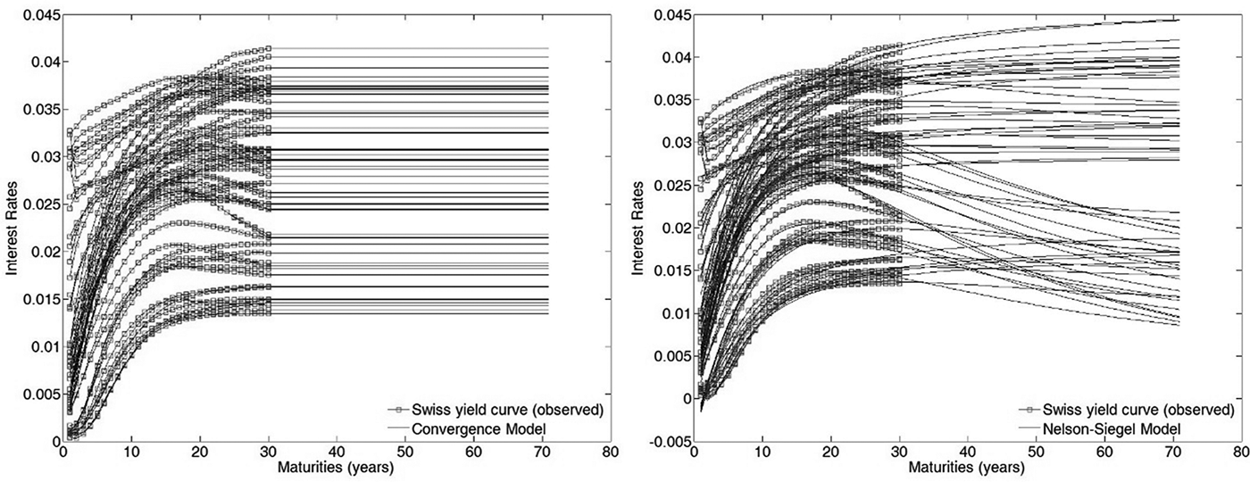
Extrapolation of yield curve – Convergence Model (left) versus Nelson–Siegel Model (right). Notes: The left graph shows the simplistic Convergence Model, whereas the right graph shows the three-factor Nelson–Siegel Model. The graphs show the extrapolated yield curves for the observation period (31.12.2005–31.12.2013) on a daily basis.

Our tests show that the extrapolation models yield similar conclusions with respect to the ALR. Throughout the further discussion, we therefore refrain from showing the results of both extrapolation models and, if not noted otherwise, show the results obtained based on the extrapolation via the Nelson–Siegel Model.
3 Data
We calibrate the ALR Model to the Swiss market based on two different frameworks: first, on an economy-wide level (hereafter called Market Model) and, second, on a pension fund level (hereafter called Pension Fund Model). For the former, we applied the model to the entire Swiss pension fund market. For the latter model, we selected one of the largest Swiss pension funds.Footnote 4 Given the differences in the parameters of the individual pension fund and the overall market, the two applications allow the analysis of the parameter differences and their impact on the ALR.
We make two simplifying assumptions. First, for the Market Model we assume that all Swiss pension funds follow a defined contributionFootnote 5 plan. This assumption is justified, as 85% (in 2004) to 91% (in 2012) of the funds in the market are defined contribution plans. Second, we disregard the splitting of the pension schemes into its mandatory and super-mandatory part. Swiss pension funds are required to insure a person's income only up to a certain fixed amount, which represents the mandatory part of the pension scheme. Insured income above this level falls into the super-mandatory regime and follows other legal requirements, in particular the possibility for pension funds to apply a conversion rate below the statutory fixed rate. We perform robustness checks by applying assumed lower conversion rates, which reflect blended rates for the mandatory and super-mandatory income. Although a lower conversion rate influences the value of the liability benchmark, it does not impact the conclusions drawn in this study. Please refer to Section 4 for the results on the robustness checks.
The replicating portfolio of both data sets takes on a comprehensive view and thus includes pension benefits for retired, disabled and widowed persons. The analysis disregards children pensions due to its small impact. As described in the previous chapter, a broad range of data is required to calculate the liability benchmark. In this section, we will highlight the sources of those variables. An overview of the descriptive statistics is shown in Table 3.
Summary inputs

Notes: This table reports the descriptive statistics of both the Market Model (applied to the Swiss pension market as a whole) and the Pension Fund Model (applied to one of the largest Swiss pension funds). The statistics represent averages over the time period specified.
1 The conversion rate is shown as average over the study period. The conversion rate on the mandatory part of the pension scheme was gradually reduced to currently 6.8%.
3.1 Pension framework inputs
Majority of the pension framework inputs for the Market Model are obtained from the Swiss Federal Statistical Office.Footnote 6 The data required are available for end of year values from 2004 to 2012. Majority of the pension framework inputs for creating the Pension Fund Model are obtained from publicly available annual reports for the time period 2005–2012. We apply the liability setting ex-ante and perform the analysis for both the Market Model and the Pension Fund Model from 31 December 2005 to 31 December 2013.
Bütler and Staubli (Reference Bütler and Staubli2010) estimate cash-out rates in autonomous Swiss pension funds to range from 10% to 30% and in collective funds from 50% to 60%. In 2012, collective funds accounted for 8% of the total number of funds and – owing to their larger size with respect to the number of plan participants per fund – for 26% of the active plan participants and for 15% of the passive plan participants in the Swiss market.Footnote 7 We therefore assumed the average portion of the retirement pension paid out as capital instead of yearly benefits to be at the higher end of the cash-out rates for autonomous funds, i.e., 30%, for both models. However, to account for the even higher rates of collective funds, we run several robustness checks by increasing the cash-out rates stepwise to 60%. Please refer to Section 4 for the results on the robustness checks.
For the Market Model, we do not have average contribution rates of employees and employers and therefore use the statutory defined minimum rates.Footnote 8
3.2 Country-specific inputs
The replicating portfolio is built based on synthetic Swiss government zero-coupon bonds. As discount rates, we therefore use daily bootstrapped zero yields of Swiss government bonds obtained from Datastream and extrapolated with the models described in the previous chapter. We receive the data on life expectation from country-specific life tables published by the WHO.Footnote 9 We then get the age distribution for both the labor force and the retired population, as well as the average age of disabled and widowed persons from the Swiss Federal Statistical Office.Footnote 10 The future average salary increase is calculated from the Swiss Wage Index,Footnote 11 by taking the average historical wage increase over the period analyzed. Last, the future pension payment increases are set to zero. This is based on the fact that retirement benefits are generally not indexed and disability and widow's pension benefits can only be indexed if the financial health of the pension fund allows it.
3.3 Technical inputs
As for the age of retirement, we do not consider early retirement and use the statutory age of 65 for men and 64 for women for observations after 2005 and 63 for women for observations before 2005.Footnote 12 We use the statutory conversion rates, which continuously decreased in the last decade. The minimum interest rate for savings is fixed on a yearly basis by the Federal Council.
3.4 Asset inputs
Furthermore, we require financial market data for modeling the asset side of the Market Model and the Pension Fund Model. The asset side is replicated with nine different asset classes, represented by well-known benchmarks (see Table 4).
Asset classes and benchmarks

Notes: This table reports the benchmarks used for each asset class. The asset class separation reflects the typical classification seen for Swiss pension funds.
All financial market data is obtained from Datastream with a daily frequency (exception: Hedge Fund Index on a monthly frequency). The selected time period corresponds to the time period of the pension framework observations.
Furthermore, we require information about the asset class allocation. For the Market Model, we use the actual total asset distribution across all pension funds at the beginning of the year as a proxy for the strategic asset allocation (SAA). When looking at a single pension fund, as in our Pension Fund Model, we can directly use the SAA published in the annual report. We therefore do not take amendments to the SAA, which have taken place within the year, into account. Figure 4 illustrates the development of the assumed SAA during the study period.
Development of the assumed SAA. Notes: This figure illustrates the development of the asset class distribution. For the Market Model, we use the actual total asset distribution across all pension funds at the beginning of the year as a proxy for the SAA. For the Pension Fund Model, we directly use the SAA published in the annual report. Amendments to the SAA during the year are not taken into account.

4 Results
4.1 Interest rate movements
To understand the development of the replicating portfolio's value, we first need to consider the movements on the interest rate market in the recent decade. Figure 5 illustrates three connected developments based on the Swiss term structure of interest rates. Similar term structure developments can be observed in most developed countries. The figure illustrates several noteworthy points. First, in the graph on the left, we see the falling trend of 2-, 10-, 20- and 30-year interest rates, particularly in the aftermath of the recent financial crisis. The middle graph illustrates the corresponding increase in synthetic prices of zero-coupon bonds. The prices are called synthetic since they have not been observed in the market but were calculated by discounting the cash flows with the zero yield curves. Last, the graph on the right indexes the change in price of zero-coupon bonds of different maturities, starting at an index value of 100 in the beginning of the year 2003. We can see that, due to the long-term discounting effect, in particular the prices of 20- to 30-year zero-coupon bonds increased heavily until 2012. Understanding this significant effect of a drop in long-term interest rates, which are used as discount rates in the valuation of the liabilities, on the price of zero-coupon bonds is crucial for understanding the movement in the replicating portfolio's value discussed in this paper.
Recent development of interest rates and its consequences on the pricing of zero-coupon bonds. Notes: The graph on the left illustrates the falling trend of 2-, 10-, 20- and 30-year interest rates since 2003. The middle graph illustrates the corresponding increase in synthetic prices of zero-coupon bonds (not directly observable in the market). The graph on the right indexes the change in price of zero-coupon bonds starting at an index value of 100 in the beginning of the year 2003.

4.2 The movement of the replicating portfolio
We use the ALR Model to estimate the expected cash flows of the Swiss pension fund market and a specific Swiss pension fund. We assume a horizon as long as the highest expectation of life of the plan participants. In general, this horizon amounts to slightly above 70 years. We do not implement a going concern assumption in our model – rather we are aiming at measuring the currently existing liabilities, which also represents the common approach applied in practice for the valuation of a pension fund's liabilities.
The replicating portfolio then rebuilds the expected pension cash flows over the maximum horizon with synthetic zero-coupon bonds. It thereby takes the specific maturities of the pension liabilities into account. Consequently, also a movement in the slope of the yield curve is reflected by the ALR Model. Since we use synthetic zero-coupon bonds of the Swiss government, we assume maturity-dependent risk-free rates as discount rates. This does not correspond with the valuation of Swiss pension liabilities in reality: pension funds value their liabilities with a single interest rate, which is often related to a combination of the 10-year risk-free rate and a market return, and are thus ignoring the true maturity structure of the liabilities.Footnote 13
Finally, the value of the replicating portfolio is based on the discounted value of the synthetic zero-coupon bonds. In light of this paper's goal, the discounted value of the replicating portfolio is called the liability benchmark. The first row of Figure 6 illustrates the development of the liability benchmark for the two pension frameworks. The indexed liability benchmark reflects the current pension framework structure at any given date; however, it explicitly excludes the yearly changes in the pension framework structure. As an example, the liability benchmark will always take the current number of plan participants and the respective age structure into account. However, at the beginning of every year, the liability benchmark will be rebalanced in order to account for the new number of plan participants and the new age structure. This structural change can lead to a one-time jump in the liability value. Since structural changes are not relevant for performance measurement, they will be excluded in the liability benchmark. As illustration, Figure 6 additionally shows the liability benchmark plus the effect of the structural changes. Furthermore, the second row of the figure shows the movement in the replicating portfolio's modified duration in the course of the study period.
The liability benchmark and the change in duration. Notes: The graphs in the first row illustrate the development of the replicating portfolio's value for the Market Model and the Pension Fund Model – with and without taking structural changes into account. The graphs in the second row show the movement in the replicating portfolio's modified duration with time.

4.3 The ALR
In a next step, we use the liability benchmark as index for the performance on the asset side of the balance sheet. To approximate the asset performance on a daily basis, we use the actual total asset class distribution across all pension funds at the beginning of the year for the Market Model and the SAA for the Pension Fund Model. Based thereon, we calculate the investment portfolio performance.
Figure 7 illustrates the calculated asset performance in the top row and shows that the asset side of the Swiss pension funds has recovered from the financial crisis in 2009, while it reached the pre-crisis peak again in 2010. Furthermore, as illustrated in the middle row of Figure 7, we add the liability benchmark as comparison. We can see that, while the assets decreased in value during the financial crisis, the liabilities of the Swiss pension funds increased due to the substantial drop in interest rates at that time. Although the asset side recovered in 2009, the liabilities continued to increase in value until 2012 based on the ongoing pressure on interest rates.
From the asset performance to the ALR. Notes: The performance of the investment portfolio (asset performance) is illustrated in the graphs of the top row. To approximate the asset performance on a daily basis, we use the actual total asset class distribution across all pension funds at the beginning of the year for the Market Model and the SAA for the Pension Fund Model. The middle row shows both the asset performance and the liability benchmark (without structural changes) in comparison. Finally, the bottom row shows the ALR – i.e., the asset performance measured with respect to the liability benchmark.

Combining these two effects, whereby the asset performance is measured with respect to the liability benchmark, yields the ALR. The liability benchmark (without structural changes) and the asset performance are compared on a daily frequency without applying a weight to either of them. As an alternative, the asset performance and the liability benchmark could be weighted with a funding ratio. However, we refrain from such a procedure in order not to mix up different valuation approaches – which would be required for the introduction of the funding ratio.
The ALR is illustrated in the bottom row of Figure 7. It can be highlighted that the drop in performance during the financial crisis was even higher when it is measured against the liability side. Both the Market Model and the Pension Fund Model illustrate that the Swiss pension market has not recovered from the financial crisis until the end of 2013 when looking at the comprehensive ALR measure. The recovery in 2013 is due to both the increase in long-term interest rates and the positive performance of equity markets in the same year.
4.4 Robustness checks
Given that we disregard the splitting of the pension schemes into its mandatory and super-mandatory part, we perform robustness checks on the assumed conversion rate. In the standard model, we used the statutory minimum conversion rates, which averaged at 7.1% over the study period. Pension funds that provide benefits beyond the statutory minimum are allowed to apply a lower conversion rate. The average blended conversion rate from 2006 to 2013 for the mandatory and the super-mandatory regimes amounted to 6.7%, whereas the average minimum value amounted to 5.6%.Footnote 14 We run the model with both alternative assumptions and thereby provide a lower bandwidth of possible outcomes. Figure 8 illustrates that the modified duration of the liabilities decreases with a lower conversion rate, whereas the ALR exhibits a slightly less volatile development. However, given the limited impact on the ALR, it does not impact the conclusions drawn in this study.
Conversion rate robustness check. Notes: The figure shows the different results dependent on the assumptions with respect to the conversion rate. The graphs illustrate the model for assumed average conversion rates of 7.1% (standard model), 6.7% (average blended conversion rate 2006–2013) and 5.6% (minimum blended conversion rate 2006–2013). The graphs in the first row show the movement in the replicating portfolio's modified duration with time. The second row shows the ALR – i.e., the asset performance measured with respect to the liability benchmark.

Based on Bütler and Staubli (Reference Bütler and Staubli2010), we assumed a capital option percentage (cash-out rate) of 30%. Since collective pension funds exhibit higher cash-out rates ranging from 50% to 60%, we perform robustness checks on this parameter by increasing it stepwise to 40%, 50% and 60%. Although the pension fund analyzed in the Pension Fund Model is an autonomous fund, we apply the higher cash-out rates to allow for comparison between the two calibrations. Figure 9 shows the results with respect to the modified duration and the ALR. The graphs highlight that, with increasing cash-out rates, the duration of the liabilities decreases substantially. Similar to the robustness check with respect to lower conversion rates, higher cash-out rates lead to an ALR that exhibits a slightly less volatile development. However, although the effect is observable, it does not impact the conclusions drawn in this study.
Capital option percentage (cash-out rate) robustness check. Notes: The figure shows the different results dependent on the assumptions with respect to the capital option percentage (cash-out rate). The graphs illustrate the model for assumed average cash-out rates of 30% (standard model), 40%, 50% and 60%. The graphs in the first row show the movement in the replicating portfolio's modified duration with time. The second row shows the ALR – i.e., the asset performance measured with respect to the liability benchmark.

4.5 Yearly ALR analysis
Table 5 finally shows the yearly performance and risk analysis of the investment portfolio and the liability benchmark as well as the resulting ALR time series. The risk analysis shows the yearly standard deviation and 99% daily value at risk. It clearly highlights the substantial influence of including the liability side as a benchmark in the analysis both on the return and on the risk side. In 6 out of the 8 years analyzed, the liability benchmark and the asset performance moved in opposite directions. This stems from the fact that historically, interest rates most often decreased when financial markets performed poorly (and vice versa). Pension funds therefore must be aware that during financial market downturns, they should not only be concerned about the negative effect on the asset side, but also about the disadvantageous development with respect to the liabilities. Furthermore, the risk analysis illustrates that the liability benchmark is more volatile and has a higher downside risk than the asset performance. This characteristic is caused by the interest rate volatility coupled with the high duration of the liabilities. Liabilities with an average duration of 20–25 years (as in our model) move strongly even when interest rates change only slightly.
Yearly ALR analysis

Notes: The table shows the annual return, the annualized volatility and the 99% daily value at risk of the liability benchmark and the asset performance as well as the resulting ALR time series for the Market Model (MM) and the Pension Fund Model (PFM). The annualized return of the ALR is calculated based on the yearly returns of the liability and the asset benchmark. The full period annualized returns for the liability benchmark, the asset performance and the ALR are calculated based on the geometric average of the respective yearly returns from 2006 to 2013. The value at risk is calculated based on the historical time series. A year is assumed to have 252 trading days.
The Pension Fund Model exhibits a substantially lower ratio of active participants towards passive participants – indicating the higher proportion of benefit recipients. A higher proportion of passive participants results in a reduced average duration of the pension liabilities. A lower duration finally leads to the fact that the Pension Fund Model exhibits lower volatility and lower downside risk in the liability benchmark than the Market Model. On the other hand, the Pension Fund Model is based on a slightly riskier asset allocation (due to a higher equity allocation), which results in higher volatility and downside risk of the asset performance. The overall effect on the volatility and downside risk of the ALR is therefore mixed.
When looking at the return measures of 2008, the impact of the financial crisis on both the asset performance as well as the liability benchmark can be observed. According to the model, the average asset performance of Swiss pension funds in the crash year amounted to −12.2%. However, given the parallel decrease in interest rate, the liability market value increased by 42.5%. Measuring the relative performance of the assets with respect to the liability benchmark then results in an ALR of −54.7% – which clearly illustrates the underestimation of the effect of the recent financial crisis on the pension funds’ financial situation.
Based on the results discussed in this chapter, we see the ALR as a comprehensive performance measure, taking a mark-to-market perspective for the entire balance sheet. Current performance measures focus entirely on the asset performance. However, we illustrate that the usage of the liability side as benchmark adds additional insight for the performance and risk analysis. This is in particular true for pension funds and other financial institutions having highly long-term liabilities.
5 Conclusion
We illustrated how to build a replicating portfolio for the liabilities of a pension fund and an entire pension market and highlighted its merits when using it as a benchmark for referencing the asset performance. In particular, due to the drop in yields since the recent financial crisis, the liability benchmark for Swiss pension funds has exhibited a substantial increase in value. Combining the liability and the asset performance illustrated that the recovery from the recent financial crisis took much longer than one would anticipate when looking at the asset side only.
We strongly advocate to using a comprehensive performance measure such as the ALR in two areas: Firstly when analyzing the performance of entire pension fund markets and secondly as operational tool for pension funds. Decisions on the asset side, such as the construction of the investment portfolio, can be improved when being in the full knowledge with regard to the risk factors on both sides of the balance sheet. In particular, only when looking at a comprehensive result, such as provided by the ALR, we can see the effect that a liability matching investment strategy might have.
The ALR Model is meant to be a starting point for further analyses in the field of ALM for pension funds. We see added value in a broad range of topics. The ALR Model can be extended in its ability to serve as performance measurement tool. It can be refined even more to a specific fund by calibration with internal information (for example, using the actual age distribution) and more frequent data points (for example, quarterly reports).
Another stream of literature being targeted with the ALR Model is the area of portfolio rebalancing. At the moment, mainly value-based rebalancing strategies can be observed in the market. Some academic work is currently being done in the field of risk contribution rebalancing strategies (see Kohler and Wittig, Reference Kohler and Wittig2014). A further extension targeted with the ALR Model is the implementation of an Asset-Liability-Rebalancing approach.
Furthermore, the model can be used as market model to analyze various pension markets around the world. By this means, we are able to highlight the development of the pension promises over the recent years and to calculate the large increase in the liability value due to the recent interest rate fall (see Novy-Marx and Rauh, Reference Novy-Marx and Rauh2011).
We also see potential in further studies surrounding the discount rates applied, given their huge impact on the value of the liabilities. It might be worthwhile to discuss whether applying the risk-free rate to pension payments is justifiable or whether an alternative approach would be warranted.



