1. Introduction
A granular fluid describes a collection of discrete, solid, macroscopic particles that collide and interact through energy-loss mechanisms, such as friction and inelastic collisions. As such, granular fluids are dissipative systems. The particles are large enough so that, unlike molecules and smaller nano-sized particles (Talbot et al. Reference Talbot, Cheng, Schefer and Willis1980), they are not affected by thermal fluctuations. The lower size limit for particles in a granular fluid is usually assumed to be of the order of a micrometre (Andreotti, Forterre & Pouliquen Reference Andreotti, Forterre and Pouliquen2013). There does not appear to be an upper size limit as long as the number of interacting particles is large enough.
Granular fluids and gaseous fluids differ in important ways. Collisions among granular particles are inelastic, unlike molecular gases, in which collisions are almost always fully elastic. These inelastic particle collisions can lead to granular clustering because, with inelastic collisions, the relative motion between the particles decreases (Brilliantov & Pöschel Reference Brilliantov and Pöschel2004). This can lead to behaviour where a ‘Maxwell’s demon’ effectively operates in granular systems. For example, particles in a shaken box may cluster to one side, leaving the other side evacuated (Van der Weele Reference Van der Weele2008). Granular media can also behave like a gas, liquid or solid depending on how the particles are packed and the amount of kinetic energy input. Understanding and developing models for many of the interesting phenomena related to granular media are now heavily researched topics.
In the past, efforts were made to develop models for the multiphase flow of coupled gas and granular fluids because of their importance for practical problems, such as coal combustors (Zhou et al. Reference Zhou, Zhao, Duan, Qu and Chen2011), catalytic bed reactors (Zimmermann & Taghipour Reference Zimmermann and Taghipour2005), biomass gasification (Gerber, Behrendt & Oevermann Reference Gerber, Behrendt and Oevermann2010), particle hoppers (Srivastava & Sundaresan Reference Srivastava and Sundaresan2003), scouring sand underneath submerged pipes (Zhao & Fernando Reference Zhao and Fernando2007) and pyroclastic flows (Neri et al. Reference Neri, Ongaro, Macedonio and Gidaspow2003). A number of methods have been developed to study these essentially low-speed incompressible flow problems (as described in § 2).
High-speed, compressible, dense granular multiphase flows occur in a wide range of scenarios, including dust explosions in coal mines (Sapko et al. Reference Sapko, Weiss, Cashdollar and Zlochower2000; Zheng et al. Reference Zheng, Feng, Jing, Qian, Li, Liu and Huang2009), grain elevators, food processing and storage facilities, volcanic eruptions (Wilson Reference Wilson1980), dust layers lifted by shocks (Zydak & Klemens Reference Zydak and Klemens2007; Chuanjie et al. Reference Chuanjie, Baiquan, Bingyou, Qian and Yidu2012; Wayne et al. Reference Wayne, Vorobieff, Smyth, Bernard, Corbin, Maloney, Conroy, White, Anderson and Kumar2013), dust in natural gas explosions (Liu et al. Reference Liu, Hu, Bai and Chen2013) and interior ballistics (Koo & Kuo Reference Koo and Kuo1977; Markatos & Kirkcaldy Reference Markatos and Kirkcaldy1983; Markatos Reference Markatos1986; Porterie & Loraud Reference Porterie and Loraud1994; Nussbaum et al. Reference Nussbaum, Helluy, Hérard and Carriére2006). Although these are extremely important problems, much less work has been done to formulate models that consistently cover the range from dilute to dense particle packing in the presence of high-speed gas flows and shock waves. There are a few notable exceptions, such as the models by Fan et al. (Reference Fan, Chen, Jiang and Li2007), Chuanjie et al. (Reference Chuanjie, Baiquan, Bingyou, Qian and Yidu2012) and Khmel’ & Fedorov (Reference Khmel’ and Fedorov2015).
Consider an example of where high-speed compressible granular multiphase flows are important, that of layered coal-dust explosions (Houim & Oran Reference Houim and Oran2015 a ,Reference Houim and Oran b ). Here we are interested in knowing the behaviour of particles and their interactions with a high-speed background flow. This flow can sweep up and entrain particles that are initially in densely packed layers and then distribute these particles as a diluted mixture of particles and gas. Such flows may be highly turbulent and laden with shocks. To further complicate matters, the particles may react chemically, agglomerate or fragment (Dacombe et al. Reference Dacombe, Pourkashanian, Williams and Yap1999). We need to know the controlling physical processes in such scenarios and how they affect the particle distribution and background flow. To achieve this, we need a model for a granular flow that interacts with a compressible background gas. This model must include enough of the physics for the background gas, the granular media and the coupling interactions between them to provide physically accurate predictions over a wide range of granular packing and background flow conditions.
Solving for the behaviour of such complex, heterogeneous flows is difficult because it is necessary to formulate a model that includes enough of the physics of a compressible gas, the particles and the interactions among these, and to develop numerical procedures that will handle inherent difficulties in solving this coupled model. In this paper, we first describe such a model and a solution approach that gives reasonable results when compared to theoretical limits and experiments, and so it is a start for solving the problems of coupled compressible flows with gas and granular material.
2. Background
One type of multiphase model for coupled gas and granular flows is described by a set of equations based on the kinetic theory of granular flow (Lun et al.
Reference Lun, Savage, Jeffrey and Chepurniy1984; Gidaspow Reference Gidaspow1994). These models describe the interaction of a molecular gas with an inelastic granular fluid (Brilliantov & Pöschel Reference Brilliantov and Pöschel2004) made up of many incompressible particles. In this type of formulation, granular fluids are characterized by a granular temperature (
 ${\it\Theta}_{s}$
), representing the random translational kinetic energy of the particles. The granular temperature is used in constitutive relations to compute a ‘solids pressure’ (
 $p_{s}$
) that describes an intergranular stress resulting from particle collisions. The solids pressure for the granular phase is analogous to the usual pressure for the gas phase. Friction forces between colliding particles can become substantial when the volume fraction of particles (
 ${\it\alpha}_{s}$
) is high, which results in a large frictional–collisional pressure (
 $p_{fric}$
) (Johnson & Jackson Reference Johnson and Jackson1987). This type of granular–gas multiphase fluid model can be considered as a two-fluid model (Ishii & Hibiki Reference Ishii and Hibiki2006). There are many methods for solving these equations for low-speed flows, as reviewed in Van Wachem et al. (Reference Van Wachem, Schouten, van den Bleek, Krishna and Sinclair2001). There are now several existing numerical codes for simulating low-speed granular multiphase flows (such as MFIX (Syamlal, Rogers & O’Brien Reference Syamlal, Rogers and O’Brien1993)).
Many compressible granular multiphase flows are modelled using the ‘dust–gas approximation’, which neglects particle–particle interactions and collision processes, and so it effectively assumes that the particles are dilute in the background gas (Collins et al. Reference Collins, Ferguson, Chien, Kuhl, Krispin and Glaz1994; Benkiewicz & Hayashi Reference Benkiewicz and Hayashi2002; Saito, Marumoto & Takayama Reference Saito, Marumoto and Takayama2003; Pelanti & LeVeque Reference Pelanti and LeVeque2006; Fedorov, Kharlamova & Khmel’ Reference Fedorov, Kharlamova and Khmel’2007; Kuhl, Bell & Beckner Reference Kuhl, Bell and Beckner2010). These models have been used to study detonations of particle suspensions, explosion suppression from aerosolized particles, lifting of dilute dust layers, and the dispersion and combustion of aluminium particles in the turbulent flow field generated by an explosion. They are not applicable when there are dense particle clusters, which could occur when dense dust layers are lifted by shocks (Fan et al. Reference Fan, Chen, Jiang and Li2007), or in coalmine explosions, where settled layers of dust may accumulate to volume fractions of the order of 47 % (Edwards & Ford Reference Edwards and Ford1988). When the dust is dense, the effects of particle–particle interactions must be included.
When the volume fraction of particles is very high, it becomes necessary to use other types of models, such as the Baer–Nunziato (BN) equations (Baer & Nunziato Reference Baer and Nunziato1986), the Nigmatulin equations (Nigmatulin Reference Nigmatulin1990) or Eulerian interior ballistic models (Koo & Kuo Reference Koo and Kuo1977; Markatos & Kirkcaldy Reference Markatos and Kirkcaldy1983; Markatos Reference Markatos1986; Porterie & Loraud Reference Porterie and Loraud1994; Nussbaum et al. Reference Nussbaum, Helluy, Hérard and Carriére2006). The BN equations were developed to describe high-pressure combustion processes, such as detonation of high-explosive charges, where particle compression and distortion are significant. The BN equations are a variant of the ‘seven-equation model’ presented by Saurel & Abgrall (Reference Saurel and Abgrall1999), in which the interfacial velocity and pressure are chosen to be the particle velocity and gas-phase pressure, respectively. The BN model relaxes the particle incompressibility assumption used in the kinetic-theory approach mentioned above, but adds an advection equation for the solid volume fraction. Neglecting phase change, this equation is often written as
 $$\begin{eqnarray}\frac{\partial {\it\alpha}_{s}}{\partial t}+\boldsymbol{v}_{s}\boldsymbol{\cdot }\boldsymbol{{\rm\nabla}}{\it\alpha}_{s}=0,\end{eqnarray}$$
where
 ${\it\alpha}_{s}$
and
 $\boldsymbol{v}_{s}$
are the volume fraction and velocity vector for the solid-phase particles, respectively. This new equation is written in a non-conservative form, and, as such, changes the physical nature of compression waves in the solid phase from that predicted by kinetic-theory models. That is, granular-phase compression waves in the BN equations represent pressure waves moving through the solid material itself and, as a result, the volume fraction changes only at solid contact surfaces. The volume fraction equation for kinetic-theory-based models (assuming constant particle density and neglecting phase change) is
 $$\begin{eqnarray}\frac{\partial {\it\alpha}_{s}}{\partial t}+\boldsymbol{{\rm\nabla}}\boldsymbol{\cdot }{\it\alpha}_{s}\boldsymbol{v}_{s}=0,\end{eqnarray}$$
which has very different wave propagation properties from the volume fraction equation for BN models. Granular-phase compression waves for kinetic-theory-based models are produced by particle collisions that create compaction waves and granular shocks (Kamenetsky et al. Reference Kamenetsky, Goldshtein, Shapiro and Degani2000). These granular compaction waves and shocks, in turn, change the volume fraction of particles rather than the material density of the particles themselves. The BN equations, as a result, are more appropriate for highly packed (i.e. the particle volume fraction is at or above the random close-packing limit) granular mixtures at high pressures with constant compressive contact between the grains (Lhuillier, Chang & Theofanous Reference Lhuillier, Chang and Theofanous2013). Therefore, the use of BN-type models is physically inappropriate for looser granular flow regimes, where the particles are not in constant compressive contact and intergranular stress results from collisions and friction between the grains, which are the focus of this paper.
Interior gun ballistic models (Koo & Kuo Reference Koo and Kuo1977; Markatos & Kirkcaldy Reference Markatos and Kirkcaldy1983; Markatos Reference Markatos1986; Porterie & Loraud Reference Porterie and Loraud1994; Nussbaum et al.
Reference Nussbaum, Helluy, Hérard and Carriére2006) involve high particle loadings, high pressures (of the order of 1000 atm or more) and high-speed flow. Particle compression and deformation can be significant under these conditions. Nevertheless, interior ballistic models often assume incompressible particles. The intergranular stress for these models lacks the formalism of the kinetic-theory approach. They often describe intergranular stress through empirical correlations that are similar to some frictional–collisional pressure models. As a result, many interior ballistic models can be derived from the more formal kinetic-theory multiphase equations by assuming zero granular temperature (
 ${\it\Theta}_{s}$
) and that the intergranular stress is based solely on a type of frictional–collisional pressure. A multiphase approach similar to interior ballistic models has been used by Rogue et al. (Reference Rogue, Rodriguez, Haas and Saurel1998) to simulate shocks interacting with dense particle curtains.
A limitation of all continuum (or Eulerian) particle models is that they become physically invalid when the number of particles in a computational cell is low and the continuum assumption fails. Under these conditions, the particles act discretely and Lagrangian models, which track individual particles or groups of particles, could be more appropriate. Lagrangian methods can also be used to model the particles in dense granular flow (Helland, Occelli & Tadrist Reference Helland, Occelli and Tadrist2000; Nusca, Horst & Newill Reference Nusca, Horst and Newill2004; Ling et al. Reference Ling, Wagner, Beresh, Kearney and Balachandar2012; Capecelatro & Desjardins Reference Capecelatro and Desjardins2013). These models can be computationally expensive when there are a large number of particles or groups to track. They are also expensive when particle collision rules have to be applied, as occurs when the granular phase approaches the packing limit.
The approach described in this paper is to couple a continuum kinetic-theory granular model to a compressible gas. The primary focus is on mixtures of granular particles and compressible gas, for which the particle packing can range from very dilute, so that particles do not interact with each other, to densely packed conditions, in which friction and collisions become significant. It is assumed that the particle packing and gas-phase pressure are not so high that elastic waves propagating through the solid material and particle deformation need to be considered.
2.1. Solution difficulties
The underlying difficulties in developing an accurate set of governing equations for coupled gas and granular flow are based on the difficulties of representing important physical interactions, some of which are not defined as clearly as they are for single-phase gaseous flows. This is the topic addressed in the next section (§ 3) on model formulation. Once we have such a model, there remains the issue of how we can use and adapt existing numerical simulation tools to solve specific problems of interest, and what new issues arise from the formulation. In the case of coupled gas–granular flows, the underlying new difficulties are essentially physical, but these also have counterparts in how the solutions must be implemented numerically.
The difficulties in actually solving the equations shown below in § 3 result from a combination of non-conservative interphase coupling terms and numerical stiffness in dilute and dense granular regions. More specifically, we need to deal with: (1) non-conservative ‘nozzling’ terms (Schwendeman, Wahle & Kapila Reference Schwendeman, Wahle and Kapila2006; Karni & Hernández-Dueñas Reference Karni and Hernández-Dueñas2010; Crochet & Gonthier Reference Crochet and Gonthier2013) arising from variations of the particle volume fraction within a control volume; (2) a
 $pDV$
work term that affects the gas as particles enter and leave a control volume (Abgrall & Karni Reference Abgrall and Karni2010); (3) hyperbolic degeneracy when the intergranular stress in the granular phase is zero; (4) stiffness of the intergranular stress in highly packed regions; and (5) potential loss of hyperbolicity from complex-valued wave speeds.
When the pressure is uniform and the background fluid is stationary (zero velocity), the gas-phase momentum equations with a variation of particle volume fraction reduce to the ‘non-disturbing condition’ (Saurel & Abgrall Reference Saurel and Abgrall1999),
 $$\begin{eqnarray}\boldsymbol{{\rm\nabla}}{\it\alpha}_{g}p_{g}=p_{g}\boldsymbol{{\rm\nabla}}{\it\alpha}_{g}.\end{eqnarray}$$
Here
 ${\it\alpha}_{g}$
is the gas-phase volume fraction,
 $p_{g}$
is the gas-phase pressure, and the term on the right-hand side is the ‘nozzling term’ due to its analogy with the
 $pDA$
term in the quasi-one-dimensional gas dynamic nozzle flow equations. Computing the left- and right-hand sides of equation (2.3) independently (Toro Reference Toro, A. and B.1989; Nussbaum et al.
Reference Nussbaum, Helluy, Hérard and Carriére2006) can lead to situations where, for purely numerical reasons, the terms may not balance. This induces unphysical flow and pressure oscillations that can cause numerical solutions to fail (Liou et al.
Reference Liou, Chang, Nguyen and Theofanous2008).
Another complication is that the compaction wave speed of the particles (analogous to the sound speed of a gas) ranges between zero, when
 ${\it\Theta}_{s}$
is zero or at low particle volume fractions, and approaches infinity at the packing limit. If the compaction wave speed is zero, the result is a pressureless granular gas (sometimes called ‘sticky particle’ models (LeVeque Reference LeVeque2004)), which causes numerical problems (specifically, hyperbolic degeneracy (Pelanti & LeVeque Reference Pelanti and LeVeque2006)). This means that characteristic-based methods, such as many weighted essentially non-oscillatory (WENO) schemes (Balsara & Shu Reference Balsara and Shu2000), or the standard piecewise parabolic method (PPM) (Colella & Woodward Reference Colella and Woodward1984) cannot be used to solve these equations in a straightforward manner. Godunov-based methods would require a Riemann solver for the granular phase that is valid in the pressureless state and transitions to a high-pressure state. Despite hyperbolic degeneracy, approximate Riemann solvers were previously designed for pressureless dust (Collins et al.
Reference Collins, Ferguson, Chien, Kuhl, Krispin and Glaz1994; Pelanti & LeVeque Reference Pelanti and LeVeque2006), but not for kinetic-theory-based granular models.
The intergranular stress is extremely sensitive to even very small fluctuations of solid volume fraction in dense regions that approach the packing limit. This makes it difficult to develop solution approaches that are both low-dissipation (high-order) and robust. A difficulty arises because the volume fraction of particles influences the gas and granular phases differently. Particles restrict the area where fluid can flow, and so they accelerate the gas by a nozzling term. On the other hand, the volume fraction controls the compressibility of the granular phase in the same way that density does for the gas phase.
To deal with these numerical problems, the coupled system of equations may be solved using highly dissipative numerical methods. In these cases, refining the grid or using any high-order (therefore more accurate) numerical methods can trigger instabilities that can be masked by excessive numerical diffusion (Nussbaum et al.
Reference Nussbaum, Helluy, Hérard and Carriére2006). Recent methods appear to have overcome this for the BN equations (Karni & Hernández-Dueñas Reference Karni and Hernández-Dueñas2010; Crochet & Gonthier Reference Crochet and Gonthier2013). Another solution method, used in interior ballistics, is to split the gas and granular conservation equations and solve a Riemann problem for each phase independently and then to compute the non-conservative nozzling and
 $pDV$
coupling terms separately (Toro Reference Toro, A. and B.1989), but this approach can violate the non-disturbing condition.
Now high-order, low-dissipation methods for solving the compressible Euler and Navier–Stokes equations are becoming widespread due, in part, to their excellent properties for describing shock waves and compressible turbulence (Grinstein, Margolin & Rider Reference Grinstein, Margolin and Rider2007; Thornber et al. Reference Thornber, Mosedale, Drikakis, Youngs and Williams2008; Poludnenko & Oran Reference Poludnenko and Oran2010, Reference Poludnenko and Oran2011). The nonlinear filtering effect and added dissipation near sharp gradients that is inherent in shock capturing schemes acts, in many ways, like the explicit filtering and subgrid turbulence models used in traditional large-eddy simulation. In addition, the turbulence in many high-speed shock-laden flows is non-Kolmogorov (Oran & Gamezo Reference Oran and Gamezo2007), that is, inhomogeneous, non-isotropic and driven by shock–shock interactions and Richtmyer–Meshkov and Rayleigh–Taylor instabilities. Physically accurate subgrid turbulence models usually do not exist for such conditions. Often the only choice in these situations is to use implicit large-eddy simulation, which requires low-dissipation numerical algorithms (Grinstein et al. Reference Grinstein, Margolin and Rider2007; Thornber et al. Reference Thornber, Mosedale, Drikakis, Youngs and Williams2008).
This presents an interesting quandary for multiphase models based on kinetic theory or any other multiphase model where the particles are supposed to be subgrid. In such models, the computational cell size is limited by the particle diameter. It is necessary to have enough particles in a computational cell so that the granular phase can be represented as some kind of fluid. Thus, there are grid limitations on the size of the finest mesh. This limiting computational cell size may be too coarse to capture features of the gas phase, such as the viscous sublayer of a turbulent boundary layer.
In this paper, we first present a model that solves two sets of Euler equations, one for the gas phase and one for the particles, with coupling terms that connect them. We then show how the two sets of equations can be solved using a high-order, low-dissipation numerical method. The technique uses components from existing Riemann solvers and edge interpolation schemes, and incorporates a relatively small modification to the AUSM
 $^{+}$
-up flux (Liou Reference Liou1996, Reference Liou2006) for the granular phase. The fluxes and computed states obtained from solving the gas- and granular-phase Riemann problems are assembled to form the convective fluxes and non-conservative terms. Tests of the method that show its ability to preserve the non-disturbing condition, compute multiphase shock-tube problems and simulate strong shocks interacting with dense layers of dust are discussed. Finally, we present comparisons from this model to experimental measurements of shock and particle-curtain interactions (Rogue et al.
Reference Rogue, Rodriguez, Haas and Saurel1998; Ling et al.
Reference Ling, Wagner, Beresh, Kearney and Balachandar2012; Wagner et al.
Reference Wagner, Beresh, Kearney, Trott, Castaneda, Pruett and Baer2012) and transmitted oblique granular shocks and granular contact surfaces in layers of dust (Fan et al.
Reference Fan, Chen, Jiang and Li2007). In future papers, we will discuss extensions that include effects of granular viscosity and heat and mass diffusion, which are not included in this paper.
3. Model formulation
The equations that couple a compressible gas to granular particles are presented. Details, such as proving that the mixture mass, momentum and energy equations are fully conservative, derivation of the entropy equations for each phase, and a hyperbolicity analysis of the model equations, are given in appendix A.
3.1. Euler equations for a single-phase, multispecies flow
The Euler equations for a multicomponent, reacting, compressible gas flow with
 $N_{g}$
chemical species can be written as
 $$\begin{eqnarray}\displaystyle & \displaystyle \frac{\partial {\it\rho}}{\partial t}+\boldsymbol{{\rm\nabla}}\boldsymbol{\cdot }({\it\rho}\boldsymbol{v})=0, & \displaystyle\end{eqnarray}$$
 $$\begin{eqnarray}\displaystyle & \displaystyle \frac{\partial {\it\rho}Y_{j}}{\partial t}+\boldsymbol{{\rm\nabla}}\boldsymbol{\cdot }({\it\rho}Y_{j}\boldsymbol{v})=\dot{{\bf\omega}}_{j},\quad j=1,\ldots ,N_{g}, & \displaystyle\end{eqnarray}$$
 $$\begin{eqnarray}\displaystyle & \displaystyle \frac{\partial {\it\rho}\boldsymbol{v}}{\partial t}+\boldsymbol{{\rm\nabla}}\boldsymbol{\cdot }({\it\rho}\boldsymbol{v}\boldsymbol{v})+\boldsymbol{{\rm\nabla}}p={\it\rho}\boldsymbol{g}, & \displaystyle\end{eqnarray}$$
 $$\begin{eqnarray}\displaystyle & \displaystyle \frac{\partial {\it\rho}E}{\partial t}+\boldsymbol{{\rm\nabla}}\boldsymbol{\cdot }[\boldsymbol{v}({\it\rho}E+p)]={\it\rho}\,\boldsymbol{g}\boldsymbol{\cdot }\boldsymbol{v}, & \displaystyle\end{eqnarray}$$
 $Y_{j}$
,
 ${\it\rho}$
,
 $p$
,
 $T$
,
 $E$
,
 $\boldsymbol{v}$
and
 $\boldsymbol{g}$
are the mass fraction of species
 $j$
, density, pressure, temperature, total energy, velocity components and gravitational acceleration vector, respectively. The homogeneous reaction rate due to chemical reactions is denoted by
 $\dot{{\bf\omega}}_{j}$
.
The ideal gas equation of state is used to relate the pressure, chemical composition, temperature and density of the gas phase,
 $$\begin{eqnarray}p={\it\rho}R_{u}T\mathop{\sum }_{j=1}^{N_{g}}\frac{Y_{j}}{M_{j}},\end{eqnarray}$$
where
 $M_{j}$
is the molecular weight of species
 $j$
and
 $R_{u}$
is the universal gas constant. The total energy of the gas phase,
 $E$
, is given by
 $$\begin{eqnarray}E=H-\frac{p}{{\it\rho}}=\mathop{\sum }_{j=1}^{N}Y_{j}\left(h_{f\,j}^{0}+\int _{T_{0}}^{T}C_{Pj}(s)\,\text{d}s\right)-\frac{p}{{\it\rho}}+\frac{\boldsymbol{v}\boldsymbol{\cdot }\boldsymbol{v}}{2},\end{eqnarray}$$
where
 $H$
is the total enthalpy,
 $h_{f\,j}^{0}$
is the enthalpy of formation at reference temperature
 $T_{0}$
and
 $C_{Pj}$
is the constant-pressure specific heat of species
 $j$
. Thermodynamic data may be taken from a number of sources. Here data are taken from Goos, Burcat & Rusnic (Reference Goos, Burcat and Rusnic2010). The sound speed,
 $c$
, is given by
 $$\begin{eqnarray}c^{2}={\it\gamma}\frac{p}{{\it\rho}},\end{eqnarray}$$
where
 ${\it\gamma}$
is the ratio of specific heats.
3.2. Euler equations for a gas in a multiphase flow
Now we modify (3.1)–(3.4) so they can be used to describe the gas phase in the gas–granular multiphase problem by accounting for the volume taken up by the particles through the gas-phase volume fraction
 ${\it\alpha}_{g}$
(Ishii & Hibiki Reference Ishii and Hibiki2006),
 $$\begin{eqnarray}\displaystyle & \displaystyle \frac{\partial {\it\alpha}_{g}{\it\rho}_{g}}{\partial t}+\boldsymbol{{\rm\nabla}}\boldsymbol{\cdot }({\it\alpha}_{g}{\it\rho}_{g}\boldsymbol{v}_{g})=S^{M}, & \displaystyle\end{eqnarray}$$
 $$\begin{eqnarray}\displaystyle & \displaystyle \frac{\partial {\it\alpha}_{g}{\it\rho}_{g}Y_{g,j}}{\partial t}+\boldsymbol{{\rm\nabla}}\boldsymbol{\cdot }({\it\alpha}_{g}{\it\rho}_{g}Y_{g,j}\boldsymbol{v}_{g})={\it\alpha}_{g}\dot{{\bf\omega}}_{g,j}+S_{g,j}^{Y},\quad j=1,\ldots ,N_{g}, & \displaystyle\end{eqnarray}$$
 $$\begin{eqnarray}\displaystyle & \displaystyle \frac{\partial {\it\alpha}_{g}{\it\rho}_{g}\boldsymbol{v}_{g}}{\partial t}+\boldsymbol{{\rm\nabla}}\boldsymbol{\cdot }({\it\alpha}_{g}{\it\rho}_{g}\boldsymbol{v}_{g}\boldsymbol{v}_{g})+\boldsymbol{{\rm\nabla}}{\it\alpha}_{g}p_{g}=p_{int}\boldsymbol{{\rm\nabla}}{\it\alpha}_{g}+{\it\alpha}_{g}{\it\rho}_{g}\boldsymbol{g}+\boldsymbol{S}^{\boldsymbol{p}}, & \displaystyle\end{eqnarray}$$
 $$\begin{eqnarray}\displaystyle & \displaystyle \frac{\partial {\it\alpha}_{g}{\it\rho}_{g}E_{g}}{\partial t}+\boldsymbol{{\rm\nabla}}\boldsymbol{\cdot }[{\it\alpha}_{g}\boldsymbol{v}_{g}({\it\rho}_{g}E_{g}+p_{g})]=-p_{int}\frac{\partial {\it\alpha}_{g}}{\partial t}+{\it\alpha}_{g}{\it\rho}_{g}\boldsymbol{g}\boldsymbol{\cdot }\boldsymbol{v}_{g}+S_{g}^{E}, & \displaystyle\end{eqnarray}$$
 $g$
refers to the gas. An important new variable here is
 ${\it\alpha}_{g}$
, the volume fraction occupied by the gas, so that
 $$\begin{eqnarray}{\it\alpha}_{g}+{\it\alpha}_{s}=1\quad \text{and}\quad \boldsymbol{{\rm\nabla}}{\it\alpha}_{g}=-\boldsymbol{{\rm\nabla}}{\it\alpha}_{s},\end{eqnarray}$$
where
 ${\it\alpha}_{s}$
is the volume fraction of particles. The quantities
 $Y_{g,j}$
,
 ${\it\rho}_{g}$
,
 $p_{g}$
,
 $T_{g}$
,
 $E_{g}$
and
 $\boldsymbol{v}_{g}$
are the mass fraction of species
 $j$
, density, pressure, temperature, total energy and velocity vector of the gas, respectively. The pressure at the gas–solid interface around the particles,
 $p_{int}$
, is used in the nozzling (
 $p_{int}\boldsymbol{{\rm\nabla}}{\it\alpha}_{g}$
) and
 $pDV$
work (
 $-p_{int}(\partial {\it\alpha}_{g}/\partial t)$
) terms. The reaction rate due to homogeneous chemical reactions is denoted by
 $\dot{{\bf\omega}}_{g,j}$
. Additional interphase coupling terms describing transfer of mass, momentum and energy between the gas and the particles are denoted by
 $S^{M}$
,
 $S_{g,j}^{Y}$
,
 $\boldsymbol{S}^{\boldsymbol{p}}$
and
 $S_{g}^{E}$
. These are described in § 3.5.
3.3. Euler equations for the particulate phase in a multiphase flow
These equations are similar in form to the Euler equations for the gas phase (Gidaspow Reference Gidaspow1994). The main difference is that compressibility is introduced by changes in solid volume fraction rather than the material density of the particles, so that compaction waves (analogous to acoustic waves, rarefactions and shocks in a molecular gas) travelling through granular media directly change the particle volume fraction,
 ${\it\alpha}_{s}$
. The granular-phase governing equations for mass, momentum, pseudo-thermal energy (PTE) and internal energy with
 $N_{s}$
species within each particle are
 $$\begin{eqnarray}\displaystyle & \displaystyle \frac{\partial {\it\alpha}_{s}{\it\rho}_{s}}{\partial t}+\boldsymbol{{\rm\nabla}}\boldsymbol{\cdot }({\it\alpha}_{s}{\it\rho}_{s}\boldsymbol{v}_{s})=-S^{M}, & \displaystyle\end{eqnarray}$$
 $$\begin{eqnarray}\displaystyle & \displaystyle \frac{\partial {\it\alpha}_{s}{\it\rho}_{s}Y_{s,j}}{\partial t}+\boldsymbol{{\rm\nabla}}\boldsymbol{\cdot }({\it\alpha}_{s}{\it\rho}_{s}Y_{s,j}\boldsymbol{v}_{s})={\it\alpha}_{s}\dot{{\bf\omega}}_{s,j}+S_{s,j}^{Y},\quad j=1,\ldots ,N_{s}, & \displaystyle\end{eqnarray}$$
 $$\begin{eqnarray}\displaystyle & \displaystyle \frac{\partial {\it\alpha}_{s}{\it\rho}_{s}\boldsymbol{v}_{s}}{\partial t}+\boldsymbol{{\rm\nabla}}\boldsymbol{\cdot }({\it\alpha}_{s}{\it\rho}_{s}\boldsymbol{v}_{s}\boldsymbol{v}_{s})+\boldsymbol{{\rm\nabla}}p_{s}+\boldsymbol{{\rm\nabla}}p_{fric}=-\boldsymbol{{\rm\nabla}}{\it\alpha}_{s}p_{g}-p_{int}\boldsymbol{{\rm\nabla}}{\it\alpha}_{g}+{\it\alpha}_{s}{\it\rho}_{s}\boldsymbol{g}-\boldsymbol{S}^{\boldsymbol{p}}, & \displaystyle\end{eqnarray}$$
 $$\begin{eqnarray}\displaystyle & \displaystyle \frac{\partial {\it\alpha}_{s}{\it\rho}_{s}E_{s}}{\partial t}+\boldsymbol{{\rm\nabla}}\boldsymbol{\cdot }({\it\alpha}_{s}{\it\rho}_{s}E_{s}\boldsymbol{v}_{s})=-p_{s}\boldsymbol{{\rm\nabla}}\boldsymbol{\cdot }\boldsymbol{v}_{s}+S_{s}^{PTE}, & \displaystyle\end{eqnarray}$$
 $$\begin{eqnarray}\displaystyle & \displaystyle \frac{\partial {\it\alpha}_{s}{\it\rho}_{s}e_{s}}{\partial t}+\boldsymbol{{\rm\nabla}}\boldsymbol{\cdot }({\it\alpha}_{s}{\it\rho}_{s}e_{s}\boldsymbol{v}_{s})=S_{s}^{E}, & \displaystyle\end{eqnarray}$$
 $p_{s}$
,
 $p_{fric}$
,
 $e_{s}$
,
 $E_{s}$
and
 $\dot{{\it\gamma}}$
are the solids pressure derived from kinetic theory, frictional–collisional pressure, internal energy, PTE and dissipation of
 $E_{s}$
due to inelastic particle collisions, respectively. The homogeneous reaction rate of granular species
 $i$
is denoted by
 $\dot{{\it\omega}}_{s,i}$
. The additional interphase coupling terms,
 $S_{s,j}^{Y}$
,
 $S_{s}^{PTE}$
and
 $S_{s}^{E}$
, are discussed in § 3.5.
The PTE,
 $E_{s}$
, represents the energy due to random translational motion of the particles,
 $$\begin{eqnarray}E_{s}={\textstyle \frac{3}{2}}{\it\Theta}_{s}.\end{eqnarray}$$
It is a function of the granular temperature,
 ${\it\Theta}_{s}$
, defined as the mean square of the particle velocity fluctuations. The granular temperature is usually presented in units of
 $\text{m}^{2}~\text{s}^{-2}$
rather than K (Gidaspow Reference Gidaspow1994; Van Wachem et al.
Reference Van Wachem, Schouten, van den Bleek, Krishna and Sinclair2001; Brilliantov & Pöschel Reference Brilliantov and Pöschel2004).
The ‘normal’ temperature of the particles,
 $T_{s}$
, is determined from the solid sensible internal energy,
 $e_{s}$
, through
 $$\begin{eqnarray}e_{s}=\mathop{\sum }_{j=1}^{N_{s}}Y_{s,j}\left(e_{f\,j}^{0}+\int _{T_{0}}^{T_{s}}C_{V,s,j}(s)\,\text{d}s\right),\end{eqnarray}$$
where
 $N_{s}$
is the number of species in the solid phase,
 $e_{f\,j}^{0}$
is an internal energy of formation and
 $C_{V,s,j}$
is the constant-volume specific heat of species
 $j$
in the particle phase. This equation assumes that the temperature distribution within each particle is uniform, and so the Biot modulus is small. More complex equations that include the effect of non-uniform temperature distributions inside the particles could be used if the Biot number were large (Koo & Kuo Reference Koo and Kuo1977; Markatos & Kirkcaldy Reference Markatos and Kirkcaldy1983; Nussbaum et al.
Reference Nussbaum, Helluy, Hérard and Carriére2006). (Note that the granular temperature,
 ${\it\Theta}_{s}$
, is not related to ‘normal’ temperature
 $T_{s}$
.)
The density of the solid particles is given by
 $$\begin{eqnarray}{\it\rho}_{s}=\mathop{\sum }_{j=1}^{N_{s}}Y_{s,j}{\it\rho}_{s,j}(T_{s}),\end{eqnarray}$$
where
 ${\it\rho}_{s,j}$
is the density of species
 $j$
. In this paper, we take
 ${\it\rho}_{s}$
to be constant. Relaxing this assumption will be a topic of future work.
The solids pressure,
 $p_{s}$
, represents collisional effects of the particles and is given by an equation of state for a granular gas (Gidaspow Reference Gidaspow1994),
 $$\begin{eqnarray}p_{s}={\it\alpha}_{s}{\it\rho}_{s}{\it\Theta}_{s}[1+2(1+e){\it\alpha}_{s}g_{0}],\end{eqnarray}$$
where
 $e$
is the coefficient of restitution. The radial distribution function,
 $g_{0}$
, is defined by (Gidaspow Reference Gidaspow1994)
 $$\begin{eqnarray}\frac{1}{g_{0}}=1-\left(\frac{{\it\alpha}_{s}}{{\it\alpha}_{s,max}}\right)^{1/3},\end{eqnarray}$$
where
 ${\it\alpha}_{s,max}$
is the packing limit, which is an input parameter commonly set to 0.65 (Agrawal et al.
Reference Agrawal, Loezos, Syamlal and Sundaresan2001; Igci et al.
Reference Igci, Andrews, Sundaresan, Pannala and O’Brien2008), which is representative of the random close-packing limit of uniform spheres (Andreotti et al.
Reference Andreotti, Forterre and Pouliquen2013). Other expressions for
 $g_{0}$
and
 $p_{s}$
could be used (see e.g. Kamenetsky et al.
Reference Kamenetsky, Goldshtein, Shapiro and Degani2000; Van Wachem et al.
Reference Van Wachem, Schouten, van den Bleek, Krishna and Sinclair2001).
When particles occupy a high volume fraction, frictional–collisional pressure must be added to
 $p_{s}$
to describe pressure-like forces that arise as layers of granular material slide over each other. The inclusion of frictional–collisional pressure has the effect of limiting compaction when
 ${\it\Theta}_{s}$
approaches zero. In highly packed conditions, the binary collision assumption in the Boltzmann equation, which is used to derive the granular-phase equation of state and transport properties, becomes invalid since particles are in contact with several other particles. In these conditions, high rates of inelastic particle collisions can rapidly reduce
 ${\it\Theta}_{s}$
to zero. This results in
 $p_{s}=0$
, which allows particles to pack to unphysically high levels. In such dense regions, frictional–collisional pressure is needed to provide the intergranular stress necessary to limit compaction. In this work we use the correlation of Johnson & Jackson (Reference Johnson and Jackson1987),
 $$\begin{eqnarray}p_{fric}=\left\{\begin{array}{@{}ll@{}}0\quad & \text{if }{\it\alpha}_{s}<{\it\alpha}_{s,crit},\\ 0.1{\it\alpha}_{s}\displaystyle \frac{({\it\alpha}_{s}-{\it\alpha}_{s,crit})^{2}}{({\it\alpha}_{s,max}-{\it\alpha}_{s})^{5}}\quad & \text{if }{\it\alpha}_{s}\geqslant {\it\alpha}_{s,crit},\end{array}\right.\end{eqnarray}$$
where
 ${\it\alpha}_{s,crit}$
is 0.5 unless otherwise noted and
 $p_{fric}$
is in units of Pa. Other expressions for frictional–collisional pressure could be used as well (Koo & Kuo Reference Koo and Kuo1977; Markatos & Kirkcaldy Reference Markatos and Kirkcaldy1983; Jenike Reference Jenike1987; Gidaspow Reference Gidaspow1994; Saurel & Abgrall Reference Saurel and Abgrall1999; Van Wachem et al.
Reference Van Wachem, Schouten, van den Bleek, Krishna and Sinclair2001; Nussbaum et al.
Reference Nussbaum, Helluy, Hérard and Carriére2006; Ling et al.
Reference Ling, Wagner, Beresh, Kearney and Balachandar2012; Schneiderbauer, Aigner & Pirker Reference Schneiderbauer, Aigner and Pirker2012). Here the sum of the solids and frictional–collisional pressures is called the total intergranular stress,
 $$\begin{eqnarray}p_{s,tot}=p_{s}+p_{fric},\end{eqnarray}$$
to avoid ambiguity with the terminology used for interior ballistics.
(Another approach to limiting compaction of the solid phase is to limit the minimum granular temperature near the packing limit (Kamenetsky et al.
Reference Kamenetsky, Goldshtein, Shapiro and Degani2000). This approach, while seemingly ad hoc, has a physical basis. The coefficient of restitution,
 $e$
, is not a constant, as assumed in many kinetic-theory granular multiphase models, but is a function of impact velocity. Higher impact velocities (higher
 ${\it\Theta}_{s}$
) convert more PTE,
 $E_{s}$
, into internal energy,
 $e_{s}$
, through viscoelastic deformation (Brilliantov & Pöschel Reference Brilliantov and Pöschel2004). Collisions become increasingly elastic (
 $e\rightarrow 1$
) as the granular temperature decreases. This effect limits both the rate at which
 ${\it\Theta}_{s}$
can decrease and its lower value. Recent granular gas models account for this to some extent (Brilliantov & Pöschel Reference Brilliantov and Pöschel2004), but, to our knowledge, these have not been used in multiphase flow calculations.)
We do not include the mean kinetic energy in the conservation equation for PTE (equation (3.16)). This avoids small truncation errors of kinetic energy, which can lead to unphysical values of
 $E_{s}$
. Dissipation of
 $E_{s}$
due to inelastic particle collisions (see § 3.5) often reduces
 $E_{s}$
to the point where it is small compared to the mean kinetic energy,
 $\boldsymbol{v}_{s}\boldsymbol{\cdot }\boldsymbol{v}_{s}/2$
. In a numerical solution of these equations, small errors in the mean kinetic energy can cause small fluctuations of
 ${\it\Theta}_{s}$
, which, in dense-particle regimes, produces severe oscillations of
 $p_{s}$
and
 $p_{fric}$
. Such oscillations can degrade calculations to the point of failure. Decoupling kinetic energy from the PTE equation makes the numerical algorithm more robust. A similar approach is often used in astrophysical calculations (e.g. ASC FLASH Center (2012)). Developing a numerical algorithm that allows us to put the kinetic energy in the PTE equation while maintaining robustness is a topic of ongoing research.
The pressure term in the
 $E_{s}$
equation (3.16) does not include flow work from frictional–collisional pressure. This is consistent from a thermodynamics point of view. The
 $p_{fric}$
models used here are analogous to a barotropic equation of state for a fluid. It is possible to show, using thermodynamic arguments, that the total energy equation for a barotropic fluid simplifies to the mechanical energy equation (see appendix A). Performing a similar analysis for granular mixtures reveals that only the solids pressure,
 $p_{s}$
, contributes to changes in
 $E_{s}$
from compression and expansion (changes in volume fraction) of the particles. If the mean kinetic energy were included in the definition of
 $E_{s}$
, the friction pressure would enter the total PTE equation (3.18) as
 $\boldsymbol{v}_{s}\boldsymbol{\cdot }\boldsymbol{{\rm\nabla}}p_{fric}$
, while the solids pressure would be present in the usual manner,
 $\boldsymbol{{\rm\nabla}}\boldsymbol{\cdot }(\boldsymbol{v}_{s}p_{s})$
(see (A 9)).
The Euler equations for the granular particles are compressible, similar to those for the gas phase. One key difference, mentioned above, is that this compressibility manifests itself through changes in particle volume fraction in the form of compaction waves. This granular-compaction wave speed can be derived for the particulate phase in the same way that the sound speed can be derived for a real gas (Serna & Marquina Reference Serna and Marquina2005). The compaction wave speed for a general granular gas, where friction pressure is only a function of
 ${\it\alpha}_{s}$
, is
 $$\begin{eqnarray}c_{s}^{2}=\frac{1}{{\it\rho}_{s}}\left[\left.\frac{\partial p_{s}^{tot}}{\partial {\it\alpha}_{s}}\right|_{{\it\Theta}_{s}}+\frac{2}{3}\frac{{\it\Theta}_{s}\left(\left.\displaystyle \frac{\partial p_{s}^{tot}}{\partial {\it\Theta}_{s}}\right|_{{\it\alpha}_{s}}\right)^{2}}{{\it\rho}_{s}{\it\alpha}_{s}^{2}}\right].\end{eqnarray}$$
Then by using the definitions for
 $p_{s}$
and
 $p_{fric}$
(see (3.21) and (3.23)), we find
 $$\begin{eqnarray}c_{s}^{2}={\it\Theta}_{s}(A+{\textstyle \frac{2}{3}}A^{2}+{\it\alpha}_{s}B)+c_{fric}^{2},\end{eqnarray}$$
where
 $$\begin{eqnarray}A=1+2(1+e){\it\alpha}_{s}g_{0},\quad B=2(1+e)(g_{0}+{\it\alpha}_{s}g_{0}^{\prime }),\quad g_{0}^{\prime }=\frac{g_{0}^{2}}{3{\it\alpha}_{s,max}}\left(\frac{{\it\alpha}_{s,max}}{{\it\alpha}_{s}}\right)^{2/3}\!.\quad\end{eqnarray}$$
The frictional contribution to the compaction wave speed (in MKS units) is
 $$\begin{eqnarray}c_{fric}^{2}=\left\{\begin{array}{@{}ll@{}}0\quad & \text{if }{\it\alpha}_{s}<{\it\alpha}_{s,crit},\\ \displaystyle \frac{1}{{\it\rho}_{s}}\frac{({\it\alpha}_{s}-{\it\alpha}_{s,crit})}{({\it\alpha}_{s,max}-{\it\alpha}_{s})^{5}}\left[{\it\alpha}_{s}\left(\frac{1}{5}+\frac{1}{2}\frac{{\it\alpha}_{s}-{\it\alpha}_{s,crit}}{{\it\alpha}_{s,max}-{\it\alpha}_{s}}\right)+\frac{{\it\alpha}_{s}-{\it\alpha}_{s,crit}}{10}\right]\quad & \text{if }{\it\alpha}_{s}\geqslant {\it\alpha}_{s,crit}.\end{array}\right.\end{eqnarray}$$
Several models are available for
 $p_{s}$
,
 $p_{fric}$
and
 $g_{0}$
, as mentioned above (see e.g. Kamenetsky et al.
Reference Kamenetsky, Goldshtein, Shapiro and Degani2000; Van Wachem et al.
Reference Van Wachem, Schouten, van den Bleek, Krishna and Sinclair2001; Nussbaum et al.
Reference Nussbaum, Helluy, Hérard and Carriére2006). Typically, the coefficient of restitution,
 $e$
, the random close-packing limit,
 ${\it\alpha}_{s,max}$
, and the threshold volume fractions above which
 $p_{fric}$
becomes non-zero,
 ${\it\alpha}_{s,crit}$
, are input parameters. Exploring alternative intergranular stress models and the influence of input parameters is ongoing work.
3.4. The nozzling and
 $pDV$
work terms

In granular multiphase flows, it is common to choose
 $p_{int}=p_{g}$
(Gidaspow Reference Gidaspow1994). If we further assume that the particle density (
 ${\it\rho}_{s}$
) is not a function of pressure or intergranular stress, the
 $pDV$
work term reduces to
 $$\begin{eqnarray}-p_{int}\frac{\partial {\it\alpha}_{g}}{\partial t}=p_{g}\frac{\partial {\it\alpha}_{s}}{\partial t}=-p_{g}\boldsymbol{{\rm\nabla}}\boldsymbol{\cdot }{\it\alpha}_{s}\boldsymbol{v}_{s}-p_{g}\frac{S^{M}}{{\it\rho}_{s}}.\end{eqnarray}$$
With these expressions, the final momentum equations for the gas and granular phase are
 $$\begin{eqnarray}\displaystyle & \displaystyle \frac{\partial {\it\alpha}_{g}{\it\rho}_{g}\boldsymbol{v}_{g}}{\partial t}+\boldsymbol{{\rm\nabla}}\boldsymbol{\cdot }({\it\alpha}_{g}{\it\rho}_{g}\boldsymbol{v}_{g}\boldsymbol{v}_{g})+\boldsymbol{{\rm\nabla}}{\it\alpha}_{g}p_{g}=p_{g}\boldsymbol{{\rm\nabla}}{\it\alpha}_{g}+{\it\alpha}_{g}{\it\rho}_{g}\boldsymbol{g}+\boldsymbol{S}^{\boldsymbol{p}}, & \displaystyle\end{eqnarray}$$
 $$\begin{eqnarray}\displaystyle & \displaystyle \frac{\partial {\it\alpha}_{s}{\it\rho}_{s}\boldsymbol{v}_{s}}{\partial t}+\boldsymbol{{\rm\nabla}}\boldsymbol{\cdot }({\it\alpha}_{s}{\it\rho}_{s}\boldsymbol{v}_{s}\boldsymbol{v}_{s})+\boldsymbol{{\rm\nabla}}p_{s}+\boldsymbol{{\rm\nabla}}p_{fric}=-{\it\alpha}_{s}\boldsymbol{{\rm\nabla}}p_{g}+{\it\alpha}_{s}{\it\rho}_{s}\boldsymbol{g}-\boldsymbol{S}^{\boldsymbol{p}}, & \displaystyle\end{eqnarray}$$
 $$\begin{eqnarray}\frac{\partial {\it\alpha}_{g}{\it\rho}_{g}E_{g}}{\partial t}+\boldsymbol{{\rm\nabla}}\boldsymbol{\cdot }[{\it\alpha}_{g}\boldsymbol{v}_{g}({\it\rho}_{g}E_{g}+p_{g})]=-p_{g}\boldsymbol{{\rm\nabla}}\boldsymbol{\cdot }{\it\alpha}_{s}\boldsymbol{v}_{s}+{\it\alpha}_{g}{\it\rho}_{g}\boldsymbol{g}\boldsymbol{\cdot }\boldsymbol{v}_{g}+S_{g}^{E},\end{eqnarray}$$
where the
 $pDV$
work associated with phase change is absorbed into
 $S_{g}^{E}$
.
3.5. Interphase coupling terms
Source terms that couple the governing equations for the gas and granular phases (aside from the nozzling and
 $pDV$
work terms) include drag, convective heat transfer, phase change and dissipation of PTE from inelastic collisions, and lifting forces. We neglect the virtual mass and Basset (history) forces (even though they can be important when computing particle trajectories in some high-speed applications (Ling, Haselbacher & Balachandar Reference Ling, Haselbacher and Balachandar2011
a
,Reference Ling, Haselbacher and Balachandar
b
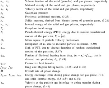
)). Selected variable definitions and the source terms and their physical meaning are given in table 1.
Abbreviated list of variables and their physical interpretation.

The mass exchange term due to phase change is
 $$\begin{eqnarray}S^{M}={\dot{M}},\end{eqnarray}$$
where the total mass rate of phase change is
 $$\begin{eqnarray}{\dot{M}}=\mathop{\sum }_{i=1}^{N_{g}}S_{g,i}^{Y}=-\mathop{\sum }_{i=1}^{N_{s}}S_{s,i}^{Y},\end{eqnarray}$$
and
 $S_{g,i}^{Y}$
and
 $S_{s,i}^{Y}$
are the mass rates of production for species
 $i$
for the gas and granular phases due to phase change. The momentum source terms resulting from phase change, drag and lift are
 $$\begin{eqnarray}\boldsymbol{S}^{\boldsymbol{p}}=\boldsymbol{f}_{Drag}+\boldsymbol{f}_{Lift}+\boldsymbol{v}_{int}{\dot{M}}.\end{eqnarray}$$
The drag force for the particulate mixture is given by the correlation of Gidaspow (Reference Gidaspow1994),
 $$\begin{eqnarray}\boldsymbol{f}_{Drag}=K_{sg}(\boldsymbol{v}_{s}-\boldsymbol{v}_{g}),\end{eqnarray}$$
where
 $$\begin{eqnarray}K_{sg}=\left\{\begin{array}{@{}ll@{}}0.75C_{d}\displaystyle \frac{{\it\rho}_{g}{\it\alpha}_{g}{\it\alpha}_{s}|\boldsymbol{v}_{s}-\boldsymbol{v}_{g}|}{d_{s}{\it\alpha}_{g}^{2.65}}\quad & \text{if }{\it\alpha}_{g}\geqslant 0.8,\\ \displaystyle 150\frac{{\it\alpha}_{s}^{2}{\it\mu}_{g}}{{\it\alpha}_{g}d_{s}^{2}}+1.75\frac{{\it\rho}_{g}{\it\alpha}_{s}|\boldsymbol{v}_{g}-\boldsymbol{v}_{s}|}{d_{s}}\quad & \text{if }{\it\alpha}_{g}<0.8,\end{array}\right.\end{eqnarray}$$
the drag coefficient,
 $C_{d}$
, is
 $$\begin{eqnarray}C_{d}=\left\{\begin{array}{@{}ll@{}}\displaystyle 24({\it\alpha}_{g}Re)^{-1}[1+0.15({\it\alpha}_{g}Re)^{0.687}]\quad & \text{if }{\it\alpha}_{g}Re<1000,\\ 0.44\quad & \text{if }{\it\alpha}_{g}Re\geqslant 1000,\end{array}\right.\end{eqnarray}$$
and the Reynolds number is defined by
 $$\begin{eqnarray}Re=\displaystyle \frac{{\it\rho}_{g}|\boldsymbol{v}_{g}-\boldsymbol{v}_{s}|d_{s}}{{\it\mu}_{g}}.\end{eqnarray}$$
Other forms of the drag coefficient are available in the literature (Syamlal et al. Reference Syamlal, Rogers and O’Brien1993; Van Wachem et al. Reference Van Wachem, Schouten, van den Bleek, Krishna and Sinclair2001; Parmar, Haselbacher & Balachandar Reference Parmar, Haselbacher and Balachandar2010), and should be tested, but this is not the subject of this paper
The lift force,
 $\boldsymbol{f}_{Lift}$
, is modelled using the Magnus lift force defined by
 $$\begin{eqnarray}\boldsymbol{f}_{Lift}=C_{l}{\it\alpha}_{s}{\it\rho}_{g}(\boldsymbol{v}_{s}-\boldsymbol{v}_{g})\times (\boldsymbol{{\rm\nabla}}\times \boldsymbol{v}_{g}),\end{eqnarray}$$
where the lift coefficient,
 $C_{l}$
, has a value of 0.5 (Drew & Lahey Reference Drew and Lahey1987). The influence of the Saffman lift force is currently neglected.
The interfacial velocity used for momentum exchange and energy during phase change are defined using the value from the phase that is losing mass,
 $$\begin{eqnarray}\boldsymbol{v}_{int}=\left\{\begin{array}{@{}ll@{}}\boldsymbol{v}_{s}\quad & \text{if }{\dot{M}}>0,\\ \boldsymbol{v}_{g}\quad & \text{if }{\dot{M}}<0.\end{array}\right.\end{eqnarray}$$
The source terms in the energy equations are
 $$\begin{eqnarray}\displaystyle & \displaystyle S_{g}^{E}=-q_{conv}+{\it\phi}_{visc}-{\it\phi}_{slip}+E_{g,int}{\dot{M}}+(\boldsymbol{f}_{Drag}+\boldsymbol{f}_{Lift})\boldsymbol{\cdot }\boldsymbol{v}_{s}, & \displaystyle\end{eqnarray}$$
 $$\begin{eqnarray}\displaystyle & \displaystyle S_{s}^{E}=q_{conv}-e_{s,int}{\dot{M}}+\dot{{\it\gamma}}, & \displaystyle\end{eqnarray}$$
 $$\begin{eqnarray}\displaystyle & \displaystyle S_{s}^{PTE}=-\dot{{\it\gamma}}-{\it\phi}_{visc}+{\it\phi}_{slip}-E_{s,int}{\dot{M}}, & \displaystyle\end{eqnarray}$$
 $E_{g,int}=H_{g,int}-p_{int}/{\it\rho}_{s}$
. These energy exchange terms include, in addition to convective heat transfer, effects from dissipation of PTE from inelastic particle collisions (
 $\dot{{\it\gamma}}$
), dissipation of PTE due to viscous effects of particles being immersed in a fluid (
 ${\it\phi}_{visc}$
), and production of PTE due to drag forces (
 ${\it\phi}_{slip}$
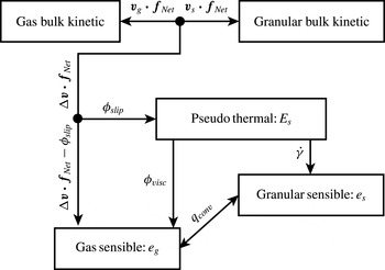
). The relationship between these energy exchange mechanisms is shown in figure 1.
Relationship between the energy transfer mechanisms modelled in the source terms to the energy equations, where
 $\boldsymbol{f}_{Net}=\boldsymbol{f}_{Drag}+\boldsymbol{f}_{Lift}$
and
 ${\rm\Delta}\boldsymbol{v}=\boldsymbol{v}_{s}-\boldsymbol{v}_{g}$
.

The convective heat flux between the gas and particles is
 $$\begin{eqnarray}q_{conv}=6\frac{{\it\alpha}_{s}{\it\lambda}_{g}Nu}{d_{s}^{2}}(T_{g}-T_{s}),\end{eqnarray}$$
where the Nusselt number is estimated using the correlation of Gunn (Reference Gunn1978),
 $$\begin{eqnarray}Nu=(7-10{\it\alpha}_{g}+5{\it\alpha}_{g}^{2})(1+0.7Re^{0.2}Pr_{g}^{1/3})+(1.33-2.4{\it\alpha}_{g}+1.2{\it\alpha}_{g}^{2})Re^{0.7}Pr_{g}^{1/3},\end{eqnarray}$$
and
 $Pr_{g}$
is the gas-phase Prandtl number.
The model for viscous damping of PTE is adopted from Gidaspow (Reference Gidaspow1994),
 $$\begin{eqnarray}{\it\phi}_{visc}=3K_{sg}{\it\Theta}_{s}.\end{eqnarray}$$
The rate of internal energy production into the gas phase due to frictional heating during particle acceleration is
 $$\begin{eqnarray}q_{Drag}={\rm\Delta}\boldsymbol{v}\boldsymbol{\cdot }\boldsymbol{f}_{Net},\end{eqnarray}$$
where
 $\boldsymbol{f}_{Net}=\boldsymbol{f}_{Drag}+\boldsymbol{f}_{Lift}$
and
 ${\rm\Delta}\boldsymbol{v}=\boldsymbol{v}_{s}-\boldsymbol{v}_{g}$
. Not all of this internal energy heats the gas as it flows around the particles. Some of this heating is diverted into producing random translational motion (PTE) of the particles. The production rate of PTE during particle acceleration,
 ${\it\phi}_{slip}$
, is given by Koch & Sangani (Reference Koch and Sangani1999) with their correction factor fixed at unity,
 $$\begin{eqnarray}{\it\phi}_{slip}=\frac{81{\it\alpha}_{s}{\it\mu}_{g}^{2}}{g_{0}d_{s}^{3}{\it\rho}_{s}\sqrt{{\rm\pi}}}\frac{|\boldsymbol{v}_{g}-\boldsymbol{v}_{s}|^{2}}{\sqrt{{\it\Theta}_{s}}}.\end{eqnarray}$$
Alternative models for
 ${\it\phi}_{slip}$
could also be used (e.g. Koch & Sangani Reference Koch and Sangani1999), but again these are not the subject of this paper.
The granular dissipation model adopted for this study (Lun et al. Reference Lun, Savage, Jeffrey and Chepurniy1984) is a variant of Haff’s cooling law (Haff Reference Haff1983; Brilliantov & Pöschel Reference Brilliantov and Pöschel2004),
 $$\begin{eqnarray}\dot{{\it\gamma}}=\frac{12(1-e^{2})g_{0}{\it\alpha}_{s}^{2}}{\sqrt{{\rm\pi}}}\displaystyle \frac{{\it\rho}_{s}{\it\Theta}_{s}^{3/2}}{d_{s}}.\end{eqnarray}$$
Similar to
 $\boldsymbol{v}_{int}$
, the interfacial energy exchange terms for phase change are defined by the phase that is losing mass,
 $$\begin{eqnarray}E_{g,int}=\left\{\begin{array}{@{}ll@{}}e_{s}+E_{s}+\boldsymbol{v}_{s}\boldsymbol{\cdot }\boldsymbol{v}_{s}/2\quad & \text{if }{\dot{M}}>0,\\ E_{g}\quad & \text{if }{\dot{M}}<0,\end{array}\right.\quad E_{s,int}=\left\{\begin{array}{@{}ll@{}}E_{s}\quad & \text{if }{\dot{M}}>0,\\ 0\quad & \text{if }{\dot{M}}<0,\end{array}\right.\end{eqnarray}$$
 $$\begin{eqnarray}e_{s,int}=\left\{\begin{array}{@{}ll@{}}e_{s}\quad & \text{if }{\dot{M}}>0,\\ E_{g}-\boldsymbol{v}_{g}\boldsymbol{\cdot }\boldsymbol{v}_{g}/2\quad & \text{if }{\dot{M}}<0.\end{array}\right.\end{eqnarray}$$
4. Procedure for solution
The model equations written above comprise sets of coupled inhomogeneous hyperbolic equations, and a number of questions and problems arise when we try to solve these. One type of problem relates to finding appropriate input parameters and models for the different types of particulates, gases and their interactions. Consider dust explosions. The initial conditions, chemical reaction and phase change models, and additional effects, such as particle fragmentation during devolatilization (Dacombe et al. Reference Dacombe, Pourkashanian, Williams and Yap1999), are not always well known. In other situations, such as landing a spacecraft on the granular surface of an asteroid or explosive dispersal of regolith on a comet, even the most basic input parameters such as volume fraction, particle diameter and even the pressure of the background gas are currently unknowable with any degree of certainty.
In addition to the input variables that describe the physical system, there are also a series of interrelated physical and computational issues, which are now discussed. The solution procedure we have adopted is based on a Strang operator splitting scheme, written as
 $$\begin{eqnarray}\boldsymbol{U}^{t+2{\rm\Delta}t}=\mathscr{H}_{xyz}^{{\rm\Delta}t}(\mathscr{S}^{2{\rm\Delta}t}(\mathscr{H}_{xyz}^{{\rm\Delta}t}(\boldsymbol{U}^{t}))).\end{eqnarray}$$
Here
 $\boldsymbol{U}$
is a vector of conserved variables whose solution we seek at time
 $t+2{\rm\Delta}t$
, starting with the solution at time
 $t$
. The operator
 $\mathscr{H}_{xyz}^{{\rm\Delta}t}$
represents the integration of the directionally unsplit advection and wave propagation processes for a time step
 ${\rm\Delta}t$
. The operator
 $\mathscr{S}^{2{\rm\Delta}t}$
represents integration of the inhomogeneous source terms for a time step of
 $2{\rm\Delta}t$
. Issues related to the solution for each of these operators will be discussed in turn.
Here the focus is on the hyperbolic terms, which are usually the most challenging numerically. They are a necessary component of any model, regardless of whether granular viscosity is included or hypoplastic granular stress models are applied in solid-like regimes (Zèmerli Reference Zèmerli2013). Chemical reactions and phase changes are discussed elsewhere (Houim & Oran Reference Houim and Oran2015 a ,Reference Houim and Oran b ). Details of the numerical solution procedure for both the hyperbolic and source terms can be found in appendix B.
4.1. Solution of the hyperbolic terms
The gas-phase hyperbolic terms, which include gravitational acceleration to ensure hydrostatic equilibrium, are
 $$\begin{eqnarray}\displaystyle & \displaystyle \frac{\partial {\it\alpha}_{g}{\it\rho}_{g}Y_{g,j}}{\partial t}+\boldsymbol{{\rm\nabla}}\boldsymbol{\cdot }({\it\alpha}_{g}{\it\rho}_{g}Y_{g,j}\boldsymbol{v}_{g})=0, & \displaystyle\end{eqnarray}$$
 $$\begin{eqnarray}\displaystyle & \displaystyle \frac{\partial {\it\alpha}_{g}{\it\rho}_{g}\boldsymbol{v}_{g}}{\partial t}+\boldsymbol{{\rm\nabla}}\boldsymbol{\cdot }({\it\alpha}_{g}{\it\rho}_{g}\boldsymbol{v}_{g}\boldsymbol{v}_{g})+\boldsymbol{{\rm\nabla}}{\it\alpha}_{g}p_{g}=p_{g}\boldsymbol{{\rm\nabla}}{\it\alpha}_{g}+\boldsymbol{f}_{Lift}+{\it\alpha}_{g}{\it\rho}_{g}\boldsymbol{g}, & \displaystyle\end{eqnarray}$$
 $$\begin{eqnarray}\displaystyle & \displaystyle \frac{\partial {\it\alpha}_{g}{\it\rho}_{g}E_{g}}{\partial t}+\boldsymbol{{\rm\nabla}}\boldsymbol{\cdot }({\it\alpha}_{g}{\it\rho}_{g}\boldsymbol{v}_{g}H_{g})=-p_{g}\boldsymbol{{\rm\nabla}}\boldsymbol{\cdot }{\it\alpha}_{s}\boldsymbol{v}_{s}+\boldsymbol{f}_{Lift}\boldsymbol{\cdot }\boldsymbol{v}_{s}+{\it\alpha}_{g}{\it\rho}_{g}\boldsymbol{g}\boldsymbol{\cdot }\boldsymbol{v}_{g}. & \displaystyle\end{eqnarray}$$
 $$\begin{eqnarray}\displaystyle & \displaystyle \frac{\partial {\it\alpha}_{s}{\it\rho}_{s}}{\partial t}+\boldsymbol{{\rm\nabla}}\boldsymbol{\cdot }({\it\alpha}_{s}{\it\rho}_{s}\boldsymbol{v}_{s})=0, & \displaystyle\end{eqnarray}$$
 $$\begin{eqnarray}\displaystyle & \displaystyle \frac{\partial {\it\alpha}_{s}{\it\rho}_{s}Y_{s,j}}{\partial t}+\boldsymbol{{\rm\nabla}}\boldsymbol{\cdot }({\it\alpha}_{s}{\it\rho}_{s}Y_{s,j}\boldsymbol{v}_{s})=0, & \displaystyle\end{eqnarray}$$
 $$\begin{eqnarray}\displaystyle & \displaystyle \frac{\partial {\it\alpha}_{s}{\it\rho}_{s}\boldsymbol{v}_{s}}{\partial t}+\boldsymbol{{\rm\nabla}}\boldsymbol{\cdot }({\it\alpha}_{s}{\it\rho}_{s}\boldsymbol{v}_{s}\boldsymbol{v}_{s})+\boldsymbol{{\rm\nabla}}p_{s}+\boldsymbol{{\rm\nabla}}p_{fric}=-{\it\alpha}_{s}\boldsymbol{{\rm\nabla}}p_{g}-\boldsymbol{f}_{Lift}+{\it\alpha}_{s}{\it\rho}_{s}\boldsymbol{g}, & \displaystyle\end{eqnarray}$$
 $$\begin{eqnarray}\displaystyle & \displaystyle \frac{\partial {\it\alpha}_{s}{\it\rho}_{s}E_{s}}{\partial t}+\boldsymbol{{\rm\nabla}}\boldsymbol{\cdot }({\it\alpha}_{s}{\it\rho}_{s}E_{s}\boldsymbol{v}_{s})=-p_{s}\boldsymbol{{\rm\nabla}}\boldsymbol{\cdot }\boldsymbol{v}_{s}, & \displaystyle\end{eqnarray}$$
 $$\begin{eqnarray}\displaystyle & \displaystyle \frac{\partial {\it\alpha}_{s}{\it\rho}_{s}e_{s}}{\partial t}+\boldsymbol{{\rm\nabla}}\boldsymbol{\cdot }({\it\alpha}_{s}{\it\rho}_{s}e_{s}\boldsymbol{v}_{s})=0. & \displaystyle\end{eqnarray}$$
The semi-discrete form of these equations, implementation details and step-by-step solution procedure are given in appendix B. The lift force is discretized using standard second-order differencing if
 $\min ({\it\alpha}_{s})>{\it\alpha}_{s,min}$
for all points in the stencil where
 ${\it\alpha}_{min}=10^{-10}$
. A fifth-order numerical method based on Houim & Kuo (Reference Houim and Kuo2011) is used for spatial discretization. Overcoming the challenges associated with solving the equations with non-conservative terms and the granular fluxes is now discussed.
4.1.1. Non-conservative nozzling and
$pDV$
terms

The left-hand side of the governing equation for each phase is in a form that is solvable by many standard numerical algorithms, such as Godunov-style methods, as long as they are solved independently for each phase and also provided that the nozzling term (
 $p_{g}\boldsymbol{{\rm\nabla}}{\it\alpha}_{g}$
) in the momentum equation and the
 $pDV$
work term (
 $p_{g}\boldsymbol{{\rm\nabla}}\boldsymbol{\cdot }{\it\alpha}_{s}\boldsymbol{v}_{s}$
) for the energy equation are treated as separate source terms. This is a straightforward approach that works well enough if granular interfaces vary smoothly in space, but can fail when there is a steep granular interface (e.g. the edge of a dust layer). The major challenge to obtaining a good numerical solution centres around problems with including the non-conservative nozzling and
 $pDV$
work terms and enforcing the ‘pressure non-disturbing condition’ (Saurel & Abgrall Reference Saurel and Abgrall1999). This usually cannot be maintained rigorously with a straightforward approach (as discussed in the Introduction) and unphysical pressure oscillations may develop.
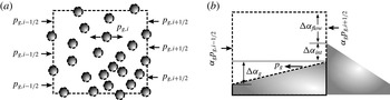
An approach that has been shown to work for coupling compressible gases to compressible liquids with sharp material interfaces is the stratified-flow concept developed by Chang & Liou (Reference Chang and Liou2007). They consider control volumes for the gas and liquid phases separately. In this approach each computational cell edge is divided into gas–gas, liquid–liquid and gas–liquid sections. The hyperbolic fluxes in each section are computed independently with an appropriate Riemann solver. The flux divergence and pressure gradient terms are assembled from the solution all of these Riemann problems. The application of this concept to granular multiphase flows is illustrated in figure 2.
Application of the stratified-flow concept to granular multiphase flows in a control volume used to sum the pressure forces. The computational cell index is
 $i$
and the right and left edges are denoted by
 $i\pm 1/2$
, respectively. (a) Actual control volume. (b) Control volume with particles collapsed.

The stratified-flow concept can be simplified substantially for a granular flow by using the incompressibility assumption of the particles. The volume fraction (while integrating the hyperbolic terms) is controlled by motion of the incompressible particles. This implies that the volume fraction is not a function of the gas-phase state. Thus, the product rule can be applied to the pressure gradient term (
 $\boldsymbol{{\rm\nabla}}{\it\alpha}_{g}p_{g}$
), which simplifies the gas-phase momentum equation to
 $$\begin{eqnarray}\frac{\partial {\it\alpha}_{g}{\it\rho}_{g}\boldsymbol{v}_{g}}{\partial t}+\boldsymbol{{\rm\nabla}}\boldsymbol{\cdot }({\it\alpha}_{g}{\it\rho}_{g}\boldsymbol{v}_{g}\boldsymbol{v}_{g})=-{\it\alpha}_{g}\boldsymbol{{\rm\nabla}}p_{g}+\boldsymbol{f}_{Lift}+{\it\alpha}_{g}{\it\rho}_{g}\boldsymbol{g}.\end{eqnarray}$$
It is straightforward to satisfy the pressure non-disturbing condition with this simplification because there is only one pressure term to compute rather than having to perfectly balance two separate pressure terms.
This simplification used to produce (4.10) is only rigorously possible to make if the particles are assumed to be incompressible. If the particles are compressible, the solid material density would be a function of
 $T_{s}$
and the total isotropic stress acting on the particle (i.e.
 ${\it\rho}_{s}={\it\rho}_{s}(T_{s},p_{g},p_{s,tot})$
). Conservation of particle mass would then dictate that the solid volume fraction is implicitly a function of
 ${\it\rho}_{s}$
, since
 ${\it\alpha}_{s}{\it\rho}_{s}$
is a conserved variable. For example, the high pressure behind a gas-phase shock would increase
 ${\it\rho}_{s}$
, with a resulting decrease in particle diameter, and, in turn, decrease
 ${\it\alpha}_{s}$
. Thus, a gas-phase shock would cause a discontinuous decrease of
 ${\it\alpha}_{s}$
in addition to a pressure jump. As a result, the quantity
 ${\it\alpha}_{g}p_{g}$
is, in general, non-differentiable and
 $\boldsymbol{{\rm\nabla}}{\it\alpha}_{g}p_{g}\neq {\it\alpha}_{g}\boldsymbol{{\rm\nabla}}p_{g}+p_{g}\boldsymbol{{\rm\nabla}}{\it\alpha}_{g}$
across a shock. However, if particle incompressibility is assumed, then
 ${\it\rho}_{s}={\it\rho}_{s}(T_{s})$
and
 $\boldsymbol{{\rm\nabla}}{\it\alpha}_{g}p_{g}={\it\alpha}_{g}\boldsymbol{{\rm\nabla}}p_{g}+p_{g}\boldsymbol{{\rm\nabla}}{\it\alpha}_{g}$
, since
 ${\it\alpha}_{s}$
would then not be an implicit function of the gas-phase pressure and, as a result, would not change discontinuously due to compression behind a gas-phase shock.
One issue that merging the pressure gradient and nozzling terms introduces in (4.10) is that there are no portions of the gas-phase hyperbolic terms that resemble the Euler equations. As a result, standard Godunov methods cannot be used. Despite this, the control volume shown in figure 2 is still valid and the solution to the Riemann problem on the gas–gas fraction of the cell face where gas flows between the particles is physically correct. We use this observation and solve a gas-phase Riemann problem at the section marked
 ${\rm\Delta}{\it\alpha}_{flow}$
in figure 2. The pressure computed from this Riemann problem (
 $p_{g,i+1/2}$
) is stored at each cell edge and used to compute the non-conservative pressure term
 ${\it\alpha}_{g}\boldsymbol{{\rm\nabla}}p_{g}$
at each computational cell edge. This is computed in the
 $x$
-direction by
 $$\begin{eqnarray}{\it\alpha}_{g}\frac{\partial p_{g}}{\partial x}\approx {\it\alpha}_{g,i}\frac{p_{g,i+1/2}-p_{g,i-1/2}}{{\rm\Delta}x},\end{eqnarray}$$
where
 ${\rm\Delta}x$
is the width of a computational cell.
The only requirement for evaluating the gas-phase Riemann problem is that pressure is explicitly calculated and is not directly included in the momentum flux. The HLLC (Harten, Lax & van Leer Reference Harten, Lax and van Leer1983; Toro, Spruce & Speares Reference Toro, Spruce and Speares1994) and AUSM (Liou Reference Liou2006) flux schemes can be modified to match this condition. The HLLC flux is used in this work (see appendix B.2). The remaining flux derivatives are computed in a similar manner. For example, the enthalpy flux divergence is
 $$\begin{eqnarray}\frac{\partial {\it\alpha}_{g}{\it\rho}_{g}u_{g}H_{g}}{\partial x}\approx \frac{{\it\alpha}_{g,i+1/2}{\it\rho}_{g,i+1/2}u_{g,i+1/2}H_{g,i+1/2}-{\it\alpha}_{g,i-1/2}{\it\rho}_{g,i-1/2}u_{g,i-1/2}H_{g,i-1/2}}{{\rm\Delta}x},\end{eqnarray}$$
where
 ${\it\rho}_{g,i+1/2}$
,
 $u_{g,i+1/2}$
and
 $H_{g,i+1/2}$
come from the HLLC Riemann solver and
 ${\it\alpha}_{g,i+1/2}$
is computed using the flux scheme for the granular phase discussed below. More details of the gas-phase solution for the hyperbolic terms can be found in appendix B.
4.1.2. Granular fluxes
Calculation of the granular flux has its own particular set of complications. One issue is its extreme stiffness as the packing limit is approached and the friction pressure and the compaction wave speed increase towards infinity. In such regions, any minute fluctuation of solid volume fraction can produce extremely large changes in friction pressure. The solution we are using to avoid numerical instability is to smoothly degrade the order of the numerical method from fifth-order to first-order as the packing limit is approached. This helps to maintain numerical stability and monotonic solutions of the granular conservative variables. The details of this process are discussed in appendix B.4.
One of the most difficult issues is that the compaction wave speed and solid pressure become zero (1) when the granular temperature is zero or (2) at low volume fractions, resulting in hyperbolic degeneracy (as discussed previously). One approximate Riemann solver used for the particulate phase for a pressureless (
 $p_{s,tot}=0$
) dust model is from Collins et al. (Reference Collins, Ferguson, Chien, Kuhl, Krispin and Glaz1994):
 $$\begin{eqnarray}\boldsymbol{F}_{s,i+1/2}=\left\{\begin{array}{@{}ll@{}}\boldsymbol{F}_{s}(\boldsymbol{U}_{s}^{L})\quad & \text{if }u_{s}^{L}\geqslant 0\text{ and }u_{s}^{R}>0,\\ \boldsymbol{F}_{s}(\boldsymbol{U}_{s}^{R})\quad & \text{if }u_{s}^{L}<0\text{ and }u_{s}^{R}\leqslant 0,\\ \boldsymbol{F}_{s}(\boldsymbol{U}_{s}^{L})+\boldsymbol{F}_{s}(\boldsymbol{U}_{s}^{R})\quad & \text{if }u_{s}^{L}>0\text{ and }u_{s}^{R}<0,\\ 0\quad & \text{if }u_{s}^{L}<0\text{ and }u_{s}^{R}>0,\end{array}\right.\end{eqnarray}$$
where
 $\boldsymbol{U}_{s}^{L,R}$
are the left- and right-reconstructed conserved variable vector for the solid phase at edge
 $i+1/2$
and
 $\boldsymbol{F}_{s}$
is the flux vector of the particle phase, excluding solids pressure and the non-conservative terms. In other locations, where the granular phase is not pressureless, (4.13) is incorrect and a more usual Riemann solver will work. Ideally, however, the same Riemann solver would handle both cases without any ad hoc switches, which is the case for the AUSM
 $^{+}$
-up solver (Liou Reference Liou2006). In addition to reducing the order of the numerical method to first order in highly packed regions, an additional dissipative term is added to the AUSM flux for the granular phase. Numerical details of the modified AUSM flux for the granular phase are given in § B.4.
 $\text{AUSM}^{+}$
-up is also modified to return
 $u_{s,i+1/2}$
needed for
 $p_{s}\boldsymbol{{\rm\nabla}}\boldsymbol{\cdot }\boldsymbol{v}_{s}$
, the quantity
 ${\it\alpha}_{s,i+1/2}u_{s,i+1/2}$
for the
 $pDV$
work term (
 $p_{g}\boldsymbol{{\rm\nabla}}\boldsymbol{\cdot }{\it\alpha}_{s}\boldsymbol{v}_{s}$
), and
 ${\it\alpha}_{g,i+1/2}$
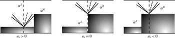
needed to complete the gas-phase fluxes. Computation of the gas-phase edge volume fraction is based on where the particles have moved at
 $t=0^{+}$
, as shown in figure 3, and the gas-phase volume fraction at the cell edge is computed by
 $$\begin{eqnarray}{\it\alpha}_{g,i+1/2}=\left\{\begin{array}{@{}ll@{}}{\it\alpha}_{g,i+1/2}^{L}\quad & \text{if }{\dot{m}}_{s,i+1/2}>0,\\ {\it\alpha}_{g,i+1/2}^{R}\quad & \text{if }{\dot{m}}_{s,i+1/2}\leqslant 0,\end{array}\right.\end{eqnarray}$$
where
 ${\dot{m}}_{s,i+1/2}$
is the granular mass flux calculated from the AUSM
 $^{+}$
-up flux (see § B.4 for details). Similarly,
 $$\begin{eqnarray}\displaystyle & \displaystyle {\it\alpha}_{s,i+1/2}u_{s,i+1/2}=\left\{\begin{array}{@{}ll@{}}{\dot{m}}_{s,i+1/2}/{\it\rho}_{s,i+1/2}^{L}\quad & \text{if }{\dot{m}}_{s,i+1/2}>0,\\ {\dot{m}}_{s,i+1/2}/{\it\rho}_{s,i+1/2}^{R}\quad & \text{if }{\dot{m}}_{s,i+1/2}\leqslant 0,\end{array}\right. & \displaystyle\end{eqnarray}$$
 $$\begin{eqnarray}\displaystyle & \displaystyle u_{s,i+1/2}=\left\{\begin{array}{@{}ll@{}}{\dot{m}}_{s,i+1/2}/{\it\alpha}_{s,i+1/2}^{L}{\it\rho}_{s,i+1/2}^{L}\quad & \text{if }{\dot{m}}_{s,i+1/2}>0,\\ {\dot{m}}_{s,i+1/2}/{\it\alpha}_{s,i+1/2}^{R}{\it\rho}_{s,i+1/2}^{R}\quad & \text{if }{\dot{m}}_{s,i+1/2}\leqslant 0.\end{array}\right. & \displaystyle\end{eqnarray}$$
 $$\begin{eqnarray}p_{s}\frac{\partial u_{s}}{\partial x}\approx p_{s,i}\frac{u_{s,i+1/2}-u_{s,i-1/2}}{{\rm\Delta}x},\end{eqnarray}$$
and the
 $pDV$
term can be approximated as
 $$\begin{eqnarray}p_{g}\frac{\partial {\it\alpha}_{s}u_{s}}{\partial x}\approx p_{g,i}\frac{{\it\alpha}_{s,i+1/2}u_{s,i+1/2}-{\it\alpha}_{s,i-1/2}u_{s,i-1/2}}{{\rm\Delta}x}.\end{eqnarray}$$
Schematic of the gas-phase volume fraction at a cell face at
 $t=0^{+}$
.

5. Verification test problems
A series of one-dimensional numerical experiments were performed to assess the accuracy and robustness of the method. The solutions were advanced in time using a third-order Runge–Kutta (Spiteri & Ruuth Reference Spiteri and Ruuth2003) algorithm with a Courant–Friedrichs–Lewy (CFL) number of 0.5, based on the maximum wave speed,
 ${\it\lambda}_{max}=\max (|u_{g}|+c_{g},|u_{s}|+c_{s})$
. Solid volume fractions below
 $10^{-10}$
are set to zero. Boundary conditions for the granular phase were either reflected for a symmetry condition or extrapolated for inflow and outflow. The coefficient of restitution for the granular phase is
 $e=0.999$
unless specified otherwise. The parameters
 ${\it\alpha}_{s,crit}$
and
 ${\it\alpha}_{s,max}$
were 0.5 and 0.65, respectively. The granular dissipation parameter is
 $\mathscr{D}=1$
(see § B.4) unless stated otherwise. Multidimensional tests employ block-structured adaptive mesh refinement (AMR) with the PARAMESH library (MacNeice et al.
Reference MacNeice, Olson, Mobarry, de Fainchtein and Packer2000). Refinement is based on smoothness of the mixture density
 ${\it\rho}_{m}={\it\alpha}_{g}{\it\rho}_{g}+{\it\alpha}_{s}{\it\rho}_{g}$
. Details of how PARAMESH was used for this work can be found in Houim & Kuo (Reference Houim and Kuo2011). Adaptive mesh refinement was not used for one-dimensional test problems.
5.1. Advection of a particle curtain
Here we examine the ability of the model and numerical algorithm to preserve the pressure non-disturbing condition near a steep granular interface. We advect a curtain of particles with a volume fraction of 40 % in a domain with uniform velocity, pressure and temperature of
 $100~\text{m}~\text{s}^{-1}$
, 1 atm and 300 K, respectively. To increase the complexity of the calculation, we also place a bubble of pure helium where the particles are located. The gas surrounding the He bubble is pure nitrogen. Specifically, the initial conditions are:
 $Y_{\text{N}_{2}}=1$
and
 ${\it\alpha}_{s}=0.4$
if
 $0.4<x<0.6$
and
 $Y_{\text{He}}=1$
and
 ${\it\alpha}_{s}=0$
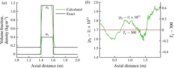
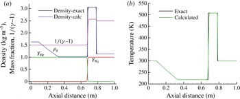
otherwise. The domain was discretized with 200 grid points per metre. Inflow and outflow boundary conditions were used on the left and right boundaries, respectively. We advect the combined granular and gaseous material interface. The particle and helium curtain should be passively advected downstream without changing the pressure and temperature fields. The computed solution, shown in figure 4, indicates that temperature and pressure error are negligible and that the pressure non-disturbing condition is met.
Advection of a granular and multicomponent gaseous interface with uniform temperature for a distance of 1 m. (a) Comparison of gas-phase density and
 ${\it\alpha}_{s}$
to the exact solution and (b) gas-phase temperature and error in pressure.

5.2. Two-phase granular shock-tube problem
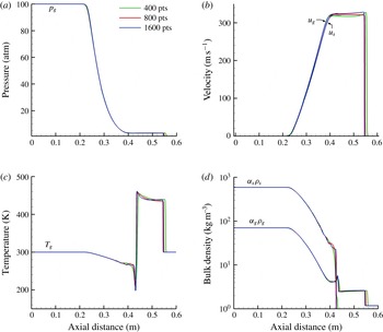
In this section we test the ability of the model and solution procedure to solve shock-tube problems with low particle volume fraction. The granular-phase solids and frictional–collisional pressures are nearly zero due to the low particle volume fraction. As discussed above, this creates hyperbolically degenerate conditions that are difficult for most standard Riemann solvers to deal with. It is a situation that we must test to ensure that the computed results agree with reference calculations that used specialized Riemann solvers developed for pressureless dust. The initial conditions follow (Saito et al. Reference Saito, Marumoto and Takayama2003; Fedorov et al. Reference Fedorov, Kharlamova and Khmel’2007):
 $$\begin{eqnarray}\left.\begin{array}{@{}c@{}}p_{g}^{L}=10~\text{atm},\quad p_{g}^{R}=1~\text{atm},\\ T^{L}=270~\text{K},\quad T^{R}=270~\text{K},\\ Y_{g,air}^{L}=1,\quad Y_{g,air}^{R}=1,\\ {\it\alpha}_{s}^{L}=0,\quad {\it\alpha}_{s}^{R}=5.172\times 10^{-4},\\ {\it\Theta}_{s}^{L}=0,\quad {\it\Theta}_{s}^{R}=0.\end{array}\right\}\end{eqnarray}$$
The density, diameter and specific heat of the particles are
 ${\it\rho}_{s}=2500~\text{kg}~\text{m}^{-3}$
,
 $d_{s}=10~{\rm\mu}\text{m}$
and
 $C_{V,s}=718~\text{J}~\text{kg}^{-1}~\text{K}^{-1}$
, respectively. The domain is
 $0.257798$
m in length and the diaphragm is placed at
 $0.129$
m. The solution at
 $184~{\rm\mu}$
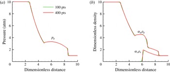
s after the diaphragm is ruptured is shown in figure 5 for two grid spacings. The physics of dust–gas shock-tube problems are well known (Miura & Glass Reference Miura and Glass1982; Saito et al.
Reference Saito, Marumoto and Takayama2003); nevertheless, there are no exact solutions that can be used for verification. Instead, the computed results can be compared with reference solutions from Saito et al. (Reference Saito, Marumoto and Takayama2003) and Fedorov et al. (Reference Fedorov, Kharlamova and Khmel’2007). The results, shown in figure 5, compare well with computed results from these references, which indicates that our modified AUSM
 $^{+}$
-up scheme used to compute the granular flux (see § B.4) is accurate when the dust is nearly pressureless.
Computed (a) gas-phase pressure and (b) bulk densities for the gas and granular phases for the two-phase granular Riemann problem at
 $184~{\rm\mu}\text{s}$
. The densities were scaled by the initial gas-phase density to the right of the interface. The length scale was scaled so that the domain ranges from 0 to 10 to match the output used by Fedorov et al. (Reference Fedorov, Kharlamova and Khmel’2007).

The burst of the diaphragm sends a shock wave into the low-pressure air and particle mixture, a rarefaction wave into the high-pressure side, and a gas-phase contact surface that passes through the particles. Drag forces between the post-shock gas and particles locally decelerate the gas and produce a subsequent rise in pressure. The pressure increase is due to high-speed gas from regions without particles flowing into and filling a region where gas has been decelerated by drag. The local increase in pressure produces acoustic waves that propagate towards the rarefaction and cause the hook-like structure at
 $x\sim 5$
. Mechanical and thermal losses of the post-shock gases due to drag also have the effect of weakening the shock, which is illustrated in the next test problem. The two-phase shock wave formed in this test problem corresponds to a Type I structure characterized by Khmel’ & Fedorov (Reference Khmel’ and Fedorov2014
a
,Reference Khmel’ and Fedorov
b
), where there is a discontinuous gas-phase shock that propagates through the particles with smooth relaxation of granular properties, such as volume fraction, behind the shock.
5.3. Two-phase granular shock-tube problem with a gaseous He–
$N_{2}$
interface

This problem is similar to the test presented in the previous section, but now we add a gaseous material interface. This examines whether the model and numerical method can produce the correct weak solution for a multiphase shock-tube problem that contains a gaseous material interface with varying
 ${\it\gamma}$
. Such a situation may exist in a dust explosion when shocks interact with thin dust flames that can separate reactants and products, which have different specific heat ratios. Here the high-pressure side contains pure helium and the low-pressure side contains a mixture of particles and pure N
 $_{2}$
. The initial states for this test case are
 $$\begin{eqnarray}\left.\begin{array}{@{}c@{}}p_{g}^{L}=10~\text{atm},\quad p_{g}^{R}=1~\text{atm},\\ T^{L}=300~\text{K},\quad T^{R}=300~\text{K},\\ Y_{g,\text{He}}^{L}=1,\quad Y_{g,\text{He}}^{R}=0,\\ Y_{g,\text{N}_{2}}^{L}=0,\quad Y_{g,\text{N}_{2}}^{R}=1,\\ {\it\alpha}_{s}^{L}=0,\quad {\it\alpha}_{s}^{R}=4.555\times 10^{-4},\\ {\it\Theta}_{s}^{L}=0,\quad {\it\Theta}_{s}^{R}=0.\end{array}\right\}\end{eqnarray}$$
The density, specific heat and restitution coefficient of the particles are
 $2500~\text{kg}~\text{m}^{-3}$
,
 $745~\text{J}~\text{kg}^{-1}~\text{K}^{-1}$
and
 $0.999$
, respectively. The domain is
 $1$
m in length and the diaphragm is placed at
 $0.5$
m. The volume fraction of the right state was chosen so that the bulk densities of the gas and granular phases were the same. Calculations were done for two different particle diameters, 10 and
 $25~{\rm\mu}\text{m}$
. The equations were integrated up to
 $400~{\rm\mu}\text{s}$
of physical time and 400 grid points were used in each calculation. A comparison of the computed results to the exact solution for this Riemann problem when particles are not present is shown in § B.2.
The results, shown in figure 6, are qualitatively similar to the previous test problem. The gas-phase pressure in multiphase shock tubes is actually higher if particles are present, even though the shock is weaker (smaller pressure jump and lower speed). Both of these are side effects of mechanical losses to the post-shock gas from drag as discussed earlier. The locally higher value of the solid bulk density and velocity at
 ${\sim}0.65$
m is caused by a sharp change in the drag force at the He–
 $\text{N}_{2}$
contact surface. This causes a pile-up of particles on the nitrogen side of the gas-phase contact surface where the drag force is higher. The solids pressure is very small and has a negligible influence for the low volume fractions in this problem. Spurious oscillations are not present near the granular or He–
 $\text{N}_{2}$
contact surfaces, which indicates that the model and solution method can accurately solve two-phase granular shock-tube problems that contain mixtures of gases with varying specific heats.
Computed (a) gas-phase and solids pressure, (b) velocity, (c) temperature and (d) bulk density for multiphase shock-tube problem with a He–
 $\text{N}_{2}$
interface at
 $400~{\rm\mu}\text{s}$
. The solid temperature and velocity are not shown if the particle volume fraction lies below
 $10^{-8}$
.

5.4. Dense granular two-phase shock-tube problem
The solids and frictional–collisional pressures were negligible in the previous problems. This test is for a two-phase shock-tube problem with a high driving pressure of 100 atm and a dense particle volume fraction of 40 %. This situation tests whether the model can predict relaxation structures of granular shocks (Kamenetsky et al. Reference Kamenetsky, Goldshtein, Shapiro and Degani2000). This case also stresses capabilities of the solution method to compute high-pressure gases interacting with dense granular regions that approach the packing limit with steep granular interfaces. The initial states for this problem are
 $$\begin{eqnarray}\left.\begin{array}{@{}c@{}}p_{g}^{L}=100~\text{atm},\quad p_{g}^{R}=1~\text{atm},\\ T^{L}=300~\text{K},\quad T^{R}=300~\text{K},\\ Y_{g,Air}^{L}=1,\quad Y_{g,Air}^{R}=1,\\ {\it\alpha}_{s}^{L}=0,\quad {\it\alpha}_{s}^{R}=0.4,\\ {\it\Theta}_{s}^{L}=0,\quad {\it\Theta}_{s}^{R}=0.\end{array}\right\}\end{eqnarray}$$
The domain measures 0.06 m in length and the diaphragm is placed at 0.03 m. The resulting shock structure is advanced for 100
 ${\rm\mu}\text{s}$
on a grid with 1200 computational cells. The particle diameter, density, specific heat and coefficient of restitution were
 $5~{\rm\mu}\text{m}$
,
 $1470~\text{kg}~\text{m}^{-3}$
,
 $987~\text{J}~\text{kg}^{-1}~\text{K}^{-1}$
and 0.999, respectively. The volume fraction in this problem approaches the packing limit and additional dissipation was added to the granular phase by setting the hyperbolic dissipation parameter (
 $\mathscr{D}$
) to 1 (see (B 25) in § B.4). The solution at
 $100~{\rm\mu}\text{s}$
is shown in figure 7. The influence of
 $\mathscr{D}$
and coefficient of restitution (e) on the granular shock structure are shown in figures 8 and 9.
Computed (a) pressure, (b) velocity, (c) temperature and (d) bulk density for the dense granular shock-tube problem at
 $100~{\rm\mu}\text{s}$
with
 $e=0.999$
and
 $\mathscr{D}=1$
.

Effect of
 $\mathscr{D}$
and
 $e$
on calculated profiles of
 ${\it\alpha}_{s}$
and
 ${\it\Theta}_{s}$
near a granular shock: (a)
 $e=0.999$
, (b)
 $e=0.9$
.

Effect of
 $\mathscr{D}$
and
 $e$
on calculated profiles of pressure and
 $p_{fric}/p_{s,tot}$
near a granular shock: (a)
 $e=0.999$
, (b)
 $e=0.9$
.

Unlike previous problems shown in §§ 5.1–5.3, particle–particle interactions are now dominant. After the diaphragm is ruptured, a strong granular shock is transmitted into the granular phase due to the combination of Archimedes forces (
 ${\it\alpha}_{s}\boldsymbol{{\rm\nabla}}p_{g}$
) and particle drag from the high-pressure gas flowing into the dense layer of particles. Frictional heating from gas initially penetrating the particle bed increases the gas and particle temperature by
 ${\sim}2.5$
K near the contact surface. The computed granular shock has a relaxation structure similar to those reported by Kamenetsky et al. (Reference Kamenetsky, Goldshtein, Shapiro and Degani2000). Sources of granular energy,
 $E_{s}$
, decrease rapidly away from the granular shock. Without these sources, collisional dissipation of
 $E_{s}$
(
 $\dot{{\it\gamma}}$
) decreases
 ${\it\Theta}_{s}$
and
 $p_{s}$
. Nevertheless, mechanical equilibrium needs to be maintained and the solid volume fraction rises to compensate for the reduction in
 ${\it\Theta}_{s}$
by packing even further to increase the friction pressure. Eventually, the granular temperature decreases to zero, and the total intergranular stress,
 $p_{s,tot}$
, is solely from friction pressure, as shown in figure 9. The granular temperature decreases much faster and the resulting granular shock structure is almost entirely due to friction pressure when the coefficient of restitution is lowered to 0.9.
A weak gas-phase shock-like structure is present at the location of the granular shock. This is due to the increase in particle volume fraction, which compresses the gas and produces a sharp rise in temperature and pressure along with the propagating granular shock. This corresponds to a Type II two-phase granular shock structure characterized by Khmel’ & Fedorov (Reference Khmel’ and Fedorov2014
a
,Reference Khmel’ and Fedorov
b
), a case where a propagating granular shock drives a weak propagating gas-phase discontinuity along with it. This structure is in contrast to the Type I structure mentioned above, where a gas-phase shock drives a smooth compression of particles (increase of
 ${\it\alpha}_{s}$
).
A peculiarity of granular systems is that shocks form in granular systems even though
 $c_{s}$
and
 $p_{s,tot}$
can be zero in front of the shock. Assuming that the intergranular stress and particle velocity are zero upstream of the shock and
 $p_{s,tot}=p_{fric}$
, it can be shown through a Rankine–Hugoniot analysis that the shock and post-shock particle velocities for a purely granular system are
 $$\begin{eqnarray}u_{shock}=\sqrt{\frac{{\it\alpha}_{s,2}}{{\it\alpha}_{s,2}-{\it\alpha}_{s,1}}\frac{p_{fric}({\it\alpha}_{s,2})}{{\it\alpha}_{s,1}{\it\rho}_{s}}},\quad u_{s,2}=\sqrt{\frac{{\it\alpha}_{s,2}-{\it\alpha}_{s,1}}{{\it\alpha}_{s,2}}\frac{p_{fric}({\it\alpha}_{s,2})}{{\it\alpha}_{s,1}{\it\rho}_{s}}},\end{eqnarray}$$
where states 1 and 2 refer to conditions upstream and downstream of the shock, respectively. Applying the post-shock volume fraction shown in figure 8(b) (
 ${\it\alpha}_{s,2}=0.639$
and
 ${\it\alpha}_{s,1}=0.4$
) produces a shock velocity of
 $186~\text{m}~\text{s}^{-1}$
(corresponding to a position of 0.0486 m after
 $100~{\rm\mu}\text{s}$
) and a particle velocity of
 $69.7~\text{m}~\text{s}^{-1}$
. These analytical values are close enough to the computed results shown in figures 7(b) and 9(b), considering that the gas phase was not taken into account when computing the analytical post-shock condition.
Small gas-phase temperature oscillations of the order of 1 K are present near the granular shock. These do not cause any numerical instabilities and quickly damp from heat transfer between the gas and granular phases. The bump in gas-phase velocity near the solid contact surface in figure 7 is caused by a reduction in flow area when the gas flows into the particles. Oscillations of pressure, velocity and temperature near the granular interface are not present.
The effectiveness of increasing
 $\mathscr{D}$
to control oscillations of intergranular stress in dense granular regions is shown in figure 9(b). Severe oscillations of friction pressure are produced when
 $\mathscr{D}$
is zero, but increasing it to 1 or 10 effectively eliminates the oscillations at the cost of some numerical diffusion of granular interfaces.
5.5. High-pressure outgassing
The previous problem simulated high-pressure gas entering a region of dense particles. The next problem, on the other hand, simulates high-pressure gas leaving a region of dense particles. Consider high-pressure gas that has been injected into a granular layer as a shock passes over. This gas will be ejected when a subsequent expansion wave reduces the pressure at the surface. The outflow induced by the expansion wave will entrain some of the particles. The same initial conditions as the previous problem are used, with the exception that the particles are now located in the high-pressure region of the shock tube,
 $$\begin{eqnarray}\left.\begin{array}{@{}c@{}}p_{g}^{L}=100~\text{atm},\quad p_{g}^{R}=1~\text{atm},\\ T^{L}=300~\text{K},\quad T^{R}=300~\text{K},\\ Y_{g,Air}^{L}=1,\quad Y_{g,\mathit{Air}}^{R}=1,\\ {\it\alpha}_{s}^{L}=0.4,\quad {\it\alpha}_{s}^{R}=0.0,\\ {\it\Theta}_{s}^{L}=0,\quad {\it\Theta}_{s}^{R}=0.\end{array}\right\}\end{eqnarray}$$
The domain is 0.6 m long and the diaphragm was placed at 0.3 m. The solution at
 $400~{\rm\mu}\text{s}$
is shown in figure 10 for three grid resolutions.
A right-running shock wave and left-running rarefaction wave are produced, similar to the other shock-tube problems. Now, however, drag and buoyancy forces are induced by the escaping gas from the granular bed, and this ejects particles. This process reduces the particle volume fraction to a profile that is similar in form to the gaseous rarefaction wave. Intense mechanical and thermal losses to the gas phase by entraining particles severely weaken the transmitted gaseous shock. The spikes in temperature near the granular interface are physical and result from particles heating the gas at the gas-phase contact surface and a slight gap between the gas and granular contact surfaces (see figure 10 d). If the particles were not present, the temperature would be much higher in the post-shock state and much lower behind the gas-phase contact surface.
Computed (a) gas-phase pressure, (b) velocity, (c) gas-phase temperature and (d) bulk density for high-pressure gaseous ejection from a dense layer of particles at a time of
 $400~{\rm\mu}\text{s}$
. The solid velocity is not shown if the particle volume fraction lies below
 $10^{-8}$
.

5.6. Interaction of a shock wave with a low-volume-fraction dust layer
This problem models the interaction of a shock wave with a loose dust layer. A schematic diagram of the geometrical set-up and initial and boundary conditions is shown in figure 11. The heights of the channel and dust layer are 6 cm and 2 cm, respectively. The left edge of the dust pile is placed at 2 cm, and the shock is initially located at 1 cm. A shock of Mach number 1.6 propagates into air at 1 atm and 288 K. The initial volume fraction of the dust layer is 0.04 %. The particle diameter, density and specific heat are
 $d_{s}=5~{\rm\mu}\text{m}$
,
 ${\it\rho}_{s}=1470~\text{kg}~\text{m}^{-3}$
and
 $C_{V,s}=987~\text{J}~\text{kg}^{-1}~\text{K}^{-1}$
, respectively. Figure 12 shows the computed mixture density at
 $900~{\rm\mu}\text{s}$
for grid spacings of 1.67, 0.83 and 0.42 mm at the finest AMR refinement level. The computed solutions, including the particle and gas-phase vortices, converge with increasing grid resolution.
Schematic diagram of the initial conditions used for multidimensional test problems.

Computed mixture density (
 ${\it\rho}_{m}={\it\alpha}_{g}{\it\rho}_{g}+{\it\alpha}_{s}{\it\rho}_{s}$
, in units of
 $\text{kg}~\text{m}^{-3}$
) for the low-volume-fraction shock wave and dust layer interaction problem at
 $900~{\rm\mu}\text{s}$
for three different grids: (a)
 ${\rm\Delta}x_{min}=1.67$
mm, (b) 0.83 mm and (c) 0.42 mm.

Figure 12 shows that a vortex is introduced in the gas phase from a shear layer produced as particle drag locally decreases the fluid velocity in the granular layer. The gas-phase vortex entrains some of the particles. The particle vortex does not exactly coincide with the gas-phase vortex due to particle inertia. Mechanical and thermal losses from entraining particles cause the shock near the top of the layer to curve and weaken with time. Drag from high-pressure gas entering the layer from the
 $y$
-direction compresses the particles, which thins the dust layer immediately behind the shock. These results agree well with those of Fedorov & Fedorchenko (Reference Fedorov and Fedorchenko2010), in spite of the use of different drag and convective heat transfer models.
6. Experimental validation
The previous tests examined various aspects of the solver and made comparisons to accepted numerical or exact solutions. In this section we compare computed results to experimental measurements. Two geometric configurations are considered. The first configuration is a shock wave interacting with a particle curtain (Rogue et al. Reference Rogue, Rodriguez, Haas and Saurel1998; Ling et al. Reference Ling, Wagner, Beresh, Kearney and Balachandar2012). Here the position of the particle fronts and shock-wave locations are compared to experimental measurements. The second configuration is a shock wave interacting with a layer of dust, where the transmission angles of an oblique transmitted granular shock and granular contact surface are compared to experimental measurements made by Fan et al. (Reference Fan, Chen, Jiang and Li2007). An additional test, not presented in this paper, which uses the same model and solution algorithm, is one in which the high-speed flow behind a shock lifts and entrains dust from a dense layer (Houim & Oran Reference Houim and Oran2015 a ).
6.1. Shock and particle-curtain interaction
Here we test the model against nearly one-dimensional multiphase shock-tube experimental measurements in which a shock wave interacts with a curtain of particles. Two conditions are tested: a lower-volume-fraction particle curtain (Wagner et al.
Reference Wagner, Beresh, Kearney, Trott, Castaneda, Pruett and Baer2012) and a high-volume-fraction particle curtain (Rogue et al.
Reference Rogue, Rodriguez, Haas and Saurel1998). A schematic diagram of the initial conditions and qualitative
 $x$
–
 $t$
diagram of the wave structures produced from a shock interacting with a particle curtain are shown in figure 13. A shock travelling at velocity
 $u_{sh}$
and strength
 $M_{sh}$
impacts a curtain of particles of length
 $L$
and initial volume fraction
 ${\it\alpha}_{s,0}$
. Drag forces resulting from gases that enter and flow through the particle bed and buoyancy forces (
 ${\it\alpha}_{s}\boldsymbol{{\rm\nabla}}p_{g}$
) from gas pushing on the granular interface accelerate the particles. Gas-phase energy that is not reflected or dissipated to the particles during the acceleration stage is transmitted to the downstream side of the particle bed in the form of a weak shock. The computational domain measured from
 $-100L$
to
 $100L$
is discretized with 4000 computational cells. Non-reflecting conditions were used on the left and right boundaries. The upstream edge of the particle curtain is placed at
 $x=0$
.
Initial conditions and qualitative
 $x{-}t$
diagram for the shock wave interacting with a particle curtain.

6.1.1. Particle curtain with
${\it\alpha}_{s,0}=21\,\%$

Here we compare results of computations to experimental measurements made using the multiphase shock-tube apparatus described in Wagner et al. (Reference Wagner, Beresh, Kearney, Trott, Castaneda, Pruett and Baer2012). Specifically, we simulate case 1 of Ling et al. (Reference Ling, Wagner, Beresh, Kearney and Balachandar2012), which presents additional data and compares the results of a Lagrangian multiphase model to these measurements. The length of the particle curtain is 2 mm. The initial volume fraction, diameter, density and specific heat of the soda lime particles is
 $21\,\%$
,
 $115~{\rm\mu}\text{m}$
,
 $2520~\text{kg}~\text{m}^{-3}$
and
 $840~\text{J}~\text{kg}^{-1}~\text{K}^{-1}$
, respectively. A Mach 1.66 shock propagates into air initially at 82.7 kPa and 296.4 K. Comparisons of the computed results and experimental data are shown in figure 14.
Computed
 $x$
–
 $t$
diagram of (a) gas-phase density (in units of
 $\text{kg}~\text{m}^{-3}$
) and (b) solid volume fraction for Mach 1.66 shock interacting with a particle curtain with
 $L=2$
mm. The particles were
 $115~{\rm\mu}\text{m}$
in diameter and had an initial volume fraction of 21 %. Experimental data presented in Ling et al. (Reference Ling, Wagner, Beresh, Kearney and Balachandar2012) and Wagner et al. (Reference Wagner, Beresh, Kearney, Trott, Castaneda, Pruett and Baer2012) are represented by symbols.

The locations of the reflected shock, the transmitted shock and the upstream and downstream fronts of the particle curtain are in close agreement with experimental data. The largest discrepancy is the location of the upstream front of particles. The magnitude of this error depends on a precise definition of the particle-curtain edge, which is not stated in Ling et al. (Reference Ling, Wagner, Beresh, Kearney and Balachandar2012) or Wagner et al. (Reference Wagner, Beresh, Kearney, Trott, Castaneda, Pruett and Baer2012). The computed position of the upstream edge of particles lags experimental results from
 $x/L=1.5$
to
 $2$
if a threshold of
 ${\it\alpha}_{s}=0.1\,\%$
or 0.01 % is used to define the edge of the particle curtain. On the other hand, the computed position of the upstream particle edge is much closer if a threshold value of
 ${\it\alpha}_{s}=1\,\%$
is used. The computed downstream edge of the particle curtain agrees well with measurements regardless of how the edge of the particle curtain is defined due to the locally high gradient of volume fraction.
6.1.2. Particle curtain with
${\it\alpha}_{s,0}=65\,\%$

The experiment of Rogue et al. (Reference Rogue, Rodriguez, Haas and Saurel1998) has a much larger volume fraction than the previous test (
 ${\it\alpha}_{s,0}=65\,\%$
). The high initial volume fraction is at a common definition of the random close-packing limit (Agrawal et al.
Reference Agrawal, Loezos, Syamlal and Sundaresan2001; Igci et al.
Reference Igci, Andrews, Sundaresan, Pannala and O’Brien2008). As a result, the parameters
 ${\it\alpha}_{s,crit}$
and
 ${\it\alpha}_{s,max}$
were raised to
 $65\,\%$
and
 $70\,\%$
, respectively, to keep the friction and solids pressures from becoming singular (see (3.21)–(3.23)). The length of the particle curtain is
 $2$
cm. The diameter, density and specific heat of the glass beads that were used to make the curtain are 1.5 mm,
 $2600~\text{kg}~\text{m}^{-3}$
and
 $840~\text{J}~\text{kg}^{-1}~\text{K}^{-1}$
, respectively. A Mach 1.3 shock propagates into air at 1 atm and 294.2 K. Comparisons of the computed results and experimental data are shown in figure 15.
Computed
 $x$
–
 $t$
diagram of (a) gas-phase density (in units of
 $\text{kg}~\text{m}^{-3}$
) and (b) solid volume fraction for Mach 1.3 shock interacting with a particle curtain with
 $L=2$
cm. The particles were 1.5 mm in diameter and had an initial volume fraction of 65 %. Experimental data of Rogue et al. (Reference Rogue, Rodriguez, Haas and Saurel1998) are represented by symbols.

The results of this test case are qualitatively similar to the previous case. One notable exception is that the transmitted shock is much weaker. This is primarily due to the much higher mechanical and thermal losses created as the shock propagates through the highly packed glass beads. The calculated results match closely with the experimental measurement of the downstream particle front. The upstream front of the particles does not agree as well. This is due, in part, to the ambiguity of defining the edge of particles in the computation, which is undefined in Rogue et al. (Reference Rogue, Rodriguez, Haas and Saurel1998). The upstream front of particles is smoother than the downstream edge, and, as a result, the modelling error is highly sensitive to how the particle edge is defined. If a threshold volume fraction of 1 % is used (see figure 15 b), the error is quite large and the front barely appears to move. The agreement between the measurements and the computed results is much better if a threshold volume fraction between 7 % and 10 % is used to define the curtain edge. This ambiguity could be avoided if the particle-curtain edges were precisely defined (based, perhaps, on a threshold volume fraction) in experimental measurements, but this is difficult due to, among other issues, uncertainties of extinction coefficients through particle clouds and details of the experimental apparatus.
Comparison between computed and experimental (Rogue et al. Reference Rogue, Rodriguez, Haas and Saurel1998) pressure–time traces for a Mach 1.3 shock interacting with a dense particle curtain.

Rogue et al. (Reference Rogue, Rodriguez, Haas and Saurel1998) also measured the pressure–time (
 $p$
–
 $t$
) traces at physical distances of
 $-11$
cm (
 $x/L=-5.5$
) and 4.3 cm (
 $x/L=2.15$
) with respect to the upstream edge of the particle curtain. A comparison of the computed to the measured pressure–time traces at these locations is shown in figure 16. The calculations closely match the measurements, and also match the timing and strength of the reflected shock, as well as the subsequent pressure decay as the particle curtain (which acts like a porous moving piston) accelerates. The model results also agree with the strength and timing of the transmitted shock.
The computed
 $p$
–
 $t$
traces do not match as well when the particle cloud arrives at
 $x/L=2.15$
and the measured pressure rises rapidly. The sharp pressure rise is produced as the particle bed moves past the measurement location. The
 $p$
–
 $t$
trace is essentially a record of the pressure drop as a function of position in the particle curtain as it moves past the measurement location, which is highly sensitive to the volume fraction and drag, and, to some extent, to the models selected for solids and frictional–collisional pressure. (A detailed comparison of the effect of drag and frictional–collisional pressure models on the structure of the particle curtain is beyond the scope of this paper and can be undertaken as a separate study.)
6.2. Transmitted granular oblique shock and contact angles
In the experiment of Fan et al. (Reference Fan, Chen, Jiang and Li2007), a shock interacts with a dense layer of dust. The angle that a transmitted compaction wave and granular contact surface make with the horizontal when a shock wave passes over the dust layer, as shown in figure 17(a), was measured. An oblique granular shock is transmitted into the dense layer of dust by forces from high-pressure gas behind the shock pushing on the granular interface as well drag from gases penetrating into the layer. These forces compact the layer and induce an oblique granular contact surface in addition to a transmitted granular shock.
The initial conditions follow the diagram in figure 11. For this test, the layer thickness and domain heights are 2 and 10 cm, respectively. The initial position of the shock is 1 cm, and the left edge of the dust layer is at 0 m. The initial volume fraction was 47 %, and the density, diameter, coefficient of restitution and specific heat of the particles were
 ${\it\rho}_{s}=1100~\text{kg}~\text{m}^{-3}$
,
 $d_{s}=15~{\rm\mu}\text{m}$
,
 $e=0.9$
and
 $C_{V,s}=987~\text{J}~\text{kg}^{-1}~\text{K}^{-1}$
, respectively. The velocity of the shock wave, which propagated into air at 1 atm and 300 K, is
 $990~\text{m}~\text{s}^{-1}$
. The bottom boundary was changed to a non-reflecting condition to avoid reflections and increase the measurement distance for the transmitted compaction wave and granular contact angles. The equations were integrated for
 $100~{\rm\mu}\text{s}$
with
 ${\rm\Delta}x=347~{\rm\mu}\text{m}$
at the smallest level of AMR refinement.
The computed solid volume fraction at
 $100~{\rm\mu}\text{s}$
is shown in figure 17(b). The computed transmission angles of the granular contact surface and compaction wave are
 $1.18^{\circ }$
and
 $4.78^{\circ }$
, respectively, which are close to the measured values of
 $1^{\circ }$
–
 $2^{\circ }$
for the contact surface and
 $4^{\circ }$
for the granular shock (Fan et al.
Reference Fan, Chen, Jiang and Li2007).
Angles of the transmitted compaction wave and granular contact from a shock wave propagating across the dust layer: (a) definition of the angles and (b) computed solution at
 $100~{\rm\mu}\text{s}$
and a grid spacing of
 $347~{\rm\mu}\text{m}$
at the finest level of refinement.

7. Interaction of a shock wave with a dense dust pile
The interaction of a strong Mach 3 shock with a square-edge layer of packed dust is solved to demonstrate the capabilities of the model and solution algorithm. This problem contains all of the challenging features illustrated with previous test problems, including dense granular regions that approach the packing limit, very dilute granular regions that are hyperbolically degenerate, and sharp granular interfaces that interact with a high-speed flow laden with shocks. The initial and boundary conditions follow figure 11. The height of the domain is 10 cm and the height of the dust layer is 6.67 mm. The left edge of the dust pile is at 20 cm, the shock is initially placed at 19 cm, and the overall domain length is 50 cm. The shock propagates into air at 1 atm and 300 K. The initial volume fraction of the dust is 47 %, which corresponds to typical volume fractions of settled layers of dust (Edwards & Ford Reference Edwards and Ford1988; Fan et al.
Reference Fan, Chen, Jiang and Li2007). The particle diameter, density and specific heat are
 $d_{s}=5~{\rm\mu}\text{m}$
,
 ${\it\rho}_{s}=1470~\text{kg}~\text{m}^{-3}$
and
 $C_{V,s}=987~\text{J}~\text{kg}^{-1}~\text{K}^{-1}$
, respectively. The grid spacing at the smallest level of refinement is
 ${\rm\Delta}x=173~{\rm\mu}\text{m}$
.
A sequence showing the solid volume fraction and the numerical gas-phase schlieren (
 $|\boldsymbol{{\rm\nabla}}{\it\rho}_{g}|$
) is shown in figure 18. The entire domain is shown in each image. Note that there are no pressure oscillations evident in the numerical schlieren in front of the dust layer. Initially, when the shock interacts with the dust layer, intense drag and buoyancy forces act on the particles. This rapidly slows the gas and produces a strong reflected shock that resembles the interaction between a shock and a forward-facing step. The post-shock gases, flowing up and around the front edge of the dust pile, entrain some of the dust and cause it to roll up, similar to earlier results in figure 12. The combination of lift forces and particle–particle interactions strip some of the particles from the surface of the rolled-up layer. This produces a particle cloud with a volume fraction around 0.05 %. Intense shear at the top of the layer and various shock reflections into the dust layer eventually destabilize the boundary layer as the shock moves downstream. This perturbs the top of the dust pile and produces the Mach lines shown in the numerical schlieren at 0.49 ms. Similar Mach lines are shown in experimental shadowgraphs of Fan et al. (Reference Fan, Chen, Jiang and Li2007). Perturbing the surface of the layer intensifies turbulence and, as a result, throws more particles up into the post-shock gas. By the end of the calculation, the layer of dust is highly distorted as a result of the turbulence.
Computed time sequence of (a,c,e,g,i) solid volume fraction
 $\log _{10}({\it\alpha}_{s})$
and (b,d,f,h,j) numerical schlieren fields
 $|\boldsymbol{{\rm\nabla}}_{g}|$
for a Mach 3 shock interacting with a dense layer of dust.

Starting at
 ${\sim}0.49$
ms, lines of locally higher particle volume fraction, called particle streamers, start to form. At 2 ms, the volume fraction in these structures ranges from 0.5 % to 20 %. Such structures have been observed in experiments and computations. For example, they are seen in incompressible simulations using kinetic-theory-based granular flow models (Agrawal et al.
Reference Agrawal, Loezos, Syamlal and Sundaresan2001; Igci et al.
Reference Igci, Andrews, Sundaresan, Pannala and O’Brien2008), Eulerian–Lagrangian multiphase models that explicitly account for particle collisions (Helland et al.
Reference Helland, Occelli and Tadrist2000), and in riser experiments (Horio & Kuroki Reference Horio and Kuroki1994). These structures result from two effects: the strong nonlinearity in the drag force as a function of volume fraction, and inelastic collisions locally reducing the solids pressure. Both of these effects produce dense clumps of particles that tend to move as a group and can be around 10 particle diameters in width (Agrawal et al.
Reference Agrawal, Loezos, Syamlal and Sundaresan2001).
8. Summary and conclusions
In this paper, we have presented a granular multiphase model suitable for high-speed flows that can be laden with shocks and contain particle concentrations ranging from dilute to nearly packed. The model resembles some of the granular multiphase models used for incompressible flows (Syamlal et al. Reference Syamlal, Rogers and O’Brien1993; Gidaspow Reference Gidaspow1994), but here it is extended to fully compressible flows. Two sets of Euler equations are coupled, one for the gas phase and another for the granular phase. Intergranular stress representing collisional and friction effects is described through the solids and frictional–collisional pressures. The phases can be coupled by drag, convective heat transfer, phase change, etc. Nevertheless, many physical assumptions, discussed in §§ 3 and 4, were made to justify this form when the flow speed is high and it is compressible. Extending the model to include the granular viscosity terms in the gas- and liquid-like regimes is a topic of ongoing work.
The largest limitation to the model is that it is not valid in the solid-like regions of granular flow, which could be important for simulating phenomena with deep piles of granular material such as dunes. Another limitation is the inability to predict accurately the behaviour of cohesive granular materials, such as powders made of very small particles or wet sand. Overcoming these limitations would necessitate adding granular viscous stresses that resemble plastic flow (Jop, Forterre & Pouliquen Reference Jop, Forterre and Pouliquen2006; Zèmerli Reference Zèmerli2013), stress relaxation models (Zhang Reference Zhang2005), or even Hooke’s law (Andreotti et al. Reference Andreotti, Forterre and Pouliquen2013). Development of stress models for the solid-like regime for pure granular materials (no interstitial fluid between the grains) is an active research area.
There is great uncertainty in the drag and convective heat transfer correlations in high-speed and densely packed regions. We found that the drag correlation of Gidaspow (Reference Gidaspow1994) works surprisingly well, given that it was developed for low-speed flows. Arguably, drag models for compressible flow (Parmar et al. Reference Parmar, Haselbacher and Balachandar2010) would be better in low-volume-fraction regions, but have not been extended to dense regions. The Ergun equation (the limit of (3.37) at high particle volume fraction) is probably more appropriate in dense regions that resemble a fluidized bed, but has not been extended to compressible flows. Similar problems exist with convective heat transfer and other correlations needed for interphase coupling.
In addition to developing the physical model, a numerical solution algorithm was designed to solve the coupled gaseous and granular Euler equations. The main challenge was to overcome difficulties associated with the non-conservative nozzling and
 $pDV$
work terms that couple the gas and granular phases. The nozzling term was simplified using the assumption of particle incompressibility, which means that the material density of the particles is not a function of pressure or intergranular stress. This allows the pressure gradient and nozzling terms to be combined in the gas-phase momentum equation, which ruins the usual conservative form needed to apply most numerical methods for computational gas dynamics. We overcame this issue by observing that the gas-phase Riemann problem is still physically valid in the region between particles where gas can flow. The solution of these Riemann problems provides the gas-phase parameters needed to approximate the flux divergence and non-conservative terms. The granular fluxes were computed using an AUSM scheme that was modified to increase dissipation in highly packed regions, where the intergranular stress becomes mathematically stiff, and to compute accurate fluxes when the intergranular stress is zero.
The numerical tests indicate that the model and numerical solution procedure can compute a wide range of two-phase granular flow scenarios, including two-phase shock tubes, granular shocks and shocks interacting with dust layers. The model was experimentally verified against measurements of shocks interacting with particle curtains and transmitted oblique granular shocks. The model results match closely with experimental measurements in almost all of the cases. One notable exception is the location of the upstream edge of the particle curtain in the Rogue et al. (Reference Rogue, Rodriguez, Haas and Saurel1998) test. Here the success of the model is highly dependent on the precise definition of the particle-curtain edge. With one definition, the model agreement is good; while, with other definitions, the model agreement is poor. It would greatly aid further improvement of granular multiphase models if definitions of parameters, such as the particle-curtain edge, were explicitly provided in publications presenting the experimental results. Nevertheless, this can be quite complex, since it is highly dependent on many details, such as imaging technique, wavelength of the light source, spectral response of the camera, and uncertainties in computing extinction coefficients of particle curtains.
The model and numerical solution method presented in this paper are currently being used to simulate complex phenomena related to layered coal-dust explosions (Houim & Oran Reference Houim and Oran2015 a ,Reference Houim and Oran b ). It is also applicable to other problems, such as dust lifting behind a shock wave or behaviour of regolith under impact.
Acknowledgements
This work was supported by the National Research Council Postdoctoral Research Associateship Program and the University of Maryland through Minta Martin Endowment Funds in the Department of Aerospace Engineering, and through the Glenn L. Martin Institute Chaired Professorship at the A. James Clark School of Engineering. We would like to thank all of the reviewers for providing valuable comments and suggestions that improved the quality of this paper. We would also like to thank S. Lai and O. Ugarte for helping with the revised manuscript.
Appendix A. Analysis of the governing equations
In this section, the mass, momentum and energy equations are derived for the mixture, and the entropy equation is derived for each phase. Lastly, the bounds of hyperbolicity (i.e. the parameter space where the wave speeds are all real-valued) for the model are analysed. First, an internal energy to the granular phase due to frictional–collisional pressure (
 $E_{fric}$
) needs to be derived.
A.1. Derivation of
$E_{fric}$
and the total pseudo-thermal energy equation

Consider the change of internal energy for a real gas,
 $$\begin{eqnarray}\text{d}e=C_{V}\,\text{d}T+\left[\left.T\frac{\partial p}{\partial T}\right|_{v}-p\right]\text{d}v,\end{eqnarray}$$
where
 $v$
is the specific volume. The analogous change in energy for a granular material can be computed using a similar equation, but replacing
 $T$
with
 ${\it\Theta}_{s}$
and
 $v$
with
 $({\it\alpha}_{s}{\it\rho}_{s})^{-1}$
(Gidaspow Reference Gidaspow1994). Assuming
 ${\it\rho}_{s}$
is not a function of intergranular stress, we have
 $$\begin{eqnarray}\displaystyle \text{d}E_{s}^{tot}=\frac{3}{2}\,\text{d}{\it\Theta}_{s}-\frac{1}{{\it\rho}_{s}{\it\alpha}_{s}^{2}}\left[\left.{\it\Theta}_{s}\frac{\partial p_{s,tot}}{\partial {\it\Theta}_{s}}\right|_{{\it\alpha}_{s}}-p_{s,tot}\right]\text{d}{\it\alpha}_{s}, & & \displaystyle\end{eqnarray}$$
where
 $E_{s}^{tot}=E_{s}+E_{fric}$
. Substituting (3.21), (3.23) and (3.24) into (A 2) gives
 $$\begin{eqnarray}\text{d}E_{s}^{tot}=\text{d}E_{s}+\text{d}E_{fric}=\frac{3}{2}\,\text{d}{\it\Theta}_{s}+\frac{p_{fric}}{{\it\rho}_{s}{\it\alpha}_{s}^{2}}\,\text{d}{\it\alpha}_{s}.\end{eqnarray}$$
Recall that
 $E_{s}={\textstyle \frac{3}{2}}{\it\Theta}_{s}$
, then
 $\text{d}E_{s}={\textstyle \frac{3}{2}}\,\text{d}{\it\Theta}_{s}$
. Removing the PTE from (A 3) leaves a frictional–collisional internal energy,
 $$\begin{eqnarray}\text{d}E_{fric}=\frac{p_{fric}}{{\it\rho}_{s}{\it\alpha}_{s}^{2}}\,\text{d}{\it\alpha}_{s},\end{eqnarray}$$
which, upon integration, gives
 $$\begin{eqnarray}E_{fric}({\it\alpha}_{s})=\int _{0}^{{\it\alpha}_{s}}\frac{p_{fric}}{{\it\rho}_{s}{\it\alpha}^{2}}\,\text{d}{\it\alpha}.\end{eqnarray}$$
Using the fact that
 $p_{fric}$
and
 $E_{fric}$
are functions of
 ${\it\alpha}_{s}$
only (see (3.23)), it can be shown that
 $$\begin{eqnarray}\frac{\partial {\it\alpha}_{s}{\it\rho}_{s}E_{fric}}{\partial t}+\boldsymbol{{\rm\nabla}}\boldsymbol{\cdot }[{\it\alpha}_{s}{\it\rho}_{s}\boldsymbol{v}_{s}E_{fric}]+\boldsymbol{{\rm\nabla}}\boldsymbol{\cdot }\boldsymbol{v}_{s}p_{fric}=\boldsymbol{v}_{s}\boldsymbol{\cdot }\boldsymbol{{\rm\nabla}}p_{fric},\end{eqnarray}$$
or
 $$\begin{eqnarray}\frac{\partial {\it\alpha}_{s}{\it\rho}_{s}E_{fric}}{\partial t}+\boldsymbol{{\rm\nabla}}\boldsymbol{\cdot }[{\it\alpha}_{s}{\it\rho}_{s}\boldsymbol{v}_{s}E_{fric}]+p_{fric}\boldsymbol{{\rm\nabla}}\boldsymbol{\cdot }\boldsymbol{v}_{s}=0.\end{eqnarray}$$
Thus, the net contribution of
 $p_{fric}$
to the total granular energy equation is purely mechanical.
Recognizing that the total stress acting on the particles is given by
 $p_{s,tot}+{\it\alpha}_{s}p_{g}$
, the total energy equation for the granular phase is
 $$\begin{eqnarray}\displaystyle & & \displaystyle \frac{\partial {\it\alpha}_{s}{\it\rho}_{s}(E_{s}^{tot}+E_{s}^{KE})}{\partial t}+\boldsymbol{{\rm\nabla}}\boldsymbol{\cdot }[\boldsymbol{v}_{s}({\it\alpha}_{s}{\it\rho}_{s}(E_{s}^{tot}+E_{s}^{KE})+p_{s,tot}+{\it\alpha}_{s}p_{g})]\nonumber\\ \displaystyle & & \displaystyle \qquad =p_{g}\boldsymbol{{\rm\nabla}}\boldsymbol{\cdot }{\it\alpha}_{s}\boldsymbol{v}_{s}+{\it\alpha}_{s}{\it\rho}_{s}\boldsymbol{v}_{s}\boldsymbol{\cdot }\boldsymbol{g}-\boldsymbol{v}_{s}\boldsymbol{\cdot }\boldsymbol{S}^{\boldsymbol{p}}+S_{s}^{PTE},\end{eqnarray}$$
where
 $E_{s}^{KE}$
is the kinetic energy of the granular phase and
 $p_{g}\boldsymbol{{\rm\nabla}}\boldsymbol{\cdot }{\it\alpha}_{s}\boldsymbol{v}_{s}$
is the
 $pDV$
work done by the particulate phase (
 $-p_{g}\partial {\it\alpha}_{s}/\partial t$
) due to changing particle volume.
Using (A 6), equation (A 8) becomes
 $$\begin{eqnarray}\displaystyle & & \displaystyle \frac{\partial {\it\alpha}_{s}{\it\rho}_{s}(E_{s}+E_{s}^{\mathit{KE}})}{\partial t}+\boldsymbol{{\rm\nabla}}\boldsymbol{\cdot }\{\boldsymbol{v}_{s}[{\it\alpha}_{s}{\it\rho}_{s}(E_{s}+E_{s}^{\mathit{KE}})+p_{s}+{\it\alpha}_{s}p_{g}]\}+\boldsymbol{v}_{s}\boldsymbol{\cdot }\boldsymbol{{\rm\nabla}}p_{fric}\nonumber\\ \displaystyle & & \displaystyle \qquad =p_{g}\boldsymbol{{\rm\nabla}}\boldsymbol{\cdot }{\it\alpha}_{s}\boldsymbol{v}_{s}+{\it\alpha}_{s}{\it\rho}_{s}\boldsymbol{v}_{s}\boldsymbol{\cdot }\boldsymbol{g}-\boldsymbol{v}_{s}\boldsymbol{\cdot }\boldsymbol{S}^{\boldsymbol{p}}+S_{s}^{PTE},\end{eqnarray}$$
which is the form of (3.16) that would be solved if mechanical energy was included. Removing the mechanical energy equation,
 $$\begin{eqnarray}\frac{\partial {\it\alpha}_{s}{\it\rho}_{s}E_{s}^{\mathit{KE}}}{\partial t}+\boldsymbol{{\rm\nabla}}\boldsymbol{\cdot }({\it\alpha}_{s}{\it\rho}_{s}\boldsymbol{v}_{s}E_{s}^{\mathit{KE}})+\boldsymbol{v}_{s}\boldsymbol{\cdot }\boldsymbol{{\rm\nabla}}(p_{s}+p_{fric})=-{\it\alpha}_{s}\boldsymbol{v}_{s}\boldsymbol{\cdot }\boldsymbol{{\rm\nabla}}p_{g}+{\it\alpha}_{s}{\it\rho}_{s}\boldsymbol{v}_{s}\boldsymbol{\cdot }\boldsymbol{g}-\boldsymbol{v}_{s}\boldsymbol{\cdot }\boldsymbol{S}^{\boldsymbol{p}},\end{eqnarray}$$
from (A 9) produces equation (3.16):
 $$\begin{eqnarray}\frac{\partial {\it\alpha}_{s}{\it\rho}_{s}E_{s}}{\partial t}+\boldsymbol{{\rm\nabla}}\boldsymbol{\cdot }({\it\alpha}_{s}{\it\rho}_{s}E_{s}\boldsymbol{v}_{s})=-p_{s}\boldsymbol{{\rm\nabla}}\boldsymbol{\cdot }\boldsymbol{v}_{s}+S_{s}^{PTE}.\end{eqnarray}$$
A.2. Governing equations for the mixture
Summing the continuity equations (3.8) and (3.13), the momentum equations (3.30) and (3.31), and the energy equations (3.32), (A 8) and (3.17) produces the mixture equations:
 $$\begin{eqnarray}\displaystyle & \displaystyle \frac{\partial {\it\alpha}_{s}{\it\rho}_{s}+{\it\alpha}_{g}{\it\rho}_{g}}{\partial t}+\boldsymbol{{\rm\nabla}}\boldsymbol{\cdot }[{\it\alpha}_{s}{\it\rho}_{s}\boldsymbol{v}_{s}+{\it\alpha}_{g}{\it\rho}_{g}\boldsymbol{v}_{g}]=0, & \displaystyle\end{eqnarray}$$
 $$\begin{eqnarray}\displaystyle & \hspace{-8.99994pt}\displaystyle \frac{\partial {\it\alpha}_{s}{\it\rho}_{s}\boldsymbol{v}_{s}+{\it\alpha}_{g}{\it\rho}_{g}\boldsymbol{v}_{g}}{\partial t}+\boldsymbol{{\rm\nabla}}\boldsymbol{\cdot }[{\it\alpha}_{s}{\it\rho}_{s}\boldsymbol{v}_{s}\boldsymbol{v}_{s}+{\it\alpha}_{g}{\it\rho}_{g}\boldsymbol{v}_{g}\boldsymbol{v}_{g}]+\boldsymbol{{\rm\nabla}}[p_{g}+p_{s}^{tot}]=[{\it\alpha}_{s}{\it\rho}_{s}+{\it\alpha}_{g}{\it\rho}_{g}]\boldsymbol{g},\quad & \displaystyle\end{eqnarray}$$
 $$\begin{eqnarray}\displaystyle & \hspace{-20.00003pt}\displaystyle \frac{\partial {\it\alpha}_{s}{\it\rho}_{s}\boldsymbol{ v}_{s}E_{s}^{total}+{\it\alpha}_{g}{\it\rho}_{g}E_{g}}{\partial t}+\boldsymbol{{\rm\nabla}}\boldsymbol{\cdot }[{\it\alpha}_{s}{\it\rho}_{s}\boldsymbol{v}_{s}E_{s}^{total}+{\it\alpha}_{g}{\it\rho}_{g}\boldsymbol{v}_{g}E_{g}] & \displaystyle \nonumber\\ \displaystyle & \displaystyle \qquad +\,\boldsymbol{{\rm\nabla}}\boldsymbol{\cdot }[\boldsymbol{v}_{s}({\it\alpha}_{s}p_{g}+p_{s}^{tot})+{\it\alpha}_{g}\boldsymbol{v}_{g}p_{g}]=({\it\alpha}_{s}{\it\rho}_{s}\boldsymbol{v}_{s}+{\it\alpha}_{g}{\it\rho}_{g}\boldsymbol{v}_{g})\boldsymbol{\cdot }\boldsymbol{g}, & \displaystyle\end{eqnarray}$$
 $E_{s}^{total}=E_{s}^{tot}+E_{s}^{\mathit{KE}}+e_{s}$
. The mixture governing equations satisfy the mathematical requirements of a conservation law (Toro Reference Toro1999), provided that
 $E_{fric}$
is added to the total energy (even though its net contribution is purely mechanical) and gravitational acceleration is neglected.
A.3. Entropy equations for each phase
The entropy equation for each phase will be computed. For simplicity, all inhomogeneous source terms and the lifting force are ignored. Chemical potential is also neglected because phase change and chemical reaction are not considered as part of this analysis.
A.3.1. Gas-phase entropy
In terms of the substantial derivative (
 $\text{D}(\cdots )/\text{D}t=\partial (\cdots )/\partial t+\boldsymbol{v}\boldsymbol{\cdot }\boldsymbol{{\rm\nabla}}(\cdots )$
), the
 $T\,\text{d}s$
relation is
 $$\begin{eqnarray}T_{g}\frac{\text{D}s_{g}}{\text{D}t}=\frac{\text{D}e_{g}}{\text{D}t}-\frac{p_{g}}{{\it\rho}_{g}^{2}}\frac{\text{D}{\it\rho}_{g}}{\text{D}t},\end{eqnarray}$$
where
 $s_{g}$
and
 $e_{g}$
are the entropy and internal energy of the gas phase, respectively. The gas-phase internal energy equation, in non-conservative form, is
 $$\begin{eqnarray}\frac{\text{D}e_{g}}{\text{D}t}=-\frac{p_{g}}{{\it\alpha}_{g}{\it\rho}_{g}}\boldsymbol{{\rm\nabla}}\boldsymbol{\cdot }[{\it\alpha}_{s}\boldsymbol{v}_{s}+{\it\alpha}_{g}\boldsymbol{v}_{g}].\end{eqnarray}$$
Using the gas and granular continuity equations produces
 $$\begin{eqnarray}\frac{\text{D}{\it\rho}_{g}}{\text{D}t}=-\frac{{\it\rho}_{g}}{{\it\alpha}_{g}}\boldsymbol{{\rm\nabla}}\boldsymbol{\cdot }[{\it\alpha}_{s}\boldsymbol{v}_{s}+{\it\alpha}_{g}\boldsymbol{v}_{g}].\end{eqnarray}$$
Substituting
 $\text{D}e_{g}/\text{D}t$
and
 $\text{D}{\it\rho}_{g}/\text{D}t$
into the
 $T\,\text{d}s$
relation gives
 $$\begin{eqnarray}\frac{\text{D}s_{g}}{\text{D}t}=0.\end{eqnarray}$$
A.3.2. Granular-phase entropy
The granular phase contains two energy equations. The thermal energy (
 $e_{s}$
) is a function of
 $T_{s}$
, but we could also choose
 $e_{s}=e_{s}(s_{s}^{T})$
, where
 $s_{s}^{T}$
is an entropy associated with
 $e_{s}$
. In non-conservative form, the granular thermal energy equation is
 $$\begin{eqnarray}\frac{\text{D}e_{s}}{\text{D}t}=0,\end{eqnarray}$$
which implies that
 $$\begin{eqnarray}\frac{\text{D}s_{s}^{T}}{\text{D}t}=0.\end{eqnarray}$$
The analogous
 $T\,\text{d}s$
relation for the fluctuating and frictional–collisional granular energy is (Gidaspow Reference Gidaspow1994)
 $$\begin{eqnarray}{\it\theta}_{s}\frac{\text{D}s_{s}^{tot}}{\text{D}t}=\frac{\text{D}}{\text{D}t}[E_{s}+E_{fric}]-\frac{p_{s}+p_{fric}}{{\it\rho}_{s}{\it\alpha}_{s}^{2}}\frac{\text{D}{\it\alpha}_{s}}{\text{D}t},\end{eqnarray}$$
where
 $s_{s}^{tot}$
is the entropy associated with
 $E_{s}$
and
 $E_{fric}$
. If
 $E_{fric}$
is put into (3.16) and the resulting expression is cast in non-conservative form, we get
 $$\begin{eqnarray}\frac{\text{D}}{\text{D}t}[E_{s}+E_{fric}]=-\frac{(p_{s}+p_{fric})}{{\it\alpha}_{s}{\it\rho}_{s}}\boldsymbol{{\rm\nabla}}\boldsymbol{\cdot }\boldsymbol{v}_{s}.\end{eqnarray}$$
Then substituting the above expression and the Lagrangian derivative of solid volume fraction,
 $$\begin{eqnarray}\frac{\text{D}{\it\alpha}_{s}}{\text{D}t}=-{\it\rho}_{s}\boldsymbol{{\rm\nabla}}\boldsymbol{\cdot }\boldsymbol{v}_{s},\end{eqnarray}$$
into the
 ${\it\Theta}_{s}\,\text{d}s$
equation gives
 $$\begin{eqnarray}\frac{\text{D}s_{s}^{tot}}{\text{D}t}=0.\end{eqnarray}$$
A.4. Mixture entropy
Notice that the
 ${\it\Theta}_{s}\,\text{d}s_{s}$
relation (A 20) produces an entropy. Nevertheless,
 $s_{s}^{tot}$
has different units (
 $s_{s}^{tot}$
is unitless) than the entropy for a gas or liquid (
 $s_{s}^{T}$
and
 $s_{g}$
have units of
 $\text{J}~\text{kg }^{-1}$
 $\text{K}^{-1}$
). As a result, it is difficult to define a mixture entropy equation if the net production of any form of entropy is non-zero,
 $$\begin{eqnarray}({\it\alpha}_{s}{\it\rho}_{s}+{\it\alpha}_{g}{\it\rho}_{g})s_{mix}\neq {\it\alpha}_{g}{\it\rho}_{g}s_{g}+{\it\alpha}_{s}{\it\rho}_{s}(s_{s}^{T}+s_{s}^{tot}),\end{eqnarray}$$
because the units do not even match! Instead, the mixture entropy would have to be defined by something like
 $$\begin{eqnarray}({\it\alpha}_{s}{\it\rho}_{s}+{\it\alpha}_{g}{\it\rho}_{g})s_{mix}={\it\alpha}_{g}{\it\rho}_{g}s_{g}+{\it\alpha}_{s}{\it\rho}_{s}(s_{s}^{T}+Cs_{s}^{tot}),\end{eqnarray}$$
where
 $C$
is a constant needed to match units and give a proper scaling of
 $s_{s}^{tot}$
with respect to
 $s_{s}^{T}$
. Determining the value of
 $C$
for this system is a rather deep scientific question and would be a research topic in itself.
A.5. Hyperbolicity of the governing equations
It is well known that the governing equations for compressible multiphase mixtures have regions where hyperbolicity may be lost due to complex-valued wave speeds for the fully coupled system (Nussbaum et al. Reference Nussbaum, Helluy, Hérard and Carriére2006; Lhuillier et al. Reference Lhuillier, Chang and Theofanous2013). Fixing this issue has been an ongoing endeavour for dispersed multiphase flows for decades. Models that exhibit conditional hyperbolicity need to be properly verified and validated to ensure realistic results.
First, the governing equations (in one dimension) are transformed into a primitive variable formulation,
 $$\begin{eqnarray}\frac{\partial \boldsymbol{P}}{\partial t}+\unicode[STIX]{x1D63C}(\boldsymbol{P})\frac{\partial \boldsymbol{P}}{\partial x}=0,\end{eqnarray}$$
where
 $\unicode[STIX]{x1D63C}(\boldsymbol{P})$
is a coefficient matrix and the vector of primitive variables is chosen as
 $\boldsymbol{P}=({\it\rho}_{g},u_{g},s_{g},{\it\alpha}_{s},u_{s},s_{s}^{tot},e_{s})^{\text{T}}$
. Realizing that pressure and intergranular stress can be written in terms of their respective entropies (
 $p_{g}=p_{g}({\it\rho}_{g},s_{g})$
and
 $p_{s,tot}=p_{s,tot}({\it\alpha}_{s},s_{s}^{tot})$
), we have
 $$\begin{eqnarray}\displaystyle & \displaystyle \frac{\partial p_{g}}{\partial x}=c_{g}^{2}\frac{\partial {\it\rho}_{g}}{\partial x}+\left.\frac{\partial p_{g}}{\partial s_{g}}\right|_{{\it\rho}_{g}}\frac{\partial s_{g}}{\partial x}, & \displaystyle\end{eqnarray}$$
 $$\begin{eqnarray}\displaystyle & \displaystyle \frac{\partial p_{s}}{\partial x}={\it\rho}_{s}c_{s}^{2}\frac{\partial {\it\alpha}_{s}}{\partial x}+\left.\frac{\partial p_{s}^{tot}}{\partial s_{s}^{tot}}\right|_{{\it\alpha}_{s}}\frac{\partial s_{s}^{tot}}{\partial x}. & \displaystyle\end{eqnarray}$$
 $\text{D}s_{g}/\text{D}t=0$
and
 $\text{D}s_{s}^{tot}/\text{D}t=0$
, the coefficient matrix is
 $$\begin{eqnarray}\unicode[STIX]{x1D63C}(\boldsymbol{P})=\left[\begin{array}{@{}ccccccc@{}}u_{g} & {\it\rho}_{g} & 0 & {\it\rho}_{g}\displaystyle \frac{u_{s}-u_{g}}{{\it\alpha}_{g}} & {\it\rho}_{g}\displaystyle \frac{{\it\alpha}_{s}}{{\it\alpha}_{g}} & 0 & 0\\ \displaystyle \frac{c_{g}^{2}}{{\it\rho}_{g}} & u_{g} & \displaystyle \frac{1}{{\it\rho}_{g}}\left.\displaystyle \frac{\partial p_{g}}{\partial s_{g}}\right|_{{\it\rho}_{g}} & 0 & 0 & 0 & 0\\ 0 & 0 & u_{g} & 0 & 0 & 0 & 0\\ 0 & 0 & 0 & u_{s} & {\it\alpha}_{s} & 0 & 0\\ \displaystyle \frac{c_{g}^{2}}{{\it\rho}_{s}} & 0 & \displaystyle \frac{1}{{\it\rho}_{s}}\left.\displaystyle \frac{\partial p_{g}}{\partial s_{g}}\right|_{{\it\rho}_{g}} & \displaystyle \frac{c_{s}^{2}}{{\it\alpha}_{s}} & u_{s} & \displaystyle \frac{1}{{\it\alpha}_{s}{\it\rho}_{s}}\left.\displaystyle \frac{\partial p_{s}^{tot}}{\partial s_{s}^{tot}}\right|_{{\it\alpha}_{s}} & 0\\ 0 & 0 & 0 & 0 & 0 & u_{s} & 0\\ 0 & 0 & 0 & 0 & 0 & 0 & u_{s}\end{array}\right].\end{eqnarray}$$
The wave speeds of the coupled system are the eigenvalues of
 $\unicode[STIX]{x1D63C}(\boldsymbol{P})$
. The characteristic polynomial for
 $\unicode[STIX]{x1D63C}(\boldsymbol{P})$
is
 $$\begin{eqnarray}(u_{g}-{\it\lambda})(u_{s}-{\it\lambda})^{2}\left\{[c_{g}^{2}-(u_{g}-{\it\lambda})^{2}][c_{s}^{2}-(u_{s}-{\it\lambda})^{2}]-c_{g}^{2}\frac{{\it\alpha}_{s}}{{\it\alpha}_{g}}\frac{{\it\rho}_{g}}{{\it\rho}_{s}}(u_{g}-{\it\lambda})^{2}\right\}.\end{eqnarray}$$
Three of the seven wave speeds are immediate and given by
 ${\it\lambda}=u_{g},~u_{s},~u_{s}$
. A clean analytic solution is not possible for the remaining four wave speeds. Instead, the range of parameters that produce complex-valued wave speeds is examined. First, the characteristic polynomial for the remaining wave speeds is non-dimensionalized to
 $$\begin{eqnarray}(1-{\it\chi}^{2})[C_{r}^{2}-(M_{slip}-{\it\chi})^{2}]-z{\it\chi}^{2}=0,\end{eqnarray}$$
where
 ${\it\chi}=({\it\lambda}-u_{g})/c_{g}$
,
 $M_{slip}=(u_{s}-u_{g})/c_{g}$
,
 $C_{r}=c_{s}/c_{g}$
and
 $z={\it\alpha}_{s}{\it\rho}_{g}/{\it\alpha}_{g}{\it\rho}_{s}$
. The range of dimensionless parameters that produce complex-valued wave speeds is shown in figure 19
Contour plots indicating regions where hyperbolicity is lost due to complex-valued wave speeds. (a) Largest imaginary component of the wave speed and the isosurface that bounds the region where hyperbolicity is lost. (b) Slices along values of
 $z$
that are representative of the numerical experiments presented in this paper.

The parameter
 $z$
is typically small for gas–particle mixtures and ranges from
 $2\times 10^{-7}$
for the test shown in figure 5 to approximately
 $0.15$
for the test shown in figures 7–9. The experimental test case shown in figure 14 has
 $z=0.0001$
(based on the initial conditions). With the exception of hyperbolic degeneracy when
 $c_{s}/c_{g}\approx 0$
, the numerical experiments usually do not have situations where hyperbolicity is lost.
Consider the case shown in figure 19(b), with
 $z=0.15$
, which corresponds to the test shown in figures 7–9. Owing to the high volume fraction, frictional–collisional pressure dominates,
 $c_{s}/c_{g}\approx 4.3$
and the slip Mach number is, at most, of the order of 0.06. Examining figure 19(b) reveals that this test case is safely in a hyperbolic region. Therefore, the oscillations in figures 7–9 cannot be caused by loss of hyperbolicity.
The numerical experiment shown in figure 14 has a value
 $z=0.0001$
, but
 $c_{s}\approx 0$
due to the maximum solid volume fraction of approximately 35 %. This case loses hyperbolicity in a manner similar to the degenerate situation encountered in the dilute limit, which did not present instabilities in figures 5, 6 and 14.
Practical situations for gas–particle mixtures probably do not exist in the diagonal band where the equations lose hyperbolicity. Even if a solution momentarily existed in this band, drag would quickly relax the velocity between the gas and solid phases, which would reduce
 $M_{slip}$
and, in most cases, move the solution trajectory into a hyperbolic region. The numerical solution approach presented in this paper seems to suppress any major numerical instabilities even if hyperbolicity is momentarily lost.
A fully hyperbolic model can be obtained with wave speeds
 ${\it\lambda}=u_{g},~u_{s},~u_{s},u_{g}\pm c_{g},u_{s}\pm c_{s}$
if the nozzling,
 $pDV$
and Archimedes force (
 $\boldsymbol{{\rm\nabla}}{\it\alpha}_{s}p_{g}$
for the particle momentum equation) terms are neglected and the gas-phase pressure gradient term is written as
 $\boldsymbol{{\rm\nabla}}p_{g}$
rather than
 $\boldsymbol{{\rm\nabla}}{\it\alpha}_{g}p_{g}$
. Removing all of these terms is physically difficult to justify (Lhuillier et al.
Reference Lhuillier, Chang and Theofanous2013), and, based on our numerical experiments, does not reduce the pressure oscillations in figure 9; nor did it alleviate the instabilities that forced the removal of the kinetic energy from (3.16). Therefore, the challenges we overcame in developing the numerical method to solve the model equations were probably not due to a loss of hyperbolicity.
Appendix B. Details of the numerical implementation
B.1. Semi-discrete forms of the hyperbolic terms
The semi-discrete forms of (4.2)–(4.9) in one dimension for a computational cell with index
 $i$
with grid size
 ${\rm\Delta}x$
and computational cell edges located at
 $i\pm 1/2$
are
 $$\begin{eqnarray}\displaystyle & \displaystyle \frac{\text{d}({\it\alpha}_{g}{\it\rho}_{g}Y_{g,j})_{i}}{\text{d}t}=-\frac{{\it\alpha}_{g,i+1/2}{\it\rho}_{g,i+1/2}^{-}u_{g,i+1/2}^{-}Y_{g,j,i+1/2}^{-}-{\it\alpha}_{g,i-1/2}{\it\rho}_{g,i-1/2}^{+}u_{g,i-1/2}^{+}Y_{g,j,i-1/2}^{+}}{{\rm\Delta}x},\qquad & \displaystyle\end{eqnarray}$$
 $$\begin{eqnarray}\displaystyle & \displaystyle \quad \frac{\text{d}({\it\alpha}_{g}{\it\rho}_{g}u_{g})_{i}}{\text{d}t}=-\frac{{\it\alpha}_{g,i+1/2}{\it\rho}_{g,i+1/2}^{-}u_{g,i+1/2}^{-}u_{g,i+1/2}^{-}-{\it\alpha}_{g,i-1/2}{\it\rho}_{g,i-1/2}^{+}u_{g,i-1/2}^{+}u_{g,i-1/2}^{+}}{{\rm\Delta}x} & \displaystyle \nonumber\\ \displaystyle & \hspace{-33.00008pt}\displaystyle -\,{\it\alpha}_{g,i}\frac{p_{g,i+1/2}^{-}-p_{g,i-1/2}^{+}}{{\rm\Delta}x}+{\it\alpha}_{g,i}{\it\rho}_{g,i}g_{x}, & \displaystyle\end{eqnarray}$$
 $$\begin{eqnarray}\displaystyle & \displaystyle \frac{\text{d}({\it\alpha}_{g}{\it\rho}_{g}E_{g})_{i}}{\text{d}t}=-\frac{{\it\alpha}_{g,i+1/2}{\it\rho}_{g,i+1/2}^{-}u_{g,i+1/2}^{-}H_{g,i+1/2}^{-}-{\it\alpha}_{g,i-1/2}{\it\rho}_{g,i-1/2}^{+}u_{g,i-1/2}^{+}H_{g,i-1/2}^{+}}{{\rm\Delta}x} & \displaystyle \nonumber\\ \displaystyle & \hspace{18.00005pt}\displaystyle -\,p_{g,i}\frac{{\it\alpha}_{s,i+1/2}u_{s,i+1/2}-{\it\alpha}_{s,i-1/2}u_{s,i-1/2}}{{\rm\Delta}x}+{\it\alpha}_{g,i}{\it\rho}_{g,i}u_{g,i}g_{x}, & \displaystyle\end{eqnarray}$$
 $$\begin{eqnarray}\displaystyle & \displaystyle \frac{\text{d}({\it\alpha}_{s}{\it\rho}_{s})_{i}}{\text{d}t}=-\frac{{\dot{m}}_{s,i+1/2}-{\dot{m}}_{s,i-1/2}}{{\rm\Delta}x}, & \displaystyle\end{eqnarray}$$
 $$\begin{eqnarray}\displaystyle & \displaystyle \frac{\text{d}({\it\alpha}_{s}{\it\rho}_{s}Y_{s,j})_{i}}{\text{d}t}=-\frac{{\dot{m}}_{s,i+1/2}Y_{s,j,i+1/2}-{\dot{m}}_{s,j,i-1/2}Y_{s,j,i-1/2}}{{\rm\Delta}x}, & \displaystyle\end{eqnarray}$$
 $$\begin{eqnarray}\displaystyle & \displaystyle \frac{\text{d}({\it\alpha}_{s}{\it\rho}_{s}u_{s})_{i}}{\text{d}t}=-\frac{{\dot{m}}_{s,i+1/2}u_{s,i+1/2}+p_{s,tot,i+1/2}-{\dot{m}}_{s,i-1/2}u_{s,i-1/2}-p_{s,\text{tot},i-1/2}}{{\rm\Delta}x} & \displaystyle \nonumber\\ \displaystyle & \hspace{-33.00008pt}\displaystyle -\,{\it\alpha}_{s,i}\frac{p_{g,i+1/2}^{-}-p_{g,i-1/2}^{+}}{{\rm\Delta}x}+{\it\alpha}_{s,i}{\it\rho}_{s,i}g_{x}, & \displaystyle\end{eqnarray}$$
 $$\begin{eqnarray}\displaystyle & \displaystyle \frac{\text{d}({\it\alpha}_{s}{\it\rho}_{s}E_{s})_{i}}{\text{d}t}=-\frac{{\dot{m}}_{s,i+1/2}E_{s,i+1/2}-{\dot{m}}_{s,i-1/2}E_{s,i-1/2}}{{\rm\Delta}x}-p_{s,i}\frac{u_{s,i+1/2}-u_{s,i-1/2}}{{\rm\Delta}x}, & \displaystyle\end{eqnarray}$$
 $$\begin{eqnarray}\displaystyle & \displaystyle \frac{\text{d}({\it\alpha}_{s}{\it\rho}_{s}e_{s})_{i}}{\text{d}t}=-\frac{{\dot{m}}_{s,i+1/2}e_{s,i+1/2}-{\dot{m}}_{s,i-1/2}e_{s,i-1/2}}{{\rm\Delta}x}. & \displaystyle\end{eqnarray}$$
 $j$
is the species index,
 $u_{s}$
and
 $u_{g}$
are the
 $x$
-component of the gas- and granular-phase velocity vector,
 ${\dot{m}}_{s}={\it\alpha}_{s}{\it\rho}_{s}u_{s}$
is the mass flux for the solid phase, and
 $g_{x}$
is the
 $x$
-component of the gravitational acceleration vector. Gas-phase variables with
 $+$
and
 $-$
superscripts (e.g.
 ${\it\rho}_{g,i+1/2}^{+}$
and
 ${\it\rho}_{g,i-1/2}^{-}$
) are needed for the double-flux model (Billet & Abgrall Reference Billet and Abgrall2003) discussed below. Examination of the semi-discrete equations shows that the gas and granular phases are coupled directly through the volume fraction, gas-phase pressure gradient, and
 $pDV$
work from particles entering and leaving the control volume. The edge-centred fluxes, pressure, velocities, volume fraction, etc. needed to assemble the conservative and non-conservative convective terms are calculated with approximate solutions to separate gas and granular Riemann problems discussed below.
B.2. HLLC flux for the gas phase
HLLC has been modified to return a vector of the solution state of the Riemann problem
 $\boldsymbol{R}_{g}=({\it\rho}_{g},Y_{g,j},u_{g},p_{g},E_{g})^{\text{T}}$
rather than the fluxes. This allows the pressure to be separated from the momentum flux, so that the term
 ${\it\alpha}_{g}\boldsymbol{{\rm\nabla}}p_{g}$
can be directly approximated with (4.11). The approximate solution to the Riemann problem at computational cell edge
 $i+1/2$
is given by
 $$\begin{eqnarray}\boldsymbol{R}_{g,i+1/2}=\left\{\begin{array}{@{}ll@{}}\boldsymbol{R}_{g,i+1/2}^{L}\quad & \text{if }0\leqslant S^{L},\\ \boldsymbol{R}_{g}^{L\ast }\quad & \text{if }S^{L}\leqslant 0\leqslant S^{\ast },\\ \boldsymbol{R}_{g}^{R\ast }\quad & \text{if }S^{\ast }\leqslant 0\leqslant S^{R},\\ \boldsymbol{R}_{g,i+1/2}^{R}\quad & \text{if }S^{R}\leqslant 0,\end{array}\right.\end{eqnarray}$$
where
 $$\begin{eqnarray}\boldsymbol{R}_{g}^{K}=\left[\begin{array}{@{}c@{}}{\it\rho}_{g}^{K}\\ Y_{g,j}^{K}\\ u_{g}^{K}\\ p_{g}^{K}\\ E_{g}^{K}\\ \end{array}\right],\quad \boldsymbol{R}_{g}^{K\ast }=\left[\begin{array}{@{}c@{}}{\it\rho}_{g}^{K\ast }\\ Y_{g,j}^{K}\\ S^{\ast }\\ p^{\ast }\\ E_{g}^{K\ast }\end{array}\right],\end{eqnarray}$$
and the superscript
 $K$
refers to either
 $L$
or
 $R$
, which are the left- or right-reconstructed states at edge
 $i+1/2$
. The density and total energy in the middle states are
 $$\begin{eqnarray}{\it\rho}_{g}^{K\ast }={\it\rho}_{g}^{K}\frac{S^{K}-u_{g}^{K}}{S^{K}-S^{\ast }},\quad E_{g}^{K\ast }=E_{g}^{K}+\frac{p^{\ast }S^{\ast }-p_{g}^{K}u_{g}^{K}}{{\it\rho}_{g}^{K}(S^{K}-u_{g}^{K})},\end{eqnarray}$$
where
 ${\it\rho}_{g}^{K}$
is computed from the interpolated pressure, temperature, species mass fractions and the equation of state. The velocity of the gas-phase contact surface (
 $S^{\ast }$
) is
 $$\begin{eqnarray}S^{\ast }=\frac{p_{g}^{R}-p_{g}^{L}+{\it\rho}_{g}^{L}u_{g}^{L}(S^{L}-u_{g}^{L})-{\it\rho}_{g}^{R}u_{g}^{R}(S^{R}-u_{g}^{R})}{{\it\rho}_{g}^{L}(S^{L}-u_{g}^{L})-{\it\rho}_{g}^{R}(S^{R}-u_{g}^{R})}\end{eqnarray}$$
and the pressure at the contact surface (
 $p^{\ast }$
) is
 $$\begin{eqnarray}p^{\ast }=p_{g}^{L}+{\it\rho}_{g}^{L}(S^{L}-u_{g}^{L})(S^{\ast }-u_{g}^{L}).\end{eqnarray}$$
The left and right wave speeds are estimated using a Roe-averaged approach (Einfeldt et al. Reference Einfeldt, Munz, Roe and Sjögreen1991)
 $$\begin{eqnarray}S^{L}=\min (u_{g}^{L}-c_{g}^{L},\tilde{u} _{g}-\tilde{c}_{g}),\quad S^{R}=\max (u_{g}^{R}+c_{g}^{R},\tilde{u} _{g}+\tilde{c}_{g}),\end{eqnarray}$$
where
 $$\begin{eqnarray}\left.\begin{array}{@{}c@{}}\tilde{\boldsymbol{v}}_{g}=\displaystyle \frac{\sqrt{{\it\rho}_{g}^{L}}\boldsymbol{v}_{g}^{L}+\sqrt{{\it\rho}_{g}^{R}}\boldsymbol{v}_{g}^{R}}{\sqrt{{\it\rho}_{g}^{L}}+\sqrt{{\it\rho}_{g}^{R}}},\quad \tilde{H}_{g}=\displaystyle \frac{\sqrt{{\it\rho}_{g}^{L}}H_{g}^{L}+\sqrt{{\it\rho}_{g}^{R}}H_{g}^{R}}{\sqrt{{\it\rho}_{g}^{L}}+\sqrt{{\it\rho}_{g}^{R}}},\\ \tilde{c}_{g}=[({\it\gamma}-1)(\tilde{H}_{g}-{\textstyle \frac{1}{2}}\tilde{\boldsymbol{v}}_{g}\boldsymbol{\cdot }\tilde{\boldsymbol{v}}_{g})]^{1/2},\end{array}\right\}\end{eqnarray}$$
with
 $$\begin{eqnarray}H_{g}^{K}=\frac{{\it\gamma}}{{\it\gamma}-1}\frac{p_{g}^{K}}{{\it\rho}_{g}^{K}}+\frac{1}{2}\boldsymbol{v}_{g}^{K}\boldsymbol{\cdot }\boldsymbol{v}_{g}^{K}.\end{eqnarray}$$
The primitive variable vectors
 $\boldsymbol{R}_{g,i+1/2}^{L}$
and
 $\boldsymbol{R}_{g,i+1/2}^{R}$
needed for HLLC are interpolated using a fifth-order accurate method (Houim & Kuo Reference Houim and Kuo2011). The interpolation method uses fifth-order symmetric bandwidth-optimized WENO (Martín et al.
Reference Martín, Taylor, Wu and Weirs2006) with nonlinear error controls (Taylor, Wu & Martín Reference Taylor, Wu and Martín2007) and an adaptive total variation diminishing (TVD) slope limiter to interpolate primitive variables to the cell edges. The low-Mach-number velocity adjustment procedure of Thornber, Mosedale & Drikakis (Reference Thornber, Mosedale and Drikakis2007) is used to reduce numerical dissipation for the gas phase. We rotate the HLLC Riemann solver (Houim & Kuo Reference Houim and Kuo2011; Huang et al.
Reference Huang, Wu, Yu and Yan2011) near shocks to avoid carbuncle-related anomalies (Pandolfi & D’Ambrosio Reference Pandolfi and D’Ambrosio2001).
B.3. Treatment of variable specific-heat ratios
The ratio of specific heats is, in general, a function of temperature and chemical composition. Advecting a multicomponent gaseous interface can produce severe pressure oscillations that may eventually cause the method to go unstable in extreme cases. The quasi-conservative double-flux model (Billet & Abgrall Reference Billet and Abgrall2003) prevents these oscillations and has been shown to work well for a variety of complex reacting flows such as premixed flames, cellular structure of detonations and shock waves interacting with diffusion flames (Houim & Kuo Reference Houim and Kuo2011).
At the start of the calculation, the specific heats for each gaseous species are stored in linear interpolation tables with uniform temperature increments of
 ${\rm\Delta}T=1$
K. If
 $T_{m}<T_{g}<T_{m+1}$
, the constant-pressure specific heat of species
 $j$
is
 $$\begin{eqnarray}C_{Pj}(T_{g})=a_{j}^{m}T_{g}+b_{j}^{m},\end{eqnarray}$$
where
 $m$
is the temperature interval at which
 $T_{g}$
resides in the table, and
 $a_{j}^{m}$
and
 $b_{j}^{m}$
are tabulated slope and offset parameters. The specific total energy of the mixture is then calculated in a form similar to a constant-property single-component ideal gas,
 $$\begin{eqnarray}E_{g}=h_{0}^{m}+\frac{p_{g}}{{\it\rho}_{g}({\it\gamma}-1)}+\frac{\boldsymbol{v}_{g}\boldsymbol{\cdot }\boldsymbol{v}_{g}}{2},\end{eqnarray}$$
where
 $$\begin{eqnarray}\left.\begin{array}{@{}c@{}}\displaystyle h_{0}^{m}=\mathop{\sum }_{j=1}^{N_{g}}Y_{g,j}(\bar{h}_{j0}^{m}-\bar{b}_{j}^{m}T_{m}),\quad \bar{h}_{j0}^{m}=h_{fi}^{0}+\mathop{\sum }_{k=1}^{m}\left[\int _{T_{k-1}}^{T_{k}}(a_{j}^{k}s+b_{j}^{k})\,\text{d}s\right],\\ \displaystyle \bar{b}_{j}^{m}=\frac{a_{j}^{m}}{2}(T_{g}+T_{m})+b_{j}^{m}.\end{array}\right\}\end{eqnarray}$$
An extension of the analysis performed by Billet & Abgrall (Reference Billet and Abgrall2003) to multiphase mixtures shows that, if
 $u_{g}=u_{s}=u$
and
 $\boldsymbol{{\rm\nabla}}p_{g}=\boldsymbol{{\rm\nabla}}u=0$
, the uniform pressure and velocity in a multicomponent granular flow are preserved if
 ${\it\gamma}$
and
 ${\it\alpha}_{g}{\it\rho}_{g}h_{0}^{m}$
are frozen in each cell for the entire time step. Thus, the gas mixture in each computational cell is treated as its own constant-property single-component ideal gas. The flux at each cell face must be calculated twice as a consequence: once for the cell on the left side of the face using
 ${\it\gamma}_{i}$
and
 ${\it\alpha}_{g,i}{\it\rho}_{g,i}h_{0,i}^{m}$
, and then again for the cell on the right using
 ${\it\gamma}_{i+1}$
and
 ${\it\alpha}_{g,i+1}{\it\rho}_{g,i+1}h_{0,i+1}^{m}$
. The flux and pressure gradients are then calculated for cell
 $i$
using the solution to the Riemann problem on each cell face that used
 ${\it\gamma}_{i}$
. Since
 ${\it\alpha}_{g}{\it\rho}_{g}h_{0}^{m}$
is frozen, the quantity
 ${\it\alpha}_{g}{\it\rho}_{g}u_{g}h_{0}^{m}$
is not added to the energy flux. A requirement for the double-flux model is that the flux evaluation method preserves a stationary contact surface. HLLC (Harten et al.
Reference Harten, Lax and van Leer1983; Toro et al.
Reference Toro, Spruce and Speares1994) and AUSM (Liou Reference Liou2006) meet this condition and the additional condition, mentioned in § 4.1, that the pressure is not directly included in momentum flux.
The double-flux model requires that the Riemann problem be calculated twice at each cell edge to give
 $\boldsymbol{R}_{g,i+1/2}^{-}$
and
 $\boldsymbol{R}_{g,i+1/2}^{+}$
. This is the reason for separating the edge-centred variables with superscripts
 $+$
and
 $-$
in (B 1)–(B 8). The value of
 $\boldsymbol{R}_{g,i+1/2}^{-}$
is calculated from the interpolated primitive variables and HLLC with
 ${\it\gamma}_{i}$
; and
 $\boldsymbol{R}_{g,i+1/2}^{+}$
is calculated from the same interpolated primitive variables, but using HLLC with
 ${\it\gamma}_{i+1}$
.
The double-flux model is currently one of the only methods that can converge to the correct weak solution of multicomponent Riemann problems, as shown in figure 20. This problem models a shock tube where helium is placed on the driver side at 10 atm and 300 K. Nitrogen at 1 atm and 300 K is placed on the driven side of the shock tube. At
 $t=0$
, the barrier separating the two gases is burst, and a shock propagates into the nitrogen and an expansion wave propagates into the helium. As shown in figure 20, the strengths and speeds of the shock and rarefaction waves compare well with the exact solution.
Comparison of the exact and computed solutions to the helium–nitrogen Riemann problem using the double-flux model with 400 points at a time of
 $400~{\rm\mu}\text{s}$
. The initial discontinuity was placed at
 $x=0.5$
m and the pressure of the pure He on the left was 10 atm and the pressure of the pure
 $\text{N}_{2}$
on the right was 1 atm. The temperature of both fluids was initially 300 K.

B.4. Granular flux evaluation
The
 $\text{AUSM}^{+}$
-up flux of Liou (Reference Liou2006) at computational cell edge
 $i+1/2$
is
 $$\begin{eqnarray}\boldsymbol{F}_{s,i+1/2}=\boldsymbol{p}_{i+1/2}+{\dot{m}}_{s,i+1/2}\left\{\begin{array}{@{}ll@{}}{\bf\psi}^{L}\quad & \text{if }{\dot{m}}_{s,i+1/2}>0,\\ {\bf\psi}^{R}\quad & \text{if }{\dot{m}}_{s,i+1/2}\leqslant 0,\\ \quad \end{array}\right.\end{eqnarray}$$
where
 $\boldsymbol{p}_{i+1/2}$
is a pressure flux vector that is non-zero only for the momentum equation,
 $\boldsymbol{p}_{i+1/2}=(0,0,p_{s,tot,i+1/2},0,0)^{\text{T}}$
and
 ${\bf\psi}$
is the vector of the passively advected scalars,
 ${\bf\psi}=(1,Y_{s,j},u_{s},E_{s},e_{s})^{\text{T}}$
. The mass flux at the cell interface, modified slightly to avoid problems with hyperbolic degeneracy and to add dissipation as the packing limit is approached (
 ${\it\alpha}_{s}\rightarrow {\it\alpha}_{s,max}$
), is defined by
 $$\begin{eqnarray}{\dot{m}}_{s,i+1/2}=\mathscr{F}+c_{1/2}M_{1/2}\left\{\begin{array}{@{}ll@{}}{\it\alpha}_{s}^{L}{\it\rho}_{s}^{L}\quad & \text{if }M_{1/2}>0,\\ {\it\alpha}_{s}^{R}{\it\rho}_{s}^{R}\quad & \text{if }M_{1/2}\leqslant 0.\end{array}\right.\end{eqnarray}$$
Here
 $M_{1/2}$
is the Mach number of the granular phase based on the compaction wave speed at the cell edge, defined below;
 $\mathscr{F}$
is an extra dissipation term developed to stabilize calculations where the packing limit is approached and friction pressure and compaction wave speed become extremely sensitive to minute volume-fraction fluctuations. It was found through numerical experimentation that
 $\mathscr{F}$
with a functional form similar to the dissipation term for the Rusanov flux (Toro Reference Toro1999) suppresses these oscillations,
 $$\begin{eqnarray}\mathscr{F}=\frac{(c_{1/2}-{\it\epsilon})[1+|M_{1/2}|(1-\mathscr{G}/2)]}{2}\frac{\max ({\it\alpha}_{s}^{L},{\it\alpha}_{s}^{R})}{{\it\alpha}_{s,max}}[{\it\alpha}_{s}^{L}{\it\rho}_{s}^{L}-{\it\alpha}_{s}^{R}{\it\rho}_{s}^{R}],\end{eqnarray}$$
where
 ${\it\alpha}_{s,max}$
is the packing limit and
 $\mathscr{G}$
is a dissipation-controlling parameter determined while interpolating the granular primitive variables (
 ${\it\alpha}_{s},Y_{s,i},\boldsymbol{v}_{s},{\it\Theta}_{s},T_{s}$
) at edge
 $i+1/2$
discussed below. The parameter
 ${\it\epsilon}$
is a small number (10
 $^{-10}$
) to avoid division by zero when the compaction wave speed is zero. Note that the small parameter
 ${\it\epsilon}$
was unchanged in all of the numerical experiments presented in this paper.
The primitive variables for the granular phase are initially reconstructed using fifth-order symmetric bandwidth-optimized WENO (Martín et al.
Reference Martín, Taylor, Wu and Weirs2006) with nonlinear error controls (Taylor et al.
Reference Taylor, Wu and Martín2007). The WENO-interpolated variables are then processed through a TVD slope limiter. The final interpolation for a slope-limited granular-phase variable
 $Q$
is
 $$\begin{eqnarray}Q_{i+1/2}^{L}=Q_{i}+0.5(Q_{i}-Q_{i-1}){\it\phi}_{TVD},\end{eqnarray}$$
where
 ${\it\phi}_{TVD}$
is the slope limiter. The TVD slope limiter used in this work is from Houim & Kuo (Reference Houim and Kuo2011) and Kim & Kim (Reference Kim and Kim2005),
 $$\begin{eqnarray}{\it\phi}_{TVD}=\max \left[0,\min \left(\mathscr{G},\mathscr{G}\frac{Q_{i+1}-Q_{i}}{Q_{i}-Q_{i-1}},2\frac{\hat{Q}_{i+1/2}^{L}-Q_{i}}{Q_{i}-Q_{i-1}}\right)\right],\end{eqnarray}$$
where
 $\hat{Q}_{i+1/2}^{L}$
is the original left-biased interpolated variable using WENO and
 $$\begin{eqnarray}\mathscr{G}=\max [2(1-\mathscr{D}{\it\zeta}^{2}),0].\end{eqnarray}$$
Here
 $\mathscr{D}\geqslant 0$
is a user-defined constant that is set to 1 unless otherwise noted. The
 ${\it\alpha}_{s}^{M}$
is the maximum solid volume fraction in the entire stencil used by WENO for both left- and right-biased interpolations, and
 $$\begin{eqnarray}{\it\zeta}=\left\{\begin{array}{@{}ll@{}}\displaystyle \frac{{\it\alpha}_{s}^{M}-{\it\alpha}_{s,crit}}{{\it\alpha}_{s,max}-{\it\alpha}_{s,crit}}\quad & \text{if }{\it\alpha}_{s}^{M}>{\it\alpha}_{s,crit},\\ 0\quad & \text{if }{\it\alpha}_{s}^{M}<{\it\alpha}_{s,crit},\end{array}\right.\end{eqnarray}$$
where
 ${\it\alpha}_{s,crit}$
and
 ${\it\alpha}_{s,max}$
are the critical volume fraction and packing limit (see (3.22) and (3.23)). The form of
 $\mathscr{G}$
and
 $\mathscr{F}$
work well in dense granular regions to suppress oscillations, has relatively little influence on regions at low particle concentration, and does not interfere with the ability of AUSM
 $^{+}$
-up to capture stationary granular contact surfaces.
The effect of
 $\mathscr{D}$
is twofold. First, it degrades the edge reconstruction scheme for the granular phase to first-order in dense regions. Second,
 $\mathscr{D}$
explicitly increases the dissipation of AUSM
 $^{+}$
-up. The particular form of
 $\mathscr{G}$
is chosen such that the transition is smooth between regions of low volume fraction (where
 $\mathscr{G}=2$
) and high volume fraction (where
 $\mathscr{G}=0$
). Increasing
 $\mathscr{D}$
increases the rate at which
 $\mathscr{G}$
transitions from 2 to 0 as a function of
 ${\it\alpha}_{s}$
. Setting
 $\mathscr{D}=1$
was found to work well in most cases, as shown in figures 8 and 9.
The averaged compaction wave speed needed for equation (B 21) is estimated by
 $$\begin{eqnarray}c_{1/2}=\sqrt{\frac{{\it\alpha}_{s}^{L}{\it\rho}_{s}^{L}(c_{s}^{L})^{2}+{\it\alpha}_{s}^{R}{\it\rho}_{s}^{R}(c_{s}^{R})^{2}}{{\it\alpha}_{s}^{L}{\it\rho}_{s}^{L}+{\it\alpha}_{s}^{R}{\it\rho}_{s}^{R}}}+{\it\epsilon}.\end{eqnarray}$$
The averaged velocity is
 $$\begin{eqnarray}u_{1/2}=c_{1/2}M_{1/2},\end{eqnarray}$$
where the split Mach number for the granular phase is computed by
 $$\begin{eqnarray}M_{1/2}=\mathscr{M}_{4}^{+}(M^{L})+\mathscr{M}_{4}^{-}(M^{R})-2\frac{K_{p}}{f_{a}}\max (1-{\it\sigma}\bar{M}^{2},0)\frac{p_{s,tot}^{R}-p_{s,tot}^{L}}{({\it\alpha}_{s}^{L}{\it\rho}_{s}^{L}+{\it\alpha}_{s}^{R}{\it\rho}_{s}^{R}+{\it\epsilon})c_{1/2}^{2}},\end{eqnarray}$$
with
 $f_{a}=1$
;
 $K_{p}$
and
 ${\it\sigma}$
are the AUSM dissipation parameters discussed below and
 $$\begin{eqnarray}M^{L}=\frac{u_{s}^{L}}{c_{1/2}},\quad M^{R}=\frac{u_{s}^{R}}{c_{1/2}},\quad \bar{M}^{2}=\frac{(u_{s}^{L})^{2}+(u_{s}^{R})^{2}}{2c_{1/2}^{2}}.\end{eqnarray}$$
The split pressure at the cell face is
 $$\begin{eqnarray}\displaystyle p_{s,tot,i+1/2} & = & \displaystyle -K_{u}f_{a}(c_{1/2}-{\it\epsilon})\mathscr{P}_{5}^{+}(M^{L})\mathscr{P}_{5}^{-}(M^{R})({\it\alpha}_{s}^{L}{\it\rho}_{s}^{L}+{\it\alpha}_{s}^{R}{\it\rho}_{s}^{R})(u_{s}^{R}-u_{s}^{L})\nonumber\\ \displaystyle & & \displaystyle +\,\mathscr{P}_{5}^{+}(M^{L})p_{s,tot}^{L}+\mathscr{P}_{5}^{-}(M^{R})p_{s,tot}^{R},\end{eqnarray}$$
where
 $K_{u}$
is another AUSM dissipation parameter. Note that the value of
 ${\it\epsilon}$
must be identical in (B 22), (B 27) and (B 31) to compute accurate fluxes in the hyperbolically degenerate regions. The
 ${\it\epsilon}$
in (B 29) is to avoid division by zero when the bulk density of the granular phase is zero.
The pressure and Mach-number splitting polynomials needed to compute the AUSM flux are
 $$\begin{eqnarray}\displaystyle & \displaystyle \mathscr{M}_{1}^{\pm }(M)={\textstyle \frac{1}{2}}(M\pm |M|), & \displaystyle\end{eqnarray}$$
 $$\begin{eqnarray}\displaystyle & \displaystyle \mathscr{M}_{2}^{\pm }(M)=\pm {\textstyle \frac{1}{4}}(M\pm 1)^{2}, & \displaystyle\end{eqnarray}$$
 $$\begin{eqnarray}\displaystyle & \displaystyle \mathscr{M}_{4}^{\pm }(M)=\left\{\begin{array}{@{}ll@{}}\mathscr{M}_{1}^{\pm }(M)\quad & \text{ if }|M|\geqslant 1,\\ \mathscr{M}_{2}^{\pm }(M)[1\mp 16{\it\beta}\mathscr{M}_{2}^{\mp }(M)]\quad & \text{ if }|M|<1,\end{array}\right. & \displaystyle\end{eqnarray}$$
 $$\begin{eqnarray}\displaystyle & \displaystyle \mathscr{P}_{5}^{\pm }(M)=\left\{\begin{array}{@{}ll@{}}\displaystyle \mathscr{M}_{1}^{\pm }(M)/M\quad & \text{ if }|M|\geqslant 1,\\ \mathscr{M}_{2}^{\pm }(M)[(\pm 2-M)\mp 16{\it\xi}M\mathscr{M}_{2}^{\mp }(M)]\quad & \text{ if }|M|<1,\end{array}\right. & \displaystyle\end{eqnarray}$$
 ${\it\beta}=0.125$
and
 ${\it\xi}$
is defined by
 $$\begin{eqnarray}{\it\xi}={\textstyle \frac{3}{16}}(-4+5f_{a}^{2}).\end{eqnarray}$$
The AUSM dissipation parameters are determined from
 $\mathscr{G}$
by
 $$\begin{eqnarray}\displaystyle & \displaystyle K_{p}=0.25+0.75(1-\mathscr{G}/2), & \displaystyle\end{eqnarray}$$
 $$\begin{eqnarray}\displaystyle & \displaystyle K_{u}=0.75+0.25(1-\mathscr{G}/2), & \displaystyle\end{eqnarray}$$
 $$\begin{eqnarray}\displaystyle & \displaystyle {\it\sigma}=0.75\mathscr{G}/2. & \displaystyle\end{eqnarray}$$
Finally, the gas-phase volume fraction at the cell edge is computed by
 $$\begin{eqnarray}{\it\alpha}_{g,i+1/2}=\left\{\begin{array}{@{}ll@{}}{\it\alpha}_{g,i+1/2}^{L}\quad & \text{if }{\dot{m}}_{s,i+1/2}>0,\\ {\it\alpha}_{g,i+1/2}^{R}\quad & \text{if }{\dot{m}}_{s,i+1/2}\leqslant 0,\end{array}\right.\end{eqnarray}$$
and the parameters needed for the non-conservative terms at the cell edge are
 $$\begin{eqnarray}\displaystyle & \displaystyle {\it\alpha}_{s,i+1/2}u_{s,i+1/2}=\left\{\begin{array}{@{}ll@{}}{\dot{m}}_{s,i+1/2}/{\it\rho}_{s,i+1/2}^{L}\quad & \text{if }{\dot{m}}_{s,i+1/2}>0,\\ {\dot{m}}_{s,i+1/2}/{\it\rho}_{s,i+1/2}^{R}\quad & \text{if }{\dot{m}}_{s,i+1/2}\leqslant 0,\end{array}\right. & \displaystyle\end{eqnarray}$$
 $$\begin{eqnarray}\displaystyle & \displaystyle u_{s,i+1/2}=\left\{\begin{array}{@{}ll@{}}{\dot{m}}_{s,i+1/2}/{\it\alpha}_{s,i+1/2}^{L}{\it\rho}_{s,i+1/2}^{L}\quad & \text{if }{\dot{m}}_{s,i+1/2}>0,\\ {\dot{m}}_{s,i+1/2}/{\it\alpha}_{s,i+1/2}^{R}{\it\rho}_{s,i+1/2}^{R}\quad & \text{if }{\dot{m}}_{s,i+1/2}\leqslant 0.\end{array}\right. & \displaystyle\end{eqnarray}$$
This modified AUSM
 $^{+}$
-up scheme for the granular phase reduces to the unmodified scheme if
 $\mathscr{F}=0$
,
 $\mathscr{G}=2$
and
 ${\it\epsilon}=0$
. The small number,
 ${\it\epsilon}$
, is inserted into (B 21), (B 29) and (B 30a–c
), but not the others, to produce a properly upwinded flux when
 $c_{1/2}=0$
by cancelling the
 ${\it\epsilon}$
used to compute
 $c_{1/2}$
and
 $M_{1/2}$
. In the case of zero total intergranular stress, the parameter
 $c_{1/2}M_{1/2}$
reduces to
 $$\begin{eqnarray}c_{1/2}M_{1/2}=\frac{{\it\epsilon}}{2}\left[\frac{u_{s}^{L}+|u_{s}^{L}|}{{\it\epsilon}}+\frac{u_{s}^{R}-|u_{s}^{R}|}{{\it\epsilon}}\right]=\left\{\begin{array}{@{}ll@{}}u_{s}^{L}\quad & \text{if }u_{s}^{L}\geqslant 0~\text{and}~u_{s}^{R}>0,\\ u_{s}^{R}\quad & \text{if }u_{s}^{L}<0~\text{and}~u_{s}^{R}\leqslant 0,\\ u_{s}^{L}+u_{s}^{R}\quad & \text{if }u_{s}^{L}>0~\text{and}~u_{s}^{R}<0,\\ 0\quad & \text{if }u_{s}^{L}<0~\text{and}~u_{s}^{R}>0,\end{array}\right.\end{eqnarray}$$
which, when combined with (B 20) and (B 21), produces a flux that is similar to the pressureless Riemann solver of Collins et al. (Reference Collins, Ferguson, Chien, Kuhl, Krispin and Glaz1994). This indicates that the modification to AUSM provides a proper upwinded flux even when the intergranular stress is zero.
B.5. Step-by-step solution procedure for the hyperbolic terms
The solution method for the hyperbolic terms for advancing the conserved variables from time level
 $n$
to
 $n+1$
for a multistage explicit integration method can be summarized as follows.
-
(1) Calculate and store
${\it\gamma}$
and
${\it\alpha}_{g}{\it\rho}_{g}h_{0}^{m}$
at each cell. -
(2) Compute the solutions to the gas and granular Riemann problems at each cell edge for each direction.
-
(a) Interpolate the granular-phase primitive variables (
${\it\alpha}_{s},Y_{s,j},u_{s},{\it\Theta}_{s},T_{s}$
) from the left and right.-
(i) Compute
${\it\zeta}$
from (B 26). -
(ii) Compute
$\mathscr{G}$
from (B 25). -
(iii) Interpolate the primitive variables. We use the six-point bandwidth-optimized WENO method of Martín et al. (Reference Martín, Taylor, Wu and Weirs2006) and Taylor et al. (Reference Taylor, Wu and Martín2007).
-
(iv) Apply the slope limiter to the WENO-interpolated granular primitive variables using (B 23).
-
(v) Compute the total intergranular stress
$p_{s,tot}$
,
$E_{s}$
and
$e_{s}$
for the left- and right-reconstructed states.
-
-
(b) Interpolate the gas-phase primitive variables (
$Y_{g,j},p_{g},T_{g},u_{g}$
) to the cell face from the left and right. In this work we use the scheme given in Houim & Kuo (Reference Houim and Kuo2011). -
(c) Solve the granular-phase Riemann problem using the modified AUSM
$^{+}$
-up scheme. Store the
$u_{s,i+1/2}$
,
${\it\alpha}_{s,i+1/2}u_{s,i+1/2}$
and
${\it\alpha}_{g,i+1/2}$
in addition to the granular fluxes (see (4.14)–(4.16)). -
(d) Solve the gas-phase Riemann problem at each cell edge twice using the HLLC method detailed in § 3.1 to get
$\boldsymbol{P}_{g,i+1/2}^{+}$
and
$\boldsymbol{P}_{g,i+1/2}^{-}$
. Rotate the HLLC solver near shocks using the method outlined in Houim & Kuo (Reference Houim and Kuo2011) to avoid shock anomalies.
-
-
(3) Compute the lift force (
$\boldsymbol{f}_{Lift}$
) from (3.40) at each cell centre using second-order finite differences if
${\it\alpha}_{s}>{\it\alpha}_{s,min}$
for all points in the stencil where
${\it\alpha}_{s,min}=10^{-10}$
. -
(4) Assemble the right-hand side to discretize the convective terms and gravitational acceleration, (B 1)–(B 8).
-
(5) Update the conserved variables,
$\boldsymbol{U}_{g}$
and
$\boldsymbol{U}_{s}$
, using the fully assembled right-hand side of the hyperbolic operator and the chosen time-marching method. We use the third-order strong-stability-preserving Runge–Kutta scheme (Spiteri & Ruuth Reference Spiteri and Ruuth2003). -
(6) Update the gas-phase primitive variables in a manner consistent with the double-flux model via
(B 44)
$$\begin{eqnarray}\left.\begin{array}{@{}c@{}}Y_{g,j}=\displaystyle \frac{{\it\alpha}_{g}{\it\rho}_{g}Y_{g,j}}{\sum {\it\alpha}_{g}{\it\rho}_{g}Y_{g,j}},\quad u_{g}=\displaystyle \frac{{\it\alpha}_{g}{\it\rho}_{g}u_{g}}{\sum {\it\alpha}_{g}{\it\rho}_{g}Y_{g,j}},\quad T_{g}=\displaystyle \frac{p_{g}}{R_{u}\sum \displaystyle \frac{{\it\rho}_{g}Y_{g,j}}{M_{j}}},\\ p_{g}=\displaystyle \frac{{\it\gamma}^{n}-1}{{\it\alpha}_{g}}\left[{\it\alpha}_{g}{\it\rho}_{g}E_{g}-({\it\alpha}_{g}{\it\rho}_{g}h_{0}^{m})^{n}-{\it\alpha}_{g}{\it\rho}_{g}\displaystyle \frac{\boldsymbol{v}_{g}\boldsymbol{\cdot }\boldsymbol{v}_{g}}{2}\right].\end{array}\right\}\end{eqnarray}$$
-
(7) Repeat steps 2–6 for each stage of the time-marching algorithm.
-
(8) Use the granular-phase conserved variables, gas-phase primitive variables, gaseous species densities (
${\it\alpha}_{g}{\it\rho}_{g}Y_{g,j}$
) and momenta calculated from the final stage of the time-stepping algorithm as values for the next time step,
$n+1$
, and use them to calculate
${\it\gamma}^{n+1}$
and
$({\it\alpha}_{g}{\it\rho}_{g}h_{0}^{m})^{n+1}$
. -
(9) Perform the final step of the double-flux method to update the total gas-phase energy for time step
$n+1$
, (B 45)
$$\begin{eqnarray}({\it\alpha}_{g}{\it\rho}_{g}E_{g})^{n+1}=\frac{{\it\alpha}_{g}^{n+1}p_{g}^{n+1}}{{\it\gamma}^{n+1}-1}+({\it\alpha}_{g}{\it\rho}_{g}h_{0}^{m})^{n+1}+{\it\alpha}_{g}^{n+1}{\it\rho}_{g}^{n+1}\frac{\boldsymbol{v}_{g}^{n+1}\boldsymbol{\cdot }\boldsymbol{v}_{g}^{n+1}}{2}.\end{eqnarray}$$
-
(10) Check for computational cells with very low particle volume fractions. If
${\it\alpha}_{s}<{\it\alpha}_{s,min}$
, where
${\it\alpha}_{s,min}=10^{-10}$
, remove the granular phase and scale the gas-phase conserved variables to account for gas-phase volume gained by removal of the particulate phase:
$\boldsymbol{U}_{g}^{n+1}=\boldsymbol{U}_{g}^{n+1}/(1-{\it\alpha}_{s}^{n+1})$
and
$\boldsymbol{U}_{s}^{n+1}=0$
if
${\it\alpha}_{s}^{n+1}<{\it\alpha}_{s,min}$
.





If the double-flux model is not used, step 9 is unnecessary, step 2(d) would be completed using a single solution to the Riemann problem, and the primitive variables in step 6 would be determined using the actual gas-phase equation of state.
B.6. Solution of the source terms
Neglecting phase changes and chemical reactions, the remaining non-zero inhomogeneous source terms are
 $$\begin{eqnarray}\displaystyle & \displaystyle \frac{\text{d}{\it\alpha}_{g}{\it\rho}_{g}\boldsymbol{v}_{g}}{\text{d}t}=\boldsymbol{f}_{Drag}, & \displaystyle\end{eqnarray}$$
 $$\begin{eqnarray}\displaystyle & \displaystyle \frac{\text{d}{\it\alpha}_{g}{\it\rho}_{g}E_{g}}{\text{d}t}=-q_{conv}+\boldsymbol{f}_{Drag}\boldsymbol{\cdot }\boldsymbol{v}_{s}+{\it\phi}_{visc}-{\it\phi}_{slip}, & \displaystyle\end{eqnarray}$$
 $$\begin{eqnarray}\displaystyle & \displaystyle \frac{\text{d}{\it\alpha}_{s}{\it\rho}_{s}\boldsymbol{v}_{s}}{\text{d}t}=-\boldsymbol{f}_{Drag}, & \displaystyle\end{eqnarray}$$
 $$\begin{eqnarray}\displaystyle & \displaystyle \frac{\text{d}{\it\alpha}_{s}{\it\rho}_{s}E_{s}}{\text{d}t}=-\dot{{\it\gamma}}-{\it\phi}_{visc}+{\it\phi}_{slip}, & \displaystyle\end{eqnarray}$$
 $$\begin{eqnarray}\displaystyle & \displaystyle \frac{\text{d}{\it\alpha}_{s}{\it\rho}_{s}e_{s}}{\text{d}t}=q_{conv}+\dot{{\it\gamma}}. & \displaystyle\end{eqnarray}$$
 $\dot{{\it\gamma}}$
), etc. A Strang splitting method is used,
 $$\begin{eqnarray}\mathscr{S}^{2{\rm\Delta}t}=\mathscr{S}_{qD}^{{\rm\Delta}t}(\mathscr{S}_{{\it\Theta}}^{{\rm\Delta}t}(\mathscr{S}_{{\it\Theta}}^{{\rm\Delta}t}(\mathscr{S}_{qD}^{{\rm\Delta}t}(\boldsymbol{U}^{H})))),\end{eqnarray}$$
where
 $\boldsymbol{U}^{H}$
represents the conservative variable vector after the solution of the hyperbolic terms in the step of (4.1),
 $\mathscr{S}_{qD}^{{\rm\Delta}t}$
advances the drag and convective heat transfer, and
 $\mathscr{S}_{{\it\Theta}}^{{\rm\Delta}t}$
is the advancement of
 ${\it\phi}_{slip}$
,
 ${\it\phi}_{visc}$
and
 $\dot{{\it\gamma}}$
.
B.7. Solution of the drag, and convective heat transfer terms
Considering only drag and heat transfer, the equations are
 $$\begin{eqnarray}\frac{\text{d}{\it\alpha}_{g}{\it\rho}_{g}\boldsymbol{v}_{g}}{\text{d}t}=\boldsymbol{f}_{Drag},\quad \frac{\text{d}{\it\alpha}_{s}{\it\rho}_{s}\boldsymbol{v}_{s}}{\text{d}t}=-\boldsymbol{f}_{Drag},\end{eqnarray}$$
 $$\begin{eqnarray}\frac{\text{d}{\it\alpha}_{g}{\it\rho}_{g}E_{g}}{\text{d}t}=-q_{conv}+\boldsymbol{f}_{Drag}\boldsymbol{\cdot }\boldsymbol{v}_{s},\quad \frac{\text{d}{\it\alpha}_{s}{\it\rho}_{s}e_{s}}{\text{d}t}=q_{conv}.\end{eqnarray}$$
If the drag and heat transfer coefficients and specific heats are evaluated using the initial conditions (parameters denoted with a superscript
 $0$
) and frozen during the integration, the drag and heat transfer terms can be integrated analytically (Pelanti & LeVeque Reference Pelanti and LeVeque2006). Then the change in momentum from drag,
 ${\rm\Delta}\boldsymbol{M}$
, is
 $$\begin{eqnarray}{\rm\Delta}\boldsymbol{M}=\frac{\boldsymbol{v}_{g}^{0}-\boldsymbol{v}_{s}^{0}}{{\it\xi}_{D}}\left[\frac{1}{K_{sg}{\it\xi}_{D}{\rm\Delta}t+1}-1\right],\end{eqnarray}$$
where
 $$\begin{eqnarray}{\it\xi}_{D}=\frac{1}{{\it\alpha}_{g}{\it\rho}_{g}}+\frac{1}{{\it\alpha}_{s}{\it\rho}_{s}}.\end{eqnarray}$$
The change in internal energy from convection,
 ${\rm\Delta}e$
, is
 $$\begin{eqnarray}{\rm\Delta}e=\frac{T_{g}^{0}-T_{s}^{0}}{{\it\xi}_{e}}\left[\exp \left(-6\frac{{\it\alpha}_{s}{\it\lambda}_{g}Nu}{d_{s}^{2}}{\it\xi}_{e}{\rm\Delta}t\right)-1\right],\end{eqnarray}$$
where
 $$\begin{eqnarray}{\it\xi}_{e}=\frac{1}{{\it\alpha}_{g}{\it\rho}_{g}C_{V,g}^{0}}+\frac{1}{{\it\alpha}_{s}{\it\rho}_{s}C_{V,s}^{0}}.\end{eqnarray}$$
Then the momentum and energies at
 $t={\rm\Delta}t$
are
 $$\begin{eqnarray}\displaystyle & \displaystyle ({\it\alpha}_{g}{\it\rho}_{g}\boldsymbol{v}_{g})^{{\rm\Delta}t}=({\it\alpha}_{g}{\it\rho}_{g}\boldsymbol{v}_{g})^{0}+{\rm\Delta}\boldsymbol{M}, & \displaystyle\end{eqnarray}$$
 $$\begin{eqnarray}\displaystyle & \displaystyle ({\it\alpha}_{s}{\it\rho}_{s}\boldsymbol{v}_{s})^{{\rm\Delta}t}=({\it\alpha}_{s}{\it\rho}_{s}\boldsymbol{v}_{s})^{0}-{\rm\Delta}\boldsymbol{M}, & \displaystyle\end{eqnarray}$$
 $$\begin{eqnarray}\displaystyle & \displaystyle ({\it\alpha}_{g}{\it\rho}_{g}E_{g})^{{\rm\Delta}t}=({\it\alpha}_{s}{\it\rho}_{s}E_{g})^{0}+{\rm\Delta}e-\frac{({\it\alpha}_{s}{\it\rho}_{s})^{0}}{2}[\boldsymbol{v}_{s}^{{\rm\Delta}t}\boldsymbol{\cdot }\boldsymbol{v}_{s}^{{\rm\Delta}t}-\boldsymbol{v}_{s}^{0}\boldsymbol{\cdot }\boldsymbol{v}_{s}^{0}], & \displaystyle\end{eqnarray}$$
 $$\begin{eqnarray}\displaystyle & \displaystyle ({\it\alpha}_{s}{\it\rho}_{s}e_{s})^{{\rm\Delta}t}=({\it\alpha}_{s}{\it\rho}_{s}e_{s})^{0}-{\rm\Delta}e. & \displaystyle\end{eqnarray}$$
B.7.1. Solution for pseudo-thermal energy production and dissipation
The ordinary differential equations for the source terms considering only sources and sinks of PTE are
 $$\begin{eqnarray}\displaystyle & \displaystyle \frac{\text{d}{\it\alpha}_{g}{\it\rho}_{g}E_{g}}{\text{d}t}={\it\phi}_{visc}-{\it\phi}_{slip}, & \displaystyle\end{eqnarray}$$
 $$\begin{eqnarray}\displaystyle & \displaystyle \frac{\text{d}{\it\alpha}_{s}{\it\rho}_{s}E_{s}}{\text{d}t}=-\dot{{\it\gamma}}-{\it\phi}_{visc}+{\it\phi}_{slip}, & \displaystyle\end{eqnarray}$$
 $$\begin{eqnarray}\displaystyle & \displaystyle \frac{\text{d}{\it\alpha}_{s}{\it\rho}_{s}e_{s}}{\text{d}t}=\dot{{\it\gamma}}. & \displaystyle\end{eqnarray}$$
A predictor–corrector approach is used to integrate these terms independently, so that analytic solutions can be used. This is especially useful when the granular temperature is zero and
 ${\it\phi}_{slip}$
is singular, but analytically integrable. First, the dissipation of
 $E_{s}$
from viscous damping is computed,
 $$\begin{eqnarray}{\it\Theta}_{s}^{\ast }={\it\Theta}_{s}^{0}\exp \left[\frac{-2K_{sg}{\rm\Delta}t}{{\it\alpha}_{s}{\it\rho}_{s}}\right].\end{eqnarray}$$
Next the production of PTE from velocity slip is integrated,
 $$\begin{eqnarray}{\it\Theta}_{s}^{\ast \ast }=\left[\frac{{\it\xi}_{slip}}{{\it\alpha}_{s}{\it\rho}_{s}}{\rm\Delta}t+({\it\Theta}_{s}^{\ast })^{3/2}\right]^{2/3},\end{eqnarray}$$
where
 $$\begin{eqnarray}{\it\xi}_{slip}=\frac{81{\it\alpha}_{s}{\it\mu}_{g}^{2}}{g_{0}d_{s}^{3}{\it\rho}_{s}\sqrt{{\rm\pi}}}\frac{|\boldsymbol{v}_{g}^{0}-\boldsymbol{v}_{s}^{0}|^{2}}{K_{sg}{\it\xi}_{D}{\rm\Delta}t+1}.\end{eqnarray}$$
The factor
 $1/(K_{sg}{\it\xi}_{D}{\rm\Delta}t+1)$
in (B 67) comes from averaging
 $|\boldsymbol{v}_{g}^{0}-\boldsymbol{v}_{s}^{0}|^{2}$
during particle acceleration from drag. Finally, dissipation of
 $E_{s}$
due to inelastic granular collisions is integrated,
 $$\begin{eqnarray}{\it\Theta}_{s}^{{\rm\Delta}t}={\it\Theta}_{s}^{\ast \ast }\frac{9({\it\alpha}_{s}{\it\rho}_{s})^{2}}{\left[3{\it\alpha}_{s}{\it\rho}_{s}+{\rm\Delta}t{\it\xi}_{{\it\gamma}}\sqrt{{\it\Theta}_{s}^{\ast \ast }}\,\right]^{2}},\end{eqnarray}$$
where
 $$\begin{eqnarray}{\it\xi}_{{\it\gamma}}=12(1-e^{2})g_{0}{\it\alpha}_{s}^{2}\frac{{\it\rho}_{s}}{d_{s}\sqrt{{\rm\pi}}}.\end{eqnarray}$$
With the final and intermediate granular temperatures known, the energies after the time step are
 $$\begin{eqnarray}\displaystyle & \displaystyle ({\it\alpha}_{s}{\it\rho}_{s}E_{s})^{{\rm\Delta}t}={\textstyle \frac{3}{2}}({\it\alpha}_{s}{\it\rho}_{s})^{0}{\it\Theta}_{s}^{{\rm\Delta}t}, & \displaystyle\end{eqnarray}$$
 $$\begin{eqnarray}\displaystyle & \displaystyle ({\it\alpha}_{s}{\it\rho}_{s}e_{s})^{{\rm\Delta}t}=({\it\alpha}_{s}{\it\rho}_{s}e_{s})^{0}-{\textstyle \frac{3}{2}}({\it\alpha}_{s}{\it\rho}_{s})^{0}({\it\Theta}_{s}^{{\rm\Delta}t}-{\it\Theta}_{s}^{\ast \ast }), & \displaystyle\end{eqnarray}$$
 $$\begin{eqnarray}\displaystyle & \displaystyle ({\it\alpha}_{g}{\it\rho}_{g}E_{g})^{{\rm\Delta}t}=({\it\alpha}_{g}{\it\rho}_{g}E_{g})^{{\rm\Delta}t}-{\textstyle \frac{3}{2}}({\it\alpha}_{s}{\it\rho}_{s})^{0}({\it\Theta}_{s}^{\ast \ast }-{\it\Theta}_{s}^{0}). & \displaystyle\end{eqnarray}$$
 $\mathscr{S}_{{\it\Theta}}^{{\rm\Delta}t}$
. On a second call,
 $\dot{{\it\gamma}}$
is integrated first, followed by
 ${\it\phi}_{slip}$
, and then
 ${\it\phi}_{visc}$
.