1 Introduction
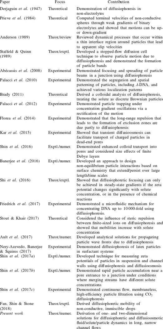
There are many well-known theoretical and empirical results for the drag force on particles as a function of particle shape and the Reynolds number, and numerical simulations provide a means for handling complex particle shapes and boundary effects. Nonetheless, modern research continues to uncover unique particle transport phenomena such as the capture and accumulation of particles and/or bubbles in a variety of flow configurations. For example, a competition between thermophoresis and fluid advection was utilized in a microfluidic set-up to trap particles and concentrate DNA molecules up to 16-fold (Duhr & Braun Reference Duhr and Braun2006). The effect of applied solute gradients on particle-laden flows has also proven to be a source for several novel and unexpected particle dynamics through the action of diffusiophoresis (Prieve et al. Reference Prieve, Anderson, Ebel and Lowell1984). Derjaguin et al. (Reference Derjaguin, Sidorenkov, Zubashchenkov and Kiseleva1947) first introduced the concept of diffusioosmosis in which solute concentration gradients induce slip flows over solid surfaces and extended these ideas to the diffusiophoretic migration of colloidal particles in electrolyte concentration gradients (Derjaguin, Dukhin & Korotkova Reference Derjaguin, Dukhin and Korotkova1961). Since these classic studies of Derjaguin et al., novel particle responses due to the action of diffusiophoresis have been discovered including particle banding (Staffeld & Quinn Reference Staffeld and Quinn1989), particle focusing (Abécassis et al. Reference Abécassis, Cottin-Bizonne, Ybert, Ajdari and Bocquet2008), particle patterning (Palacci et al. Reference Palacci, Abécassis, Cottin-Bizonne, Ybert and Bocquet2010), tuning colloidal interactions (Paustian et al. Reference Paustian, Azevedo, Lundin, Gilkey and Squires2013; Banerjee et al. Reference Banerjee, Williams, Azevedo, Helgeson and Squires2016) and enhanced particle transport in confined geometries (Kar et al. Reference Kar, Chiang, Rivera, Sen and Velegol2015; Shin et al. Reference Shin, Um, Sabass, Ault, Rahimi, Warren and Stone2016; Ault et al. Reference Ault, Warren, Shin and Stone2017). Renewed interest in the diffusiophoretic transport of charged colloidal particles has demonstrated a host of new theoretical methods, experiments and numerical simulations of particle manipulation techniques and systems, some of which are summarized in table 1.
Summary of modern theoretical, experimental and numerical developments regarding diffusiophoresis and applications to the field of fluid dynamics.
Diffusiophoresis refers to the phoretic, spontaneous motion of colloidal particles due to solute gradients. The physical interactions that drive the action of diffusiophoresis can be broken down into two components: chemiphoresis and electrophoresis. Chemiphoresis refers to particle motion due to the osmotic pressure gradient along a particle surface in the presence of local (at the scale of the particle) solute gradients, and electrophoresis refers to the particle motion due to locally developed electric fields as a result of a difference in the diffusivities of the cations and anions. Note that gradients of electrolyte solutions drive diffusiophoresis through the combined influence of chemiphoresis and electrophoresis, whereas gradients of non-electrolyte solutions drive diffusiophoresis solely through the action of chemiphoresis. Diffusioosmosis is a related phenomenon that refers to the effects of chemiphoresis and electrophoresis causing bulk flow adjacent to a stationary surface. In the presence of a local solute gradient
 $\unicode[STIX]{x1D735}c$
, the diffusiophoretic contribution to a particle’s velocity
 $\boldsymbol{u}_{dp}$
relative to the local flow velocity can be written as
 $\boldsymbol{u}_{dp}=\unicode[STIX]{x1D6E4}_{p}\unicode[STIX]{x1D735}\ln c$
, where
 $\unicode[STIX]{x1D6E4}_{p}$
is the so-called diffusiophoretic mobility, which is a function of the particle’s size and zeta potential (Prieve et al.
Reference Prieve, Anderson, Ebel and Lowell1984; Anderson Reference Anderson1989). The nonlinear logarithmic dependence on the solute concentration makes possible the particle banding documented by, for example, Staffeld & Quinn (Reference Staffeld and Quinn1989), Palacci et al. (Reference Palacci, Cottin-Bizonne, Ybert and Bocquet2012) and Shin et al. (Reference Shin, Um, Sabass, Ault, Rahimi, Warren and Stone2016) and the long-lived chemically driven effects document by Abécassis et al. (Reference Abécassis, Cottin-Bizonne, Ybert, Ajdari and Bocquet2008) and Banerjee et al. (Reference Banerjee, Williams, Azevedo, Helgeson and Squires2016).
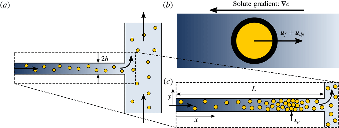
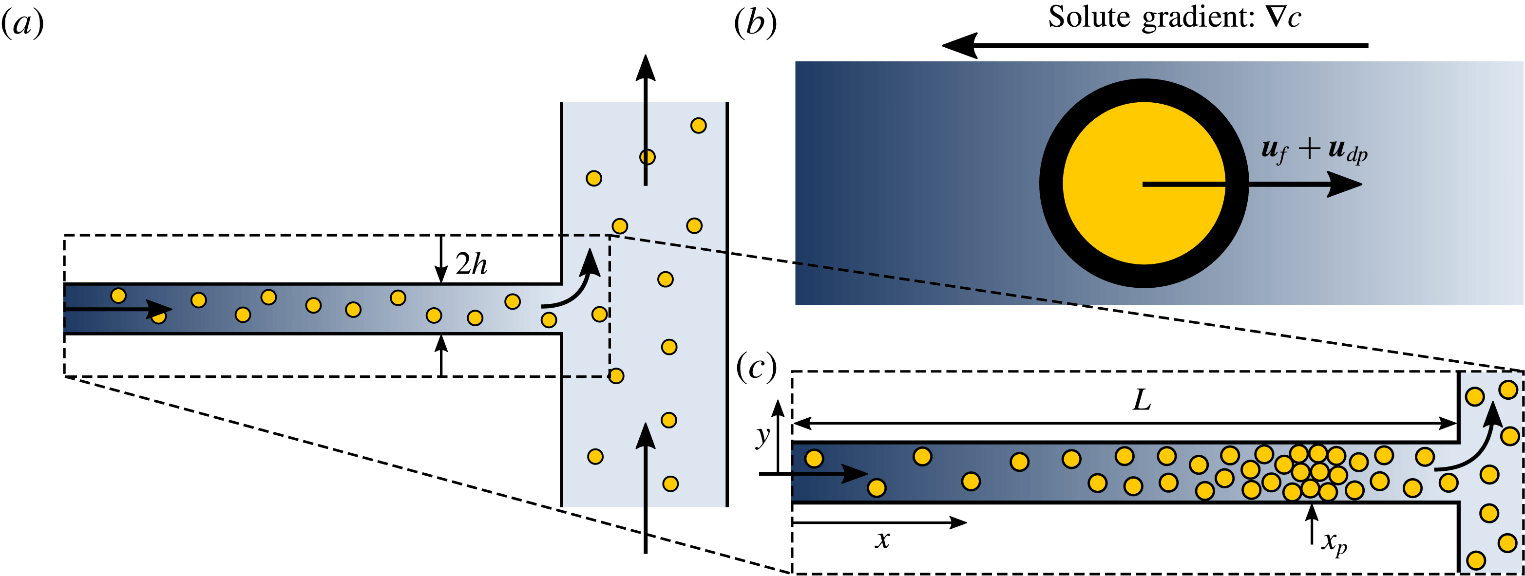
Here, we study the combined influences of diffusiophoresis, diffusioosmosis and fluid advection on particle dynamics in the vicinity of a junction such as the one described in figure 1, in which a fluid stream with one solute concentration merges with a larger main channel that carries a different solute concentration. It is well known that particles under the influence of multiple forces may accumulate when those forces act in opposing directions. For example, such particle accumulation has been observed for the competing effects of thermophoresis versus diffusiophoresis (Maeda, Buguin & Libchaber Reference Maeda, Buguin and Libchaber2011), thermophoresis versus convection (Duhr & Braun Reference Duhr and Braun2006) and electrophoresis versus convection (Stein et al.
Reference Stein, Deurvorst, van der Heyden, Koopmans, Gabel and Dekker2010). More recently, the opposing effects of diffusiophoresis and fluid flow were shown to lead to the rapid accumulation of particles in the vicinity of a flow junction such as shown in figure 1 for appropriately chosen particles and boundary conditions (Abécassis et al.
Reference Abécassis, Cottin-Bizonne, Ybert, Ajdari and Bocquet2008; Shin et al.
Reference Shin, Ault, Warren and Stone2017b
). For example, for particle/solute combinations with
 $\unicode[STIX]{x1D6E4}_{p}>0$
, and a higher solute concentration at the inlet of the side pore such that the solute concentration gradient points upstream in the direction shown in figure 1(b), diffusiophoresis will act to pull particles upstream in the side channel, while fluid advection will act to drive particles downstream. These competing effects can, in some cases, lead to rapid particle accumulation within the pore. However, this accumulation is not the only outcome if the effects are in competition. If, for example, the fluid velocity in the side channel is too low, diffusiophoresis will indeed drive particles upstream in the channel, but they will never reach an equilibrium position. The particles will simply be pumped continuously upstream.
Problem set-up. (a) We consider the fluid/particle/solute dynamics in a narrow pore in the vicinity of a junction with a main channel in which the flow in the pore carries a different solute concentration than that in the main channel. (b) Inside the pore, particle motions are governed by a combination of the fluid velocity
 $\boldsymbol{u}_{f}$
and the diffusiophoretic velocity
 $\boldsymbol{u}_{dp}$
resulting from the solute concentration gradient
 $\unicode[STIX]{x1D735}c$
. (c) With appropriately chosen parameters for the particles of interest, the fluid and diffusiophoretic velocities can be designed to act in opposite directions, resulting in a stable position in the pore
 $x_{p}$
where particles will accumulate. Dark arrows indicate the direction of flow.
In this paper, we use both theory and numerical simulations to quantify and describe the diffusiophoretic particle dynamics in a channel adjacent to a junction, including the recirculatory flows driven by diffusioosmotic effects at the channel walls. For the case of a long, narrow channel, we develop theoretical solutions that can predict the particle dynamics. In § 2, we introduce the coupled set of equations and boundary conditions governing the fluid, solute and particle dynamics. In § 3, we solve for the quasi-one-dimensional solute and particle dynamics in the channel for the case of long, narrow channels. In this limit, it is found that solute/particle dynamics only depends on the average fluid velocity in the channel, and not on the distribution of velocity (i.e. diffusioosmotic effects are negligible). In § 4 we show how this type of system can be used to effectively sort particles by size and/or zeta potential, and we suggest a new approach for performing microfluidic zeta potentiometry of particles. In § 5 we extend this analysis to finite-aspect-ratio channels, and we solve for the two-dimensional fluid, solute and particle dynamics including the effects of diffusioosmosis. In § 6 we introduce the concept of ‘diffusioosmotic pumping’, in which diffusioosmotic effects at the channel walls can be used to drive fluid flow against a net pressure gradient in the side channel for certain parameters. Finally, in § 7 we present conclusions and potential ideas for future work.
2 Governing equations
The transient diffusiophoretic motions of suspended particles are governed by both the fluid and solute profiles in a channel or pore. We model the coupled fluid/solute/particle dynamics with governing equations that include the incompressible Navier–Stokes and continuity equations, an advection–diffusion equation for the solute transport and a diffusiophoretic advection–diffusion equation for the transport of suspended particles. For the following discussion,
 $\unicode[STIX]{x1D70C}$
,
 $\unicode[STIX]{x1D707}$
,
 $p^{\ast }$
and
 $\boldsymbol{u}^{\ast }=(u^{\ast },v^{\ast },w^{\ast })$
are the fluid density, viscosity, pressure and velocity, respectively,
 $c^{\ast }$
and
 $D_{s}$
are the solute concentration and diffusivity, respectively, and
 $n^{\ast }$
,
 $D_{p}$
and
 $\unicode[STIX]{x1D6E4}_{p}$
are the particle concentration, diffusivity and diffusiophoretic mobility, respectively. Throughout this analysis, we will assume that the solute is a single
 $z$
–
 $z$
electrolyte, where
 $z$
is the valence number. In three dimensions, and assuming that the influence of gravity is negligible, the dimensional form of this system of equations is given by
 $$\begin{eqnarray}\displaystyle & \displaystyle \unicode[STIX]{x1D70C}\left(\frac{\unicode[STIX]{x2202}\boldsymbol{u}^{\ast }}{\unicode[STIX]{x2202}t^{\ast }}+\boldsymbol{u}^{\ast }\boldsymbol{\cdot }\unicode[STIX]{x1D735}^{\ast }\boldsymbol{u}^{\ast }\right)=-\unicode[STIX]{x1D735}^{\ast }p^{\ast }+\unicode[STIX]{x1D707}{\unicode[STIX]{x1D735}^{\ast }}^{2}\boldsymbol{u}^{\ast }, & \displaystyle\end{eqnarray}$$
 $$\begin{eqnarray}\displaystyle & \displaystyle \unicode[STIX]{x1D735}^{\ast }\boldsymbol{\cdot }\boldsymbol{u}^{\ast }=0, & \displaystyle\end{eqnarray}$$
 $$\begin{eqnarray}\displaystyle & \displaystyle \frac{\unicode[STIX]{x2202}c^{\ast }}{\unicode[STIX]{x2202}t^{\ast }}+\unicode[STIX]{x1D735}^{\ast }\boldsymbol{\cdot }(\boldsymbol{u}^{\ast }c^{\ast })=D_{s}{\unicode[STIX]{x1D735}^{\ast }}^{2}c^{\ast }, & \displaystyle\end{eqnarray}$$
 $$\begin{eqnarray}\displaystyle & \displaystyle \frac{\unicode[STIX]{x2202}n^{\ast }}{\unicode[STIX]{x2202}t^{\ast }}+\unicode[STIX]{x1D735}^{\ast }\boldsymbol{\cdot }((\boldsymbol{u}^{\ast }+\boldsymbol{u}_{dp}^{\ast })n^{\ast })=D_{p}{\unicode[STIX]{x1D735}^{\ast }}^{2}n^{\ast }, & \displaystyle\end{eqnarray}$$
 $^{\ast }$
denote dimensional quantities. Note that, in writing the particle concentration equation as (2.1d
), we have assumed that there are no other dynamical effects for the particles, i.e. the Stokes number for the particles is small. Thus, the velocity of individual particles can be approximated as the sum of the local fluid advection velocity and the diffusiophoretic velocity component
 $\boldsymbol{u}_{dp}^{\ast }$
based on the local solute concentration. Here,
 $\boldsymbol{u}_{dp}^{\ast }=\unicode[STIX]{x1D6E4}_{p}\unicode[STIX]{x1D735}^{\ast }\ln c^{\ast }$
represents the diffusiophoretic velocity of a particle due to gradients in the logarithm of the solute concentration (Prieve et al.
Reference Prieve, Anderson, Ebel and Lowell1984; Anderson Reference Anderson1989). This logarithmic ‘sensing’ of the solute concentration by the particles is responsible for the rapid focusing of particles that has been observed extensively in solute concentration gradients, and also explains why diffusiophoretic particle motions can persist for surprisingly long time scales compared to the time scale for solute diffusion, i.e. although the solute concentration gradient may be small,
 $\unicode[STIX]{x1D735}^{\ast }\ln c^{\ast }$
may be large (Palacci et al.
Reference Palacci, Cottin-Bizonne, Ybert and Bocquet2012). Equations (2.1a
)–(2.1d
) form a coupled system of equations that govern the diffusiophoretic motion of charged colloidal particles in general three-dimensional flows. This set of equations is to be solved for given boundary and initial conditions, for example, a given particle
 $n$
and salt
 $c$
concentration at
 $x=0$
, where the channel begins (see figure 1). With (2.1a
)–(2.1c
), and including boundary conditions that can include diffusioosmotic slip, in principle
 $\boldsymbol{u}^{\ast }$
and
 $c^{\ast }$
can be determined, after which (2.1d
) gives the evolution of
 $n$
.
2.1 Non-dimensional equations
Before proceeding to examine the fluid/solute/particle dynamics in long, narrow pores of height
 $2h$
and length
 $L\gg h$
, we first non-dimensionalize the system of governing equations. The average fluid speed in the pores is denoted
 $\bar{U}$
. We restrict ourselves to two dimensions and non-dimensionalize the system of governing equations for the fluid velocity
 $\boldsymbol{u}^{\ast }=(u^{\ast },v^{\ast })$
as follows:
 $$\begin{eqnarray}\left.\begin{array}{@{}c@{}}\displaystyle t=\frac{t^{\ast }D_{s}}{L^{2}},\quad x=\frac{x^{\ast }}{L},\quad y=\frac{y^{\ast }}{h},\quad u=\frac{u^{\ast }}{\bar{U}},\quad v=\frac{v^{\ast }L}{\bar{U}h},\quad n=\frac{n^{\ast }}{n_{c}},\\ \displaystyle c=\frac{c^{\ast }}{c_{c}},\quad \text{and}\quad p=\frac{p^{\ast }h^{2}}{\unicode[STIX]{x1D707}\bar{U}L},\end{array}\right\}\end{eqnarray}$$
where
 $n_{c}=n^{\ast }(x=0)$
and
 $c_{c}=c^{\ast }(x=0)$
. With these non-dimensionalizations and considering the channel configuration shown in figure 1, the governing equations can be rewritten as
 $$\begin{eqnarray}\displaystyle & \displaystyle \unicode[STIX]{x1D716}^{2}\frac{D_{s}}{\unicode[STIX]{x1D708}}\frac{\unicode[STIX]{x2202}u}{\unicode[STIX]{x2202}t}+\unicode[STIX]{x1D716}Re\left(u\frac{\unicode[STIX]{x2202}u}{\unicode[STIX]{x2202}x}+v\frac{\unicode[STIX]{x2202}u}{\unicode[STIX]{x2202}y}\right)=-\frac{\unicode[STIX]{x2202}p}{\unicode[STIX]{x2202}x}+\unicode[STIX]{x1D716}^{2}\frac{\unicode[STIX]{x2202}^{2}u}{\unicode[STIX]{x2202}x^{2}}+\frac{\unicode[STIX]{x2202}^{2}u}{\unicode[STIX]{x2202}y^{2}}, & \displaystyle\end{eqnarray}$$
 $$\begin{eqnarray}\displaystyle & \displaystyle \unicode[STIX]{x1D716}^{4}\frac{D_{s}}{\unicode[STIX]{x1D708}}\frac{\unicode[STIX]{x2202}v}{\unicode[STIX]{x2202}t}+\unicode[STIX]{x1D716}^{3}Re\left(u\frac{\unicode[STIX]{x2202}v}{\unicode[STIX]{x2202}x}+v\frac{\unicode[STIX]{x2202}v}{\unicode[STIX]{x2202}y}\right)=-\frac{\unicode[STIX]{x2202}p}{\unicode[STIX]{x2202}y}+\unicode[STIX]{x1D716}^{4}\frac{\unicode[STIX]{x2202}^{2}v}{\unicode[STIX]{x2202}x^{2}}+\unicode[STIX]{x1D716}^{2}\frac{\unicode[STIX]{x2202}^{2}v}{\unicode[STIX]{x2202}y^{2}}, & \displaystyle\end{eqnarray}$$
 $$\begin{eqnarray}\displaystyle & \displaystyle \frac{\unicode[STIX]{x2202}u}{\unicode[STIX]{x2202}x}+\frac{\unicode[STIX]{x2202}v}{\unicode[STIX]{x2202}y}=0, & \displaystyle\end{eqnarray}$$
 $$\begin{eqnarray}\displaystyle & \displaystyle \unicode[STIX]{x1D716}^{2}\frac{\unicode[STIX]{x2202}c}{\unicode[STIX]{x2202}t}+Pe_{s}\unicode[STIX]{x1D716}^{2}\left(u\frac{\unicode[STIX]{x2202}c}{\unicode[STIX]{x2202}x}+v\frac{\unicode[STIX]{x2202}c}{\unicode[STIX]{x2202}y}\right)=\unicode[STIX]{x1D716}^{2}\frac{\unicode[STIX]{x2202}^{2}c}{\unicode[STIX]{x2202}x^{2}}+\frac{\unicode[STIX]{x2202}^{2}c}{\unicode[STIX]{x2202}y^{2}}, & \displaystyle\end{eqnarray}$$
 $$\begin{eqnarray}\displaystyle & \displaystyle \unicode[STIX]{x1D716}^{2}\frac{D_{s}}{D_{p}}\left[\frac{\unicode[STIX]{x2202}n}{\unicode[STIX]{x2202}t}+Pe_{s}\left(\frac{\unicode[STIX]{x2202}(u_{p}n)}{\unicode[STIX]{x2202}x}+\frac{\unicode[STIX]{x2202}(v_{p}n)}{\unicode[STIX]{x2202}y}\right)\right]=\unicode[STIX]{x1D716}^{2}\frac{\unicode[STIX]{x2202}^{2}n}{\unicode[STIX]{x2202}x^{2}}+\frac{\unicode[STIX]{x2202}^{2}n}{\unicode[STIX]{x2202}y^{2}}, & \displaystyle\end{eqnarray}$$
 $Re=\bar{U}h/\unicode[STIX]{x1D708}$
is the flow Reynolds number,
 $Pe_{s}=L\bar{U}/D_{s}$
is the solute Péclet number,
 $\unicode[STIX]{x1D716}=h/L$
and
 $\boldsymbol{u}_{p}=\boldsymbol{u}+\boldsymbol{u}_{dp}$
is the particle velocity due to fluid advection and diffusiophoresis, i.e.
 $$\begin{eqnarray}u_{p}=u+\frac{\unicode[STIX]{x1D6E4}_{p}}{L\bar{U}}\frac{\unicode[STIX]{x2202}\ln c}{\unicode[STIX]{x2202}x}\quad \text{and}\quad v_{p}=v+\frac{1}{\unicode[STIX]{x1D716}^{2}}\frac{\unicode[STIX]{x1D6E4}_{p}}{L\bar{U}}\frac{\unicode[STIX]{x2202}\ln c}{\unicode[STIX]{x2202}y}.\end{eqnarray}$$
2.2 Boundary and initial conditions
The solution of (2.3) is subject to boundary conditions on the fluid, solute and particle dynamics. These boundary conditions are summarized by:
 $$\begin{eqnarray}\displaystyle & \displaystyle \text{No fluid penetration at the walls:}~v(x,\pm 1,t)=0, & \displaystyle\end{eqnarray}$$
 $$\begin{eqnarray}\displaystyle & \displaystyle \text{Fixed outlet pressure:}~p(1,y,t)=0, & \displaystyle\end{eqnarray}$$
 $$\begin{eqnarray}\displaystyle & \displaystyle \!\!\text{Fixed inlet and outlet solute concentrations:}~c(0,y,t)=1~\text{and}~c(1,y,t)=\unicode[STIX]{x1D6FD},\hspace{16.49995pt} & \displaystyle\end{eqnarray}$$
 $$\begin{eqnarray}\displaystyle & \displaystyle \text{Fixed inlet and outlet particle concentrations:}~n(0,y,t)=n(1,y,t)=1, & \displaystyle\end{eqnarray}$$
 $$\begin{eqnarray}\displaystyle & \displaystyle \text{No-flux conditions at the channel walls:}~\frac{\unicode[STIX]{x2202}c}{\unicode[STIX]{x2202}y}=\frac{\unicode[STIX]{x2202}n}{\unicode[STIX]{x2202}y}=0\quad \text{at }y=\pm 1, & \displaystyle\end{eqnarray}$$
 $$\begin{eqnarray}\displaystyle & \displaystyle \text{Symmetry conditions:}~\frac{\unicode[STIX]{x2202}u}{\unicode[STIX]{x2202}y}=\frac{\unicode[STIX]{x2202}p}{\unicode[STIX]{x2202}y}=\frac{\unicode[STIX]{x2202}c}{\unicode[STIX]{x2202}y}=\frac{\unicode[STIX]{x2202}n}{\unicode[STIX]{x2202}y}=v=0\quad \text{at }y=0, & \displaystyle\end{eqnarray}$$
 $$\begin{eqnarray}\displaystyle & \displaystyle \text{Fixed average fluid velocity:}~\int _{y=0}^{y=1}u(x,y,t)\,\text{d}y=1, & \displaystyle\end{eqnarray}$$
 $$\begin{eqnarray}\displaystyle & \displaystyle \text{Diffusioosmotic wall slip condition:}~u(x,\pm 1,t)=u_{w}(x,t)=-\left.\frac{\unicode[STIX]{x1D6E4}_{w}}{L\bar{U}}\frac{\unicode[STIX]{x2202}\ln c}{\unicode[STIX]{x2202}x}\right|_{y=\pm 1}.\qquad & \displaystyle\end{eqnarray}$$
 $\unicode[STIX]{x1D6E4}_{w}$
is the diffusioosmotic mobility of the wall, and the minus sign is because we are now interested in the motion of the fluid, whereas with diffusiophoresis the focus is on the motion of the particle. As initial conditions, we assume an initially uniform distribution of particles throughout the channel, i.e.
 $n(x,y,0)=1$
. In later sections, we will show that the transient solute dynamics occurs much faster than the transient particle dynamics. Thus, for the purposes of modelling the diffusiophoretic particle motions, we may assume either an initially uniform solute concentration profile, i.e.
 $c(x,y,0)=1$
, or we can simply directly impose the fully developed solute concentration profile as the initial condition. With these boundary and initial conditions and the non-dimensional governing equations given by (2.3), we next seek solutions for the fluid/solute/particle dynamics in long, narrow pores through the application of the lubrication approximation.
Note that, by assuming uniform pressure and solute concentration profiles at
 $x=1$
, we have assumed that any ‘end effects’ due to the presence of the junction are negligible. Of course, such an assumption is generally invalid, and the main channel flow must in turn affect the fluid/solute/particle dynamics within the pore. It is perhaps more appropriate to describe this boundary condition as ‘effective’ in nature, such that the outlet is not located exactly at
 $x=1$
. However, because we have assumed that the channel has a large aspect ratio, i.e.
 $h/L\ll 1$
, this deviation is negligible, and we effectively have uniform boundary conditions at
 $x=1$
, which we have also confirmed with three-dimensional numerical simulations.
2.3 Assumption of constant
 $\unicode[STIX]{x1D6E4}_{p}$
and
$\unicode[STIX]{x1D6E4}_{w}$


Throughout this analysis, we will make the assumption of constant diffusiophoretic and diffusioosmotic mobilities,
 $\unicode[STIX]{x1D6E4}_{p}$
and
 $\unicode[STIX]{x1D6E4}_{w}$
. This assumption is found frequently throughout the literature due to the convenient analytical results that it makes possible, and is generally valid for the case of dilute solute concentrations. Kirby & Hasselbrink (Reference Kirby and Hasselbrink2004) suggest that for a wide range of concentrations, the zeta potential
 $\unicode[STIX]{x1D701}$
is proportional to the log of the solute concentration for symmetric electrolytes with a valence of
 $z=1$
, i.e.
 $\unicode[STIX]{x1D701}\propto \ln c$
. Thus, for cases where the dilute solute assumption is not valid, we must generally consider the variation of the zeta potential as a function of solute concentration, and thus we must consider the variability of
 $\unicode[STIX]{x1D6E4}_{p}$
and
 $\unicode[STIX]{x1D6E4}_{w}$
. However, for dilute solute concentrations we can safely neglect the variation in zeta potential. For example, the zeta potential difference between 100 and 10 mM solute concentration solutions is approximately 50 %, whereas the zeta potential difference between 100 and
 $10~\unicode[STIX]{x03BC}\text{M}$
solute concentration solutions is only approximately 20 %. Considering this variability of zeta potential will greatly limit the amount of theoretical progress that may be achieved towards analytical results, and so we limit ourselves to the assumption of dilute solute concentrations and leave the additional analysis that considers variable zeta potentials to future work.
3 Diffusiophoresis in quasi-one-dimensional pores
We consider the motion of colloidal particles under the combined influences of fluid flow and solute gradients in long, narrow channel geometries such as illustrated in figure 1. For sufficiently long, narrow geometries, the diffusiophoretic particle dynamics is well approximated by a one-dimensional model. While in general the fluid velocity and pressure, as well as the solute and particle concentrations, will all be functions of
 $x$
,
 $y$
and
 $t$
in a channel flow, i.e.
 $\boldsymbol{u}(x,y,t)$
,
 $p(x,y,t)$
,
 $c(x,y,t)$
and
 $n(x,y,t)$
, the lubrication approximation may be used to show that both the solute and particle concentrations are independent of
 $y$
to leading order for high-aspect-ratio channels, i.e.
 $\unicode[STIX]{x1D716}=h/L\ll 1$
.
We consider low-Reynolds-number flows (
 $Re\ll 1$
) and seek the leading-order dynamics through a formal expansion with the small parameter
 $\unicode[STIX]{x1D716}$
. As can be seen in the non-dimensionalized governing equations (2.3), with
 $Re\ll 1$
, only
 $\unicode[STIX]{x1D716}^{2}$
appears. So, we seek solutions of the form
 $$\begin{eqnarray}\displaystyle & \displaystyle u(x,y,t)=u_{0}+\unicode[STIX]{x1D716}^{2}u_{1}+\unicode[STIX]{x1D716}^{4}u_{2}+\unicode[STIX]{x1D716}^{6}u_{3}+\cdots \,, & \displaystyle\end{eqnarray}$$
 $$\begin{eqnarray}\displaystyle & \displaystyle v(x,y,t)=v_{0}+\unicode[STIX]{x1D716}^{2}v_{1}+\unicode[STIX]{x1D716}^{4}v_{2}+\unicode[STIX]{x1D716}^{6}v_{3}+\cdots \,, & \displaystyle\end{eqnarray}$$
 $$\begin{eqnarray}\displaystyle & \displaystyle p(x,y,t)=p_{0}+\unicode[STIX]{x1D716}^{2}p_{1}+\unicode[STIX]{x1D716}^{4}p_{2}+\unicode[STIX]{x1D716}^{6}p_{3}+\cdots \,, & \displaystyle\end{eqnarray}$$
 $$\begin{eqnarray}\displaystyle & \displaystyle c(x,y,t)=c_{0}+\unicode[STIX]{x1D716}^{2}c_{1}+\unicode[STIX]{x1D716}^{4}c_{2}+\unicode[STIX]{x1D716}^{6}c_{3}+\cdots \,, & \displaystyle\end{eqnarray}$$
 $$\begin{eqnarray}\displaystyle & \displaystyle n(x,y,t)=n_{0}+\unicode[STIX]{x1D716}^{2}n_{1}+\unicode[STIX]{x1D716}^{4}n_{2}+\unicode[STIX]{x1D716}^{6}n_{3}+\cdots \,, & \displaystyle\end{eqnarray}$$
 $u_{i}$
,
 $v_{i}$
,
 $p_{i}$
,
 $c_{i}$
and
 $n_{i}$
may be functions of
 $x$
,
 $y$
and
 $t$
. To leading order, the non-dimensional governing equations given by (2.3) become
 $$\begin{eqnarray}\frac{\unicode[STIX]{x2202}^{2}u_{0}}{\unicode[STIX]{x2202}y^{2}}-\frac{\unicode[STIX]{x2202}p_{0}}{\unicode[STIX]{x2202}x}=0,\quad \frac{\unicode[STIX]{x2202}p_{0}}{\unicode[STIX]{x2202}y}=0,\quad \frac{\unicode[STIX]{x2202}u_{0}}{\unicode[STIX]{x2202}x}+\frac{\unicode[STIX]{x2202}v_{0}}{\unicode[STIX]{x2202}y}=0,\quad \frac{\unicode[STIX]{x2202}^{2}c_{0}}{\unicode[STIX]{x2202}y^{2}}=0,\quad \text{and}\quad \frac{\unicode[STIX]{x2202}^{2}n_{0}}{\unicode[STIX]{x2202}y^{2}}=0.\end{eqnarray}$$
Integrating the last two of these and applying the no-flux boundary condition given by (2.5e
), we find that
 $c_{0}=c_{0}(x,t)$
and
 $n_{0}=n_{0}(x,t)$
, i.e. the solute and particle concentrations are independent of
 $y$
to leading order. We further see that
 $p_{0}=p_{0}(x,t)$
, and the pressure is also independent of
 $y$
to leading order, as expected by the lubrication approximation. Thus, the effects of diffusioosmosis on the solute and particle concentrations and on the pressure are negligible to leading order, and only the mean flow velocity
 $\bar{U}$
affects the leading-order solute and particle distributions. Substituting these results into (2.3d
) and (2.3e
) we find to leading order
 $$\begin{eqnarray}\frac{\unicode[STIX]{x2202}c_{0}}{\unicode[STIX]{x2202}t}+Pe_{s}u_{0}\frac{\unicode[STIX]{x2202}c_{0}}{\unicode[STIX]{x2202}x}-\frac{\unicode[STIX]{x2202}^{2}c_{0}}{\unicode[STIX]{x2202}x^{2}}-\frac{\unicode[STIX]{x2202}^{2}c_{1}}{\unicode[STIX]{x2202}y^{2}}=0,\end{eqnarray}$$
 $$\begin{eqnarray}\displaystyle & & \displaystyle \frac{\unicode[STIX]{x2202}n_{0}}{\unicode[STIX]{x2202}t}-\frac{\unicode[STIX]{x1D6E4}_{p}}{D_{s}}n_{0}\left(\frac{\unicode[STIX]{x2202}\ln c_{0}}{\unicode[STIX]{x2202}x}\right)^{2}+Pe_{s}u_{0}\frac{\unicode[STIX]{x2202}n_{0}}{\unicode[STIX]{x2202}x}+\frac{\unicode[STIX]{x1D6E4}_{p}}{D_{s}}\frac{\unicode[STIX]{x2202}n_{0}}{\unicode[STIX]{x2202}x}\frac{\unicode[STIX]{x2202}\ln c_{0}}{\unicode[STIX]{x2202}x}+\frac{\unicode[STIX]{x1D6E4}_{p}}{D_{s}}\frac{n_{0}}{c_{0}}\frac{\unicode[STIX]{x2202}^{2}c_{0}}{\unicode[STIX]{x2202}x^{2}}-\frac{D_{p}}{D_{s}}\frac{\unicode[STIX]{x2202}^{2}n_{0}}{\unicode[STIX]{x2202}x^{2}}\nonumber\\ \displaystyle & & \displaystyle \quad +\,Pe_{s}n_{0}\frac{\unicode[STIX]{x2202}v_{0}}{\unicode[STIX]{x2202}y}+\frac{\unicode[STIX]{x1D6E4}_{p}}{D_{s}}\frac{n_{0}}{c_{0}}\frac{\unicode[STIX]{x2202}^{2}c_{1}}{\unicode[STIX]{x2202}y^{2}}-\frac{D_{p}}{D_{s}}\frac{\unicode[STIX]{x2202}^{2}n_{1}}{\unicode[STIX]{x2202}y^{2}}+Pe_{s}n_{0}\frac{\unicode[STIX]{x2202}u_{0}}{\unicode[STIX]{x2202}x}=0.\end{eqnarray}$$
 $c_{1}$
and
 $n_{1}$
and we find
 $$\begin{eqnarray}\displaystyle & \displaystyle \frac{\unicode[STIX]{x2202}c_{0}}{\unicode[STIX]{x2202}t}+Pe_{s}\frac{\unicode[STIX]{x2202}c_{0}}{\unicode[STIX]{x2202}x}-\frac{\unicode[STIX]{x2202}^{2}c_{0}}{\unicode[STIX]{x2202}x^{2}}=0, & \displaystyle\end{eqnarray}$$
 $$\begin{eqnarray}\displaystyle & \displaystyle \frac{\unicode[STIX]{x2202}n_{0}}{\unicode[STIX]{x2202}t}+\frac{\unicode[STIX]{x2202}}{\unicode[STIX]{x2202}x}\left[\left(Pe_{s}+\frac{\unicode[STIX]{x1D6E4}_{p}}{D_{s}}\frac{\unicode[STIX]{x2202}\ln c_{0}}{\unicode[STIX]{x2202}x}\right)n_{0}\right]-\frac{D_{p}}{D_{s}}\frac{\unicode[STIX]{x2202}^{2}n_{0}}{\unicode[STIX]{x2202}x^{2}}=0, & \displaystyle\end{eqnarray}$$
Before we attempt to solve this system, we first comment on the relevant time scales of the physical processes. First, note that we focus on solute Péclet numbers that are
 $Pe_{s}=O(1)$
. We will show below that this magnitude of Péclet numbers tends to locate the accumulating particle peak near the centre of the channel for typical values of
 $\unicode[STIX]{x1D6E4}_{p}/D_{s}$
and
 $\unicode[STIX]{x1D6FD}$
, and also provides the best separation dynamics for applications with multiple types of particles. Then, with
 $Pe_{s}=O(1)$
, equation (3.4a
) shows that the solute concentration profile
 $c_{0}$
evolves on a time scale
 $O(1)$
. Furthermore, with the imposed boundary conditions,
 $c_{0}$
will approach a steady-state distribution, and thus we expect
 $\unicode[STIX]{x2202}c_{0}/\unicode[STIX]{x2202}t\approx 0$
for
 $t\gg 1$
. However, the diffusive term in (3.4b
) is
 $O(D_{p}/D_{s})$
. Since we expect the formation of a peak in the particle concentration within the channel, where diffusion must play a significant role, we thus expect that the accumulation dynamics of the particles occurs over a much longer time scale, since
 $D_{s}/D_{p}$
is typically
 $O(10^{3})$
for common combinations of solutes and particles. With this reasoning, and with supporting results from numerical simulations to be provided below, we assume that the solute concentration profile is steady over the relevant time scale of particle accumulation. That is, we solve the slightly modified system
 $$\begin{eqnarray}\displaystyle & \displaystyle Pe_{s}\frac{\text{d}c_{0}}{\text{d}x}-\frac{\text{d}^{2}c_{0}}{\text{d}x^{2}}=0, & \displaystyle\end{eqnarray}$$
 $$\begin{eqnarray}\displaystyle & \displaystyle \frac{\unicode[STIX]{x2202}n_{0}}{\unicode[STIX]{x2202}t}+\frac{\unicode[STIX]{x2202}}{\unicode[STIX]{x2202}x}\left[\left(Pe_{s}+\frac{\unicode[STIX]{x1D6E4}_{p}}{D_{s}}\frac{\text{d}\ln c_{0}}{\text{d}x}\right)n_{0}\right]-\frac{D_{p}}{D_{s}}\frac{\unicode[STIX]{x2202}^{2}n_{0}}{\unicode[STIX]{x2202}x^{2}}=0, & \displaystyle\end{eqnarray}$$
 $c_{0}=c_{0}(x)$
. As summarized in § 2.2, the solution of (3.5) is subject to
 $c_{0}(0)=1$
,
 $c_{0}(1)=\unicode[STIX]{x1D6FD}$
, and
 $n_{0}(0,t)=n_{0}(1,t)=1$
. In addition to
 $\unicode[STIX]{x1D6FD}$
and
 $Pe_{s}$
, equation (3.5b
) is governed by two additional non-dimensional parameters:
 $\unicode[STIX]{x1D6E4}_{p}/D_{s}$
, which determines the rate of particle diffusiophoresis relative to solute diffusion, and
 $D_{p}/D_{s}$
, which determines the rate of particle diffusion relative to solute diffusion.
Equation (3.5a ) has a straightforward solution given by
 $$\begin{eqnarray}c_{0}(x)=\frac{\unicode[STIX]{x1D6FD}-1}{\text{e}^{Pe_{s}}-1}(\text{e}^{Pe_{s}x}-1)+1.\end{eqnarray}$$
In the limit of
 $Pe_{s}\rightarrow 0$
, solute diffusion dominates, and
 $c_{0}(x)$
approaches a linear profile. However, for
 $Pe_{s}\rightarrow \infty$
, the solute concentration approaches
 $c_{0}(x)=1$
throughout the pore, except for a shrinking region near the outlet where steeper and steeper solute concentration gradients develop. With the solution for the solute concentration given by (3.6), the diffusiophoretic contribution to (3.5b
) is known analytically, and (3.5b
) can be solved to yield the transient leading-order particle concentration
 $n_{0}$
. We seek intuition towards an analytical solution approach for (3.5b
) by performing one-dimensional (1-D) numerical simulations of the full governing equations (2.1). We assume an initial particle concentration distribution of
 $n(\boldsymbol{x},0)=1$
. Furthermore, because of the time scale arguments previously mentioned, we assume an initial solute concentration profile given by (3.6), i.e. we impose the leading-order steady-state solute concentration profile as the initial condition in our 1-D simulations. Assuming instead, for example, an initial uniform solute concentration of
 $c=1$
has a negligible influence on the particle dynamics because the solute quickly evolves towards (3.6) within
 $t=O(1)$
.
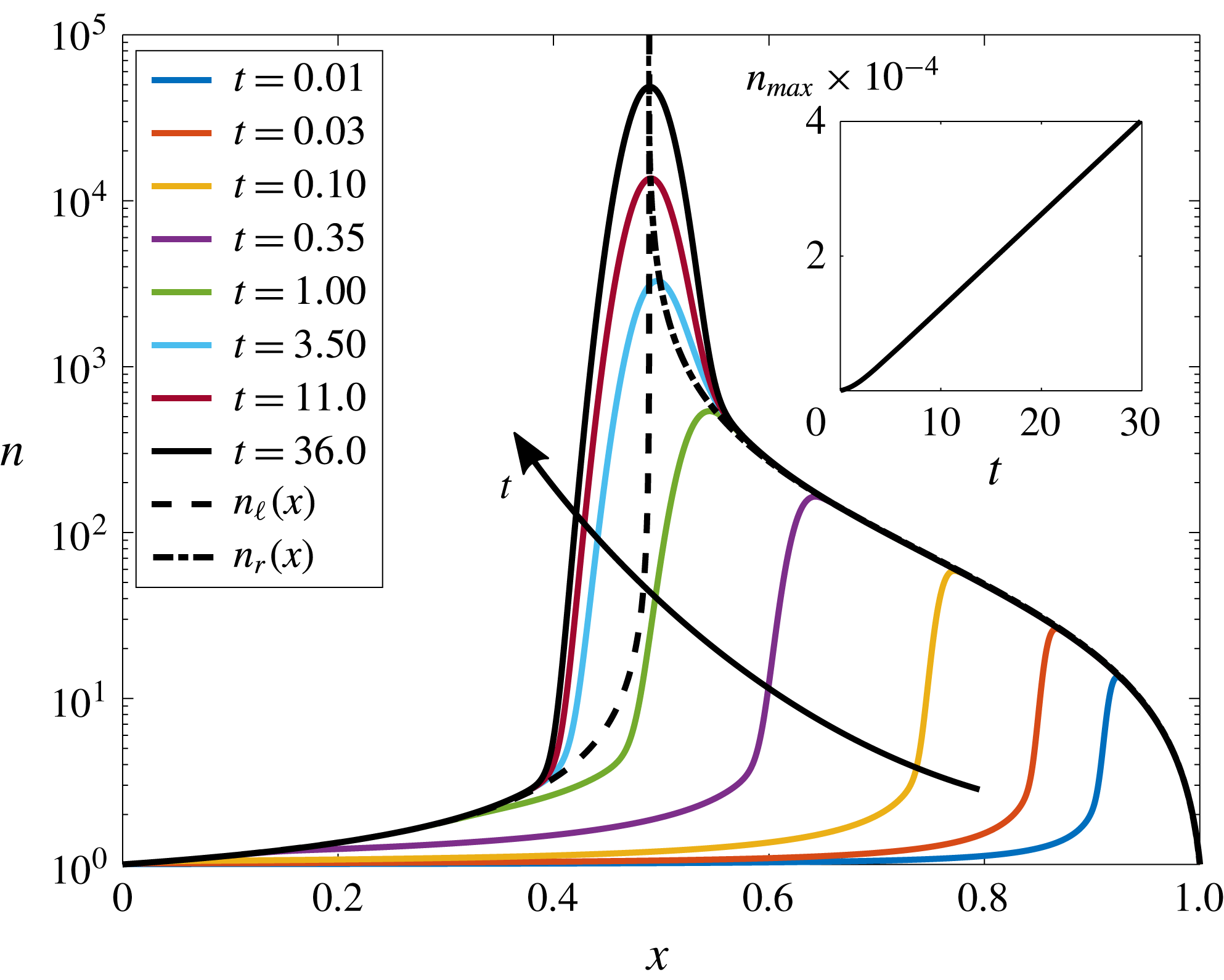
Typical numerical simulations of the 1-D particle dynamics are shown in figure 2. As can be seen, for typical, physically realistic non-dimensional parameters, the particle concentration initially forms a peak near the outlet that then moves upstream and approaches a steady location within
 $t=O(1)$
. After this initial transient period, the dynamics approaches an asymptotic behaviour in which the particle concentration can apparently be described by three separate solutions, each valid in a certain region. The location of the particle concentration peak approaches a steady position, and the peak grows larger in time (we will show that this growth is linear in
 $t$
until the maximum packing fraction is approached and short-range interactions dominate), whereas upstream and downstream of the peak the particle concentrations are steady and independent of time.
Typical suspended particle concentrations
 $n$
for
 $Pe_{s}=0.75$
,
 $D_{p}/D_{s}=6.25\times 10^{-4}$
,
 $\unicode[STIX]{x1D6E4}_{p}/D_{s}=0.475$
and
 $\unicode[STIX]{x1D6FD}=0.01$
. Dimensionless parameters were chosen to reflect typical physical conditions. At early times, the particle concentration increases everywhere inside the pore as particles are brought in at both
 $x=0$
and
 $x=1$
. The profile quickly develops a peak at a pore position
 $x_{p}(t)$
. To the left and right of the peak, particle diffusion is negligible, and
 $n$
quickly approaches the steady-state solutions
 $n_{\ell }(x)$
and
 $n_{r}(x)$
in those regions of the pore, whereas the peak itself grows linearly in time as we will show. The figure inset shows the growth of the peak particle concentration in the channel
 $n_{max}$
. As can be seen, this growth is linear in time except for a brief initial development period that is
 $t=O(1)$
.
Furthermore, because
 $D_{p}/D_{s}\ll 1$
for typical combinations of solute and particles, and because gradients of
 $n$
are relatively small in the regions upstream and downstream of the peak, we first seek steady-state solutions to (3.5b
) with negligible particle diffusivity, i.e. we seek solutions to
 $$\begin{eqnarray}\frac{\text{d}}{\text{d}x}\left[\left(1+\frac{\unicode[STIX]{x1D6E4}_{p}}{L\bar{U}}\frac{\text{d}\ln c_{0}}{\text{d}x}\right)n_{l,r}\right]=0,\end{eqnarray}$$
where
 $n_{\ell }$
and
 $n_{r}$
denote the steady-state particle concentrations to the left and right of the peak, respectively.
Analytical solutions to (3.7) for the particle concentrations upstream and downstream of the peak, i.e.
 $n_{\ell }(x)$
and
 $n_{r}(x)$
, respectively, each satisfying one boundary condition at the inlet or outlet, are given by
 $$\begin{eqnarray}\displaystyle & \displaystyle n_{\ell }(x)=F(x)\frac{\displaystyle \text{e}^{Pe_{s}}+\frac{\unicode[STIX]{x1D6E4}_{p}}{D_{s}}(\unicode[STIX]{x1D6FD}-1)-1}{\text{e}^{Pe_{s}}-1}, & \displaystyle\end{eqnarray}$$
 $$\begin{eqnarray}\displaystyle & \displaystyle n_{r}(x)=F(x)\frac{\displaystyle \text{e}^{Pe_{s}}\left(\frac{\unicode[STIX]{x1D6E4}_{p}}{D_{s}}(\unicode[STIX]{x1D6FD}-1)+\unicode[STIX]{x1D6FD}\right)-\unicode[STIX]{x1D6FD}}{(\text{e}^{Pe_{s}}-1)\unicode[STIX]{x1D6FD}}, & \displaystyle\end{eqnarray}$$
 $$\begin{eqnarray}F(x)=\frac{\text{e}^{Pe_{s}}+\text{e}^{Pe_{s}x}(\unicode[STIX]{x1D6FD}-1)-\unicode[STIX]{x1D6FD}}{\displaystyle \text{e}^{Pe_{s}}+\text{e}^{Pe_{s}x}\left(1+\frac{\unicode[STIX]{x1D6E4}_{p}}{D_{s}}\right)(\unicode[STIX]{x1D6FD}-1)-\unicode[STIX]{x1D6FD}}.\end{eqnarray}$$
Because the solutions
 $n_{\ell }(x)$
and
 $n_{r}(x)$
satisfy the particle-diffusion-free equation (3.7), they only satisfy the upstream and downstream boundary conditions, respectively. Both solutions diverge at the steady-state peak location,
 $x_{p}^{\infty }$
, which is given by
 $F(x_{p}^{\infty })\rightarrow \infty$
or
 $$\begin{eqnarray}x_{p}^{\infty }=Pe_{s}^{-1}\ln \left[\frac{\unicode[STIX]{x1D6FD}-\text{e}^{Pe_{s}}}{\displaystyle \left(1+\frac{\unicode[STIX]{x1D6E4}_{p}}{D_{s}}\right)(\unicode[STIX]{x1D6FD}-1)}\right].\end{eqnarray}$$
This peak location can be understood as the location in the flow where the advective velocity exactly balances the diffusiophoretic velocity, such that particles accumulate. As can be seen from (3.10), for a given particle and solute, i.e. for fixed
 $\unicode[STIX]{x1D6E4}_{p}/D_{s}$
, the flow parameters
 $Pe_{s}$
and
 $\unicode[STIX]{x1D6FD}$
can be tuned to drive particle accumulation at any location in the channel. This feature is shown graphically in figure 3, where the position of the particle peak within the channel is shown as a function of
 $Pe_{s}$
for a range of
 $\unicode[STIX]{x1D6E4}_{p}/D_{s}$
. Equation (3.10) demonstrates why we limit our focus to
 $Pe_{s}=O(1)$
. Assuming
 $\unicode[STIX]{x1D6FD}\ll 1$
and rearranging, we find that
 $Pe_{s}=\ln (1+\unicode[STIX]{x1D6E4}_{p}/D_{s})/(1-x_{p}^{\infty })$
. Then with
 $x_{p}^{\infty }\approx 0.5$
, i.e. fixing the particle accumulation near the centre of the channel, for typical values of
 $\unicode[STIX]{x1D6E4}_{p}/D_{s}=O(1)$
we also have
 $Pe_{s}=O(1)$
. Much smaller or larger values of
 $Pe_{s}$
will shift the particle dynamics towards the channel inlet or outlet, respectively.
Steady-state peak particle concentration location
 $x_{p}^{\infty }$
in the channel as a function of the solute Péclet number
 $Pe_{s}$
for a variety of particle diffusiophoretic mobilities
 $\unicode[STIX]{x1D6E4}_{p}/D_{s}$
for
 $\unicode[STIX]{x1D6FD}=0.01$
. For a given
 $\unicode[STIX]{x1D6E4}_{p}/D_{s}$
, both
 $Pe_{s}$
and
 $\unicode[STIX]{x1D6FD}$
can be tuned to selectively determine the channel position at which particles accumulate. Note that for
 $x_{p}^{\infty }<0$
, particle diffusiophoresis is too strong relative to fluid advection, and particles will be continuously pumped upstream without accumulating in the channel. Also note that
 $\unicode[STIX]{x1D6E4}_{p}/D_{s}<1$
for most realistic combinations of solute and particles.

With analytical expressions for the steady-state particle concentrations at the inlet and outlet of the channel, we can directly calculate the in/out-flow of particles at both the inlet and at the outlet. Using the analytical solutions for
 $n_{\ell }(x)$
and
 $n_{r}(x)$
given by (3.8), it is straightforward to show that these fluxes are not equal except for the trivial case of
 $\unicode[STIX]{x1D6E4}_{p}/D_{s}=0$
. However, with
 $\unicode[STIX]{x1D6E4}_{p}/D_{s}>0$
and
 $0<\unicode[STIX]{x1D6FD}<1$
or with
 $\unicode[STIX]{x1D6E4}_{p}/D_{s}<0$
and
 $\unicode[STIX]{x1D6FD}>1$
, these fluxes represent a net influx of particles into the channel. Furthermore, because
 $n_{\ell }(x)$
and
 $n_{r}(x)$
specify, respectively, the particle concentrations at the inlet and outlet and because they are both steady in time, the accumulation of particles occurs at a constant rate.
In order to solve for the time-dependent particle concentrations at the peak, we must consider the full unsteady diffusiophoretic advection–diffusion equation including particle diffusion given by (3.5b
). Numerical simulations suggest that the particle concentrations centred around and at the peak, which we denote as
 $n_{c}(x,t)$
, grow linearly with
 $t$
, as shown in the inset of figure 2. Thus, we make an initial guess that
 $n_{c}(x,t)\propto t$
, and we use a change of variables
 $x^{\prime }=x-x_{p}^{\infty }$
to centre the solution around the peak. Because
 $D_{p}/D_{s}\ll 1$
is a small parameter that also multiplies the highest spatial derivative in the problem, we stretch the
 $x^{\prime }$
-axis as
 $X=x^{\prime }/(D_{p}/D_{s})^{1/2}$
. Then, considering the limit
 $D_{p}/D_{s}\ll 1$
, equation (3.4b
) can be solved to yield
 $$\begin{eqnarray}n_{c}(x,t)=kt\,\text{exp}\left\{-\frac{D_{s}(D_{s}+\unicode[STIX]{x1D6E4}_{p})}{2D_{p}\unicode[STIX]{x1D6E4}_{p}}\left(\ln \left[\frac{\unicode[STIX]{x1D6FD}-\text{e}^{Pe_{s}}}{\displaystyle \left(1+\frac{\unicode[STIX]{x1D6E4}_{p}}{D_{s}}\right)(\unicode[STIX]{x1D6FD}-1)}\right]-Pe_{s}x\right)^{2}\right\}.\end{eqnarray}$$
Because we know the net in/out-flux of particles at the inlet and outlet from
 $n_{\ell }(x)$
and
 $n_{r}(x)$
, a balance on the total number of particles allows us to uniquely determine the constant of proportionality
 $k$
. Specifically, the time rate of change of the integral of
 $n_{c}(x,t)$
must equal the net influx of particles, which allows us to determine
 $$\begin{eqnarray}k=\frac{Pe_{s}^{2}(\text{e}^{Pe_{s}}-\unicode[STIX]{x1D6FD})(1-\unicode[STIX]{x1D6FD})}{\unicode[STIX]{x1D6FD}\sqrt{2\unicode[STIX]{x03C0}}(\text{e}^{Pe_{s}}-1)}\left(\frac{\unicode[STIX]{x1D6E4}_{p}}{D_{p}}\left(1+\frac{\unicode[STIX]{x1D6E4}_{p}}{D_{s}}\right)\right)^{1/2}.\end{eqnarray}$$
This constant sets the rate at which particles accumulate in the channel and the rate at which the peak concentration grows. For small
 $\unicode[STIX]{x1D6FD}$
,
 $k\propto \unicode[STIX]{x1D6FD}^{-1}$
. Thus, reducing the outlet solute concentration by half will double the rate of particle concentration growth at the peak. The dependence on
 $Pe_{s}$
is even stronger. For large
 $Pe_{s}$
,
 $k\propto Pe_{s}^{2}$
, so doubling the flow velocity will quadruple the rate of particle accumulation in the pore.
With the theoretical predictions
 $n_{\ell }$
,
 $n_{r}$
, and
 $n_{c}$
for the piecewise colloidal particle concentration, we can now compare with 1-D numerical simulations of the original system of governing equations (2.1). Results comparing the theoretical predictions of (3.8a
), (3.8b
), and (3.11) with numerical simulations for typical, realistic physical parameters are shown in figure 4. As can be seen, with no fitting parameters, all three analytical piecewise results closely approximate the numerical results (
 $n_{num}$
) throughout the entire domain. There is a modest divergence between the theoretical predictions and the numerical results near where the solutions match together. Because there are no free parameters, it is impossible to match derivatives at the matching locations, so that the theoretical predictions for
 $n$
are piecewise continuous, but not smooth at the matching points. We choose the switching locations
 $x_{1}$
and
 $x_{2}$
simply based on when
 $n_{\ell }(x_{1})=n_{c}(x_{1},t)$
and
 $n_{r}(x_{2})=n_{c}(x_{2},t)$
. Note that because
 $n_{c}$
grows with time, the matching locations continuously spread outwards from the peak. In this model, they will eventually reach either the inlet, outlet or both, but as long as the peak location is not too close to the inlet or outlet, that breakdown of the model would occur only at very long times, and it is more likely that the predicted particle concentrations would become unphysically large before that happens. In the next section, we will show how the combined effects of fluid advection and diffusiophoresis can be used to achieve various applications for manipulating particles.
The particle concentration profile approaches a long-time asymptotic behaviour in which
 $n$
is well approximated by distinct dynamics in three different regions. To the left and right of the peak, particle dynamics is dominated by fluid advection and diffusiophoresis (i.e. particle diffusion is negligible), and the particle distribution is well represented by steady-state solutions denoted by
 $n_{\ell }$
and
 $n_{r}$
(see (3.8a
) and (3.8b
)). Due to the fixed, steady influx of particles at both
 $x=0$
and
 $x=1$
, the peak itself grows as
 $n\propto t$
and is described well by
 $n_{c}$
, whose magnitude grows in time (see (3.11)). Here,
 $Pe_{s}=0.75$
,
 $D_{p}/D_{s}=6.25\times 10^{-4}$
,
 $\unicode[STIX]{x1D6E4}_{p}/D_{s}=0.475$
,
 $\unicode[STIX]{x1D6FD}=0.01$
and
 $t=36.0$
.

4 Controlled particle sorting
In the previous section we presented theoretical and numerical results for the one-dimensional diffusiophoretic particle dynamics in long, narrow pores. We now consider the influence of the diffusiophoretic mobility
 $\unicode[STIX]{x1D6E4}_{p}$
, which is a function of both solute and particle parameters including the diffusivities of the cations and anions in the solute, as well as the particle sizes and surface charges. For details regarding the size effect on
 $\unicode[STIX]{x1D6E4}_{p}$
see Prieve et al. (Reference Prieve, Anderson, Ebel and Lowell1984), Prieve & Roman (Reference Prieve and Roman1987) and equation (S5) from Shin et al. (Reference Shin, Um, Sabass, Ault, Rahimi, Warren and Stone2016). Theoretical and numerical results demonstrating the influence of
 $\unicode[STIX]{x1D6E4}_{p}/D_{s}$
on the suspended particle concentrations are shown in figure 5, where solutions for
 $n(x,t)$
at the same time but different
 $\unicode[STIX]{x1D6E4}_{p}/D_{s}$
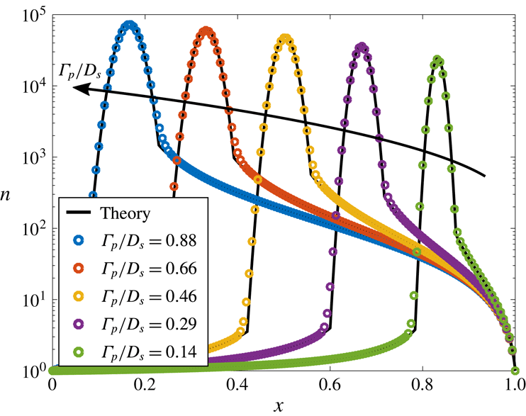
are reported. As can be seen, particles with larger
 $\unicode[STIX]{x1D6E4}_{p}/D_{s}$
experience diffusiophoresis more strongly, and are able to propagate further upstream towards the channel inlet. As time progresses, particles continue to focus, and the particle concentrations will continue to grow as described in the previous section. However, after the initial
 $t=O(1)$
period, the locations of the peaks remain effectively stationary.
Suspended particle concentration profiles for particles with different diffusiophoretic mobilities
 $\unicode[STIX]{x1D6E4}_{p}/D_{s}$
for
 $Pe_{s}=0.75$
,
 $D_{p}/D_{s}=6.25\times 10^{-4}$
,
 $\unicode[STIX]{x1D6FD}=0.01$
and
 $t=36.0$
. Symbols denote numerical solutions of the 1-D equation (2.1), and solid black lines indicate the corresponding theoretical predictions given by (3.8a
), (3.8b
) and (3.11). As can be seen, particles with different diffusiophoretic mobilities form distinct peaks (the locations of which are steady in time), suggesting that this type of system may have significant applications such as particle sorting, focusing and zeta potentiometry.
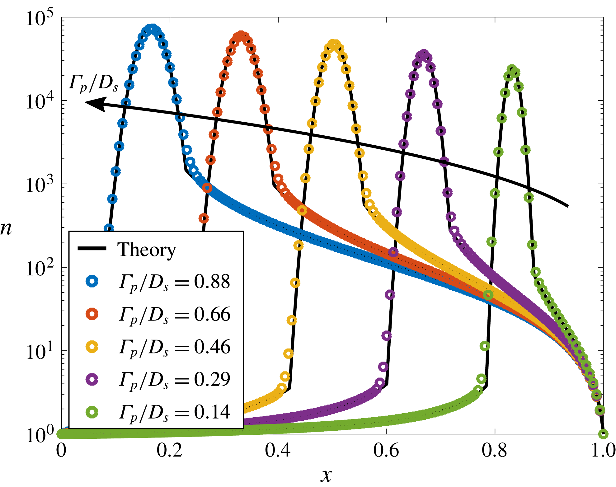
Another way to interpret the results of figure 5 is to consider a channel simultaneously filled with a uniform dilute concentration of five different types of particles with the values of
 $\unicode[STIX]{x1D6E4}_{p}/D_{s}$
specified in the figure. Due to the combined influences of fluid advection and diffusiophoresis, as time passes, the particle concentrations will begin to focus at different locations in the channel, forming distinct concentration peaks, effectively sorting and focusing each of the particles based on their
 $\unicode[STIX]{x1D6E4}_{p}/D_{s}$
.
This configuration has potential applications ranging from particle sorting, separation and focusing, to diagnostic and measurement applications. For example, since the peak concentration locations are steady in time after an initial transient of time
 $t=O(1)$
, and the locations for accumulation are uniquely determined by the system parameters
 $Pe_{s}$
,
 $\unicode[STIX]{x1D6E4}_{p}/D_{s}$
, and
 $\unicode[STIX]{x1D6FD}$
, it is straightforward to establish the
 $\unicode[STIX]{x1D6E4}_{p}$
of the different particles. For example, in a microfluidic experiment, with fixed
 $\unicode[STIX]{x1D6FD}$
and
 $Pe_{s}$
, the position of the peak concentration
 $x_{p}^{\infty }$
for particles with unknown
 $\unicode[STIX]{x1D6E4}_{p}$
can easily be measured. Then, the unknown diffusiophoretic mobility can be directly calculated from (3.10) to yield
 $$\begin{eqnarray}\unicode[STIX]{x1D6E4}_{p}=D_{s}\left(\frac{\unicode[STIX]{x1D6FD}-\text{e}^{Pe_{s}}}{\text{e}^{Pe_{s}x_{p}^{\infty }}(\unicode[STIX]{x1D6FD}-1)}-1\right).\end{eqnarray}$$
This approach is similar to that described by Shin et al. (Reference Shin, Ault, Feng, Warren and Stone2017a
), who used a dead-end pore geometry. However, the configuration of figure 1 has several advantages. First, the particle concentration peak location is stationary in time, and results can be achieved based only on a single snapshot in time, whereas Shin et al.’s method requires tracking a propagating particle front. Furthermore, the precision of this approach can likely be higher than that described by Shin et al., where, for typical
 $\unicode[STIX]{x1D6E4}_{p}$
, the quasi-steady locations that particle fronts approach only occupy a range covering approximately 30 % of the total channel length, such that in the case of multiple particles, they lie relatively close together in the measurement. Here,
 $Pe_{s}$
and
 $\unicode[STIX]{x1D6FD}$
can be tuned to maximize separation between particles and improve measurement resolution. Finally, our proposed approach has a straightforward analytical expression given by (4.1) that can be used to calculate
 $\unicode[STIX]{x1D6E4}_{p}$
.
Furthermore, we note that in the thin double layer limit the diffusiophoretic mobility
 $\unicode[STIX]{x1D6E4}_{p}$
is a known function of both a particle’s surface charge (i.e. zeta potential) and size. Shin et al. also took advantage of this size effect, demonstrating particle separation by size using applied transient solute gradients (Shin et al.
Reference Shin, Um, Sabass, Ault, Rahimi, Warren and Stone2016). For much the same reasons as stated above, the system presented here again offers additional advantages over Shin et al.’s system, specifically (i) particle peak locations are steady in time, (ii) the system undergoes steady, continuous particle focusing and accumulation in contrast to transient, limited focusing and (iii) convenient analytical expressions exist that relate
 $\unicode[STIX]{x1D6E4}_{p}/D_{s}$
,
 $Pe_{s}$
,
 $\unicode[STIX]{x1D6FD}$
and the steady-state particle peak location
 $x_{p}^{\infty }$
. As illustrated in figure 5, the flow configuration of figure 1 provides a simple, practical means to predictably manipulate particles by size and/or surface charge in long narrow channels. In the next section, we will look at two-dimensional corrections to the fluid, solute and particle dynamics due to the finite aspect ratio of channels, and especially consider the effects of diffusioosmosis at the channel walls.
5 Diffusiophoresis in 2-D narrow channel flows
In § 3, we used an asymptotic expansion with the small parameter
 $\unicode[STIX]{x1D716}=h/L\ll 1$
to solve for the leading-order, quasi-1-D solute and particle concentration profiles in a long, narrow channel flow. We showed that the solute and particle concentrations only depend on the mean channel velocity
 $\bar{U}$
(through the solute Péclet number
 $Pe_{s}$
) and are independent of the distribution of velocity
 $\boldsymbol{u}(x,y,t)$
to leading order, i.e. the influence of diffusioosmosis on the solute and particle concentrations is negligible to leading order. Thus, the leading-order 1-D analysis fails to model the effects of both finite-aspect-ratio channels and the recirculating flows due to diffusioosmotic wall slip conditions. In this section, we extend the analysis of § 3 to higher order to include the effects of diffusioosmosis and provide 2-D corrections to the solute/particle dynamics for finite
 $\unicode[STIX]{x1D716}$
. Thus, in this section we quantify the influence of diffusioosmosis expressed through the diffusioosmotic mobility coefficient
 $\unicode[STIX]{x1D6E4}_{w}$
which is a function of, among other things, the surface charge density of the channel walls. First, we solve for the leading-order 2-D fluid velocity and pressure distributions, which are needed to develop the higher-order corrections to the solute and particle concentration profiles. Next, we calculate the higher-order 2-D correction to the solute concentration profile and use this result to determine the particle velocity components
 $u_{p}$
and
 $v_{p}$
due to both fluid advection and diffusiophoresis up to
 $O(\unicode[STIX]{x1D716}^{2})$
, which can be directly integrated to yield individual particle trajectories. Finally, we calculate the 2-D correction to the particle concentration around the peak for finite
 $\unicode[STIX]{x1D716}$
and show that the particles form a curved band depending on the strength of the diffusioosmotic effects.
5.1 Leading-order base flow
In § 3 we showed that the leading-order fluid velocity and pressure profiles are governed by (3.2), although only the mean velocity
 $\bar{U}$
influenced the leading-order distribution of solute (
 $c_{0}$
) and particles (
 $n_{0}$
). In order to solve for the higher-order 2-D corrections to the solute/particle dynamics, we next seek solutions to the fluid velocity,
 $\boldsymbol{u}_{0}=(u_{0},v_{0})$
, and pressure profiles. Subject to the leading-order boundary conditions
 $$\begin{eqnarray}\int _{0}^{1}u_{0}(x,y)\,\text{d}y=1\quad \text{and}\quad u_{0}(x,\pm 1)=-\frac{\unicode[STIX]{x1D6E4}_{w}}{L\bar{U}}\,\frac{\text{d}\ln c_{0}}{\text{d}x},\end{eqnarray}$$
the solution to (3.2) is given by
 $$\begin{eqnarray}\displaystyle & \displaystyle u_{0}(x,y)=\frac{1}{2}\left[3-3y^{2}-\frac{\unicode[STIX]{x1D6E4}_{w}}{D_{s}}\left(\frac{\text{e}^{Pe_{s}x}(3y^{2}-1)(\unicode[STIX]{x1D6FD}-1)}{\text{e}^{Pe_{s}}+\text{e}^{Pe_{s}x}(\unicode[STIX]{x1D6FD}-1)-\unicode[STIX]{x1D6FD}}\right)\right], & \displaystyle\end{eqnarray}$$
 $$\begin{eqnarray}\displaystyle & \displaystyle v_{0}(x,y)=Pe_{s}\frac{\unicode[STIX]{x1D6E4}_{w}}{D_{s}}\left[\frac{\text{e}^{Pe_{s}x}(y^{3}-y)(\text{e}^{Pe_{s}}-\unicode[STIX]{x1D6FD})(\unicode[STIX]{x1D6FD}-1)}{2(\text{e}^{Pe_{s}}+\text{e}^{Pe_{s}x}(\unicode[STIX]{x1D6FD}-1)-\unicode[STIX]{x1D6FD})^{2}}\right], & \displaystyle\end{eqnarray}$$
 $$\begin{eqnarray}\displaystyle & \displaystyle p_{0}(x)=3\left[1-x+\frac{\unicode[STIX]{x1D6E4}_{w}}{L\bar{U}}(\ln [(\text{e}^{Pe_{s}}-1)\unicode[STIX]{x1D6FD}]-\ln [\text{e}^{Pe_{s}}+\text{e}^{Pe_{s}x}(\unicode[STIX]{x1D6FD}-1)-\unicode[STIX]{x1D6FD}])\right]. & \displaystyle\end{eqnarray}$$
 $t=O(1)$
, which is the time scale for the solute concentration to approach steady state. Note that diffusiophoresis typically occurs in aqueous solutions for which
 $\unicode[STIX]{x1D708}\gg D_{s}$
and the flows have
 $Re\ll 1$
, so that the fluid velocity and pressure profiles adjust nearly instantaneously relative to the solute dynamics.
As validation of these results, we choose
 $Pe_{s}=10$
,
 $\unicode[STIX]{x1D716}=0.0025$
,
 $\unicode[STIX]{x1D6FD}=0.01$
and
 $\unicode[STIX]{x1D6E4}_{w}/L\bar{U}=0.1$
and compare the theoretical predictions for the fluid velocity components given by (5.2a
) and (5.2b
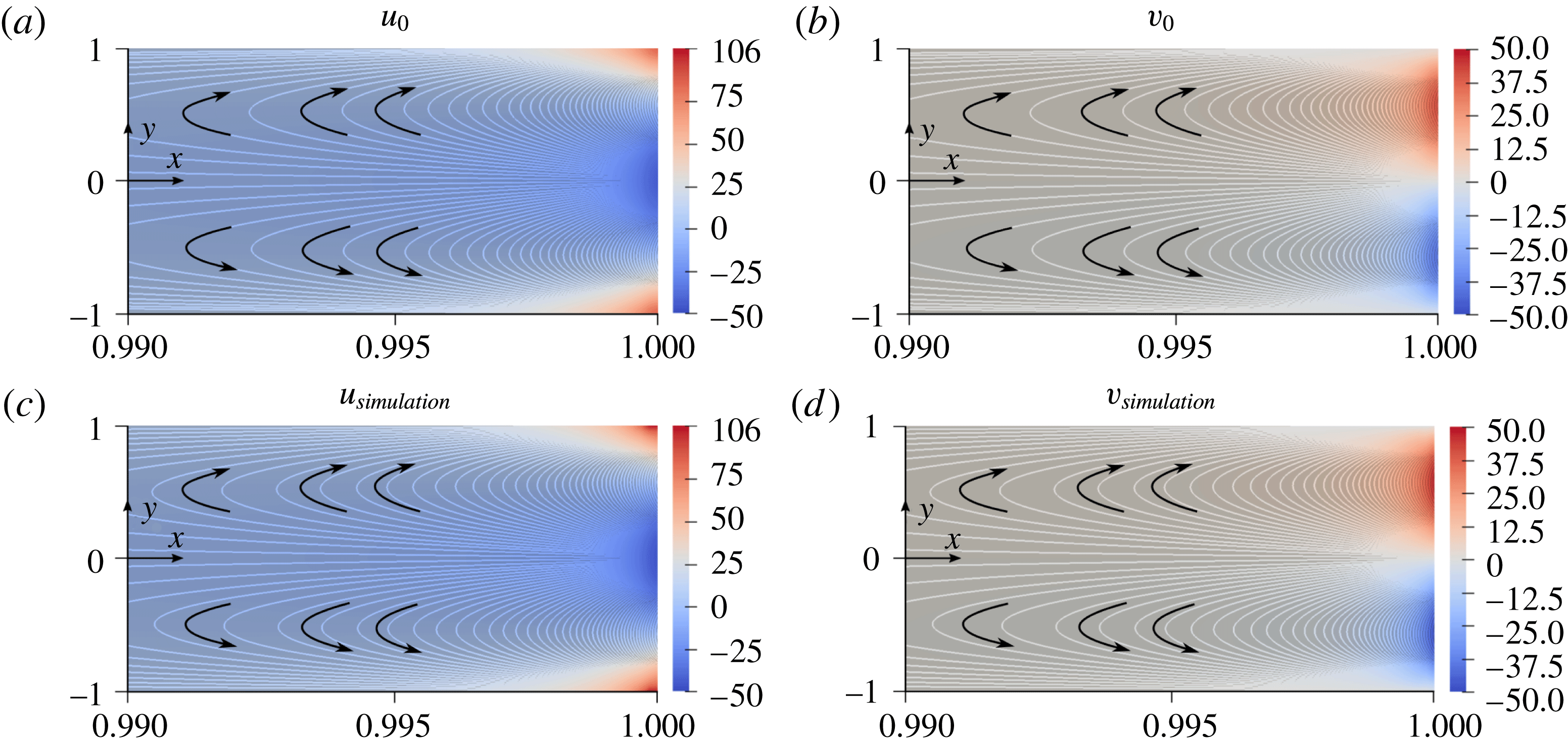
) with the results of 2-D numerical simulations of (2.1) in figure 6. Details of the numerical simulations are given in appendix A. We restrict the figure to the region of the channel near the outlet (
 $0.99\leqslant x\leqslant 1.0$
) because that corresponds to the region with the largest deviations from the parabolic Poiseuille flow for the chosen parameters. As can be seen, for
 $\unicode[STIX]{x1D6E4}_{w}>0$
diffusioosmosis drives an outflow slip boundary condition at the channel walls at the outlet, which can lead to a flow reversal along the channel centreline for sufficiently charged channel walls. This flow reversal in turn drives a recirculating flow, as seen in figure 6(b,d), which drives flow towards the channel walls.
Steady-state fluid velocity components near the outlet (
 $x=1$
). The four panels indicate the theoretical prediction for (a) the leading-order
 $x$
-component of velocity
 $u_{0}$
and (b) the leading-order
 $y$
-component of velocity
 $v_{0}$
, as well as the results of numerical simulations for
 $u$
and
 $v$
in (c) and (d), respectively. Results correspond to
 $\unicode[STIX]{x1D6FD}=0.01$
,
 $\unicode[STIX]{x1D716}=h/L=0.0025$
,
 $Pe_{s}=10$
and
 $\unicode[STIX]{x1D6E4}_{w}/L\bar{U}=0.1$
. Theoretical predictions are given by (5.2a
) and (5.2b
). In the vicinity of the channel outlet, diffusioosmosis at the channel walls results in a slip boundary condition towards the outlet. If this diffusioosmosis is strong enough, conservation of mass requires that some fluid is pulled into the domain along the centreline of the outlet, resulting in a recirculating flow that can drive suspended particles outwards toward the channel walls.
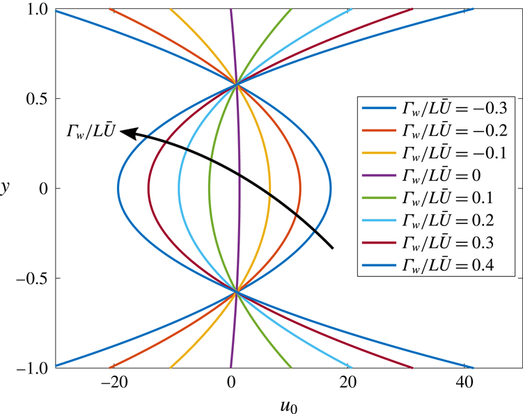
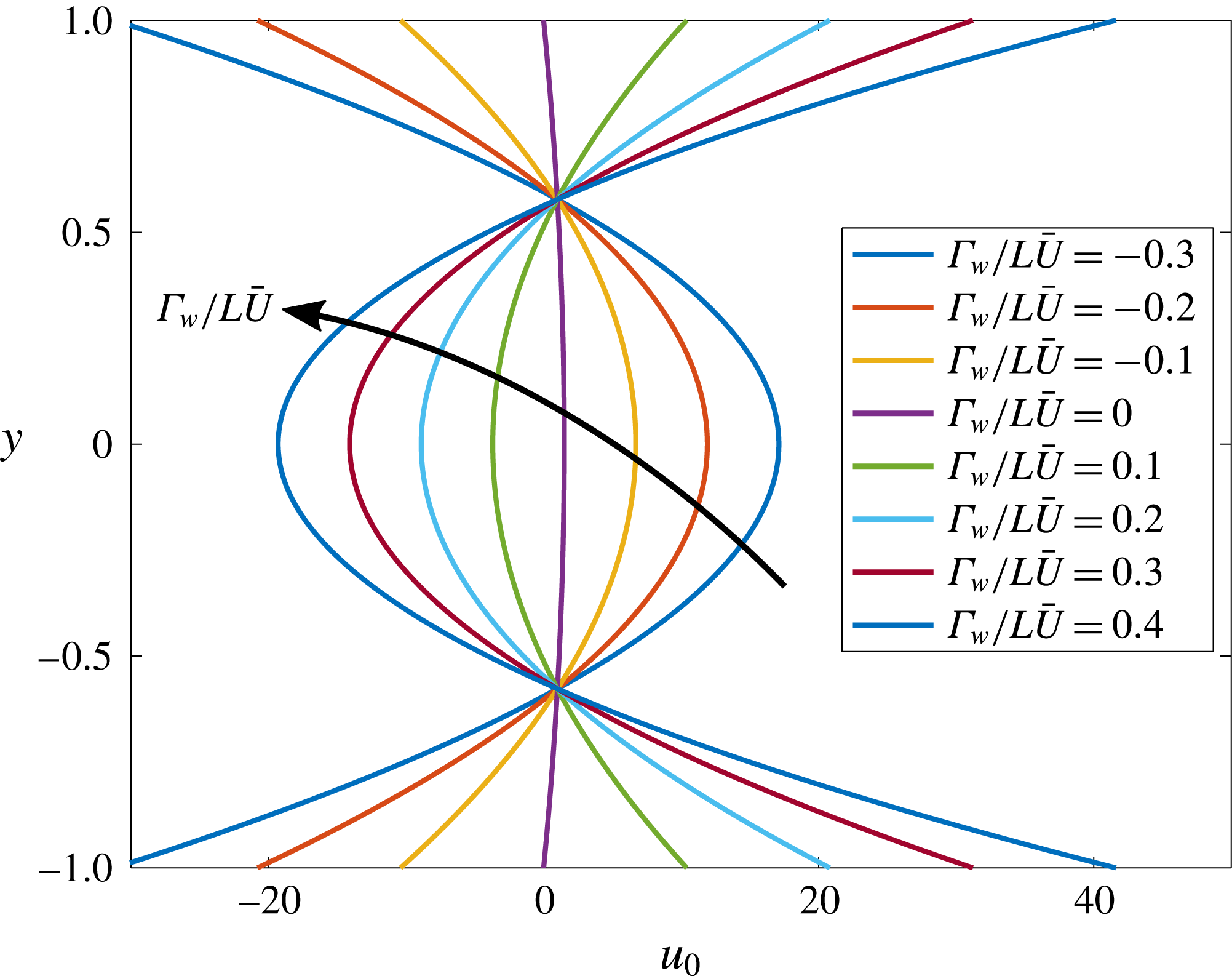
This flow reversal is seen more clearly as a function of the wall surface charge
 $\unicode[STIX]{x1D6E4}_{w}/L\bar{U}$
in figure 7. Increasing the value of
 $\unicode[STIX]{x1D6E4}_{w}/L\bar{U}$
above 0 leads to stronger outflow at the channel walls at the outlet, in turn driving
 $u$
negative along the channel centreline in order to conserve mass. In contrast, decreasing the value of
 $\unicode[STIX]{x1D6E4}_{w}/L\bar{U}$
below 0 leads to an inflow wall slip condition at the channel walls at the outlet, driving a larger outflow velocity along the channel centreline. In each case, the net mass outflux at the outlet is identical to that of parabolic Poiseuille flow (
 $\unicode[STIX]{x1D6E4}_{w}/L\bar{U}=0$
), although the pressure gradient at the outlet will deviate from that of Poiseuille flow as predicted by (5.2c
) for non-zero
 $\unicode[STIX]{x1D6E4}_{w}/L\bar{U}$
.
Influence of diffusioosmosis on the leading-order velocity profile
 $u_{0}$
at the channel outlet (
 $x=1$
). With
 $\unicode[STIX]{x1D6E4}_{w}/L\bar{U}=0$
, the flow satisfies the no-slip condition
 $u_{0}=0$
at the channel walls. However, with
 $\unicode[STIX]{x1D6E4}_{w}/L\bar{U}<0$
, fluid inflow occurs at the channel walls, and with
 $\unicode[STIX]{x1D6E4}_{w}/L\bar{U}>0$
, fluid outflow occurs at the channel walls. All curves integrate to the same net mass flux in order to conserve mass along the channel, although the different profiles correspond to different total pressure drops along the pore.
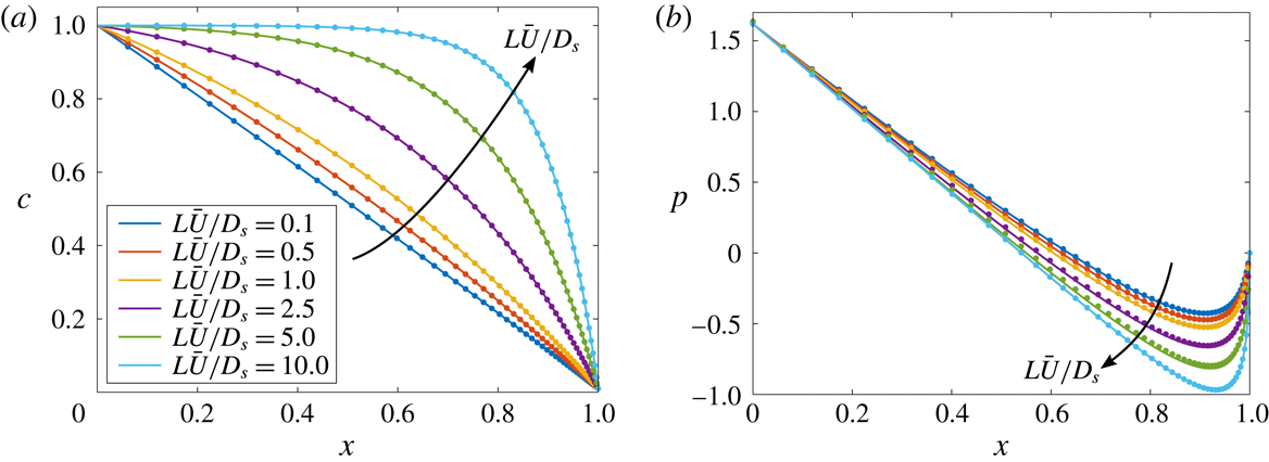
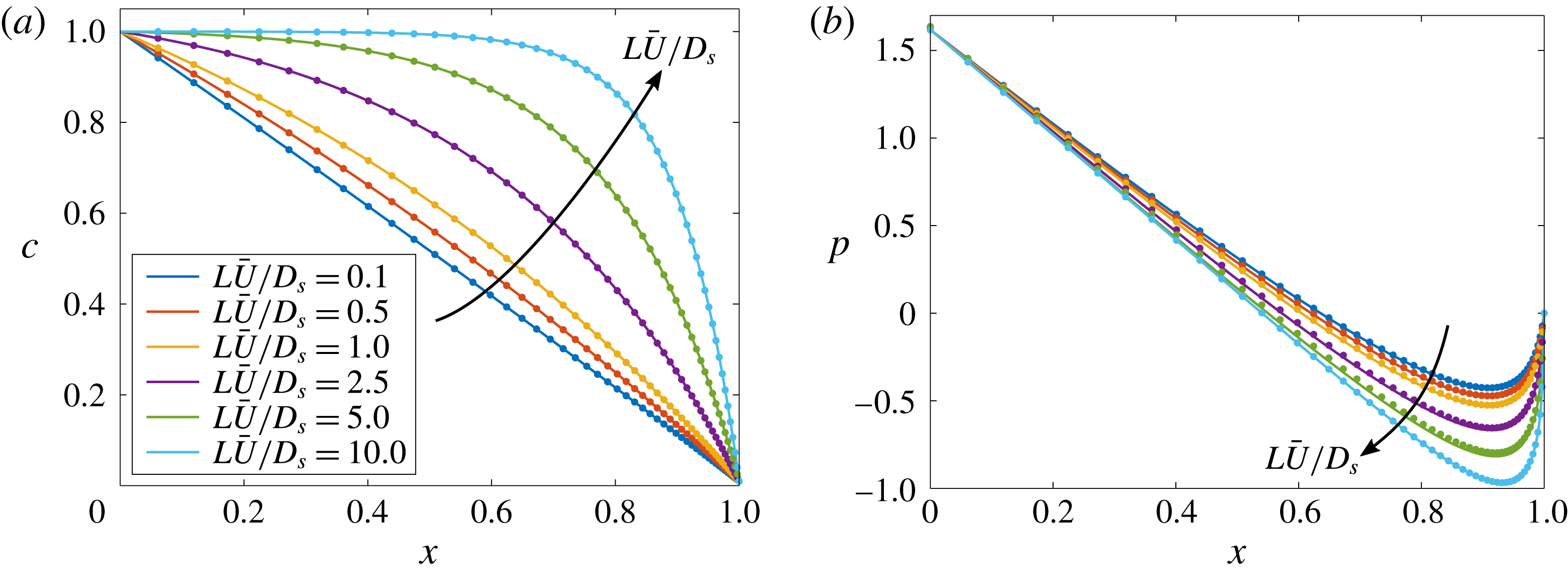
Finally, the theoretical predictions for the leading-order solute concentration and fluid pressure profiles
 $c_{0}$
and
 $p_{0}$
given by (3.6) and (5.2c
) are compared with the results of 2-D numerical simulations in figure 8. As can be seen, increasing the solute Péclet number leads to steeper gradients in both the fluid pressure and solute concentration. Increasing
 $Pe_{s}=L\bar{U}/D_{s}$
increases the relative influence of advection to solute diffusion, extending a region of roughly uniform solute concentration from the inlet, and confining the diffusive region towards the outlet. The steeper solute concentration gradients near the outlet in turn drive stronger diffusioosmosis at the channel walls. In figure 8,
 $\unicode[STIX]{x1D6E4}_{w}/L\bar{U}=0.1$
, thus the wall slip velocity is directed towards the outlet, which leads to a flow reversal on the centreline. This in turn requires a steeper pressure gradient at the outlet in order to maintain the same flow rate. The pressure and solute concentration gradients in the boundary layer near the outlet are given by
 $$\begin{eqnarray}\frac{\text{d}p_{0}}{\text{d}x}=3\left(\frac{\unicode[STIX]{x1D6E4}_{w}}{D_{s}}\frac{\text{e}^{Pe_{s}}(1-\unicode[STIX]{x1D6FD})}{(\text{e}^{Pe_{s}}-1)\unicode[STIX]{x1D6FD}}-1\right)\quad \text{and}\quad \frac{\text{d}c_{0}}{\text{d}x}=Pe_{s}\frac{\text{e}^{Pe_{s}}(\unicode[STIX]{x1D6FD}-1)}{\text{e}^{Pe_{s}}-1}\quad \text{at }x=1.\end{eqnarray}$$
Thus, the pressure gradient at the outlet scales linearly with
 $\unicode[STIX]{x1D6E4}_{w}/D_{s}$
, and the solute concentration gradient at the outlet is proportional to
 $Pe_{s}$
.
Steady-state results for the leading-order (a) solute concentration
 $c_{0}$
and (b) pressure
 $p_{0}$
for
 $\unicode[STIX]{x1D6FD}=0.01$
,
 $\unicode[STIX]{x1D716}=0.0025$
and
 $\unicode[STIX]{x1D6E4}_{w}/L\bar{U}=0.1$
. Solid lines represent the theoretical predictions given by (3.6) and (5.2c
), and symbols represent results from 2-D simulations of the original governing (2.1). Increasing the value of
 $Pe_{s}=L\bar{U}/D_{s}$
increases the relative importance of fluid advection compared to solute diffusion, leading to steeper solute concentration gradients near the outlet. This steeper gradient drives a stronger diffusioosmotic wall slip condition near the outlet, resulting in a stronger adverse pressure gradient at the outlet.
5.2 Two-dimensional solute dynamics
With leading-order relationships for the 2-D base flow in long, narrow channels including diffusioosmotic effects, we now seek the higher-order 2-D correction to the solute concentration profile. Substituting
 $u_{0}$
,
 $v_{0}$
and
 $c_{0}$
into the series expansions (3.1) and considering times
 $t>O(1)$
such that
 $u$
,
 $v$
and
 $c$
can all be assumed steady, equation (2.3d
) leads to
 $$\begin{eqnarray}\frac{\unicode[STIX]{x2202}^{2}c_{1}}{\unicode[STIX]{x2202}y^{2}}=\frac{\displaystyle \text{e}^{Pe_{s}x}Pe_{s}^{2}(3y^{2}-1)\left[(\text{e}^{Pe_{s}}-\unicode[STIX]{x1D6FD})+\text{e}^{Pe_{s}x}(\unicode[STIX]{x1D6FD}-1)\left(1+\frac{\unicode[STIX]{x1D6E4}_{w}}{D_{s}}\right)\right]}{2(\text{e}^{Pe_{s}}-1)(\text{e}^{Pe_{s}}+\text{e}^{Pe_{s}x}(\unicode[STIX]{x1D6FD}-1)-\unicode[STIX]{x1D6FD})(1-\unicode[STIX]{x1D6FD})^{-1}},\end{eqnarray}$$
which has the solution
 $$\begin{eqnarray}c_{1}(x,y)=Pe_{s}^{2}\frac{\displaystyle \text{e}^{Pe_{s}x}y^{2}(y^{2}-2)\left(\text{e}^{Pe_{s}}+\text{e}^{Pe_{s}x}\left(1+\frac{\unicode[STIX]{x1D6E4}_{w}}{D_{s}}\right)(\unicode[STIX]{x1D6FD}-1)-\unicode[STIX]{x1D6FD}\right)}{8(\text{e}^{Pe_{s}}-1)(\text{e}^{Pe_{s}}+\text{e}^{Pe_{s}x}(\unicode[STIX]{x1D6FD}-1)-\unicode[STIX]{x1D6FD})(1-\unicode[STIX]{x1D6FD})^{-1}}+F_{2}(x),\end{eqnarray}$$
where
 $F_{2}(x)$
is an unknown function of
 $x$
that may be determined by extending the analysis to higher order and applying the boundary conditions. Fortunately, the leading-order 2-D particle trajectories can be calculated without an explicit relation for
 $F_{2}(x)$
since
 $\unicode[STIX]{x2202}c_{1}/\unicode[STIX]{x2202}y$
is known explicitly. In the next section, we calculate the leading-order 2-D particle velocity components due to both fluid advection and diffusiophoresis, and we use these to calculate the 2-D particle concentration dynamics for finite
 $\unicode[STIX]{x1D716}$
.
5.3 Two-dimensional particle dynamics
In this section, we extend the results of the previous sections to calculate the leading-order 2-D correction to the diffusiophoretic particle dynamics governed by (2.3e
) for finite
 $\unicode[STIX]{x1D716}$
. With the analytical form for
 $c_{1}$
given by (5.5) in the previous section, individual particle velocities can be directly computed to leading order using
 $$\begin{eqnarray}\displaystyle & \displaystyle u_{p}=u+\frac{\unicode[STIX]{x1D6E4}_{p}}{L\bar{U}}\frac{\unicode[STIX]{x2202}\ln c}{\unicode[STIX]{x2202}x}=u_{0}+\frac{\unicode[STIX]{x1D6E4}_{p}}{L\bar{U}}\,\frac{\text{d}\ln c_{0}}{\text{d}x}+O(\unicode[STIX]{x1D716}^{2}), & \displaystyle\end{eqnarray}$$
 $$\begin{eqnarray}\displaystyle & \displaystyle v_{p}=v+\frac{1}{\unicode[STIX]{x1D716}^{2}}\frac{\unicode[STIX]{x1D6E4}_{p}}{L\bar{U}}\frac{\unicode[STIX]{x2202}\ln c}{\unicode[STIX]{x2202}y}=v_{0}+\frac{\unicode[STIX]{x1D6E4}_{p}}{L\bar{U}}\frac{\unicode[STIX]{x2202}\ln c_{1}}{\unicode[STIX]{x2202}y}+O(\unicode[STIX]{x1D716}^{2}). & \displaystyle\end{eqnarray}$$
 $u_{0}$
,
 $v_{0}$
,
 $c_{0}$
and
 $c_{1}$
, the particle velocity components are given by
 $$\begin{eqnarray}\displaystyle & & \displaystyle u_{p}(x,y)=\nonumber\\ \displaystyle & & \displaystyle \quad \frac{\displaystyle 3(1-y^{2})(\text{e}^{Pe_{s}}-\unicode[STIX]{x1D6FD})+\text{e}^{Pe_{s}x}\left[3+\frac{2\unicode[STIX]{x1D6E4}_{p}+\unicode[STIX]{x1D6E4}_{w}}{D_{s}}-3\left(1+\frac{\unicode[STIX]{x1D6E4}_{w}}{D_{s}}\right)y^{2}\right](\unicode[STIX]{x1D6FD}-1)}{2(\text{e}^{Pe_{s}}+\text{e}^{Pe_{s}x}(\unicode[STIX]{x1D6FD}-1)-\unicode[STIX]{x1D6FD})}+O(\unicode[STIX]{x1D716}^{2}),\nonumber\\ \displaystyle & & \displaystyle\end{eqnarray}$$
 $$\begin{eqnarray}\displaystyle & & \displaystyle v_{p}(x,y)=\nonumber\\ \displaystyle & & \displaystyle \quad \frac{\displaystyle Pe_{s}\text{e}^{Pe_{s}x}(y^{3}-y)\left[\frac{\unicode[STIX]{x1D6E4}_{w}-\unicode[STIX]{x1D6E4}_{p}}{D_{s}}(\text{e}^{Pe_{s}}-\unicode[STIX]{x1D6FD})-\text{e}^{Pe_{s}x}\frac{\unicode[STIX]{x1D6E4}_{p}}{D_{s}}\left(1+\frac{\unicode[STIX]{x1D6E4}_{w}}{D_{s}}\right)(\unicode[STIX]{x1D6FD}-1)\right]}{2(\text{e}^{Pe_{s}}+\text{e}^{Pe_{s}x}(\unicode[STIX]{x1D6FD}-1)-\unicode[STIX]{x1D6FD})^{2}(\unicode[STIX]{x1D6FD}-1)^{-1}}+O(\unicode[STIX]{x1D716}^{2}).\nonumber\\ \displaystyle & & \displaystyle\end{eqnarray}$$
 $$\begin{eqnarray}y=\pm \left[\frac{\displaystyle 3(\text{e}^{Pe_{s}}-\unicode[STIX]{x1D6FD})+\text{e}^{Pe_{s}x}(\unicode[STIX]{x1D6FD}-1)\left(3+2\frac{\unicode[STIX]{x1D6E4}_{p}}{D_{s}}+\frac{\unicode[STIX]{x1D6E4}_{w}}{D_{s}}\right)}{\displaystyle 3(\text{e}^{Pe_{s}}-\unicode[STIX]{x1D6FD})+3\text{e}^{Pe_{s}x}(\unicode[STIX]{x1D6FD}-1)\left(1+\frac{\unicode[STIX]{x1D6E4}_{w}}{D_{s}}\right)}\right]^{1/2},\end{eqnarray}$$
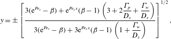
which indicates a locus for particle accumulation.
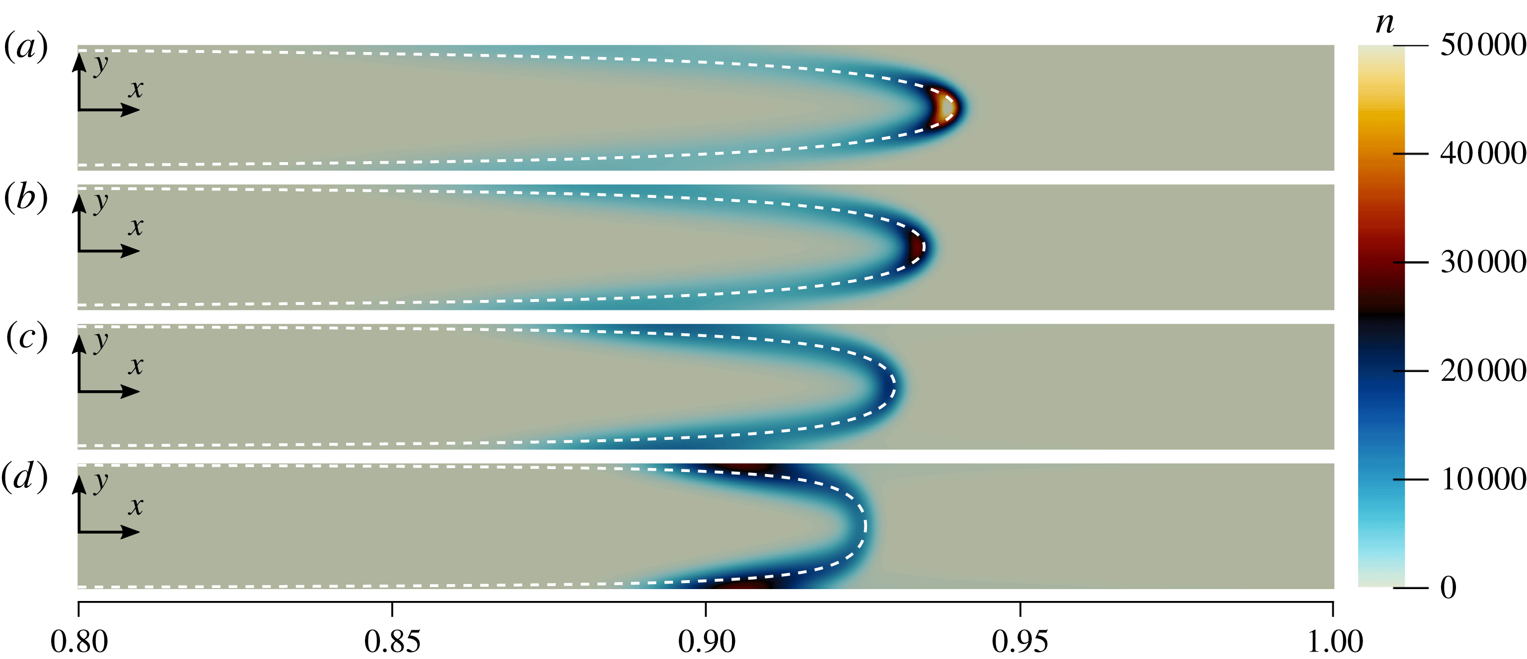
Numerical simulations demonstrating the influence of diffusioosmosis on the suspended particle concentration
 $n$
are shown in figure 9. Here, we clearly see the importance of 2-D effects on the particle dynamics, as
 $n$
forms a curved band for finite
 $\unicode[STIX]{x1D716}$
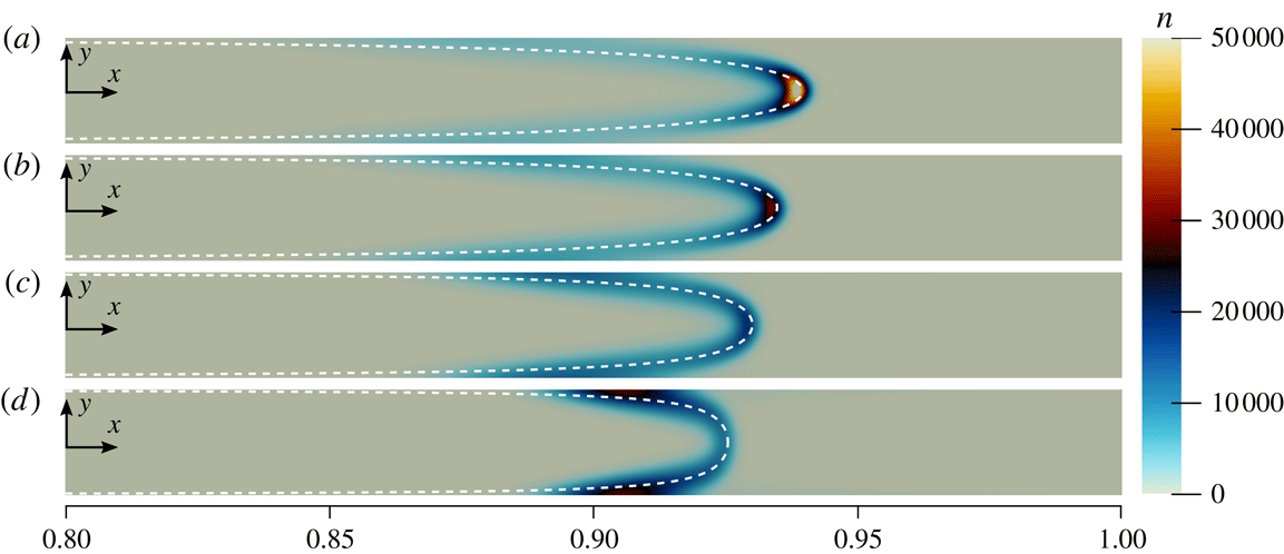
. Figure 9(a) corresponds to the case with the weakest diffusioosmosis at the channel walls. The peak particle concentration forms along the channel centreline near the front of the curved band. Since the fluid velocity is approximately parabolic (due to weak diffusioosmosis in that case), the fluid velocity is fastest along the centreline, leading to the fastest particle accumulation at that point. However, increasing the value of
 $\unicode[STIX]{x1D6E4}_{w}/L\bar{U}$
reduces the fluid velocity along the centreline, increases the magnitude of the wall slip velocity and drives a recirculating flow towards the channel walls. These combined effects drive particles to accumulate closer to the walls for larger
 $\unicode[STIX]{x1D6E4}_{w}/L\bar{U}$
, as shown in figure 9(b–d). The dashed white lines in the figure correspond to the theoretical predictions of (5.8) and correspond to the locations where
 $u_{p}=0$
.
Influence of diffusioosmosis on suspended particle concentrations. Results based on numerical simulations of (2.1) are shown for
 $Pe_{s}=5.0$
,
 $\unicode[STIX]{x1D6FD}=0.01$
,
 $\unicode[STIX]{x1D716}=0.01$
,
 $\unicode[STIX]{x1D6E4}_{p}/D_{s}=0.5$
,
 $D_{p}/D_{s}=0.00025$
and
 $t=1.0$
for (a)
 $\unicode[STIX]{x1D6E4}_{w}/L\bar{U}=0.02$
, (b)
 $\unicode[STIX]{x1D6E4}_{w}/L\bar{U}=0.04$
, (c)
 $\unicode[STIX]{x1D6E4}_{w}/L\bar{U}=0.06$
and (d)
 $\unicode[STIX]{x1D6E4}_{w}/L\bar{U}=0.08$
. Increasing the value of
 $\unicode[STIX]{x1D6E4}_{w}/L\bar{U}$
increases the outflow velocity boundary condition at the walls near the outlet. Due to mass conservation, this reduces the centreline outflow velocity (even reversing the centreline flow to inflow for strong enough diffusioosmosis), leading to a shift of particle concentrations toward the inlet. The diffusioosmosis also sets up a recirculating flow that drives particles toward the channel walls. Dashed white lines correspond to the theoretical prediction of zero axial particle velocity given by (5.8).
Before proceeding to calculate the two-dimensional
 $O(\unicode[STIX]{x1D716}^{2})$
correction to the suspended particle concentration
 $n$
, we first confirm that the results of 2-D numerical simulations do in fact approach the quasi-1-D results of § 3 as
 $\unicode[STIX]{x1D716}\rightarrow 0$
. First, note that the numerical results in figure 9 clearly display 2-D behaviour, although
 $\unicode[STIX]{x1D716}$
has a relatively small value of 0.01. Indeed, the corresponding solute concentration profiles in those cases are approximately one-dimensional. Examining the governing equations given by (2.3) clarifies this apparent contradiction. Equation (2.3d
) shows that the solute concentration profile will be approximately one-dimensional for
 $\unicode[STIX]{x1D716}^{2}\ll 1$
and
 $Pe_{s}\unicode[STIX]{x1D716}^{2}\ll 1$
. We have thus far neglected this second condition because we have been considering
 $Pe_{s}=O(1)$
. However, equation (2.3e
) shows that in order for the particle concentration to be approximately one-dimensional, we must also have
 $\unicode[STIX]{x1D716}^{2}(D_{s}/D_{p})\ll 1$
, which is typically a stricter requirement than
 $\unicode[STIX]{x1D716}^{2}\ll 1$
, because
 $(D_{s}/D_{p})=O(10^{3})$
.
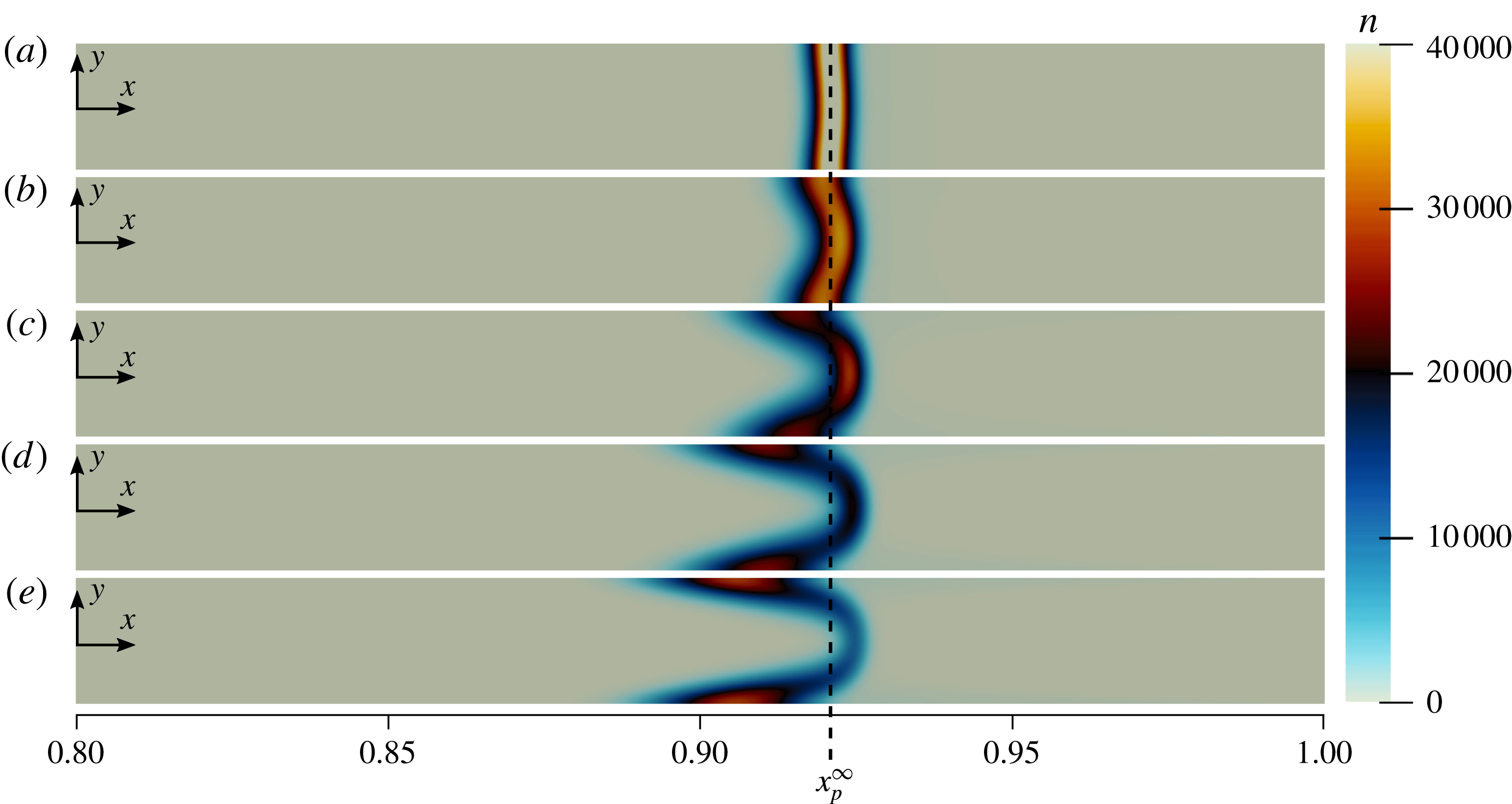
Numerical simulations showing the influence of
 $\unicode[STIX]{x1D716}$
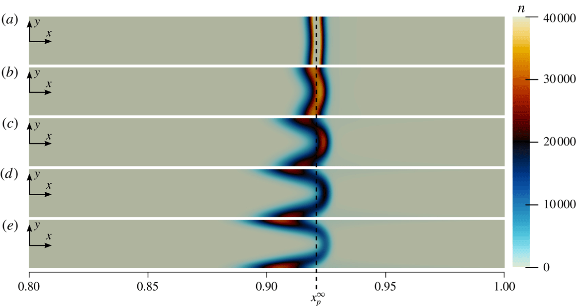
on the suspended particle dynamics are shown in figure 10. As can be seen, 2-D effects decrease as
 $\unicode[STIX]{x1D716}\rightarrow 0$
, and
 $n$
approaches the quasi-1-D results presented in § 3. The corresponding values of
 $\unicode[STIX]{x1D716}^{2}(D_{s}/D_{p})$
for the cases shown in figure 10 are (a) 0.004, (b) 0.025, (c) 0.1, (d) 0.225 and (e) 0.4. These results confirm that for small enough
 $\unicode[STIX]{x1D716}$
, the particle concentrations do in fact approach the quasi-1D results of § 3, although for practical purposes this also requires
 $\unicode[STIX]{x1D716}^{2}(D_{s}/D_{p})\ll 1$
.
Influence of channel aspect ratio
 $\unicode[STIX]{x1D716}$
on suspended particle dynamics. Results based on numerical simulations of (2.1) show the particle concentrations at
 $t=1$
for
 $Pe_{s}=5.0$
,
 $\unicode[STIX]{x1D6E4}_{w}/L\bar{U}=0.08$
,
 $D_{p}/D_{s}=0.00025$
,
 $\unicode[STIX]{x1D6FD}=0.01$
and
 $\unicode[STIX]{x1D6E4}_{p}/D_{s}=0.5$
, for (a)
 $\unicode[STIX]{x1D716}=0.001$
, (b)
 $\unicode[STIX]{x1D716}=0.0025$
, (c)
 $\unicode[STIX]{x1D716}=0.005$
, (d)
 $\unicode[STIX]{x1D716}=0.0075$
and (e)
 $\unicode[STIX]{x1D716}=0.01$
. For very narrow channels, such as in (a), particle dynamics is quasi-one-dimensional and accurately match the predictions from the 1-D theory. For wider channels, the time scale for particles to diffuse across the channel increases, and the relative influence of the recirculating flow due to 2-D effects increases, shifting peak particle concentrations toward the channel walls. Aspect ratios are not to scale.
Next, with the leading-order predictions for
 $u_{p}$
and
 $v_{p}$
given by (5.7), we seek the
 $O(\unicode[STIX]{x1D716}^{2})$
correction to the particle distribution about the peak. Expanding
 $n$
as in (3.1e
) with
 $n_{0}=n_{c}(x,t)$
given by (3.11), equation (2.3e
) simplifies to an unwieldy ordinary differential equation (ODE) for
 $n_{1}(x,y,t)$
, the solution of which can be written somewhat tersely as
 $$\begin{eqnarray}\displaystyle n_{1}(x,y,t) & = & \displaystyle \frac{f_{3}(x,y)}{f_{4}(x)}\left[f_{5}(x,y,t)+f_{7}(x,y,t)+Pe_{s}^{2}tf_{1}(x)\left(-4f_{2}^{2}\left(1+\frac{\unicode[STIX]{x1D6E4}_{p}}{D_{s}}\right)^{2}f_{1}(x)\right.\right.\nonumber\\ \displaystyle & & \displaystyle +\left.\left.\frac{\unicode[STIX]{x1D6E4}_{p}}{D_{s}}f_{6}(x,y)+f_{2}\left(1+\frac{\unicode[STIX]{x1D6E4}_{p}}{D_{s}}\right)f_{8}(x,y)\right)+f_{9}(x,y,t)\right]+F_{3}(x,t),\end{eqnarray}$$
where the
 $f_{i}$
are given in appendix B, and
 $F_{3}(x,t)$
is an unknown function of
 $x$
and
 $t$
. Thus, as with the calculation of the 2-D correction to the solute concentration profile, we have not fully specified the
 $\unicode[STIX]{x1D716}^{2}$
correction due to the
 $F_{2}(x)$
and
 $F_{3}(x,t)$
terms. Presumably, these may be calculated by extending this analysis to higher order and judiciously applying the boundary conditions. Fortunately, the calculated terms include all of the
 $y$
-dependence, and so for a given
 $x$
, equation (5.9) fully captures the
 $y$
-variation in the suspended particle concentrations to leading order.
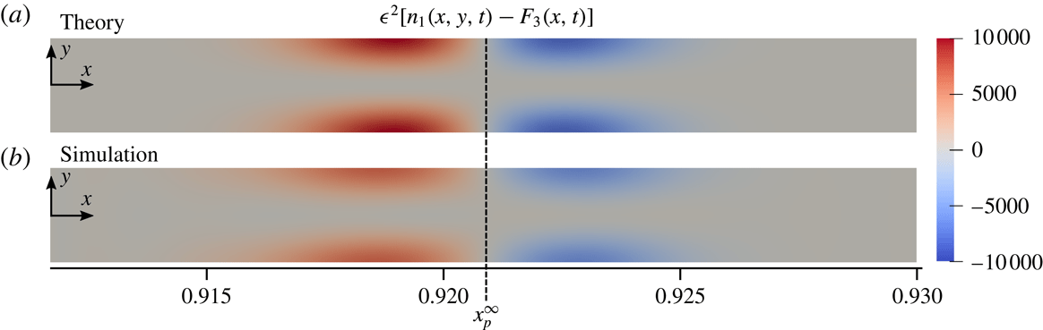
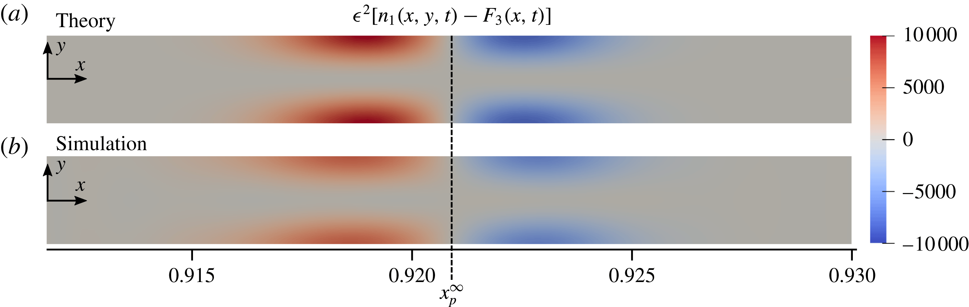
To validate (5.9), we compare the theoretical prediction for
 $n_{1}$
with the results of numerical simulations in figure 11. As can be seen, both qualitative and quantitative agreement between the 2-D numerical simulations and the predictions of (5.9) are good, although the theory predicts slightly larger magnitudes for the 2-D correction. Note that because we do not have an explicit relation for
 $F_{3}(x,t)$
, for the 2-D predictions shown in figure 11, we simply subtracted off the centreline value of
 $n$
from the numerical results in order to produce the figure. The close agreement between theory and numerics supports the validity of our analysis and the use of the formal expansion given by (3.1). However, we briefly note that, as mentioned, the particle concentrations only approach the 1-D results in the limit
 $\unicode[STIX]{x1D716}^{2}\ll D_{p}/D_{s}$
, which is typically a stricter requirement than
 $\unicode[STIX]{x1D716}^{2}\ll 1$
. In the next section, we introduce a phenomenon that we call ‘diffusioosmotic pumping’, which is the diffusioosmotic analogue of electroosmotic flow (EOF) and has applications for pumping fluid against pressure gradients with the use of applied solute concentration gradients.
Comparison between theory and simulations for the leading-order correction to the particle concentration
 $n$
due to 2-D effects. Results are shown at
 $t=1$
for
 $Pe_{s}=5.0$
,
 $\unicode[STIX]{x1D6E4}_{w}/L\bar{U}=0.08$
,
 $D_{p}/D_{s}=0.00025$
,
 $\unicode[STIX]{x1D6FD}=0.01$
and
 $\unicode[STIX]{x1D6E4}_{p}/D_{s}=0.5$
with a channel of aspect ratio
 $\unicode[STIX]{x1D716}=0.001$
. The predicted particle peak position according to the 1-D model is denoted by
 $x_{p}^{\infty }$
. As can be seen, agreement between the theoretical predictions given by (5.9) and the 2-D numerical simulations is qualitatively and quantitatively good, with the theory predicting slightly larger magnitudes for the 2-D correction. While magnitudes increase with
 $t$
, the same qualitative and quantitative agreement holds for long times. For the simulation data we have subtracted the centreline particle concentration from the 2-D particle concentration profile to facilitate direct comparison with
 $\unicode[STIX]{x1D716}^{2}[n_{1}(x,y,t)-F_{3}(x,t)]$
.
6 Diffusioosmotic pumping
In this section, we introduce the idea of diffusioosmotic pumping, which is the consequence of the theory presented in § 5, that is, the use of applied solute gradients to induce diffusioosmotic flows sufficient to pump fluid against an adverse pressure gradient. In characterizing the fluid system presented in figure 1, an intuitive first understanding would suggest that the flow in the pore is due to a pressure-driven flow. However, the derived theoretical solution for the pressure in the pore given by (5.2c
) suggests that this is not always the case. The total pressure drop along the pore
 $\unicode[STIX]{x0394}p=p(1)-p(0)$
is given by
 $$\begin{eqnarray}\unicode[STIX]{x0394}p=-3-3\frac{\unicode[STIX]{x1D6E4}_{w}}{L\bar{U}}\ln \unicode[STIX]{x1D6FD}.\end{eqnarray}$$
Thus, we see that for weakly charged channel walls (
 $|\unicode[STIX]{x1D6E4}_{w}/L\bar{U}|\ll 1$
) we have
 $\unicode[STIX]{x0394}p\approx -3$
which corresponds to typical pressure-driven Poiseuille flow. However, the diffusioosmosis induced by charged channel walls modifies the velocity profiles in the channel, which in turn modifies the pressure gradient along the channel. Thus, by modifying the surface charge of the channel walls through
 $\unicode[STIX]{x1D6E4}_{w}/L\bar{U}$
, we can increase or decrease the pressure gradient necessary to drive the flow. In fact, for channel walls with diffusioosmotic mobilities given by
 $$\begin{eqnarray}\frac{\unicode[STIX]{x1D6E4}_{w}}{L\bar{U}}=-\frac{1}{\ln \unicode[STIX]{x1D6FD}}\end{eqnarray}$$
we will have
 $\unicode[STIX]{x0394}p=0$
, thus no pressure gradient is required to drive the flow, and the diffusioosmosis alone can drive the net fluid motion in the pore. For even more strongly charged channel walls,
 $\unicode[STIX]{x0394}p<0$
, and diffusioosmosis can drive net fluid motion through the pore against a pressure gradient.
This ‘diffusioosmotic pumping’ is shown graphically in figure 12, where we present a variety of pressure profiles in the pore as a function of
 $\unicode[STIX]{x1D6E4}_{w}/L\bar{U}$
. As can be seen, for
 $\unicode[STIX]{x1D6E4}_{w}/L\bar{U}\gtrsim 0.2$
, the inlet pressure actually goes negative, relative to the pressure at the outlet. Thus, we demonstrate theoretically that applied solute gradients can be used to pump fluid against a pressure gradient through the induced fluid motions due to diffusioosmosis. This ‘diffusioosmotic pumping’ is consistent with and analogous to the idea of electrokinetic pumps as described by Kirby (Reference Kirby2010) which consider electroosmotic flows (Manz et al.
Reference Manz, Effenhauser, Burggraf, Harrison, Seiler and Fluri1994) with pressure gradients, except that the driving force here is an applied solute concentration gradient instead of an external electric field. Lee et al. (Reference Lee, Cottin-Bizonne, Biance, Joseph, Bocquet and Ybert2014) achieved an impressive experimental demonstration of flow through fully permeable nanochannels driven by solute gradients and demonstrated unprecedented sensitivity in the measurement of flow rates through the channel. However, they did not solve for the detailed fluid/solute dynamics within the channel, and they appear to have only considered the case
 $\unicode[STIX]{x0394}p=0$
. The results contained herein inform the detailed dynamics in such systems and consider the added complication of diffusiophoretic particle dynamics subject to the background diffusioosmotic flows.
Dependence of pore pressure on the dimensionless diffusioosmotic mobility
 $\unicode[STIX]{x1D6E4}_{w}/L\bar{U}$
of the channel walls for
 $\unicode[STIX]{x1D6FD}=0.01$
and
 $Pe_{s}=0.1$
. With
 $\unicode[STIX]{x1D6E4}_{w}/L\bar{U}=0$
, the pressure forms the expected linear gradient. With
 $\unicode[STIX]{x1D6E4}_{w}/L\bar{U}<0$
, fluid is drawn into the channel along the channel walls at the outlet, which requires a greater inlet pressure to maintain the same flow rate. For
 $\unicode[STIX]{x1D6E4}_{w}/L\bar{U}>0$
, diffusioosmosis causes outflow along the channel walls, reducing the needed inlet pressure to drive the same flow rate. For large enough
 $\unicode[STIX]{x1D6E4}_{w}/L\bar{U}$
, diffusioosmosis can continue to drive the flow even for negative inlet pressures. Thus, diffusioosmosis can be used to pump fluid against a net pressure gradient.
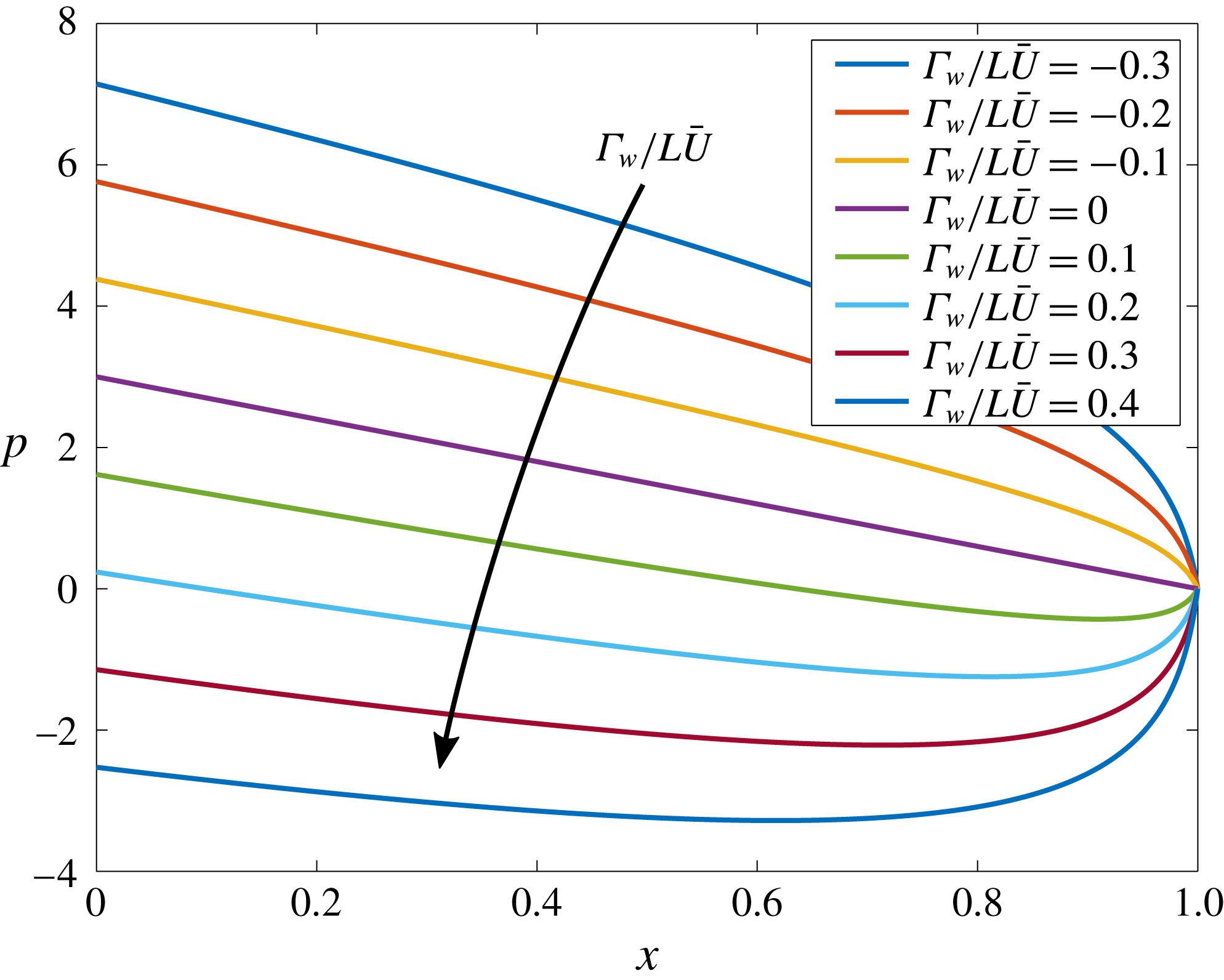
7 Conclusions
In this paper, we have presented a theoretical and numerical analysis of the diffusiophoretic dynamics of suspended charged colloidal particles in narrow channel flows including the effects of diffusioosmotic wall slip conditions. The quasi-1-D model presented in (3.8) and (3.11) provides a theoretical understanding of the rapid particle accumulation documented by Shin et al. (Reference Shin, Ault, Warren and Stone2017b ). Furthermore, the 2-D corrections given by (5.2), (5.5) and (5.9) demonstrate that the preferential particle focusing near the channel walls experimentally seen by Shin et al. (Reference Shin, Ault, Warren and Stone2017b ) is due to diffusioosmotic effects that generate a recirculating flow that drives particles toward the channel walls. The 1-D theory provides an analytical solution for the particle accumulation which includes a peak concentration that grows linearly in time without bound. Of course, particle concentrations can never increase without bound, so that as the particle concentration approaches its maximum packing fraction, short-range interactions and steric effects will dominate and prevent further concentration. Nonetheless, as long as particle–particle and particle–wall interactions are small compared to diffusiophoretic effects, our model describes an approach that can be used to rapidly concentrate particles to high concentrations.
The rate of particle accumulation is described by the proportionality constant
 $k$
(3.12) which is influenced by flow, particle and channel properties. The results demonstrate that the rate of particle accumulation is inversely proportional to the solute concentration ratio
 $\unicode[STIX]{x1D6FD}$
for small
 $\unicode[STIX]{x1D6FD}$
, and directly proportional to
 $Pe_{s}^{2}$
for large
 $Pe_{s}$
. The rate of particle accumulation is also directly proportional to
 $(\unicode[STIX]{x1D6E4}_{p}/D_{p})^{1/2}$
, so increasing the diffusiophoretic mobility of particles relative to the particle diffusivity will also lead to faster particle accumulation. With this understanding, system parameters can be designed to yield specific rates of particle accumulation. Furthermore, with the theoretical description of the particle concentration as a function of time, experimental systems such as that presented in figure 1 can serve as valuable platforms for preconcentrating biological materials, for example, where precise concentrations may be required.
One of the main contributions of this work is the theoretical prediction for the location of the peak particle concentration, which is denoted by
 $x_{p}^{\infty }$
and given by (3.10). The explicit dependence of
 $x_{p}^{\infty }$
on
 $Pe_{s}$
,
 $\unicode[STIX]{x1D6FD}$
and
 $\unicode[STIX]{x1D6E4}_{p}/D_{s}$
makes it possible to design systems in which particles of known
 $\unicode[STIX]{x1D6E4}_{p}$
can be focused to a desired location along a channel, or, in systems with multiple particles, those particles can be selectively focused at distinguished pre-determined positions. This technique has wide applications for sorting, separating and/or focusing particles by
 $\unicode[STIX]{x1D6E4}_{p}$
. Furthermore, because the particle peak position is a steady, known function of
 $\unicode[STIX]{x1D6E4}_{p}$
, the surface charge of the particles can be directly measured by simply observing the location at which the particles accumulate and calculating
 $\unicode[STIX]{x1D6E4}_{p}$
according to (4.1), which represents a new strategy for zeta potentiometry (see also Shin et al.
Reference Shin, Ault, Feng, Warren and Stone2017a
).
The 2-D analysis presented in § 5 provides analytical solutions for the fluid velocity and pressure, as well as the solute concentration in narrow channel flows with the addition of diffusioosmotic effects. These results were presented in (5.2) and (5.5). Furthermore, solutions for the particle velocity components due to both fluid advection and diffusiophoresis were given in (5.7), and can directly be integrated to yield particle trajectories in a narrow channel flow under the combined influence of advection and diffusiophoresis. A series expansion approach about the small parameter
 $\unicode[STIX]{x1D716}^{2}$
was used to solve for the leading-order 2-D corrections to the solute and particle concentration profiles for finite
 $\unicode[STIX]{x1D716}$
, and numerical simulations were used to validate the theory.
Finally, we presented a 2-D theoretical and numerical analysis of the concept of ‘diffusioosmotic pumping’ that was demonstrated experimentally by Lee et al. (Reference Lee, Cottin-Bizonne, Biance, Joseph, Bocquet and Ybert2014). We demonstrated that in these systems, the diffusioosmosis at the channel walls due to applied solute concentration gradients can be sufficient to pump fluid in the absence of any applied pressure gradient, or even in the presence of an applied adverse pressure gradient. One implication of this result is that this type of flow system could potentially be used to directly measure the surface charge of different channel materials or surface treatments simply by measuring the pressure difference across the inlet and outlet. We leave this application for future work. Throughout this work we have relied on the assumption of constant
 $\unicode[STIX]{x1D6E4}_{p}$
and
 $\unicode[STIX]{x1D6E4}_{w}$
as described in § 2.3. One important direction for future work will be to examine the range of system parameters under which such an assumption is valid. Finally, another valuable direction for potential future work is the extension of these ideas to three-dimensional systems such as narrow cylindrical and rectangular pores. It is likely that a two-dimensional, axisymmetric solution is possible for the case of a cylindrical geometry, but for the case of a rectangular pore we expect that fully 3-D effects are inevitable. Performing simulations for the related flow system in Shin et al. (Reference Shin, Ault, Warren and Stone2017b
), we observed the strongest particle accumulation in the corners, likely due to the extra confinement that the flow feels there. We leave the extension of this analysis to such three-dimensional problems as a topic for future work.
Acknowledgements
This manuscript has been authored by UT-Battelle, LLC under contract no. DE-AC05-00OR22725 with the US Department of Energy. The publisher, by accepting the article for publication, acknowledges that the United States Government retains a non-exclusive, paid-up, irrevocable, world-wide licence to publish or reproduce the published form of this manuscript, or allow others to do so, for United States Government purposes. The Department of Energy will provide public access to these results of federally sponsored research in accordance with the DOE Public Access Plan (http://energy.gov/downloads/doe-public-access-plan). Research sponsored by the Laboratory Directed Research and Development Program of Oak Ridge National Laboratory, managed by UT-Battelle, LLC, for the US Department of Energy.
Appendix A. Numerical simulations
Here, we describe the numerical methods used to perform the one-dimensional and two-dimensional simulations. The incompressible Navier–Stokes equations were solved using a finite-volume solver adapted from both the simpleFoam and scalarTransportFoam solvers of the OpenFOAM library (Weller et al.
Reference Weller, Tabor, Jasak and Fureby1998). These were developed into two solvers: simpleScalarTransportFoam, which iteratively uses the SIMPLE algorithm (see, e.g. Ferziger & Peric Reference Ferziger and Peric2012) and scalarTransportFoam to simultaneously solve for the steady-state fluid velocity, pressure and solute concentration profiles, and diffusiophoresisFoam, which solves a modified advection–diffusion equation to determine the transient particle concentration profiles. Spatial derivatives are second-order accurate, and the temporal scheme is fully implicit and also second-order accurate. For the 1-D simulations, 4000 grid cells were used, and for the 2-D simulations,
 $5\times 10^{4}$
grid cells were used. High-resolution convergence tests were performed for each case to verify convergence. For example, for the 2-D cases, convergence tests were performed with
 $2\times 10^{5}$
grid cells and
 $8\times 10^{5}$
grid cells, and example particle concentrations around the peak for these tests are shown at
 $t=1$
in figure 13. Peak particle concentrations for the case with
 $5\times 10^{4}$
grid cells deviated from those with
 $8\times 10^{5}$
grid cells by less than 0.1 % relative error.
Convergence test results showing the particle concentrations around the peak for simulations with
 $5\times 10^{4}$
,
 $2\times 10^{5}$
and
 $8\times 10^{5}$
grid cells with
 $t=1$
,
 $Pe_{s}=5.0$
,
 $\unicode[STIX]{x1D6E4}_{w}/L\bar{U}=0.08$
,
 $D_{p}/D_{s}=0.00025$
,
 $\unicode[STIX]{x1D6FD}=0.01$
,
 $\unicode[STIX]{x1D6E4}_{p}/D_{s}=0.5$
and
 $\unicode[STIX]{x1D716}=0.001$
.
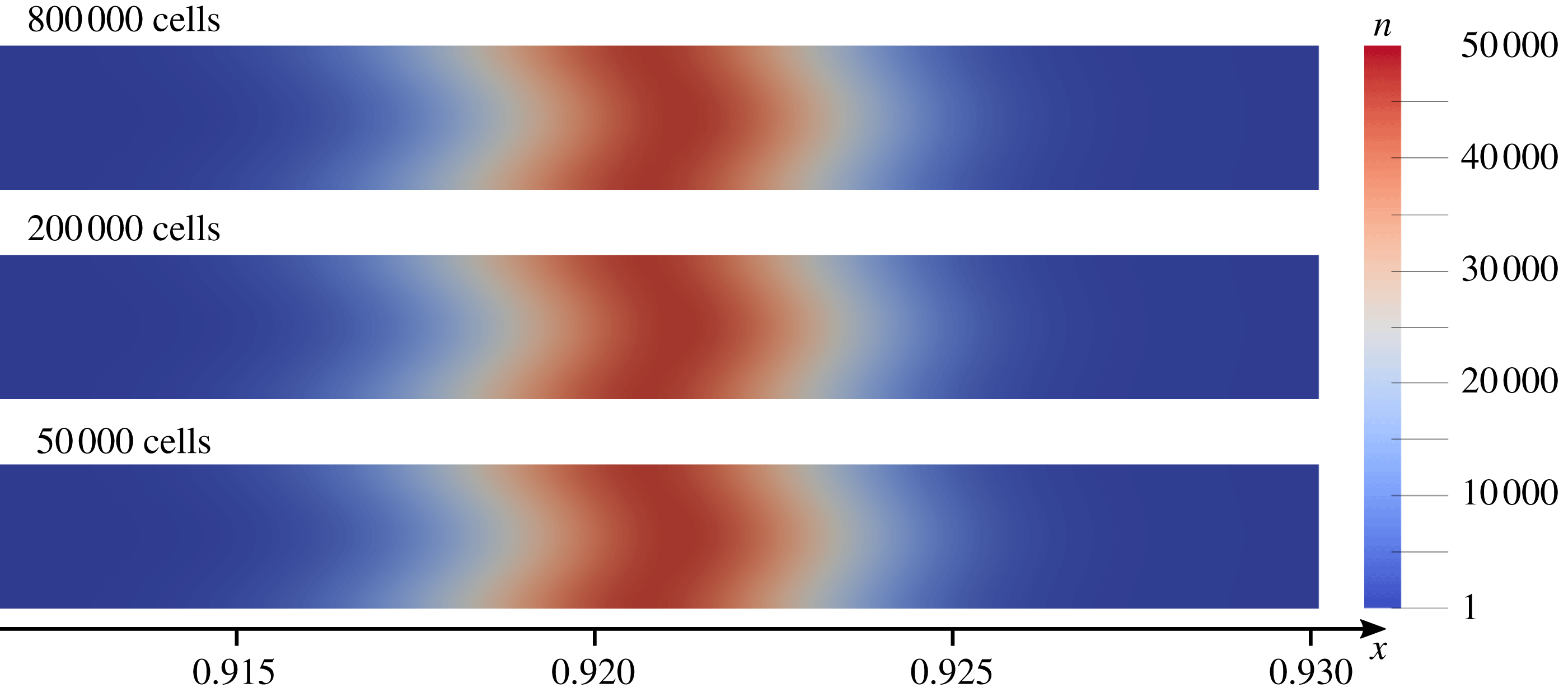
Appendix B. Coefficient functions for 2-D particle corrections
The coefficient functions needed by (5.9) to specify the 2-D correction to the suspended particle concentration are given by
 $$\begin{eqnarray}\displaystyle & \displaystyle f_{1}(x)=\text{e}^{Pe_{s}}+\text{e}^{Pe_{s}x}(\unicode[STIX]{x1D6FD}-1)-\unicode[STIX]{x1D6FD}, & \displaystyle\end{eqnarray}$$
 $$\begin{eqnarray}\displaystyle & \displaystyle f_{2}=\ln \left[\frac{\unicode[STIX]{x1D6FD}-\text{e}^{Pe_{s}}}{\displaystyle (\unicode[STIX]{x1D6FD}-1)\left(1+\frac{\unicode[STIX]{x1D6E4}_{p}}{D_{s}}\right)}\right], & \displaystyle\end{eqnarray}$$
 $$\begin{eqnarray}\displaystyle f_{3}(x,y) & = & \displaystyle Pe_{s}^{2}y^{2}(\text{e}^{Pe_{s}}-\unicode[STIX]{x1D6FD})(1-\unicode[STIX]{x1D6FD})\left[\frac{\unicode[STIX]{x1D6E4}_{p}}{D_{p}}\left(1+\frac{\unicode[STIX]{x1D6E4}_{p}}{D_{s}}\right)\right]^{1/2}\nonumber\\ \displaystyle & & \displaystyle \times \,\exp \left[-\frac{\displaystyle (f_{2}-Pe_{s}x)^{2}\left(1+\frac{\unicode[STIX]{x1D6E4}_{p}}{D_{s}}\right)}{\displaystyle 2\frac{D_{p}}{D_{s}}\frac{\unicode[STIX]{x1D6E4}_{p}}{D_{s}}}\right],\end{eqnarray}$$
 $$\begin{eqnarray}\displaystyle & \displaystyle f_{4}(x)=8\unicode[STIX]{x1D6FD}\sqrt{2\unicode[STIX]{x03C0}}(\text{e}^{Pe_{s}}-1)f_{1}^{2}(x)\left(\frac{D_{p}}{D_{s}}\frac{\unicode[STIX]{x1D6E4}_{p}}{D_{s}}\right)^{2}, & \displaystyle\end{eqnarray}$$
 $$\begin{eqnarray}\displaystyle & \displaystyle f_{5}(x,y,t)=\text{e}^{Pe_{s}x}Pe_{s}^{2}t(1-\unicode[STIX]{x1D6FD})\frac{D_{p}}{D_{s}}\left(\frac{\unicode[STIX]{x1D6E4}_{p}}{D_{s}}\right)^{3}[(y^{2}-6)(\text{e}^{Pe_{s}}-\unicode[STIX]{x1D6FD})+\text{e}^{Pe_{s}x}(y^{2}-2)(\unicode[STIX]{x1D6FD}-1)], & \displaystyle \nonumber\\ \displaystyle & & \displaystyle\end{eqnarray}$$
 $$\begin{eqnarray}\displaystyle f_{6}(x,y) & = & \displaystyle (\text{e}^{Pe_{s}}-\unicode[STIX]{x1D6FD})\left[4\frac{D_{p}}{D_{s}}+Pe_{s}x(y^{2}-4Pe_{s}x-6)\frac{\unicode[STIX]{x1D6E4}_{p}}{D_{s}}\right]\nonumber\\ \displaystyle & & \displaystyle +\,\text{e}^{Pe_{s}x}(\unicode[STIX]{x1D6FD}-1)\left[4\frac{D_{p}}{D_{s}}+Pe_{s}x\left((y^{2}-4Pe_{s}x-10)\frac{\unicode[STIX]{x1D6E4}_{p}}{D_{s}}+(y^{2}-2)\frac{\unicode[STIX]{x1D6E4}_{w}}{D_{s}}\right)\right],\nonumber\\ \displaystyle & & \displaystyle\end{eqnarray}$$
 $$\begin{eqnarray}\displaystyle f_{7}(x,y,t) & = & \displaystyle f_{1}(x)\left(\frac{\unicode[STIX]{x1D6E4}_{p}}{D_{s}}\right)^{2}\left[\text{e}^{Pe_{s}x}Pe_{s}^{3}tx(1-\unicode[STIX]{x1D6FD})\left(4\frac{\unicode[STIX]{x1D6E4}_{p}}{D_{s}}+(2-y^{2})\frac{\unicode[STIX]{x1D6E4}_{w}}{D_{s}}\right)\right.\nonumber\\ \displaystyle & & \displaystyle +\left.4\left(\frac{D_{p}}{D_{s}}+\frac{D_{p}}{D_{s}}Pe_{s}^{2}t\right)f_{1}(x)\right],\end{eqnarray}$$
 $$\begin{eqnarray}\displaystyle f_{8}(x,y) & = & \displaystyle \text{e}^{Pe_{s}x}(\unicode[STIX]{x1D6FD}-1)\frac{\unicode[STIX]{x1D6E4}_{p}}{D_{s}}\left(4\frac{\unicode[STIX]{x1D6E4}_{p}}{D_{s}}+(2-y^{2})\frac{\unicode[STIX]{x1D6E4}_{w}}{D_{s}}\right)+f_{1}(x)\left[(6-y^{2})\frac{\unicode[STIX]{x1D6E4}_{p}}{D_{s}}\right.\nonumber\\ \displaystyle & & \displaystyle +\left.8Pe_{s}x\left(1+\frac{\unicode[STIX]{x1D6E4}_{p}}{D_{s}}\right)\right],\end{eqnarray}$$
 $$\begin{eqnarray}\displaystyle f_{9}(x,y,t) & = & \displaystyle Pe_{s}^{2}t\left[\text{e}^{2Pe_{s}x}(2-y^{2})(\unicode[STIX]{x1D6FD}-1)^{2}\left(\frac{\unicode[STIX]{x1D6E4}_{p}}{D_{s}}\right)^{3}\frac{\unicode[STIX]{x1D6E4}_{w}}{D_{s}}\frac{D_{p}}{D_{s}}+Pe_{s}x\left((y^{2}-6)\frac{\unicode[STIX]{x1D6E4}_{p}}{D_{s}}\right.\right.\nonumber\\ \displaystyle & & \displaystyle -\left.\left.4Pe_{s}\left(x+2x\frac{\unicode[STIX]{x1D6E4}_{p}}{D_{s}}\right)\right)f_{1}^{2}(x)\right].\end{eqnarray}$$