


1 Introduction
1.1 Motivation
Let
$E/\mathbb {Q}$
 be an elliptic curve defined over the rationals with the following Weierstrass equation:

Let
$P=(x, y)$
 be a non-torsion point on
$E(\mathbb {Q})$
 and
$n$
 an integer. Then we can express the point
$nP$
 with the
$n$
 -th division polynomials or the numerical values directly:

with
$A_{n}(E, P)$
 and
$B_{n}(E, P)$
 two coprime integers and
$B_{n}(E, P) \geq 0$
 . In [Reference Silverman13, Exercise 3.7], Silverman mentioned that the division polynomials
$\{\psi _{n}\}_{n \in \mathbb {N}}$
 are a sequence of rational functions on
$E$
 that satisfy the recurrence relation

Division polynomials were introduced to compute scalar multiplications of points on elliptic curves. However, when evaluated at a point on an elliptic curve, these polynomials are not usually coprime. This has led to an interest in the quantity
$\min (\nu (\phi _{n}(P)), \nu (\psi _n^2(P)))$
 for a fixed discrete valuation
$\nu $
 , commonly referred to as the cancellation exponent. By understanding or estimating this quantity, one can address problems related to Siegel’s famous theorem, which states that any elliptic curve
$E/\mathbb {Q}$
 has only finitely many integral points.
For instance, Ayad used this concept to compute
$S$
 -integral points of an elliptic curve of rank 1 (see [Reference Ayad2, Sections 6–8]). Subsequently, Ingram [Reference Ingram7] estimated the height of such points by bounding
$|\psi _{n}(P)|$
 in terms of the denominator of
$[n]P$
 , a process that involves analyzing the valuations of
$\psi _{n}(P)$
 at each prime. Building on this work, Stange [Reference Stange15] refined Ingram’s results, obtaining a bound that depends on the height ratio
$h(E)/\hat {h}(P)$
 . Meanwhile, Ghadermarzi [Reference Ghadermarzi6] focused on Mordell curves
$E_B: y^2 = x^3 + B$
 , demonstrating that, with finitely many exceptions, there are at most two values
$1 < n < 11$
 for which
$[n]P$
 is integral. While this significantly improves the bounds, it still depends on the valuation of division polynomials.
There have already been several attempts to find a formula for the cancellation exponent between the division polynomials
$\psi _n^2$
 and
$\phi _n$
 . For example, Cheon and Hahn [Reference Cheon and Hahn4] provide a recursive formula at singular primes, utilizing the set of points with nonsingular reduction
$E_{0}(K) \subseteq E(K)$
 , which is a subgroup of finite index. Stange [Reference Stange15], on the other hand, presents a closed formula whose parameters depend on the reduction properties of
$P$
 and
$E$
 . Yabuta and Voutier gave a formula in terms of the Kodaira symbol in [Reference Voutier and Yabuta20], while Naskręcki and Verzobio extended their results to elliptic curves over function fields in [Reference Naskręcki and Verzobio8]. Understanding the cancellation exponent is particularly useful for the study of elliptic divisibility sequences (EDSs). This is closely related to the application to Siegel’s theorem mentioned above, as finding all
$n$
 for which
$[n]P$
 is integral is equivalent to finding all
$n$
 such that the denominator of the coordinates of the
$n$
 -th term,
$B_n$
 , equals
$1$
 .
If the elliptic curve
$E$
 now has complex multiplication (CM), it is natural to ask for objects with properties like division polynomials and EDSs, indexed by elements of an order of a quadratic imaginary field
$ {\mathrm{End}}(E)$
 , generated by the basis set
$\{1, \omega \}$
 , instead of just by integers. There have already been some attempts to extend definitions and results related to EDSs and division polynomials to the case where
$E$
 has CM. For instance, Streng [Reference Streng18] extended the definition of EDSs for elliptic curve points and established results concerning primitive divisors. Meanwhile, Satoh [Reference Satoh10] proved the existence of generalized division polynomials for elliptic curves with CM and demonstrated that these polynomials satisfy certain recurrence relations. Therefore, if one also derives a formula for the cancellation exponent of CM division polynomials, it becomes possible to extend all the aforementioned applications to CM elliptic curves, taking the additional CM points into account.
In this article, we define CM division polynomials using elliptic nets, as defined in Definition 2.1, rather than Satoh’s approach for two reasons: first, the behavior of the generalized division polynomials defined by Satoh in [Reference Satoh10] depends on whether or not the points in the kernel
$E[\alpha ]$
 sum to zero and whether
$2$
 ramifies, splits, or remains inert (interested readers are encouraged to see [Reference Satoh10] or [Reference Stange16]). Second, elliptic nets are a “higher-rank” generalization of EDSs. In [Reference Stange15], it was noted that analogous results for bounding integral points among linear combinations
$[n]P + [m]Q$
 currently seem out of reach. However, if an elliptic curve
$E$
 has CM by
$\mathbb {Z}[\omega ]$
 , one can consider the
$\mathbb {Z}$
 -linear combination of points
$[n]P + [m]\omega P$
 , which is effectively a multiple of a point
$[n + m\omega ]P$
 . Specifically, the author is now attempting to apply the explicit common valuation formula to use in the same spirit by generalizing an argument of Ingram in [Reference Ingram7], with the aim of producing a bound on
$n+m\omega $
 with the second largest norm such that the point
$[n+\omega ]P$
 is integral. Thus, we believe that defining CM EDSs using elliptic nets could lead to improved bounds on counting problems and serve as a prototype for a linear combination version of the integral point problem, which is the motivation behind our interest in this subject.
1.2 Main results
In this article, we extend Cheon and Hahn’s result for the cancellation exponent below to curves with CM, allowing us to index the “division polynomials” by an order in a quadratic imaginary field
$ {\mathrm{End}}(E)=\mathbb {Z}[\omega ]$
 , instead of just integers. For the convenience of the reader, their result is repeated here. Let
$K$
 be a number field and
$\nu $
 the discrete valuation related to a prime ideal
$\mathfrak {p}$
 of
$\mathcal {O}_K$
 with
$\nu (\pi )=1$
 for a uniformizer
$\pi $
 of
$\mathfrak {p}$
 . Define

Theorem 1.1 [Reference Cheon and Hahn4, Theorem 4]
Let E be an elliptic curve defined by a Weierstrass equation with coefficients in
$\mathcal {O}_{K}$
 . Let
$P$
 be a non-torsion point of
$E(K)$
 and assume
$\nu (x(P)) \geq 0$
 . Let
$r>1$
 be the order of the point
$P$
 in the group
$E(K)/E_{0}(K)$
 . For
$n>0$
 ,
$g_{n, \nu }(P)$
 is asymptotically equal to a quadratic function. More precisely,

where
$\mu = g_{r, \nu }(P)$
 .
Remark 1.2 Although the final result (Theorem 1.1) is correct, the proof by Cheon and Hahn has a gap. The source of inaccuracy originates from Lemma 1 of the article, which claims that if a non-torsion point
$P \in E_{0}(K)$
 satisfies
$\nu (x)<0$
 , then
$\nu \left (x(mP)\right )=\nu \left (x(P)-2\nu (m)\right )$
 . This result is only true under additional hypotheses, as stated in [Reference Stange15, Remark 6.5]. This slip affects Theorem 3, and hence the proof of Theorem 3 in [Reference Cheon and Hahn4]. However, as suggested in [Reference Verzobio19, Remark 3.6], this proof can be fixed easily using the subgroup filtration in (2.9) below, which is why Theorem 1.1 is still true.
The notations for our main result are as follows: let
$K$
 be a number field, and let
$E/K$
 be an elliptic curve defined by a Weierstrass equation with coefficients in
$\mathcal {O}_{K}$
 and CM by an order
$ {\mathrm{End}}(E)=\mathbb {Z}[\omega ]$
 in a quadratic imaginary field
$F \subseteq K$
 , so
$[z]P \in E(K)$
 for
$z \in {\mathrm{End}}(E)$
 . Let
$P=(x, y)$
 be a non-torsion point of
$E(K)$
 and
$z$
 be an element in the endomorphism ring
$ {\mathrm{End}}(E)$
 of the curve
$E$
 , so we can write

where
$\psi _{z}$
 and
$\phi _{z}$
 denote the corresponding net polynomials (see (2.4)) and
$A_{z}(P), D_{z}(P)$
 are coprime
$\mathcal {O}_{K}$
 -ideals. If
$K$
 has class number
$1$
 , then we can also write

with
$A_z$
 ,
$B_z$
 coprime elements in
$K$
 . In this case, we have
$D_{z}(P)=(B_z)$
 , where
$B_{z}$
 is a generator to be picked. To give our main result, we make two definitions regarding valuations.
Definition 1.1 Let
$\mathfrak {p}$
 be a prime ideal in
$\mathcal {O}_{K}$
 , lying above a rational prime
$p$
 . For
$\alpha \in K^{\times }$
 , write

as the unique factorization of
$\alpha \mathcal {O}_K$
 , where
$\mathfrak {q}_i$
 are prime ideals for
$1\leq i\leq n$
 . We define the valuation
$\nu $
 associated with
$\mathfrak {p}$
 to be the function

so
$\nu $
 is a normalized discrete valuation. For an ideal
$\mathfrak {a}$
 in
$\mathcal {O}_K$
 with unique factorization

we further define

Definition 1.2 Let
$E/K$
 be an elliptic curve defined by a Weierstrass equation with coefficients in
$\mathcal {O}_{K}$
 and which has CM by an order
$ {\mathrm{End}}(E)=\mathbb {Z}[\omega ]$
 in a quadratic imaginary field
$F\subset K$
 . Let
$\nu $
 be a normalized discrete valuation with respect to a prime ideal
$\mathfrak {p}$
 of
$\mathcal {O}_{K}$
 (so
$\nu (\mathfrak {p})=1$
 ) and
$z \in \mathbb {Z}[\omega ]$
 . For
$P \in E(K)$
 , if
$[z]P\neq O$
 , then we define

to be the common valuation of the net polynomials. Moreover, if
$[z]P=O$
 , we set
$g_{z, \nu }(P)=0$
 .
Theorem 1.3 With the notations above,
$g_{z, \nu }(P)$
 is asymptotically equal to a quadratic function. More precisely,
-
(1) If $P$
 is non-singular modulo
$\nu $
, then $$\begin{align*}\begin{aligned} g_{z, \nu}(P) &=-2\nu\left(F_{\boldsymbol{z}}(\boldsymbol{P})\right) \\ &= ( z_1 z_2-z_1^2)\max(0, -\nu(x(P))) + (z_1 z_2-z_2^2)\max(0, -\nu(x([\omega]P))) \\ &\quad - (z_1 z_2)\max(0, -\nu(x([1+\omega]P))), \end{aligned} \end{align*}$$
where $F_{\boldsymbol {z}}(\boldsymbol {P})$
is as defined in (4.1). -
(2) If $P$
is singular modulo
$\nu $
(so
$\nu (x(P)) \geq 0$
), let
$r$
be an element of the annihilator of
$P$
in the
$\mathbb {Z}[\omega ]$
-module
$E(K)/E_{0}(K)$
,
$\alpha = a + b\omega \in \mathbb {Z}[\omega ]$
. Then (1.6) $$ \begin{align} g_{z, \nu}(P) = \begin{cases} (a^{2} - ab)\mu + (b^{2} - ab)\mu_{\omega} + (ab)\mu_{1+\omega}, & \text{if } z = \alpha r \in {\mathrm{ann}}(P), \\[0.5em] 2 \nu\!\left(\psi_{\beta}\right) \pm 2a\!\left(\nu\!\left(\dfrac{\psi_{\beta}}{\psi_{r - \beta}}\right) + \dfrac{\mu}{2}\right)\\\quad \pm 2b\!\left(\nu\!\left(\dfrac{\psi_{\beta}}{\psi_{r \omega - \beta}}\right) + \dfrac{\mu_{\omega}}{2}\right) \\[0.5em] \quad + (a^{2} - ab)\mu + (b^{2} - ab)\mu_{\omega}\\\quad + (ab)\mu_{1+\omega}, & \text{if } z = \alpha r \pm \beta \not\in {\mathrm{ann}}(P), \end{cases} \end{align} $$
where
$$\begin{align*}\mu(r) = g_{r, \nu}(P), \quad \mu_{\omega}(r) = g_{r\omega, \nu}(P), \quad \mu_{1+\omega}(r) = g_{r(1+\omega), \nu}(P). \end{align*}$$


If
$ {\mathrm{End}}(E)=\mathbb {Z}[\omega ]$
 is a principal ideal domain and
$r$
 generates
$ {\mathrm{ann}}(P)$
 , then one of the two cases above always holds.
Remark 1.4 In the case of non-singular reduction, this is a result proved by [Reference Akbary, Bleaney and Yazdani1, Proposition 1.7].
Remark 1.5 We would like to emphasize that in the case of singular reduction, the valuation formula in general does depend on which element
$r$
 of the annihilator ideal is chosen. As we vary
$r$
 , the values of
$\mu (r), \mu _{\omega }(r),$
 and
$\mu _{1+\omega }(r)$
 vary as well.
In Section A of the Appendix, we provide two examples to illustrate this theorem. For Example A.1, we consider the curve
$ E \colon y^{2} = x^{3} - 2x $
 over the field
$ \mathbb {Q}(i) $
 , which has CM by
$ \mathbb {Z}[i] $
 . We choose
$\boldsymbol {P} = (P, iP)$
 , where
$ P = (-1, 1) $
 and
$[i] P = (1, i) $
 . Both points have good reduction everywhere, so the common valuations of the net polynomials are correctly predicted by Theorem 1.3(1). On the other hand, in Example A.2, we consider the elliptic curve
$ E \colon y^{2} = x^{3} + x^{2} - 3x + 1 $
 over the field
$ \mathbb {Q}(\sqrt {-2}) $
 , which has CM by
$ \mathbb {Z}[\sqrt {-2}] = \mathbb {Z}[\omega ] $
 . We choose
$\boldsymbol {P} = (P, [\sqrt {-2}]P)$
 , where
$ P = (-1, 2) $
 and
$ [\sqrt {-2}]P = \left ( -\frac {1}{\omega ^{2}}, \frac {1}{\omega ^{3}} \right ). $
 The points
$ P $
 and
$ [1+\sqrt {-2}]P $
 have singular reduction modulo
$ \sqrt {-2} $
 , while
$ [\sqrt {-2}]P $
 does not. Therefore, we must use Theorem 1.3(2) to correctly determine the common valuations of the net polynomials at the prime
$ \sqrt {-2} $
 . If one tries to use Theorem 1.3 (1) instead, the resulting value will contradict the examples listed in Table A2.
One reason we choose to generalize Cheon and Hahn’s recursive formula in [Reference Cheon and Hahn4, Theorem 4] rather than the closed formula by Stange in [Reference Stange15, Theorems 6.1 and 7.1] is that, in addition to the motivations outlined earlier, it has an interesting application. In [Reference Verzobio19], Verzobio used Cheon’s exponential cancellation formula to demonstrate that all EDSs satisfy a recurrence relation in the rational case, subject to conditions on the indices. In this article, we extend this result to further highlight the utility of Theorem 1.3.
Theorem 1.6 Let
$E$
 be an elliptic curve defined by a Weierstrass equation with integer coefficients in
$K$
 , a number field with class number
$1$
 , and which has CM by
$ {\mathrm{End}}(E)=Z[\omega ]$
 . Let
$P \in E(K)$
 be a non-torsion point. Consider the sequence of denominator ideals
$\{D_{[\alpha ]P}\}_{\alpha \in \mathbb {Z}[\omega ]}$
 . Let
$\alpha , \beta ,$
 and
$\gamma $
 be elements of
$\mathbb {Z}[\omega ]$
 . If two of them are elements of
$\mathfrak {M}(P)$
 , an ideal to be defined in Definition 5.1, then we can choose a sequence of generators
$D_{[\alpha ]P}=(B_{\alpha })$
 such that

This follows from the more general result below.
Theorem 1.7 Let
$E$
 be an elliptic curve defined by a Weierstrass equation with integer coefficients in
$K$
 and which has CM by
$ {\mathrm{End}}(E)=\mathbb {Z}[\omega ]$
 . Let
$P \in E(K)$
 be a non-torsion point. Consider the sequence of denominator ideals
$\{D_{\alpha }\}_{\alpha \in \mathbb {Z}[\omega ]}$
 , and the sequence
$\{\psi _{\alpha }\}=\{\psi _{\alpha }(P)\}_{\alpha \in \mathbb {Z}[\omega ]}$
 whose terms are elements of
$K$
 . Let
$\alpha , \beta ,$
 and
$\gamma $
 be elements of
$\mathbb {Z}[\omega ]$
 .
Suppose that at least two of
$\alpha , \beta ,$
 and
$\gamma $
 belong to the ideal
$\mathfrak {M}(P)$
 defined in Definition 5.1, and suppose further that either
-
(a) $\mathbb {Z}[\omega ]$
is a principal ideal domain, or -
(b) there exists an element $M \in \mathfrak {M}(P)$
such that for each of
$\alpha , \beta ,$
and
$\gamma $
, it is either a multiple of
$M$
, or coprime to
$M$
.


Then there is a sequence
$\{\mathfrak {g}_{\alpha }\}_{\alpha \in \mathbb {Z}[\omega ]}$
 whose terms are fractional ideals of
$\mathcal {O}_K$
 with

In the case of
$\mathcal {O}_K$
 being a principal ideal domain, the sequence of generators
$\{B_{\alpha }\}_{\alpha \in \mathbb {Z}[\omega ]}$
 is not in general an EDS in the traditional sense, since it need not satisfy the recurrence relation (1.3). More precisely, Theorem 1.7 shows that
$\{B_{\alpha }\}_{\alpha \in \mathbb {Z}[\omega ]}$
 does not satisfy the recurrence relation (1.3) if
$P$
 admits primes of bad reduction. In Section A of the Appendix, Example A.1 considers the curve
$E \colon y^{2} = x^{3} - 2x$
 over the field
$ \mathbb {Q}(i) $
 with CM by
$\mathbb {Z}[i]$
 and the point
$P=(1, -1)$
 . The point
$P$
 has good reduction at all primes, so Theorem 1.7 tells us that
$\mathfrak {M}(P)=\mathcal {O}_K$
 or equivalently, the recurrence relation of the sequence of generators
$\{B_{\alpha }\}_{\alpha \in \mathbb {Z}[i]}$
 holds for all
$\alpha \in \mathbb {Z}[i]$
 . On the other hand, for the curve
$E \colon y^{2} = x^{3} + x^{2} - 3x + 1$
 over the field
$ \mathbb {Q}(\sqrt {-2}) $
 , which has CM by
$ \mathbb {Z}[\sqrt {-2}] = \mathbb {Z}[\omega ] $
 , and the point
$ P = (-1, 2) $
 in Example A.2,
$P$
 has bad reduction at the prime
$\sqrt {-2}$
 . According to Theorem 1.7, the ideal
$\mathfrak {M}(P)$
 is
$\left (\sqrt {-2}\right )$
 and we require two of
$\alpha , \beta ,$
 and
$\gamma $
 in
$\mathbb {Z}[\sqrt {-2}]$
 to be an element of
$\mathfrak {M}(P)$
 for the recurrence relation

to hold.
The merit of this weakened version of the recurrence relation (1.3) is that it allows one to work with the genuine denominator, which has better
$p$
 -adic properties and can be applied to counting problems on elliptic curves. For example, the authors of [Reference Bhakta, Loughran, Rydin Myerson and Nakahara3] have used Verzobio’s result [Reference Verzobio19, Theorem 1.9] to show that for a rank
$1$
 elliptic curve
$E/\mathbb {Q}$
 given by an integral Weierstrass equation, there is a nontrivial upper bound for the number of points whose
$y$
 -coordinate denominator is a sum of two squares (see [Reference Bhakta, Loughran, Rydin Myerson and Nakahara3, Theorem 1.5]). We believe that by using the more general result in Theorem 1.7, one may be able to extend this to rank
$2$
 elliptic curves with CM, which the author is currently investigating.
1.3 Main methodology and outline of the article
The original proof of Theorem 1.1 by Cheon and Hahn [Reference Cheon and Hahn4] relies heavily on the properties of the division polynomials
$ \psi _n $
 , such as their degrees and recursive structure. Since elliptic nets are defined by rational functions rather than polynomials, their strategy does not carry over directly. Instead, our approach is inspired by Naskr
$\unicode{x0119}$
 cki and Verzobio [Reference Naskręcki and Verzobio8] and Panda [Reference Panda9]. In particular, we use the Néron local height function

to compute the local height of the point
$[\alpha ]P$
 for
$\alpha \in {\mathrm{End}}(E)=\mathbb {Z}[\omega ]$
 . Once we obtain an explicit formula for this (see Corollary 3.2), we can reconstruct the intermediate steps of [Reference Cheon and Hahn4] in the CM setting and thereby establish the formula in Theorem 1.3. Compared with the original proof of Cheon and Hahn, our use of the Néron local height function not only removes the dependence on division polynomials, thus making the argument more flexible and applicable to other problems involving elliptic curves or elliptic nets, but also avoids heavy machinery, resulting in a cleaner and more accessible proof.
However, working with the Néron local height function also introduces certain technical difficulties. Although the expression

is expected to be a quadratic function in
$a$
 and
$b$
 , based on the known formula for
$\lambda ([m]P)$
 , one must still determine the coefficients of
$a^2$
 ,
$b^2$
 , and
$ab$
 explicitly. In particular, the coefficient of the
$ab$
 term is not obvious. Furthermore, Theorem 1.3 extends the result of Cheon and Hahn, so the main challenge lies in identifying the additional terms needed to accommodate the CM setting. As illustrated in Section 4.3, repeated application of the local height formula in Corollary 3.2 produces numerous local height values which are difficult to trace where they come from; these ultimately arise from the new terms associated with CM points.
With regard to this, we outline the article as follows: in Section 2, we review necessary facts about elliptic nets and the Néron local height function. Section 3 then provides the formulas for the local height value of a linear combination of points, showing how it is related to elliptic nets. In Section 4, we will prove Theorem 1.3 by repeated use of the formula in Section 3. Finally, we will also follow Verzobio’s strategy to show Theorems 1.6 and 1.7 as an application in Section 5.
1.4 Notation
Throughout the article, unless otherwise specified, we will use the following notations:
$\begin {array}{cc} \phantom{\hspace{80pt}} K \text { and } L & \text { Arbitrary number fields}. \\ \hspace{60pt} F & \text { A quadratic imaginary field}. \\ \hspace{60pt} \mathcal {O}_{K} & \text { The ring of integers of the field } K. \\ \hspace{60pt} \mathbb {Z}[\omega ] & \text { An order of } F.\\ \hspace{60pt} \nu & \text { A normalized discrete valuation}.\\ \hspace{60pt} u \text { and } w & \text { Non-Archimedean valuations}. \end {array}$

Therefore, our convention for this article is as follows: let
$E/K$
 be an elliptic curve defined over a number field
$K$
 with CM by
$\mathbb {Z}[\omega ]$
 (i.e.,
$ {\mathrm{End}}(E)=\mathbb {Z}[\omega ]$
 ), and let its (not necessarily minimal) Weierstrass equation be given by the following:

2 Preliminaries
In this section, we will collect some basic facts about the main ingredients of our proofs, consisting of orders of quadratic fields, elliptic nets, and the local Néron height function, so the article is self-contained.
2.1 Orders in quadratic fields
An order
$\mathcal {O}$
 in a quadratic field
$K$
 is a subset
$\mathcal {O} \subset K$
 such that
$\mathcal {O}$
 is a subring of
$K$
 containing
$1$
 and a free
$\mathbb {Z}$
 -module of rank
$2$
 . For our purpose, we would like to describe the structure of
$\mathcal {O}$
 . First note that for a quadratic field
$K$
 of discriminant
$d_{K}$
 , the ring of integers
$\mathcal {O}_{K}$
 can be written as

The following result is taken from [Reference Cox5, Section 7A, p. 120, Lemma 7.2].
Lemma 2.1 Let
$\mathcal {O}$
 be an order in a quadratic field
$K$
 of discriminant
$d_{K}$
 . Then
$\mathcal {O}$
 has finite index in
$\mathcal {O}_{K}$
 , and if we set the conductor of
$\mathcal {O}$
 to be
$f = \left [\mathcal {O}_{K} : \mathcal {O}\right ]$
 , then

Corollary 2.2 Every order
$\mathcal {O}$
 in a quadratic field
$K$
 of conductor
$f$
 is of the form
$\mathbb {Z}[\omega ]$
 , where either

for some integer
$D$
 .
Proof Let
$K = \mathbb {Q}(\sqrt {N})$
 with
$N$
 a square-free integer. Recall that one can describe the ring of integers as

Let
$\{1, \omega \}$
 be a
$\mathbb {Z}$
 -basis of
$\mathcal {O}$
 . If
$N \not \equiv 1 \pmod {4}$
 , then Lemma 2.1 implies that
$\omega = f\sqrt {N}$
 , which has minimal polynomial
$m_1(x) = x^2 - f^2 N$
 . If
$N \equiv 1 \pmod {4}$
 , then Lemma 2.1 implies that
$\omega = \left (\dfrac {1 + \sqrt {N}}{2}\right )f$
 , which has minimal polynomial

2.2 Elliptic divisibility sequence and elliptic net
An EDS is a sequence
$(W_n)$
 that takes values in an integral domain and satisfies the recursion

for any integers
$n, m, r$
 . Therefore, one can see that
$\{\psi _{n}(P)\}_{n \in \mathbb {N}}$
 is also an EDS. In [Reference Stange14], Stange generalized the concept of an elliptic sequence to an
$n$
 -dimensional array, also known as an elliptic net, which extends the recurrence relation above to “a higher rank.”
Definition 2.1 (Elliptic net)
Let
$A$
 be a free finitely-generated abelian group and
$R$
 be an integral domain. An elliptic net is any map
$W \colon A \rightarrow R$
 with
$W(\boldsymbol {0})=0$
 and, for any
$\boldsymbol {p}, \boldsymbol {q}, \boldsymbol {r}, \boldsymbol {s} \in A$
 ,

We call the rank of
$W$
 the rank of the elliptic net.
This is indeed a generalization of EDS: note that for an elliptic net
$W: A \rightarrow R$
 , if we take
$A=\mathbb {Z}$
 ,
$\boldsymbol {p}=m, \boldsymbol {q}=n, \boldsymbol {r}=r, \boldsymbol {s}=0$
 , then
$W$
 is an EDS by definition since
$W$
 is an odd function.
Lemma 2.3 [Reference Stange14, Proposition 2.1]
Let
$A$
 be a free abelian group of finite rank, and
$R$
 be an integral domain. Let
$W\colon A \rightarrow R$
 be an elliptic net. Then for any
$\boldsymbol {v} \in A, W(-\boldsymbol {v})=-W(\boldsymbol {v})$
 . In other words, an elliptic net is an odd function.
Just like division polynomials, we can relate elliptic nets to elliptic curves. In [Reference Stange14], Stange has shown that there is a collection of rational functions on elliptic curves over arbitrary fields that satisfy the definition of elliptic nets. In fact, they describe the collection of denominators of linear combinations of points,
$\sum _{i=1}^{n}[m_{i}]P_{i}$
 , on an elliptic curve, which means we are taking
$A=\mathbb {Z}^{n}$
 in the definition of an elliptic net.
Definition 2.2 (Net polynomial and elliptic denominator net)
For an arbitrary field
$K$
 , consider the affine coordinate ring

where
$f$
 is the defining polynomial (1.7) for the elliptic curve
$E/K$
 . Let
$\boldsymbol {P}=(P_{1}, \ldots , P_{n}) \in E(K)^{n}$
 and
$\boldsymbol {v}=(v_{1}, \dotsc , v_{n}) \in \mathbb {Z}^{n}$
 . If
$P_{i}\neq O$
 for all
$i$
 and
$P_i \neq P_j$
 for any
$i \neq j$
 , then there exist rational functions
$\Psi _{\boldsymbol {v}}(\boldsymbol {P})$
 ,
$\Phi _{\boldsymbol {v}}(\boldsymbol {P})$
 ,
$\bar \Omega _{\boldsymbol {v}}(\boldsymbol {P}) \in R_{n}$
 such that

-
(1) The polynomial $\Psi _{\boldsymbol {v}}$
is defined to be the
$\boldsymbol {v}$
-th net polynomial, which is an elliptic net (for proof, see [Reference Stange14, Theorem 4.1]). -
(2) The element $D_{\boldsymbol {v} \cdot \boldsymbol {P}}$
is called the elliptic denominator net.


The following properties of net polynomials will be useful to take note of in this article. We refer the readers to [Reference Stange14, Lemmas 2.5 and 2.6 and Theorem 2.8] and [Reference Akbary, Bleaney and Yazdani1, Lemma 2.5] for the proof.
Proposition 2.4 (Properties of net polynomials)
The net polynomials satisfy the following properties:
-
(a) $\Psi _{\boldsymbol {v}}$
is an elliptic net, so the recurrence in Definition 2.1 holds. -
(b) For all $\boldsymbol {v} \in \mathbb {Z}^{n}$
, the values of the
$\boldsymbol {v}$
-th net polynomial are completely defined by the following initial conditions:-
• $\Psi _{\boldsymbol {0}} = 0$
; -
• $\Psi _{\boldsymbol {e}_i} = 1$
for
$1\leq i \leq r$
; -
• $\Psi _{2\boldsymbol {e}_i} = 2y_i + a_{1}x_i + a_{3} = \psi _{2}(P_i)$
; -
• $\Psi _{\boldsymbol {e}_i + \boldsymbol {e}_j} = 1$
,
$i \neq j$
; -
• $\Psi _{2\boldsymbol {e}_i + \boldsymbol {e}_j} = 2x_i + x_j - \left (\frac {y_j - y_i}{x_j - x_i}\right )^{2} - a_{1}\left (\frac {y_j - y_i}{x_j - x_i}\right ) + a_{2}$
,
$i \neq j$
.
-
-
(c) For $1\leq i \leq r$
, we have
$\Psi _{n\boldsymbol {e}_{i}}(\boldsymbol {P})=\psi _{n}(P_i)$
. -
(d) For any $\boldsymbol {v}, \boldsymbol {u} \in \mathbb {Z}^{r}$
, (2.2) $$ \begin{align} \Psi_{\boldsymbol{v}}^{2}\Psi_{\boldsymbol{u}}^{2}\left(x\left(\boldsymbol{v} \cdot \boldsymbol{P}\right) - x\left(\boldsymbol{u} \cdot \boldsymbol{P}\right)\right) = -\Psi_{\boldsymbol{v} + \boldsymbol{u}}\Psi_{\boldsymbol{v} - \boldsymbol{u}}, \end{align} $$where $x(\boldsymbol {v} \cdot \boldsymbol {P})$
represents the
$x$
-coordinate of the point
$\boldsymbol {v} \cdot \boldsymbol {P}$
.
-
(e) Using the notations in (d), for $1 \leq i \leq r$
, substitute
$\boldsymbol {u} = \boldsymbol {e}_i$
in (d); then we have (2.3) $$ \begin{align} \Phi_{\boldsymbol{v}}(\boldsymbol{P}) = \Psi_{\boldsymbol{v}}^{2}(\boldsymbol{P})\,x(P_i) - \Psi_{\boldsymbol{v} + \boldsymbol{e}_i}(\boldsymbol{P})\Psi_{\boldsymbol{v} - \boldsymbol{e}_i}(\boldsymbol{P}). \end{align} $$


When we say net polynomials are defined completely by the initial conditions given in Proposition 2.4(b), we mean by choosing appropriate initial values and substituting them into the definition of an elliptic net, one can obtain some other values, and hence define all values recursively. One can refer to [Reference Stange14, Theorem 2.5] for examples. For our purpose, now we will use the following notations: for
$\alpha = a+b\omega \in {\mathrm{End}}(E)=\mathbb {Z}[\omega ]$
 , define

where
$\boldsymbol {\alpha }=(a, b) \in \mathbb {Z}^2$
 represents the coordinate form of
$\alpha $
 . Now as in the case for EDS, for
$\alpha =\alpha _{1}+\alpha _{2}\omega , \beta =\beta _{1}+\beta _{2}\omega , \gamma =\gamma _{1}+\gamma _{2}\omega $
 , if we take
$\boldsymbol {p}=(\beta _{1}, \beta _{2}), \boldsymbol {q}=(\alpha _{1}, \alpha _{2}), \boldsymbol {r}=(\gamma _{1}, \gamma _{2}), \boldsymbol {s}=(0, 0)$
 in (2.1), then we get

which justifies the use of elliptic nets to be our CM division polynomials.
The final fact about elliptic nets we need for this article is the equivalence relation for elliptic nets, namely, scale equivalence. This is done by relating them to certain “quadratic forms.”
Definition 2.3 Let
$B$
 and
$C$
 be abelian groups written additively. A function
$F \colon B \rightarrow C$
 is a quadratic form if for all
$x, y, z \in B$
 ,

If
$F \colon B \rightarrow C$
 is a quadratic form, then it satisfies the parallelogram law, that is, for all
$x, y \in B$
 ,

Furthermore, the converse holds if
$C$
 is 2-torsion free.
Proposition 2.5 Let
$K$
 be a field and let
$W\colon A \rightarrow K$
 be an elliptic net. Let
$F\colon A \rightarrow K^{\times }$
 be a quadratic form. Then the function
$W^{F} \colon A \rightarrow K$
 defined by

is also an elliptic net.
Proof We just need to show that
$F(\boldsymbol {v})$
 also satisfies the recurrence relation of elliptic nets. To do so, first write (2.5) and (2.6) in multiplicative form and multiply them together. We then utilize the symmetry in quadratic forms. We omit the computation here; interested readers may refer to [Reference Stange14, Proposition 6.1].
Definition 2.4 We say that two elliptic nets
$W_{1}$
 and
$W_{2}$
 are scale equivalent if there exists a quadratic form
$F\colon A \rightarrow K$
 such that
$W_{1}=W_{2}^{F}$
 .
2.3 Local Néron height function
Let
$\lambda : E(K)\backslash \{O\} \to \mathbb {R}$
 be the local Néron height function as defined in [Reference Silverman12, Chapter VI, p. 455, Theorem 1.1]. We recall some classical facts on the local Néron height, which we took from [Reference Silverman12, Chapter VI, pp. 476–477, Exercises 6.3 and 6.4(e)].
Proposition 2.6 Let
$ K $
 be a field complete with respect to a non-Archimedean valuation u, and let
$E/K$
 be an elliptic curve. Then the following hold:
-
(1) For all $P, Q \in E(K)$
with
$P, Q, P\pm Q \neq O$
, the Néron height function
$\lambda \colon E(K)\setminus \{O\} \rightarrow \mathbb {R}$
associated with the non-Archimedean valuation u satisfies the quasi-parallelogram law $$\begin{align*}\lambda(P+Q)+\lambda(P-Q)=2\lambda(P)+2\lambda(Q)+u(x(P)-x(Q))-\frac{1}{6}u(\Delta). \end{align*}$$
-
(2) The local Néron height function does not change if we replace $K$
with a finite extension. Moreover,
$\lambda (\cdot )$
does not depend on the choice of Weierstrass equation for
$E/K$
.


Corollary 2.7 For any non
$m$
 -torsion point
$P$
 , with
$m \in \mathbb {Z}$
 ,

The above results demonstrate how the valuations of
$\psi _m$
 are connected to local Néron heights, allowing us to avoid addressing any properties of division polynomials. To make it look neater without the valuation of the discriminant, we can normalize the local height function as in [Reference Serre11, Second normalisation, p. 90].
Definition 2.5 The normalized local Néron height function is defined to be

Therefore, the “normalized” quasi-parallelogram law and corollary above are, respectively,

and

One of the reasons why we choose this normalization is because when a point
$P$
 is not singular
$\bmod u$
 , then the Néron local height function has a nice formula, which we take from [Reference Silverman12, Chapter VI, p. 470, Theorem 4.1].
Theorem 2.8 Let
$ K $
 be a field complete with respect to a non-Archimedean valuation
$ u $
 , let
$ E/K $
 be an elliptic curve, and choose a Weierstrass equation for
$ E $
 with
$ u $
 -integral coefficients:

Let
$ \Delta $
 be the discriminant of this equation. If P has good reduction modulo u, then the Néron local height function
$ \lambda : E(K) \setminus \{ O \} \to \mathbb {R} $
 is given by the formula

and the normalized version is

The local height is simply a function on the points of
$E$
 and does not depend on
$m$
 in any way, so its use is not related to whether the elliptic curve has CM or not. However, Corollary 2.7 only considers integral multiples of a point, therefore we will extend this result to cover the case of CM as well.
2.4 Elliptic curves with complex multiplication
Let
$\nu$
 be a finite place associated with an
$\mathcal {O}_K$
 prime
$\mathfrak {p}$
 and
$K_{\nu }$
 be the completion of K with respect to
$\nu$
 . We denote by
$E_0(K_{\nu })$
 the set of points of
$E(K_{\nu })$
 with non-singular reduction modulo
$\mathfrak {p}$
 . From [Reference Silverman13, Section 7, Proposition VII.6.3], we know that for
$n \geq 1$
 , there is a subgroup filtration

When
$E$
 has CM by
$\mathbb {Z}[\omega ]$
 , then in fact the above filtration forms a
$\mathbb {Z}[\omega ]$
 -module filtration. This was proven by Streng in [Reference Streng18, Corollary 2.10] using formal groups and the theory of Néron models.
Theorem 2.9 [Reference Streng18, Corollary 2.10]
For any
$n\geq 1$
 , the group
$E_{n}(K_\nu )$
 is a
$\mathbb {Z}[\omega ]$
 -submodule of
$E(K_\nu )$
 . Moreover, we have an isomorphism of
$\mathbb {Z}[\omega ]$
 -modules

where
$l=\mathcal {O}_{K_{\nu }}/\mathfrak {p}$
 is the residue field of
$K_{\nu }$
 .
For our purpose, we further need the group
$E(K_{\nu })/E_{0}(K_{\nu })$
 to be a
$\mathbb {Z}[\omega ]$
 -module since we are trying to extend the explicit formula by Cheon and Hahn. In later sections, we will often talk about the annihilator of
$P$
 in the
$\mathbb {Z}[\omega ]$
 -module
$E(K_{\nu })/E_{0}(K_{\nu })$
 .
Under the assumption that the elliptic curve
$ E/K $
 has CM by
$ \mathbb {Z}[\omega ] $
 ,
$ E $
 has an integral
$ j $
 -invariant (see [Reference Silverman12, Theorem 6.1, p. 140]), and therefore it has potential good reduction (see [Reference Silverman13, Proposition 5.5, p. 197]). In other words, there exists a field extension
$ L/K $
 such that
$ E/L $
 has good reduction. Since the local height function is invariant under field extensions, for a singular point
$ P \in E(K) $
 , we only need to compute
$ \lambda _L(P) $
 using Theorem 2.8. The only complication is that, in the case of good reduction, the formula in Theorem 2.8 depends on the
$ x $
 -coordinate of the point
$ P $
 . When we extend the field for the elliptic curve, the Weierstrass equation may no longer be minimal, and hence we must perform a change of coordinates before reduction modulo
$\mathfrak {p}$
 .
Remark 2.10 In the proof of [Reference Panda9, Lemma 25], the author stated that if we have additive reduction, then we can consider a field extension where the curve has good reduction. The argument for this case is not fully-explained in [Reference Panda9], therefore the argument is elaborated here.
Now let
$E/K$
 be an elliptic curve with potential good reduction
$ {\mathrm{mod}} \ \nu $
 , with
$\nu $
 being a finite place in
$K$
 , and let

be the Weierstrass equation for
$E/K$
 . We will construct a finite extension
$L/K$
 such that
$E/L$
 has good reduction, with
$w$
 the finite place that extends
$\nu $
 in
$L$
 . Now we use the formula

to give a
$w$
 -minimal Weierstrass equation for
$E/L$
 , where
$u, s, t, \gamma \in L_{w}$
 , and
$(x_{K}, y_{K})$
 and
$(x_{L}, y_{L})$
 are coordinates of a point
$P$
 before and after the change of coordinates, respectively. In particular,
$w(u)\geq 1$
 since the original Weierstrass equation is not minimal.
Remark 2.11 In Section 5, where we give the proof of Theorem 1.6, we will use the valuation
$\nu (\cdot )$
 as an exponent later;
$\nu $
 therefore has to be a normalized discrete valuation. Given our purpose, as an extension of the finite place
$\nu $
 , the finite place
$w$
 here is not a normalized discrete valuation (so the valuation group of
$w$
 need not be the integers), but just a non-Archimedean valuation.
Lemma 2.12 Using the notation in (2.11), if
$ P = (x_K, y_K) \ {\mathrm{mod}} \ \nu $
 is singular with additive reduction, then
$ (x_K, y_K) \equiv (\gamma , t) \ {\mathrm{mod}} \ w $
 .
Proof We first assume that
$ w $
 and
$ \nu $
 are finite places not associated with
$ 2 $
 . Note that by performing the linear transformation
$(x, y)\mapsto \left (x, \frac {1}{2}(y-a_{1}x-a_3)\right )$
 , we can always transform the Weierstrass equation of
$E/K$
 into the form

Since the finite places are assumed not to be associated with
$2$
 , this does not affect the type of reduction
$ {\mathrm{mod}} \ \nu $
 . Therefore, without loss of generality, we will assume that
$E/K$
 has a Weierstrass equation of the form (2.12).
Following the proof of [Reference Silverman13, Chapter III.1, Proposition 1.7(a), p. 49], we know that if we take the substitution
$(x', y')=(x, 2y),$
 then we can factorize the cubic equation over
$\bar {\mathbb {Q}}$
 to get the equation

with
$e_{i}$
 ’s are seen to be distinct. Define
$L=K\left (e_1, (e_2-e_1)^{\frac {3}{2}}\right )$
 , and make the substitution

to give the elliptic curve
$E/L$
 in Legendre form

We claim that this last equation has coefficients which are
$w$
 -adic integers, and that it has good reduction modulo
$w$
 , so this is indeed a
$w$
 -minimal Weierstrass equation for
$E/L$
 . Indeed, as split multiplicative reduction is invariant under field extensions, we see from the proof of [Reference Silverman13, Chapter VII.5, Proposition 5.4(c), p. 197] that we must have
$w(\lambda ) \geq 0$
 and good reduction. By assumption,
$P$
 is a cusp point
$ {\mathrm{mod}} \ \nu $
 and therefore
$e_1\equiv e_2 \equiv e_3 \mod w$
 , and in particular
$e_2-e_1 \equiv 0 \mod w$
 . From (2.12), we then have
$(x_K', y_K') \equiv (e_1, 0) \ \mod w$
 .
In the case where
$w$
 and
$v$
 are associated with
$2$
 , we use the Deuring normal form and the proof is an elaboration of [Reference Silverman13, Appendix A, Propositions 1.2(b) and 1.3, pp. 410–412]. Given a general Weierstrass equation (2.10), in characteristic 2, the
$j$
 -invariant is given by
$j=\frac {a_{1}}{\Delta }$
 . Since we are assuming that
$E/K$
 is singular under reduction modulo
$\nu $
 and
$j$
 is integral (so
$j$
 is not infinity modulo
$\nu $
 ), we have
$\Delta \equiv 0 \ {\mathrm{mod}} \ \nu $
 and this implies that we must have
$a_{1} \equiv 0 \ {\mathrm{mod}} \ \nu $
 . According to [Reference Silverman13, Appendix A, Proposition 1.1(c)], we use the transformation

to give

which has the form

under reduction modulo
$\nu $
 , with
$\Delta = b_3^4\equiv (a_1a_2+a_3)^4 \ {\mathrm{mod}} \ \nu $
 . This implies

Since
$E'/K$
 has potential good reduction, we can transform the reduction of
$E' \bmod \nu $
 into the Deuring normal form

which has good reduction everywhere, modulo
$\nu $
 in particular. To do so, we will need to find an extension
$L/K$
 such that
$w$
 is a prime of
$L$
 , and a transformation

such that
$E_{\alpha }$
 is the reduction of
$E/L \bmod w$
 . Apply the above transformation to (2.13), we get

Reduction modulo
$w$
 will give the Deuring normal form. Recall that
$\nu , w$
 are valuations associated with
$2$
 and
$a_1\equiv 0 \bmod \nu $
 , hence
$a_1\equiv 0 \bmod w$
 . Under reduction modulo
$w$
 ,
$E/L$
 has the form

After reduction modulo
$w$
 , (2.15) is in Deuring form, by comparing coefficients of (2.14) and (2.15), we found the following relationships over
$L$
 modulo
$w$
 :

Note that we always have
$u\equiv 0 \bmod w$
 , so the first relation implies
$a_3 \equiv 0 \bmod w$
 necessarily and hence we have

On the other hand, if we compute the partial derivatives of (2.13) to find the coordinates of the singular point mod
$\nu $
 , we require

This implies that the
$x$
 -coordinate of the singular point satisfies
$(x^{\prime }_{K})^2 \equiv a_{4}+a_{2}^2 \equiv \gamma ^{2} \bmod w$
 . This implies
$(x^{\prime }_{K})^{2}-\gamma ^{2} \equiv (x^{\prime }_{K}-\gamma )^2 \equiv 0 \bmod w$
 , hence we have
$x^{\prime }_{K}\equiv \gamma \bmod w$
 .
Now reduce
$E'/L$
 reduction modulo
$w$
 , using the identities above, we obtain

This implies
$(y^{\prime }_{K})^{2}-t^{2} \equiv (y^{\prime }_{K}-t)^2 \equiv 0 \bmod w$
 , hence we have
$y^{\prime }_{K}\equiv t \bmod w$
 , as we required.
Theorem 2.13 The group
$E_{0}(K)$
 is a
$\mathbb {Z}[\omega ]$
 -submodule of
$E(K)$
 .
Proof Let
$P = (x_K, y_K) \in E_0(K)$
 . Using the notations in (2.11), we know that
$x_K \not \equiv \gamma \ {\mathrm{mod}} \ {w}$
 by Lemma 2.12, so we must have
$w\left (x_L\right ) \leq -2w\left (u\right )$
 . This implies that there is an injection map
$E_0(K) \hookrightarrow {} E_{i_0}(L)$
 , where
$i_0 = w(u) \geq 1$
 and for
$n\geq 1$
 , we also have a filtration

where
$E_{n}(L_{w})=\{P\in E(L_{w})\colon w(x_L(P))\leq -2nw(\pi _w)\} \cup \{O\}$
 and
$\pi _w$
 is a uniformizer for
$w$
 . Also note that if
$P=(x_{L}, y_L) \in E_{i_0}(L)$
 , then by definition
$w(x_L) \leq -2w(u) = -2i_0$
 . From (2.11), this tells us that
$w(x_K-\gamma )\leq 0$
 , which is equivalent to
$x_K \not \equiv \gamma \bmod w$
 . Overall, we have
$E_0(K) = E(K) \cap E_{i_0}(L)$
 .
From Theorem 2.9, we know that both sets on the right-hand side are closed under the
$[\omega ]$
 map. Therefore,
$E_0(K)$
 is also closed under the
$[\omega ]$
 map, which proves that it is a
$\mathbb {Z}[\omega ]$
 -submodule of
$E(K_\nu )$
 .
Now that we have shown
$E(K_{\nu })/E_{0}(K_{\nu })$
 to be a
$\mathbb {Z}[\omega ]$
 -module, we make the following definition.
Definition 2.6 Let E be an elliptic curve defined by a Weierstrass equation with coefficients in
$\mathcal {O}_K$
 and
$\nu$
 be a normalized discrete valuation with respect to a prime ideal
$\mathfrak {p}$
 of
$\mathcal {O}_K$
 . For
$P \in E(K)$
 , denote
$\mathfrak {a}(\mathfrak {p}, P)$
 to be the annihilator of P in the
$\mathbb {Z}[\omega ]$
 -module
$E(K_{\nu })/E_{0}(K_{\nu })$
 .
3 Local height values of CM points
3.1 Extended formula for local height function values
When we replace
$m \in \mathbb {Z}$
 with
$\alpha =a+b\omega \in \mathbb {Z}[\omega ]$
 in Corollary 2.7, a natural guess is to replace the square function
$m \mapsto m^2$
 with the norm function
$\alpha \mapsto \text {Norm}(\alpha )$
 . However, note that net polynomials treat
$P$
 and
$[\omega ]P$
 as two different points on
$E(K)$
 , so
$[a+b\omega ]P$
 is interpreted as applying two endomorphisms
$[a]$
 and
$[b]$
 to
$P$
 and
$[\omega ]P,$
 respectively, rather than applying the single endomorphism
$[a+b\omega ]$
 to
$P$
 only. Therefore, the local height value remains a quadratic function in
$a$
 and
$b$
 with coefficients being the normalized local heights.
Proposition 3.1 Let
$E$
 be an elliptic curve defined over a number field
$K$
 ,
$\boldsymbol {v}=(a, b) \in \mathbb {Z}^{2}$
 . Let
$\boldsymbol {P}=(P, Q) \in E(K)^{2}$
 and assume
$\boldsymbol {v} \cdot \boldsymbol {P} \neq O$
 . If
$\nu $
 is the finite place associated with the prime
$\mathfrak {p}$
 , then the normalized Néron local height function satisfies

where
$\Psi _{(a, b)}$
 is the elliptic net polynomial evaluated at
$\boldsymbol {v}=(a, b)$
 .
Proof We would first induct on
$a \in \mathbb {Z}_{\geq 0}$
 , where our base cases are
$a=0$
 and
$a=1$
 . For
$a=1$
 , we will do subproofs of induction on
$b\geq -1$
 and
$b\leq 0$
 . Next, we will apply the inductive hypothesis to a and once it is done, we use the symmetry argument
$\widetilde {\lambda }(P) = \widetilde {\lambda }(-P)$
 to establish the statement for
$(a, b) \in \mathbb {Z}^2$
 .
We first dispose of
$(a, 0), (0, b),$
 and
$(a, b)=(1, -1)$
 . Note that if one of
$a$
 or
$b$
 is 0, then we can apply Corollary 2.7 to the point
$[a]P$
 or
$[b]Q$
 directly and the result holds. While for
$(a, b)=(1, -1)$
 , this is just the quasi-parallelogram law: if
$(a, b)=(1, -1)$
 , then

where
$\Psi _{(1, -1)}(\boldsymbol {P})=x(Q)-x(P)$
 was given in [Reference Stange14, Proposition 3.8]. Since
$\nu \left (x(Q)-x(P)\right )=\nu \left (x(P)-x(Q)\right )$
 , rearrange the terms to resemble (2.7).
For the inductive step, we first induct on
$a=1$
 and
$b\geq -1$
 . Fix
$b$
 and suppose the statement is true for
$a=1$
 and each
$b \in [-1, k]$
 for some
$k \in \mathbb {N}$
 , consider
$(a, b)=(1, k+1)$
 . Apply the quasi-parallelogram law with
$P = P+[k]Q$
 and
$Q = Q$
 and so we get

Now apply the inductive hypothesis to
$\widetilde {\lambda }(P + [k]Q)$
 and
$\widetilde {\lambda }(P + [k-1]Q)$
 , and then apply property (d) in Proposition 2.4 to rewrite the expression for the valuation of the difference between the two
$x$
 -coordinates, so that we have

This shows that the statement holds for any
$b \geq -1$
 when
$a=1$
 . Next, we induct on
$a=1$
 and
$b\leq 0$
 . Again, fix
$b$
 and suppose the statement is true for
$a=1$
 and each
$b \in [-k, -1]$
 for some
$k \in \mathbb {N}$
 , consider
$(a, b)=(1, -k-1)$
 . The proof goes similarly as above: first apply the quasi-parallelogram law with
$P = P+[-k]Q$
 and
$Q = Q$
 , then the inductive hypothesis to
$\widetilde {\lambda }\left (P+[-k]Q\right )$
 and
$\widetilde {\lambda }(P + [-k+1]Q)$
 and finally apply property (d) in Proposition 2.4. We get

Overall, we have shown that the statement holds for
$a=1$
 and
$b\in \mathbb {Z}$
 . Now we need to induct on
$a\geq 0$
 . Suppose the statement holds for each
$a \in [-1, k]$
 for some
$k\in \mathbb {N}$
 , consider
$(a, b)=(k+1, b)$
 . As before, we apply the quasi-parallelogram law with
$P = [k]P+[b]Q$
 and
$Q = P$
 , then the inductive hypothesis to
$\widetilde {\lambda }([k]P+[b]Q)$
 and
$\widetilde {\lambda }([k-1]P + [b]Q)$
 , and property (d) in Proposition 2.4. We get

This shows that if the statement holds for
$(a, b)$
 , then it holds for
$(a+1, b)$
 for
$a\in \mathbb {Z}_{\geq 0}, b\in \mathbb {Z}$
 . By the symmetry argument, this also implies that the statement holds for
$a\in \mathbb {Z}_{\leq 0}$
 and
$b \in \mathbb {Z}$
 . Hence, the statement holds for any
$(a, b) \in \mathbb {Z}^2$
 by induction.
In the result above, there is no restriction about the points
$P, Q\in E(K)$
 chosen, so we can just apply the result to our specific setting of CM and get the corollary below.
Corollary 3.2 Let
$E/K$
 be an elliptic curve defined over a number field
$K$
 with CM by an order
$\mathbb {Z}[\omega ]$
 in a quadratic imaginary field
$F$
 . For any
$\alpha =a+b\omega \in \mathbb {Z}[\omega ]$
 and any non-torsion points
$\boldsymbol {P}=(P, \omega P) \in E(K)^{2}$
 , if
$\nu $
 is the finite place associated with the prime
$\mathfrak {p}$
 , the normalized Néron local height function satisfies

where
$\Psi _{(a, b)}$
 is the elliptic net polynomial evaluated at
$\boldsymbol {v}=(a, b)$
 , the vector notation for elements in
$\mathbb {Z}[\omega ]$
 .
To prove the explicit formula, recall that the formula from [Reference Cheon and Hahn4] requires the point
$[n]P$
 to have bad reduction, therefore it does not have a formula for
$g_{r, \nu }(P)$
 and requires one to first compute
$\mu := \min \left (2\nu (\psi _{r}), \nu (\phi _{r})\right )$
 . We have a similar situation here as well: recall that elliptic nets of rank
$\geq 2$
 require minimum three different basis vectors to define all terms:
$\boldsymbol {e_{i}, e_{j}}$
 , and
$\boldsymbol {e_{i+j}}$
 . Therefore, we also do not have control in the valuations of the net polynomials at
$[r]P, [r\omega ]P$
 , and
$[r+r\omega ]P$
 , which is why we need the following proposition.
Proposition 3.3 Let
$ E/K $
 be an elliptic curve with CM by
$ \mathbb {Z}[\omega ] $
 . Let
$ \boldsymbol {P} = (P, \omega P) $
 , where
$ P \in E(K) \setminus E_0(K) $
 is a non-torsion point. Let
$r=r_1+r_2\omega \in \mathfrak {a}(\mathfrak {p}, P)$
 and
$ \alpha \in \mathbb {Z}[\omega ] $
 , so that
$ \alpha r \in \mathfrak {a}(\mathfrak {p}, P) $
 . Write
$ \alpha r = X + Y\omega $
 , where
$ X, Y \in \mathbb {Z} $
 . Then,

Proof First notice that
$[\alpha r]P$
 is non-singular
$ {\mathrm{mod}} \ \mathfrak {p}$
 , so we always have

By Corollary 3.2, we have

Recall that for all
$P \in E_{0}(K)$
 , we have
$\widetilde {\lambda }(P)=\frac {1}{2}\max \left (\nu \left (x(P)^{-1}\right ), 0\right )$
 and we always have
$\nu \left (x([\alpha r]P)\right )=\nu \left (\Phi _{(X, Y)}(\boldsymbol {P})\right )-2\nu \left (\Psi _{(X, Y)}(\boldsymbol {P})\right )$
 .
If
$[\alpha r]P \in E_{1}(K)$
 , then


For
$[\alpha r]P \in E_{0}(K) \setminus E_{1}(K)$
 , note that we must have
$\widetilde {\lambda }([\alpha r]P) = 0$
 . Therefore,

Regarding the valuations of the net polynomials at
$[r]P, [r\omega ]P$
 , and
$[r+r\omega ]P$
 , we now set the following notations:

where
$P$
 is a singular point
$ {\mathrm{mod}} \ \mathfrak {p}$
 in
$E(K)$
 and the alternative expression using the normalized local height function follows from Corollary 3.2 and Proposition 3.3 together.
Remark 3.4 As in Remark 1.5, we would like to remind readers that the values of
$\mu (r)$
 ,
$\mu _{\omega }(r)$
 , and
$\mu _{1+\omega }(r)$
 depend on the choice of
$r \in \mathfrak {a}(\mathfrak {p}, P)$
 . Even when
$\mathfrak {a}(\mathfrak {p}, P)$
 is principal, they depend on the choice of the generator: the Gaussian integers
$\mathbb {Z}[i]$
 and the Eisenstein integers
$\mathbb {Z}[\rho ]$
 have units
$\{\pm 1, \pm i\}$
 and
$\{1, \rho , \rho ^2\},$
 respectively, where
$\rho $
 is a primitive cube root of unity. In the latter case, we have
$\mu (r) = \mu (\rho r)=\mu (\rho ^2 r)$
 (similar for
$\mu _{\omega }(r) = \mu _{1+\omega }(r)$
 ) because
$\rho $
 satisfies
$\rho ^2 = -\rho - 1$
 . While for
$\mathbb {Z}[i]$
 , we have
$\mu (\pm i r) = \mu _{\omega }(\mp r)$
 , but
$\mu _{1+\omega }(ir)=g_{-1+i, \nu }(P)$
 instead.
3.2 The finiteness of local height function values
In [Reference Panda9], part of the calculation relies on the fact that
$ \tilde {\lambda } \left ([n]P\right ) $
 takes values in a finite set when
$ n $
 is not a multiple of the order of
$ P $
 in the finite group
$ E(L)/E_0(L) $
 . This leads to some cancellation of terms and results in a nice formula. Now we would like to show that this result still holds in our case. Now with Lemma 2.12, we can imitate [Reference Panda9] and show that even when the elliptic curve has CM by
$\mathbb {Z}[\omega ]$
 ,
$\lambda ([\alpha ]P)$
 (hence
$\widetilde {\lambda }([\alpha ]P)$
 ) only takes a finite set of values when
$\alpha \not \in \mathfrak {a}(\mathfrak {p}, P)$
 .
Proposition 3.5 [Reference Panda9, Lemma 25]
Let
$E/K$
 be an elliptic curve with CM by
$\mathbb {Z}[\omega ]$
 . For a non-torsion point
$P$
 in
$E(K)\setminus E_{0}(K)$
 , let
$\mathfrak {a}(\mathfrak {p}, P)$
 be the annihilator of P in the
$\mathbb {Z}[\omega ]$
 -module
$E(K)/E_{0}(K)$
 (as defined in Definition 2.6). Let
$\nu $
 be a finite place in
$K$
 such that
$E$
 has additive reduction and
$P$
 is singular
$ {\mathrm{mod}} \ \nu $
 . Assume
$r \in \mathfrak {a}(\mathfrak {p}, P)$
 . Then for any
$\alpha =a+b\omega \notin \mathfrak {a}(\mathfrak {p}, P)$
 , we have

Proof By the semi-stable reduction theorem (see [Reference Silverman13, Chapter VII.5, Proposition 5.4, p. 197]), there exists a field extension
$L/K$
 such that
$E$
 has good reduction and a finite place
$w$
 in
$L$
 that extends
$\nu $
 . From (2.11), we know that the new
$x$
 -coordinate is
$x_{L}=\frac {x_{K}-\gamma }{u^2}$
 . Now the point
$[r]P$
 is non-singular
$ {\mathrm{mod}} \ \nu $
 , so, by Lemma 2.12, we have
$x_{K}([r]P)\not \equiv \gamma \ {\mathrm{mod}} \ w$
 and
$w\left (x_{L}([r]P)\right )=-2w(u)<0$
 . However, since
$[\alpha ]P$
 is singular
$ {\mathrm{mod}} \ \nu $
 , the lemma tells us that
$w\left (x_{L}([\alpha ]P)\right )>-2w(u)=w\left (x_{L}([r]P)\right )$
 . We know that there is a
$\mathbb {Z}[\omega ]$
 -module filtration as in (2.16), which tells us that if
$[r]P \in E_{i}(L_{w})$
 and
$[\alpha ]P \in E_{j}(L_{w})$
 , then we have
$i>j$
 . Therefore,
$[\alpha +r]P \in E_{j}(L_{w})$
 . Recall that the points
$[r]P$
 and
$[r\pm \alpha ]P$
 have good reduction in
$E(L)$
 , so the formula in Theorem 2.8 applies and tell us that

Since the local height function is invariant under field extension, we also get

4 Proof of Theorem 1.3
4.1 Proof of Theorem 1.3(1): Points with good reduction
For points with good reduction, we can use the result from [Reference Akbary, Bleaney and Yazdani1, Proposition 1.7]. The difference here is that if the order
$\mathbb {Z}[\omega ]$
 is not a principal ideal domain, then, writing
$I_K$
 as the group of nonzero fractional ideals of
$K$
 and using the notations in Proposition 2.4(d), we define the quadratic form
$F(\boldsymbol {P}) \ \colon \ \mathbb {Z}^{r} \rightarrow I_K$
 by

where

and
$D_{P}$
 is defined by
$x(P)\mathcal {O}_{K}=A_{P}D_{P}^{-2}$
 as in Equation (1.5). Then for
$\boldsymbol {v} \in \mathbb {Z}^{r}$
 , we can define the ideal

that satisfies

If
$K$
 has class number 1, then the ideals
$A_{ij}$
 are principal with
$A_{ij}=(\alpha _{ij})$
 . In this case, we can define
$F(\boldsymbol {P})$
 with the
$\alpha $
 ’s, and then we get an elliptic net that is scale equivalent to
$\Psi _{\boldsymbol {v}}(\boldsymbol {P})$
 as in [Reference Akbary, Bleaney and Yazdani1, Proposition 1.7]. If not, we can still get a similar result, except we are now comparing the exponents of prime ideals in the ideals’ unique factorizations rather than valuations of elements.
Proposition 4.1 Let
$K$
 be a number field and
$E/K$
 be an elliptic curve defined in Weierstrass equation with coefficients in
$\mathcal {O}_{K}$
 . Let
$\boldsymbol {P}=(P_{1}, \dotsc , P_{r}) \in E(K)^{n}$
 be an
$n$
 -tuple consisting of
$n$
 linearly independent points in
$E(K)$
 . Let
$\mathfrak {p}$
 be a prime of
$K$
 such that
$P_{i} \ {\mathrm{mod}} \ \mathfrak {p}$
 is non-singular for
$1 \leq i \leq n$
 . Then for all
$\boldsymbol {v} \in \mathbb {Z}^{r}$
 ,

where
$d_{\mathfrak {p}}$
 is as defined in Definition 1.1. In particular, if for all primes
$\mathfrak {p}$
 and all
$1 \leq i \leq r,$
 we have that
$P_{i} \ {\mathrm{mod}} \ \mathfrak {p}$
 is non-singular, then

If
$K$
 has class number
$1$
 , then
$\widehat {\Psi }_{\boldsymbol {v}}\left (\boldsymbol {P}\right )$
 is an elliptic net that is scale equivalent to
$\Psi _{\boldsymbol {v}}\left (\boldsymbol {P}\right )$
 .
Proof The proof mostly follows from [Reference Akbary, Bleaney and Yazdani1, Proposition 1.7]. One can verify, or refer back to [Reference Akbary, Bleaney and Yazdani1, Lemma 2.11], that the function
$\varepsilon : \mathbb {Z}^{r} \rightarrow \mathbb {Z}$
 , defined by

is a quadratic form, where
$\lambda $
 is the Néron height function associated with the prime
$\mathfrak {p}$
 . Since
$\nu $
 is normalized, we know
$\nu (\alpha )=d_{\mathfrak {p}}(\alpha \mathcal {O}_{K})$
 for
$\alpha \in K$
 . Recall from (2.8) that if
$P \ {\mathrm{mod}} \ \mathfrak {p}$
 is non-singular, then we have

Observe that in this case we have
$d_{\mathfrak {p}}(D_{P}) = \max \left (-\tfrac {1}{2} d_{\mathfrak {p}}(x(P)\mathcal {O}_K), 0\right )$
 , so for
$\boldsymbol {v} \in \mathbb {Z}^{r} \setminus \{\boldsymbol {0}\}$
 , we can rewrite the quadratic form
$\varepsilon (\boldsymbol {v})$
 as

Now we further define another quadratic form

where we remind readers that
$F_{\boldsymbol {v}}(\boldsymbol {P})$
 is as defined in (4.1).
The difference between two quadratic forms is also a quadratic form, hence
$\hat {\varepsilon }$
 is a quadratic form. Note that for any
$1 \leq i < j \leq n$
 ,
$\widehat {\varepsilon }$
 satisfies

Note that if a quadratic form
$G \ \colon \ \mathbb {Z}^r \rightarrow I_{K}$
 satisfies
$G(\boldsymbol {v})=0$
 for all
$\boldsymbol {v}=\boldsymbol {e_{i}}$
 and
$\boldsymbol {v}=\boldsymbol {e_{i}+e_{j}}$
 , then G(
$\boldsymbol {v})=0$
 for all
$\boldsymbol {v}$
 (see [Reference Stange14, Lemma 4.5]), so
$\widehat {\varepsilon }(\boldsymbol {v})=0$
 for all
$\boldsymbol {v} \in \mathbb {Z}^{n}$
 , which we conclude using the definition of
$\widehat {\varepsilon }$
 that for all
$\boldsymbol {v} \in \mathbb {Z}^{r}$
 ,

Remark 4.2 We would like to point out that in [Reference Akbary, Bleaney and Yazdani1, Theorem 1.7], this theorem was only stated for
$K=\mathbb {Q}$
 . However, the main ingredient of the proof is to use the local Néron height function to construct quadratic forms in a way that measures the difference of the valuations of elliptic denominator net and net polynomial, which is not specific to any number field. Therefore, this theorem is true for general number fields
$K$
 . In particular, it is true for imaginary quadratic fields.
4.2 Proof of Theorem 1.3(2): Multiples of
$P$
with good reduction

In this section, we assume that
$P \in E(K)$
 has singular reduction
$\mathrm{mod}\ \mathfrak {p}$
 . The main tool for this case is the “change of basis” formula for elliptic nets by Stange in [Reference Stange17, Section 5] (proof can be found in [Reference Stange14, Proposition 4.3]), which is the following: let
$ T $
 be any
$ n \times m $
 matrix. Let
$ \boldsymbol{P}=(P_1, P_2, \dotsc , P_{m}) \in E(K)^m $
 and
$ \boldsymbol{v}=(v_1, v_2, \dotsc , v_{n}) \in \mathbb {Z}^n $
 . For an elliptic net
$W_{E, \boldsymbol {P}} \ \colon \ \mathbb {Z}^m \rightarrow K$
 associated with the curve
$E/L$
 and the points
$P_1, P_2, \dotsc , P_{m}$
 , it satisfies

where
$T^{\text {tr}}$
 denotes the transpose of
$T$
 . Now let
$ \alpha = a + b\omega $
 ,
$ \beta = c + d\omega \in \mathbb {Z}[\omega ] $
 . From Corollary 2.2, we know that
$ \omega ^2 = A\omega - D $
 , where
$ A = \{0, f\} $
 , with
$ f $
 being the conductor of
$ \mathbb {Z}[\omega ] $
 and
$ D $
 a positive integer. We write
$ \boldsymbol {\alpha } $
 and
$ \boldsymbol {\beta } $
 for their vector notations. We have

If we take
$ \boldsymbol {v} = \boldsymbol {\beta } $
 in the formula above, the transpose of the matrix is

and one can check that indeed,

which is the vector notation of
$\alpha \beta $
 . On the other hand, for
$\boldsymbol {P}=\begin {pmatrix} P \\ \omega P \end {pmatrix} \in E(K)^2$
 , we have

So overall, using net polynomial notations, we have

Using our notation instead, then this is equivalent to saying our “CM division polynomial” satisfies

This means that, in this case, the matrix
$T^{\text {tr}}$
 represents the “multiplication by
$[\alpha ]$
 map.” Note that
$ {\mathrm{End}}(E)$
 is a commutative ring, so we can always interchange
$\alpha $
 and
$\beta $
 in (4.4), although this would mean that the matrix
$T$
 is now different. Nevertheless, now this allows us to easily compute the valuation of
$\psi _{z}$
 in terms of
$\mu , \mu _{\omega }$
 , and
$\mu _{1+\omega }$
 .
Proposition 4.3 Let r be an element in
$\mathfrak {a}(\mathfrak {p}, P)$
 , where
$r=r_1+r_2\omega $
 . Let
$\alpha = a+ b\omega $
 with
$\alpha \in \mathbb {Z}[\omega ]$
 , then

Proof The main idea of the proof is as follows: we first use the local height formula from Corollary 3.2 to express
$\nu \left (\psi _{\alpha }(rP)\right )$
 in terms of
$\widetilde {\lambda }\left ([\alpha ]rP\right ), \widetilde {\lambda }\left (rP\right ), \widetilde {\lambda }\left ([\omega ]rP\right )$
 and
$\widetilde {\lambda }\left ([1+\omega ]rP\right )$
 . Since
$rP$
 is a non-singular point
$\bmod \nu$
 , we can use the local height formula for non-singular point in (2.8), which says

to replace all the local height terms above so we can express
$\nu \left (\psi _{\alpha }(rP)\right )$
 in terms of the valuations of the division polynomials
$\phi _{z}$
 and
$\psi _{z}$
 instead. Finally, recall from (4.4) that we have

By substituting the expression we obtained for
$\nu \left (\psi _{\alpha }(rP)\right )$
 into (4.5) and carefully handle the cases of whether the points reduce to the identity modulo
$\mathfrak {p}$
 or not, we yield the result. Overall, we have five different cases to examine.
Case I:
$rP \equiv O \bmod \mathfrak {p}$
 , so
$r\omega P \equiv O \bmod \mathfrak {p}$
 as well.
First, Corollary 3.2 tells us that

Now substitute the expression of
$\nu \left (\psi _{\alpha }(rP)\right )$
 into (4.5), we have

Rearrange and multiply both sides by
$2$
 , then we have

Since
$rP \equiv r\omega P \equiv r(1+\omega )P \equiv O \bmod \mathfrak {p}$
 , we also have
$\alpha rP\equiv O \bmod \mathfrak {p}$
 and therefore the following holds:

Overall, when
$rP \equiv O \mod \mathfrak {p}$
 ,

Case II:
$rP, r\omega P, r(1+\omega )P,$
 and
$\alpha rP \not \equiv O \bmod \mathfrak {p.}$

We start by considering the term
$\nu (\psi _{\alpha }(rP))$
 . Recall that if a point
$P \in E_{0}(K)$
 satisfies
$P \not \equiv O \ \mod \mathfrak {p}$
 , then
$\widetilde {\lambda }(P) = 0$
 . Hence, using (2.8) and noting that we assumed
$\alpha rP \not \equiv O \ \mod \mathfrak {p}$
 , we have

Then (4.5) tells us that

where the last equality follows from the fact that

under the assumption that none of the points reduces to the identity modulo
$\mathfrak {p}$
 .
Case III:
$rP, r\omega P, r(1+\omega )P \not \equiv O \bmod \mathfrak {p}$
 but
$\alpha rP \equiv O \bmod \mathfrak {p.}$

As in Case II, (2.8) tells us that

Substitute this into (4.5) to give

Rearrange and multiply both sides by 2, we then get

This shows that

where the last equality follows from the assumption that
$2\nu (\psi _r)\leq \nu (\phi _r), 2\nu (\psi _{r\omega })\leq \nu (\phi _{r\omega })$
 , and
$2\nu (\psi _{r+r\omega })\leq \nu (\phi _{r+r\omega }).$

Case IV:
$rP \not \equiv O \bmod \mathfrak {p}$
 , but
$r\omega P \equiv O \bmod \mathfrak {p}$
 and so
$r(1+\omega )P \equiv rP \not \equiv O \bmod \mathfrak {p.}$
 Again, we start by considering
$\nu (\psi _{\alpha }(rP))$
 . Using (2.8), we have

where the last equality follows from the fact that
$r\omega P \equiv O \bmod \mathfrak {p}$
 . Now we want to substitute this back into (4.5), which depends on the behavior of
$\alpha rP$
 reduction modulo
$\mathfrak {p}$
 .
Case IV.1:
$\alpha rP \equiv O \bmod \mathfrak {p.}$

Since
$\alpha rP$
 is a non-singular point
$\bmod \mathfrak {p}$
 , we have

In this case, we have

so if we substitute the expression for
$\nu (\psi _{\alpha }(rP))$
 back into (4.5) and rearrange as in Case I, we can conclude that

Case IV.2:
$\alpha rP \not \equiv O \bmod \mathfrak {p.}$

Then as shown in Case III, we now have
$\widetilde {\lambda }([\alpha r]P)=0$
 and the following inequalities hold:

Therefore, substitute the expression for
$\nu (\psi _{\alpha }(rP))$
 back into (4.5) and conclude that

$\textbf{Case V} \ : \ rP, r\omega P \not \equiv O \bmod \mathfrak {p}$
 , but
$r(1+\omega )P \equiv O \bmod \mathfrak {p}$
 .
By the assumption, we have
$\widetilde {\lambda }(rP) = \widetilde {\lambda }(r\omega P) = 0$
 . Together with (2.8), this gives

As in Case IV, the final result depends on the behavior of
$\alpha rP$
 reduction modulo
$\mathfrak {p}$
 .
$\textbf {Case V.1} \ : \ \alpha rP \equiv O \bmod \mathfrak {p}$
 .
Then we have

Substitute this back into (4.5), rearrange and simplify to get

Finally, recall from the assumption that we have the following inequalities:

Therefore, we conclude that

$\textbf {Case V.2} \ : \ \alpha rP \not \equiv O \bmod \mathfrak {p}$
 .
As in Case IV.2, we now have
$\widetilde {\lambda }([\alpha r]P)=0$
 and

Therefore, substitute the expression for
$\nu (\psi _{\alpha }(rP))$
 back into (4.5) and conclude that

4.3 Proof of Theorem 1.3(2): Multiples of
$P$
with bad reduction

As in the previous section, we continue to assume that
$P \in E(K)$
 has singular reduction
${\mathrm{mod}} \ \mathfrak {p}$
 . In [Reference Cheon and Hahn4], Cheon and Hahn utilized the recurrence relation (1.3) for the division polynomials
$\{\psi _{n}\}_{n \in \mathbb {N}}$
 to derive an explicit formula for the cancellation exponent. They achieved this by computing the valuation of each term in (1.3) using the properties of division polynomials. In contrast, our approach involves repeatedly applying Corollary 3.2 and empirically identifying which terms cancel each other out.
Lemma 4.4 Let
$\alpha = a+b\omega \in \mathbb {Z}[\omega ]$
 and
$r=r_1+r_2\omega \in \mathfrak {a}(\mathfrak {p}, P)$
 . Then

Proof Recall that we have two cases to consider: for orders in quadratic imaginary fields, their generators could have two different behaviors: either
$\omega ^2=-D$
 , or
$\omega ^2=\omega -D$
 for some square-free integer
$D$
 .
Case I:
$\omega ^{2}=-D$
 for some positive integer
$D$
 . First take note of the following:
-
• $\alpha r=(ar_1-br_2D)+(ar_2+br_1)\omega $
; -
• $ r\omega = -r_2D+r_1\omega $
; -
• $r(1+\omega )=(r_1-r_2D)+(r_1+r_2)\omega $
.


Apply Corollary 3.2 to the points
$[\alpha r +1]P$
 and
$[\alpha r-1]P$
 to get

Now rearrange the terms and we will see some familiar expressions:

Note that applying Proposition 3.3 to the points
$[r]P$
 and
$[r \omega ]P$
 produces the terms in the first two lines of the equality sign above, which correspond to
$\mu (P)$
 and
$\mu _{\omega }(P)$
 , respectively. Thus, we have

For the remaining terms, we once again use Corollary 3.2 to find an expression for
$\widetilde {\lambda }\left ([r(1+\omega )]P\right )-\nu \left (\psi _{r(1+\omega )}\right )$
 :

As before, by rearranging the terms and applying Proposition 3.3 to the points
$ [r]P $
 and
$ [r\omega ]P $
 , we get, in order,
$ -\frac {1}{2}\mu (P) $
 ,
$ \frac {1}{2}\mu _{\omega }(P) $
 , and the remaining terms:

Hence, an alternative expression for the remaining terms is
$\frac {1}{2}(\mu (r) + \mu _{\omega }(r) - \mu _{1+\omega }(r))$
 . Substituting this back into
$ \nu \left (\psi _{\alpha r+1}\psi _{\alpha r-1}\right ) $
 , we obtain

Case II:
$\omega ^2=f\omega -D$
 for some positive integer
$D.$

Again, we need to first take note of some expressions:
-
• $\alpha r=(ar_1-br_2D)+(ar_2+br_1+br_2f)\omega $
, -
• $ r\omega = -r_2D+(r_1+r_2f)\omega $
, -
• $r(1+\omega )=(r_1-r_2D)+(r_1+r_2+r_2f)\omega $
.


The proof proceeds exactly as in Case I: first, use Corollary 3.2 to expand
$\nu \left (\psi _{\alpha r+1}\psi _{\alpha r-1}\right )$
 , then apply Proposition 3.3 to identify
$\mu (P)$
 and
$\mu _{\omega }(P)$
 . Finally, clear up the remaining terms by using Corollary 3.2 on
$\widetilde {\lambda }\left ([r(1+\omega )]P\right )-\nu \left (\psi _{r(1+\omega )}\right )$
 . Since the strategy is the same, we will omit intermediate explanations for conciseness:

Therefore, we get

as required, which completes the proof.
In fact, this is the only term that needs to be evaluated before obtaining the main result. The main difficulty, once again, lies in determining the additional terms that must be included in the original formula by Cheon and Hahn.
Proposition 4.5 Let
$\alpha = a+b\omega \in \mathbb {Z}[\omega ]$
 , and
$r=r_1+r_2\omega \in \mathfrak {a}(\mathfrak {p}, P)$
 . Further let
$\beta =c+d\omega $
 such that
$\beta \not \in \mathfrak {a}(\mathfrak {p}, P)$
 . Then

Proof Since the point
$[\alpha r +\beta ]P$
 is singular
$ {\mathrm{mod}} \ \mathfrak {p}$
 , we know
$[\alpha r +\beta ]P \not \equiv O \ {\mathrm{mod}} \ \mathfrak {p}$
 and therefore

As in Lemma 4.4, we have two cases, although the strategies are identically the same.
Case I:
$\omega ^{2}=-D$
 for some positive integer
$D$
 .
For convenience, take note of the following expansions:
-
• $\alpha r=(ar_1-br_2D)+(ar_2+br_1)\omega $
-
• $r-\beta =(r_1-c)+(r_2-d)\omega $
-
• $(r_1-c)(r_2-d)=r_1r_2-dr_1-cr_2+d$
-
• $r\omega =-r_2D+r_1\omega $
-
• $r\omega - \beta =(-r_2D-c)+(r_1-d)\omega $
-
• $(-r_2D-c)(r_1-d)=-r_1r_2D+r_2dD-cr_1+cd.$


We first use Corollary 3.2 to evaluate
$a\left (\nu \left (\frac {\psi _{\beta }}{\psi _{r - \beta }}\right )\right )$
 and
$b\left (\nu \left (\frac {\psi _{\beta }}{\psi _{r\omega - \beta }}\right )\right )$
 :

Note that terms in
$c$
 and
$d$
 only cancel out each other, while
$\widetilde {\lambda }\left ([\beta ]P\right )$
 cancels with
$\widetilde {\lambda }\left ([r\omega -\beta ]P\right )$
 by Proposition 3.5. By noticing the terms in
$r_1$
 and
$r_2$
 resemble
$-\frac {1}{2}\mu (r)$
 , we obtain

Next, we evaluate
$b\left [\nu \left (\psi _{\beta }\right )-\nu \left (\psi _{r\omega - \beta }\right )\right ] $
 :

Similarly, the terms in
$c$
 and
$d$
 cancel out each other, while
$\widetilde {\lambda }\left ([\beta ]P\right )$
 cancels with
$\widetilde {\lambda }\left ([r\omega -\beta ]P\right )$
 by Proposition 3.5. By noticing the terms in
$r_1$
 and
$r_2D$
 resemble
$-\frac {1}{2}\mu _{\omega }(r)$
 , we get

Now, if we use Corollary 3.2 to expand
$\nu \left (\psi _{\alpha r + \beta }\right )$
 and substitute these expressions, we obtain

Using Corollary 3.2, one can see that the terms in
$ c $
 and
$ d $
 resemble
$ \nu \left (\psi _{\beta }\right ) $
 . On the other hand, by recalling that
$ \alpha r = (ar_1-br_2D)+(ar_2+br_1) $
 and comparing with the proof of Lemma 4.4 (Case I), we obtain
$ \frac {1}{2}\nu \left (\psi _{\alpha r + 1}\psi _{\alpha r - 1}\right ) $
 , so we get

Finally, assembling everything we obtained before and using Lemma 4.4 (Case I) for
$ \nu \left (\psi _{\alpha r + 1}\psi _{\alpha r - 1}\right ) $
 , we obtain

Case II:
$\omega ^{2}=\omega -D$
 for some square-free integer
$D$
 .
For convenience, take note of the following expansions:
-
• $\alpha r=(ar_1-br_2D)+(ar_2+br_1+br_2f)\omega $
-
• $r-\beta =(r_1-c)+(r_2-d)\omega $
-
• $(r_1-c)(r_2-d)=r_1r_2-dr_1-cr_2+d$
-
• $r\omega =-r_2D+(r_1+fr_2)\omega $
-
• $r\omega - \beta =(-r_2D-c)+(r_1+fr_2-d)\omega $
-
• $(-r_2D-c)(r_1+fr_2-d)=c d - c f r_2 - c r_1 + d D r_2 - f r_2^2D - r_1 r_2D.$


As mentioned, the proof proceeds exactly as in Case I. Note that the behavior of
$\omega $
 does not affect
$r-\beta $
 , so
$a\left (\nu \left (\frac {\psi _{\beta }}{\psi _{r - \beta }}\right )\right )$
 is the same as in Case I, which is

Next, use Corollary 3.2 to evaluate and
$b\left (\nu \left (\frac {\psi _{\beta }}{\psi _{r\omega - \beta }}\right )\right )$
 , then apply Corollary 3.2 to
$\nu \left (\psi _{\alpha r + \beta }\right )$
 and assemble the terms to get the result:

Therefore, we have

For
$\nu \left (\psi _{\alpha r - \beta }\right )$
 , the proof and the computation follow in the exact same way. We will do the case for
$\omega ^2=-D$
 for some square-free integer
$D$
 as an example:

4.4 Summary
If
$P$
 has good reduction, then any multiples of
$P$
 will also have good reduction. Proposition 4.1 tells us that the difference between the denominator ideal
$D_{\boldsymbol {v}\cdot \boldsymbol {P}}^2$
 and the denominator of
$x(\boldsymbol {v}\cdot \boldsymbol {P})$
 is exactly
$F_{\boldsymbol {v}}(\boldsymbol {P})^{2}$
 . Using the notations in (1.5), we necessarily have

Applying the local height formula for good reduction (see (2.8)) to the points
$P, [\omega ]P$
 and
$P+[\omega ]P$
 , we obtain

Now let
$r$
 be an element of the annihilator of
$P$
 in the
$\mathbb {Z}[\omega ]$
 -module
$E(K)/E_{0}(K)$
 . If
$P$
 has bad reduction, but
$[z]P=[\alpha r]P$
 has good reduction, this is exactly the statement in Proposition 4.3, which tells us that the cancellation exponent depends on if the points
$[r]P, [r\omega ]P,$
 and
$[r(1+\omega )]P]$
 are equivalent to the identity
$\bmod \nu $
 . If
$P$
 has bad reduction, and
$[z]P=[\alpha r \pm \beta ]P$
 also has bad reduction, then
$[z]P \not \equiv O \bmod \mathfrak {p}$
 . For this to be true, we must have
$g_{z, \nu }(P)=2\nu (\psi _{z}(P))$
 , whose formula was given in Proposition 4.5. Overall, when
$P$
 has bad reduction, the formula is

where

5 Proof of Theorems 1.6 and 1.7
As an application of our main result, we will now extend the work of Verzobio in [Reference Verzobio19]. Let
$ E/K $
 be an elliptic curve with coefficients in
$ \mathcal {O}_K $
 and CM by an order of an imaginary quadratic field
$ \mathbb {Z}[\omega ] $
 . For a point
$ P \in E(K) $
 , one can define a sequence of integral ideals
$ \{D_{[\alpha ]P}\}_{\alpha \in \mathbb {Z}[\omega ]} $
 that represents the square root of the denominator of
$ x(\alpha P) \mathcal {O}_K $
 . This sequence is often referred to in the literature as an EDS. However, even in the simplified case where
$ K = \mathbb {Q} $
 and
$ E $
 does not have CM, this sequence generally does not satisfy the recurrence relation (1.3). Verzobio showed in [Reference Verzobio19] that, under these conditions, by appropriately normalizing the sequence
$ \{D_{[n]P}\}_{n \in \mathbb {N}} $
 , it will satisfy (1.3) conditionally.
As outlined in [Reference Naskręcki and Verzobio8, Section 4], the key idea behind Verzobio’s proof is that the sequence of division polynomials
$ \{\psi _n\}_{n \in \mathbb {N}} $
 satisfies the recurrence relation (1.3). This sequence is linked to
$ \{D_{[n]P}\}_{n \in \mathbb {N}} $
 through the cancellation exponent
$ g_{n, \nu } $
 , as expressed in (1.5). Therefore, the most important step of the proof is to determine the conditions under which the cancellation exponent
$ g_{n, \nu } $
 also satisfies the recurrence relation (1.3). We will follow the same argument for our cancellation exponents and denominator ideals.
Proposition 5.1 Let
$E$
 be an elliptic curve defined by a Weierstrass equation with integer coefficients in
$K$
 and have CM by
$\mathbb {Z}[\omega ]$
 . Let
$P \in E(K)$
 be a non-torsion point. Let
$\nu $
 be a finite place and
$\mathfrak {p}$
 be the associated prime. Suppose that either one of
$\alpha , \beta \in \mathfrak {a}(\mathfrak {p}, P)$
 , or
$\alpha $
 and
$\beta $
 are both multiples of some
$r\in \mathfrak {a}(\mathfrak {p}, P)$
 . Then

where
$g_{\alpha , \nu }(P)$
 is as defined in Definition 1.2.
Proof We first handle the case where
$ P $
 is non-singular
$ {\mathrm{mod}} \ \mathfrak {p}$
 . In this case, we have
$d_{\mathfrak {p}}\left (x(P\mathcal {O}_{K})\right ) \leq 0$
 . From Proposition 4.1, we know that

Therefore,

Recall that
$ F(\boldsymbol {P}) \ \colon \ \mathbb {Z}^2 \to I_{K} $
 is a quadratic form, so it satisfies
$ F_{\boldsymbol {\alpha } + \boldsymbol {\beta }} F_{\boldsymbol {\alpha } - \boldsymbol {\beta }} = F_{\boldsymbol {\alpha }}^2 F_{\boldsymbol {\beta }}^2 $
 , hence

If
$P$
 is singular
$ {\mathrm{mod}} \ \mathfrak {p}$
 , then according to the formula for
$g_{z, \nu }(P)$
 , we have different cases to consider: let
$\alpha _{1}=a_{1}+b_{1}\omega , \alpha _{2}=a_{2}+b_{2}\omega $
 be elements in
$\mathbb {Z}[\omega ]$
 . Fix an element
$r \in \mathfrak {a}(\mathfrak {p}, P)$
 .
Case I: Both
$\alpha $
 and
$\beta $
 are multiples of
$r.$

Write
$\alpha =\alpha _{1}r=(a_{1}+b_{1}\omega )r$
 ,
$\beta =\alpha _{2}r=(a_{2}+b_{2}\omega )r$
 . By Theorem 1.3, we have

and

Therefore, we get

Case II:
$\alpha $
 is a multiple of
$r$
 , but not
$\beta $
 , where
$\alpha =\alpha _{1}r=(a_{1}+b_{1}\omega )r, \beta =\alpha _{2}r+\gamma =(a_{2}+b_{2}\omega )r+\gamma $
 for
$\gamma \not \in \mathfrak {a}(\mathfrak {p}, P)$
 .
Apply Theorem 1.3 to get,

Case III:
$\alpha $
 is a multiple of
$r$
 , but not
$\beta $
 , where
$\alpha =\alpha _{1}r=(a_{1}+b_{1}\omega )r, \beta =\alpha _{2}r+\gamma =(a_{2}+b_{2}\omega )r-\gamma $
 for
$\gamma \not \in \mathfrak {a}(\mathfrak {p}, P)$
 . Repeat the proof in Case II to get the result.
Case IV:
$\beta $
 is a multiple of
$r$
 , but not
$\alpha $
 , where
$\alpha =\alpha _{1}r+\gamma =(a_{1}+b_{1}\omega )r+\gamma , \beta =\alpha _{2}r=(a_{2}+b_{2}\omega )r$
 for
$\gamma \not \in \mathfrak {a}(\mathfrak {p}, P)$
 . Since
$\Psi _{\boldsymbol {v}}$
 is an odd function, this is the same as Case II.
Case V:
$\beta $
 is a multiple of
$r$
 , but not
$\alpha $
 , where
$\alpha =\alpha _{1}r-\gamma =(a_{1}+b_{1}\omega )r-\gamma , \beta =\alpha _{2}r=(a_{2}+b_{2}\omega )r$
 for
$\gamma \not \in \mathfrak {a}(\mathfrak {p}, P)$
 . This is the same as Case III.
In other words, this proposition tells us that if (5.1) holds for all finite places, then the cancellation exponent of
$\psi ^2_{z}$
 and
$\phi _{z}$
 is a quadratic form.
Definition 5.1 Let
$E$
 be an elliptic curve defined by a Weierstrass equation with coefficients in
$\mathcal {O}_{K}$
 and discriminant
$\Delta $
 . We define

where
$\mathfrak {a}(\mathfrak {p}, P)$
 is as in Definition 2.6.
Corollary 5.2 If one of
$\alpha $
 and
$\beta $
 is an element in the ideal
$\mathfrak {M}(P)$
 , then (5.1) holds for every finite place
$\nu $
 .
We are almost ready to show the recurrence relation of the denominator net, after writing down one easy result about cancellation exponents.
Lemma 5.3 Let
$K$
 be a number field, and let
$\mathfrak {a}, \mathfrak {b}, \mathfrak {c}, \mathfrak {d}$
 be ideals in
$\mathcal {O}_K$
 such that
$\mathfrak {a}$
 and
$\mathfrak {b}$
 are coprime. If there exists another ideal
$\mathfrak {g}$
 in
$\mathcal {O}_K$
 satisfying

then

Proof By assumption, there is no prime ideal of
$\mathcal {O}_K$
 that divides both
$\mathfrak {a}$
 and
$\mathfrak {b}$
 simultaneously, so we must have
$d_{\mathfrak {p}}(\mathfrak {a}) = 0$
 or
$d_{\mathfrak {p}}(\mathfrak {b}) = 0$
 . Therefore,

which implies the result immediately.
Therefore, we have the following result immediately.
Proposition 5.4 Let
$E$
 be an elliptic curve defined by a Weierstrass equation with integer coefficients in
$K$
 and has CM by
$\mathbb {Z}[\omega ]$
 . Let
$P \in E(K)$
 be a non-torsion point. Let
$\nu $
 be a finite place and
$\mathfrak {p}$
 be the associated prime. Then

up to multiplication by unit.
Remark 5.5 If
$P$
 is non-singular modulo every prime, then this proposition is identical to Proposition 4.1, which tells us that
$d_{\mathfrak {p}}\left (D_{\boldsymbol {\alpha } \cdot \boldsymbol {P}}\right )=d_{\mathfrak {p}}\left (\hat {\Psi }_{\boldsymbol {\alpha }}(\boldsymbol {P})\right )$
 at good primes.
Now we are ready to prove Theorems 1.6 and 1.7 as an application of our main result (Theorem 1.3).
Proof of Theorem 1.7
From Proposition 5.4, we can set

to be the sequence of fractional ideals
$\{\mathfrak {g}_{\alpha }\}_{\alpha \in \mathbb {Z}[\omega ]}$
 so it satisfies

with
$\psi _{\alpha }$
 as defined in (2.4). It remains to show that the sequence of ideals
$\{\mathfrak {g}_{\alpha }\}_{\alpha \in \mathbb {Z}[\omega ]}$
 satisfies

If at least two of
$\alpha , \beta ,$
 and
$\gamma $
 are elements of the ideal
$\mathfrak {M}(P)$
 , then the results follow from Proposition 5.1 immediately. To see this, first apply Proposition 5.1 to
$\mathfrak {g}_{\alpha +\beta }\mathfrak {g}_{\alpha -\beta }$
 , then we obtain

For
$\mathfrak {g}_{\alpha +\gamma }\mathfrak {g}_{\alpha -\gamma }\mathfrak {g}_{\beta }^2 $
 , we apply Proposition 5.1 to
$\mathfrak {g}_{\alpha +\gamma }\mathfrak {g}_{\alpha -\gamma }$
 instead and similarly for
$\mathfrak {g}_{\beta +\gamma }\mathfrak {g}_{\beta -\gamma }\mathfrak {g}_{\alpha }^2$
 . here
Proof of Theorem 1.7
By definition of elliptic net, the sequence
$\{\psi _{\alpha }\}_{\alpha \in \mathbb {Z}[\omega ]}$
 satisfies

Following the method in [Reference Verzobio19, Theorem 1.9], we divide both sides by

But this is equivalent to multiplying both sides by
$\mathfrak {g}_{\alpha +\beta }\mathfrak {g}_{\alpha -\beta }\mathfrak {g}_{\gamma }^2 $
 since
$\mathcal {O}_K$
 is a principal ideal domain, which means that all prime ideals are principal ideals generated by prime elements (i.e.,
$\mathfrak {p}=(p)$
 ). Furthermore, in Theorem 1.7, we have also shown that

Therefore, we obtain

Recall that we have chosen a sequence of generators
$D_{[\alpha ]P}=(B_{\alpha })$
 , so by Theorem 1.7, we have
$B_{\alpha }=\psi _{\alpha }\mathfrak {g}_{\alpha }^{-1}$
 as elements in
$K$
 and

as required.
A Examples for illustrating Theorems 1.3 and 1.7
Example A.1 We consider the elliptic curve
$ E \colon y^{2} = x^{3} - 2x $
 over the field
$ \mathbb {Q}(i) $
 , which has complex multiplication by
$\mathbb {Z}[i] = \mathbb {Z}[\omega ]$
 and discriminant
$\Delta = (1+i)^{18}$
 . The group
$E\big (\mathbb {Q}(i)\big )$
 is generated by the two points
$P = (-1, 1)$
 and
$\omega P = (1, i)$
 . The curve has only one bad prime, namely,
$1+i$
 , but both
$P$
 and
$[i]P$
 have good reduction at this prime. Thus, throughout this example, we are always in the setting of Theorem 1.3(1). Equivalently, the common valuations between
$\Psi ^{2}_{\boldsymbol {v}}(\boldsymbol {P})$
 and
$\Phi _{\boldsymbol {v}}(\boldsymbol {P})$
 depend solely on the valuation of the quadratic form
$F_{\boldsymbol {v}}(\boldsymbol {P})$
 . Therefore, we omit the computation of
$\Phi _{\boldsymbol {v}}(\boldsymbol {P})$
 .
Furthermore, since
$\mathbb {Z}[i]$
 is a principal ideal domain,
$\widehat {\Psi }_{\boldsymbol {v}}(\boldsymbol {P})$
 is a scaled elliptic net associated with
$\Psi _{\boldsymbol {v}}(\boldsymbol {P})$
 , and Table A1 shows that
$ \widehat {\Psi }_{\boldsymbol {\alpha }}(\boldsymbol {P}) = B_{\alpha } $
 for all
$\alpha \in \mathbb {Z}[i]$
 , where
$B_{\alpha }$
 is the generator of the denominator ideal
$D_{[\alpha ]P}$
 . This reflects the fact that the point
$P$
 has good reduction at all primes; hence, the constant
$M(P)$
 defined in Definition 5.1 is simply
$1$
 . Since
$\widehat {\Psi }_{\boldsymbol {\alpha }}(\boldsymbol {P})$
 is an elliptic net, it satisfies the recurrence relation in Definition 2.1 for all
$\alpha \in \mathbb {Z}[i]$
 , and therefore the sequence of generators
$\{B_{\alpha }\}_{\alpha \in \mathbb {Z}[i]}$
 satisfies the recurrence relation stated in Theorem 1.6. More specifically, in this case, the sequence of ideals
$\{\mathfrak {g}_{\alpha }\}_{\alpha \in \mathbb {Z}[i]}$
 in Theorem 1.7 is simply the sequence of quadratic forms
$\{F_{\boldsymbol {\alpha }}(\boldsymbol {P})\}_{\alpha \in \mathbb {Z}[i]}$
 .
Comparison of the values of the denominator ideal generators
$ \left ( B_{\alpha } \right )_{\alpha \in \mathbb {Z}[\omega ]} $
 and the elliptic nets
$ \Psi _{\boldsymbol {v}}(\boldsymbol {P}), \Phi _{\boldsymbol {v}}(\boldsymbol {P}) $
 associated with the curve
$E \colon y^{2}=x^{3}-2x$
 over
$\mathbb {Q}(i)$
 , where
$ \boldsymbol {P} = (P_1, P_2) = (P, \omega P) $
 and
$ P = (-1, 1) $
 . For
$ \alpha = a + b\omega $
 , we take
$ \boldsymbol {v} = (a, b) $
 .

Table A1 Long description
The table consists of 6 columns and 15 rows of data.
Column Headers:
1. alpha in Z [i]
2. [alpha] P
3. B sub alpha
4. Psi sub v (P)
5. F sub v (P)
6. hat Psi sub v (P)
Data Rows (selected samples):
* Row 1: alpha = 1; [alpha] P = (-1, 1); B sub alpha = 1; Psi sub v (P) = 1; F sub v (P) = 1; hat Psi sub v (P) = 1.
* Row 3: alpha = 1 + i; [alpha] P = (-i/2, (-3i-3)/4); B sub alpha = 1 + i; Psi sub v (P) = 1; F sub v (P) = 1 + i; hat Psi sub v (P) = 1 + i.
* Row 7: alpha = 2; [alpha] P = (9/4, -21/8); B sub alpha = 2; Psi sub v (P) = 2; F sub v (P) = 1; hat Psi sub v (P) = 2.
* Row 11: alpha = 2 + 2i; [alpha] P = (-7-squared / (3-squared * (1+i) to the 6 power), (8-7i)(8+7i) / (3-cubed * (1+i) to the 9 power)); B sub alpha = 3(1+i)-cubed; Psi sub v (P) = -3 / (1-i); F sub v (P) = (1+i) to the 4 power; hat Psi sub v (P) = -3i(1+i)-cubed.
* Row 13: alpha = 3; [alpha] P = (-1/169, 239/2197); B sub alpha = (3+2i)(3-2i); Psi sub v (P) = -13; F sub v (P) = 1; hat Psi sub v (P) = -13.
* Row 15: alpha = 3 + 3i; [alpha] P = (239-squared / ((1+i)-squared * (3+2i)-squared * (3-2i)-squared), i(3-squared)(11)(239)(24+i)(1+24i) / ((1+i)-cubed * (3+2i)-cubed * (2+3i)-cubed)); B sub alpha = (1+i)(3+2i)(3-2i); Psi sub v (P) = -13/16; F sub v (P) = (1+i) to the 9 power; hat Psi sub v (P) = -i(1+i)(3+2i)(2+3i).
Comparison of the values of the denominator ideal generators
$ \left ( B_{\alpha } \right )_{\alpha \in \mathbb {Z}[\omega ]} $
 and the elliptic nets
$ \Psi _{\boldsymbol {v}}(\boldsymbol {P}), \Phi _{\boldsymbol {v}}(\boldsymbol {P}) $
 associated with the curve
$ E: y^2 = x^3 + x^2 - 3x + 1 $
 over
$ \mathbb {Q}(\sqrt {-2}) $
 , where
$ \boldsymbol {P} = (P_1, P_2) = (P, \omega P) $
 and
$ P = (-1, 2) $
 . For
$ \alpha = a + b\omega $
 , we take
$ \boldsymbol {v} = (a, b) $
 .

Table A2 Long description
The table consists of 7 columns and 11 data rows. The columns are labeled from left to right as: alpha in Z open bracket omega close bracket, open bracket alpha close bracket P, B sub alpha, Psi sub v (P), F sub v (P), widehat Psi sub v (P), and Phi sub v (P).
* Row 1: alpha = 1; [alpha]P = (-1, 2); B sub alpha = 1; Psi sub v (P) = 1; F sub v (P) = 1; widehat Psi sub v (P) = 1; Phi sub v (P) = -1.
* Row 2: alpha = omega; [alpha]P = (-1 all over omega-squared, 1 all over omega-cubed); B sub alpha = omega; Psi sub v (P) = 1; F sub v (P) = omega; widehat Psi sub v (P) = omega; Phi sub v (P) = -1 all over omega-squared.
* Row 3: alpha = 1 + omega; [alpha]P = ((-3 - 2 omega) all over (1 - omega)-squared, (-22 + 26 omega) all over 3-cubed); B sub alpha = 1 - omega; Psi sub v (P) = 1; F sub v (P) = 1 - omega; widehat Psi sub v (P) = 1 - omega; Phi sub v (P) = -(3 + 2 omega) all over (1 - omega)-squared.
* Row 4: alpha = 1 - omega; [alpha]P = ((-3 + 2 omega) all over (1 + omega)-squared, (-22 - 26 omega) all over 3-cubed); B sub alpha = 1 + omega; Psi sub v (P) = -((1 + omega)(1 - omega)) all over omega-squared; F sub v (P) = omega-squared all over (1 - omega); widehat Psi sub v (P) = -(1 + omega); Phi sub v (P) = ((1 - omega)-squared (3 - 2 omega)) all over omega to the 4 power.
* Row 5: alpha = 1 + 2 omega; [alpha]P = (7(9 - 4 omega) all over ((1 + omega)-squared (3 - omega)-squared), (-84196 omega - 99842) all over (3-cubed dot 11-cubed)); B sub alpha = (1 + omega)(3 - omega); Psi sub v (P) = -((-3 + omega)(1 + omega)) all over (omega-squared (1 - omega)-squared); F sub v (P) = omega-squared (1 - omega)-squared; widehat Psi sub v (P) = -(3 - omega)(1 + omega); Phi sub v (P) = 7(9 - 4 omega) all over (omega to the 4 power (1 - omega to the 4 power)).
* Row 6: alpha = 1 - 2 omega; [alpha]P = (7(9 + 4 omega) all over ((1 - omega)-squared (3 + omega)-squared), (84196 omega - 99842) all over (3-cubed dot 11-cubed)); B sub alpha = (1 - omega)(3 + omega); Psi sub v (P) = -((1 - omega)-cubed (3 + omega)) all over omega to the 6 power; F sub v (P) = omega to the 6 power all over (1 - omega)-squared; widehat Psi sub v (P) = -(1 - omega)(3 + omega); Phi sub v (P) = 7(1 - omega) to the 4 power (9 - 4 omega) all over omega to the 12 power.
* Row 7: alpha = 2; [alpha]P = (5 all over 4, 7 all over 8); B sub alpha = omega-squared; Psi sub v (P) = omega to the 4 power; F sub v (P) = 1; widehat Psi sub v (P) = omega to the 4 power; Phi sub v (P) = 20.
* Row 8: alpha = 2 omega; [alpha]P = (-41 all over 8, -217 all over 32 omega); B sub alpha = omega-cubed; Psi sub v (P) = -1 all over omega; F sub v (P) = omega to the 4 power; widehat Psi sub v (P) = -omega-cubed; Phi sub v (P) = 41 all over 16.
* Row 9: alpha = 2 + omega; [alpha]P = ((3 + 8 omega) all over (omega-squared (1 + omega)-squared), (5 omega + 322) all over (3-cubed dot 2-squared)); B sub alpha = omega(1 + omega); Psi sub v (P) = (omega to the 4 power (1 + omega)) all over (1 - omega)-squared; F sub v (P) = (1 - omega)-squared all over omega; widehat Psi sub v (P) = omega-cubed (1 + omega); Phi sub v (P) = (omega to the 6 power (3 + 2 omega)-squared) all over (1 - omega) to the 4 power.
* Row 10: alpha = 2 - omega; [alpha]P = ((3 - 8 omega) all over (omega-squared (1 - omega)-squared), (332 - 5 omega) all over 108); B sub alpha = omega(1 - omega); Psi sub v (P) = -(1 - omega)-cubed; F sub v (P) = omega-cubed all over (1 - omega)-squared; widehat Psi sub v (P) = omega-cubed (1 - omega); Phi sub v (P) = ((1 - omega) to the 4 power (-3 + 8 omega)) all over 2.
* Row 11: alpha = 2 + 2 omega; [alpha]P = ((-147 - 32 omega) all over (omega to the 4 power (1 - omega)-squared (3 - 2 omega)-squared), (656425 omega - 179123) all over (2-cubed dot 3-cubed dot 17-cubed)); B sub alpha = omega-squared (1 - omega)(3 - 2 omega); Psi sub v (P) = -(omega to the 4 power (3 - 2 omega)) all over (1 - omega)-cubed; F sub v (P) = (1 - omega) to the 4 power; widehat Psi sub v (P) = omega to the 4 power (1 - omega)(3 - 2 omega); Phi sub v (P) = (omega to the 4 power (-147 - 32 omega)) all over (1 - omega) to the 8 power.
Example A.2 We consider the elliptic curve
$ E \colon y^2 = x^3 + x^2 - 3x + 1 $
 over the field
$ \mathbb {Q}(\sqrt {-2}) $
 , which has complex multiplication by
$\mathbb {Z}[\sqrt {-2}] = \mathbb {Z}[\omega ]$
 and discriminant
$\Delta = 512 = 2^{10} = (\sqrt {-2})^{20}$
 . The group
$E\big (\mathbb {Q}(\sqrt {-2})\big )$
 is generated by the two points
$P = (-1, 2)$
 and
$\omega P = \left ( -\frac {1}{\omega ^2}, \frac {1}{\omega ^3} \right )$
 . The points
$P$
 and
$P + [\omega ]P$
 have singular reduction modulo
$\sqrt {-2}$
 , whereas
$[\omega ]P$
 does not. Since
$\mathbb {Z}[\sqrt {-2}]$
 is a principal ideal domain, we have
$ {\mathrm{ann}}(P) = (\sqrt {-2})$
 , and we choose
$r = \sqrt {-2}$
 . Let
$\nu $
 be the valuation corresponding to
$r = \sqrt {-2}$
 . Then

and

In Table A2, we list the coordinates of several points in
$E\big (\mathbb {Q}(\sqrt {-2})\big )$
 , the values of the net polynomials
$\Psi _{\boldsymbol {v}}(\boldsymbol {P})$
 and
$\Phi _{\boldsymbol {v}}(\boldsymbol {P})$
 associated with
$E$
 and the points
$P$
 and
$\omega P$
 , as well as the generators
$B_{\alpha }$
 of the denominator ideals. Note that the only bad prime for
$E/\mathbb {Q}(\sqrt {-2})$
 is
$\sqrt {-2}$
 . As predicted by Theorem 1.3(1), for points
$[\alpha ]P \in E\big (\mathbb {Q}(\sqrt {-2})\big )$
 with
$\alpha $
 a multiple of
$\sqrt {-2}$
 , the valuation of the quadratic form
$F_{\boldsymbol {v}}(\boldsymbol {P})$
 coincides with
$g_{\alpha ,\nu }(P)$
 at all primes except the one corresponding to
$\sqrt {-2}$
 . In this case, Theorem 1.3(2) correctly determines the cancellation exponent.
For example, consider
$[2+\sqrt {-2}]P$
 . At the prime
$1-\sqrt {-2,}$
 we have
$g_{2+\sqrt {-2},\,1-\sqrt {-2}}(P) = -4$
 , which equals the valuation of
$F_{(2,1)}^{-2}(\boldsymbol {P})$
 . On the other hand, at the bad prime
$\sqrt {-2}$
 , we obtain
$g_{2+\sqrt {-2},\,\sqrt {-2}}(P) = 6$
 , which differs from the valuation of
$F_{(2,1)}^{-2}(\boldsymbol {P})$
 at
$\sqrt {-2}$
 .
As in Example A.1, in order for the sequence of generators
$\{B_{\alpha }\}_{\alpha \in \mathbb {Z}[\sqrt {-2}]}$
 of the denominator ideals
$\{D_{[\alpha ]P}\}_{\alpha \in \mathbb {Z}[\sqrt {-2}]}$
 to satisfy the recurrence relation in Theorem 1.6, we require
$\widehat {\Psi }_{\boldsymbol {\alpha }}(\boldsymbol {P}) = B_{\alpha }$
 . This occurs precisely when
$[\alpha ]P$
 has good reduction everywhere, so we must have
$\alpha \in (\sqrt {-2}) = \mathfrak {M}(P)$
 . Once again, the sequence of ideals
$\{\mathfrak {g}_{\alpha }\}_{\alpha \in \mathbb {Z}[\sqrt {-2}]}$
 in Theorem 1.7 is simply the sequence of quadratic forms
$\{F_{\boldsymbol {\alpha }}(\boldsymbol {P})\}_{\alpha \in \mathbb {Z}[\sqrt {-2}]}$
 .
Remark A.3 Note that this curve is isomorphic to the curve
$E \colon y^2 = x^3 + 4x^2 + 2x$
 given by Silverman in [Reference Silverman12, Proposition 2.3.1, p. 111], via the change of variables
$x = x' + 1$
 .
Acknowledgements
This work was undertaken under the supervision of Dr. Simon L. Rydin Myerson and Dr. Helena Verill, whom the author thanks for their continued guidance and support, as well as for many discussions and insightful comments on this work. The author would also like to thank the anonymous referee for the careful reading of the manuscript and many helpful comments.


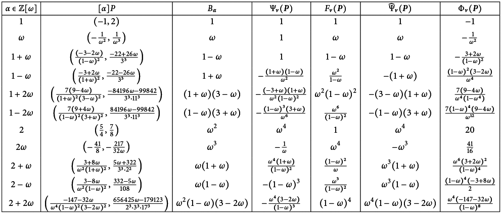


 Open access

