



1. Introduction
The Riemann problem (RP) concerns the evolution of fluid states initially separated by a discontinuity (Riemann Reference Riemann1860). In the context of classical ideal gases, the Euler equations naturally possess hyperbolicity (Godunov Reference Godunov1959; Toro Reference Toro2009), yielding self-similar solutions comprising shock waves, rarefaction waves and contact discontinuities (Dafermos Reference Dafermos2016). Conversely, for real fluids governed by complex thermodynamics, analysing the RP presents more issues. Notably, within rocket engines (Popp et al. Reference Popp, Hulka, Yang and Habiballah2004) and scramjets (Li et al. Reference Li, Wang, Yang, Zhang, Wang, Sun, Wang and Li2023a ), liquid fuels commonly experience a violent expansion-driven phase transition, known as ‘flash evaporation’ (or simply ‘flash’). Currently, accurate physical modelling of flash remains an open question. The RP specifically characterising the flash phenomenon has yet to be formally defined, and its exact solution warrants a comprehensive investigation.
The description of liquid–vapour phase transitions constitutes a longstanding challenge in thermodynamics. Mathematically, there currently exists no single equation of state (EoS) capable of describing the continuous process of fluid phase transitions. Considering the phase diagram of n-dodecane, as shown in figure 1, cubic EoS predict a thermodynamic instability region (Landau & Lifshitz Reference Landau and Lifshitz1980) (bounded by the isothermal spinodal line) and a mechanical instability region (bounded by the isentropic spinodal line) within the saturation envelope. When a state point enters the mechanical instability region, the square of the speed of sound
 $c^2 = (\partial P / \partial \rho )_s$
becomes negative, rendering the Euler equations non-hyperbolic (Menikoff & Plohr Reference Menikoff and Plohr1989). Physically, the liquid–gas phase transition is inherently a non-equilibrium process, accompanied by nucleation and phase-growth dynamics (Lifshitz & Pitaevskii Reference Lifshitz and Pitaevskii1981). These processes introduce a relaxation time or internal length scale into the system. The existence of this physical scale violates the scale invariance of the Euler equations, invalidating classical RP solutions that depend on the self-similar variable (
 $x/t$
).
Phase diagram of n-dodecane.

Figure 1. Long description
A line graph depicting the phase diagram of n-dodecane. The horizontal axis represents the normalized density (rho/rho_c) ranging from 0 to 3.5, and the vertical axis represents the normalized pressure (P/P_c) ranging from 0 to 1.5. The graph includes several curves: a blue saturation curve, a magenta isentropic spinodal curve, and a black isothermal spinodal curve. A red dot marks the critical point, and a shaded gray region indicates where the parameter Gamma is less than 0. The graph also highlights a region labeled Flash evaporation. The isothermal spinodal and the saturation line peak at the same point–the critical point, whereas the density and pressure at the peak of the isentropic spinodal generally differ from those at the critical point.
However, for the specific cases of phase transitions in aerospace propulsion systems, the RP remains amenable to self-similar solutions upon adopting appropriate physical assumptions. As illustrated in figure 2, such flows are ubiquitous in propulsion systems, manifested as spray flows (e.g. transverse jet injection in scramjets (Li et al. Reference Li, Li, Liu, Wang, Sun, Wang, Li, Zhang and Yang2023b
)), frictional pipe flows (e.g. in cooling channels) and expanding pipe flows (e.g. in turbopump nozzles (Cazé et al. Reference Cazé, Petitpas, Daniel, Queguineur and Le Martelot2024)). These flows share a common mechanism: a depressurisation-induced phase transition from liquid to vapour or a two-phase mixture, known as ‘flash evaporation’. Flash flows typically involve intense turbulent mixing or extremely high pressure gradients. This strong thermodynamic driving force causes heterogeneous nucleation to occur extensively within extremely short temporal scales and small spatial scales. Consequently, interphase heat and mass transfer proceeds so rapidly that the non-equilibrium relaxation time (
 $O(10^{-7})$
or even lower; see § 4.1 for detailed analysis) is negligible compared with the macroscopic flow time scale. Therefore, the specific characteristics of the flash phenomenon provide us with the physical basis for constructing its RP: the homogeneous equilibrium model (HEM) (Brennen Reference Brennen2005) and the vapour–liquid equilibrium (VLE) model (Yi et al. Reference Yi, Yang, Habchi and Lugo2019; Yang, Yi & Habchi Reference Yang, Yi and Habchi2020).
Flash evaporation in propulsion systems.

The HEM postulates instantaneous thermodynamic and dynamic equilibrium, where the liquid and vapour phases share identical pressure
 $P$
, temperature
 $T = T_{\textit{sat}}(P)$
and velocity
 $u$
(Brennen Reference Brennen2005). Furthermore, the phase transition is assumed to initiate strictly on the saturation line, neglecting metastable states, and the VLE model is introduced via the equality of fugacity. Combined, the HEM and VLE model construct a stable thermodynamic path, ensuring the equilibrium speed of sound is defined globally and restoring the hyperbolicity of the Euler equations, while simultaneously eliminating the influence of the system’s additional characteristic time scales.
In summary, this paper formalises the flash evaporation Riemann problem (FeRP) as: a RP based on homogeneous equilibrium and vapour–liquid equilibrium assumptions, where the expansion branch crosses the saturation line and induces a liquid–vapour phase transition. This formulation physically captures the flash phenomenon of fluids caused by depressurisation, while mathematically ensuring the self-similarity of the flow and the existence of exact solutions.
The flash process typically involves broad variations in temperature and pressure, thereby invalidating standard ideal gas or liquid assumptions. Consequently, establishing an exact solution for the FeRP requires a preliminary investigation into solutions under thermodynamically stable, single-phase conditions. Colella & Glaz (Reference Colella and Glaz1985) pioneered numerical methods for the RP in real fluid flows. Subsequently, Saurel, Larini & Loraud (Reference Saurel, Larini and Loraud1994) developed an exact Riemann solution for high-temperature real gases and constructed an approximate solution for expansion waves based on the isentropic expansion index. Quartapelle et al. (Reference Quartapelle, Castelletti, Guardone and Quaranta2003) provided a framework for classical real fluids (where
 ${{{\partial }^{2}}e ( v,s )}/{\partial {{v}^{2}}}\;\ne 0$
) by enforcing velocity and pressure continuity across the contact discontinuity. More recently, Wang & Hickey (Reference Wang and Hickey2020) and Wang (Reference Wang2022) constructed an exact RP solution for real fluids that resolves expansion waves based on the concept of generalised Riemann invariants (Kouremenos Reference Kouremenos1986), applying it to transcritical nitrogen flows. In our previous work (Bai et al. Reference Bai, Yang, Xie, Li and Sun2025), we derived a Newton iteration method for the classical RP of two-parameter fluids, grounded in fundamental thermodynamic principles.
A classical solution implies that the wave structure consists solely of expansion rarefaction waves, compression shock waves and contact discontinuities. In Bethe–Zel’dovich–Thompson (BZT) fluids (Lambrakis & Thompson Reference Lambrakis and Thompson1972; Thompson Reference Thompson1972), more complex non-classical wave phenomena may appear, such as expansion shocks and compression fans. The emergence of non-classical waves is determined by the fundamental derivative of gas dynamics
 $\varGamma$
(also known as the Landau derivative, as its significance in gas dynamics was first identified by Landau & Lifshitz (Reference Landau and Lifshitz1959)); the solution is classical when
 $\varGamma \gt 0$
and non-classical otherwise. As shown in figure 1, a region where
 $\varGamma \lt 0$
exists in the supercooled vapour region of n-dodecane (excluding the region inside the spinodal line, which lacks physical meaning). Fortunately, under the VLE model, propulsion fluids of interest such as the kerosene surrogate n-dodecane and the coolant CO
 $_2$
satisfy
 $\varGamma \gt 0$
in both two-phase and single-phase regions; indeed,
 $\varGamma \gt 0$
everywhere except at the saturation line is an implicit prerequisite of the FeRP, distinguishing it from BZT flows. Nevertheless, traversing the saturation line inevitably leads to rarefaction wave splitting and the formation of composite waves containing expansion shocks, which are discussed in § 3. These non-classical waves are physically real; although they violate the Lax entropy condition (Lax Reference Lax1973), they satisfy the more generalised Liu entropy condition (Liu Reference Liu1976). Menikoff & Plohr (Reference Menikoff and Plohr1989) analysed in detail the causes of non-classical waves and the conditions for rarefaction-wave splitting and composite waves in phase-change fluids. Müller & Voss (Reference Müller and Voss2006), Dahmen, Müller & Voss (Reference Dahmen, Müller and Voss2005) and Voss (Reference Voss2005) analysed the construction forms of various non-classical waves in BZT fluids and provided an algorithm based on the topological structure of wave curves, which is capable of resolving diverse non-classical gas-dynamic behaviours. Alternatively, other researchers have investigated specific simplified configurations of the RP involving phase transitions. Saurel et al., based on the stiff EoS and the Noble–Abel stiffened-gas EoS (Saurel, Boivin & Le Métayer Reference Saurel, Boivin and Le Métayer2016), studied the exact solutions (Saurel, Petitpas & Abgrall Reference Saurel, Petitpas and Abgrall2008) and modelling methods (Le Métayer & Saurel Reference Le Métayer and Saurel2016) of phase-change fluids, successfully capturing the phenomenon of rarefaction-wave splitting. Zhao et al. (Reference Zhao, Mentrelli, Ruggeri and Sugiyama2011) investigated the phenomena of shock-induced phase transitions and shock splitting based on the van der Waals EoS. Dreyer, Hantke & Warnecke (Reference Dreyer, Hantke and Warnecke2013) provided the exact solution of the RP for phase-change flows in isothermal processes.
In summary, extensive research has been conducted on the RP for real fluids with phase change, ranging from unified construction methods to those focused on simplified configurations. However, for the specific FeRP, a comprehensive exact solution framework is still lacking. On one hand, the physical behaviour of flash evaporation is well defined, and the non-classical wave structure of the FeRP is deterministic. Consequently, its solution procedure can be more intuitive, eliminating the need for the complex screening and searching processes governed by the Liu entropy condition, which are typically required in algorithms based on wave-curve topologies. On the other hand, flash evaporation often involves substantial state variations. This renders simple models like the stiff EoS insufficient, necessitating more complex EoS such as Peng–Robinson (Peng & Robinson Reference Peng and Robinson1976) or Redlich–Kwong (Redlich & Kwong Reference Redlich and Kwong1949). Therefore, addressing the FeRP, this paper establishes an exact solution framework based on Newton’s method. In § 2, starting from a general EoS
 $P=P(\rho ,T)$
and specific heat function
 $C_v= C_v(\rho ,T)$
, we derive all thermodynamic derivatives for single-phase and equilibrium two-phase fluids, ensuring universality and computational convergence. In § 3, we calculate the fundamental derivative
 $\varGamma$
for common working fluids like n-dodecane and carbon dioxide, analyse their non-classical gas-dynamic behaviours during the flash process and provide exact solution methods for non-classical waves. Finally, we analyse the applicability of the equilibrium assumption and extend the FeRP solution framework with a given thermodynamic non-equilibrium effective speed of sound. Although the thermodynamic closure within the HEM and VLE frameworks uniquely determines the equilibrium speed of sound as the eigenvalue, the complete thermodynamic equilibrium condition may not always accurately describe the actual flow due to nucleation delay and finite-rate heat and mass transfer. Consequently, this extension allows us to systematically investigate the influence of such non-equilibrium effects on wave structures.
2. Exact solution of the flash evaporation Riemann problem
The Euler equations contain three types of discontinuities: shock waves, contact discontinuities and rarefaction waves (the latter being weak discontinuities). This section begins by formulating the thermodynamic relations for single-phase and two-phase regimes, followed by the governing equations for these three discontinuities. Subsequently, we establish a Newton iteration framework to obtain the exact solution of the FeRP.
Prior to deriving the specific governing equations, we first clarify the definitions of ‘single phase’, ‘two phase’ and the aforementioned ‘thermodynamic equilibrium’ adopted in this paper. As shown in figure 3, in thermodynamics, fluid states are classified into thermodynamically stable regions, metastable regions (bounded by the saturation line) and unstable regions (bounded by the spinodal line) (Landau & Lifshitz Reference Landau and Lifshitz1980). As shown in figure 3(a), isentropic lines can cross the saturation line into the metastable region but have no physical meaning inside the spinodal line. Physical phase transitions may occur in the metastable region, where the fluid enters a state of subcooled vapour or superheated liquid after crossing the saturation line, requiring the overcoming of a nucleation barrier to trigger the transition. For instance, previous studies (Saurel et al. Reference Saurel, Petitpas and Abgrall2008; Le Métayer & Saurel Reference Le Métayer and Saurel2016) have modelled phase transitions within the metastable region. Theoretically, one can prescribe a phase-transition initiation boundary (such as the Wilson line (Yellott Reference Yellott1934)) within the metastable region to solve the RP. However, this method presents significant challenges, as it requires not only specifying the location of the phase-transition boundary, but also providing high-order derivatives on the boundary to ensure the proper construction of the wave structures. Furthermore, such an artificial boundary limits the generality of the method.
(a) Thermodynamic boundary and (b) phase model of n-dodecane on the
 $P{-}\rho$
plane.

Accordingly, based on the VLE model, we assume that the flash phase transition initiates strictly at the saturation line, thereby neglecting the delay effects of metastability. As shown in figure 3(b), throughout this paper, the ‘two-phase region’ (or mixture region) refers to the area enclosed by the saturation line, while the ‘single-phase region’ denotes the area outside the saturation line, corresponding to the ‘thermodynamically stable region’. Through the condition of equal fugacity, the VLE model constructs a continuous equilibrium trajectory across the two-phase region, permitting isentropes to cross the saturation lines continuously.
2.1. Governing equations and basic thermodynamic parameters
The governing equations for the RP are the one-dimensional Euler equations:
 \begin{equation} \frac {\partial \boldsymbol{U}}{\partial t}+\frac {\partial \boldsymbol{F}(\boldsymbol{U})}{\partial x}=0, \end{equation}
where
 $\boldsymbol{U}$
is the vector of conserved variables and
 $\boldsymbol{F}$
is the flux vector. Their specific expressions are
 \begin{equation} \boldsymbol{U}=\left ( \begin{matrix} \rho \\ \rho u \\ \rho \left(e+\dfrac {1}{2}{{u}^{2}}\right) \\ \end{matrix} \right )\!,\quad \boldsymbol{F}=\left (\begin{matrix} \rho u \\ \rho {{u}^{2}}+P \\ \rho u \left(e+\dfrac {1}{2}{{u}^{2}}\right)+Pu \\ \end{matrix} \right )\!. \end{equation}
The thermodynamic relations are detailed below for the single-phase fluid and the two-phase mixture.
-
(i) For the single-phase fluid: The EoS adopts
 $\rho$
and
$T$
as independent variables, defining
$P$
as:(2.3)Here,
\begin{equation} P=P\left ( \rho ,T \right )\!. \end{equation}
$P$
is a single-valued function of
$\rho$
and
$T$
, and
$T$
is also uniquely determined by
$P$
and
$\rho$
(note that
$\rho$
is not necessarily a single-valued function of
$P$
and
$T$
).
The internal energy is expressed as
(2.4)where
\begin{equation} e(\rho ,T)=\int _{{{T}_{0}}}^{T}{{{C}_{v}}\,\mathrm{d}T}-\int _{{{\rho }_{0}}}^{\rho }{\frac {1}{{{\rho }^{2}}}\left ( T\left (\frac {\partial P}{\partial T}\right )_{\rho }-P \right )}\mathrm{d}\rho +e_0, \end{equation}
$C_v$
is the specific heat at constant volume. Parameter
$C_v$
is also a function of
$\rho$
and
$T$
, which is often termed the caloric equation of state:(2.5)
\begin{equation} {C_v}={C_v}(\rho ,T). \end{equation}
The entropy expression for the single-phase fluid is
(2.6)
\begin{equation} s(\rho ,T)=\int _{{{T}_{0}}}^{T}{\frac {{{C}_{v}}}{T}\,\mathrm{d}T}-\int _{{{\rho }_{0}}}^{\rho }{\frac {1}{{{\rho }^{2}}}{\left (\frac {\partial P}{\partial T}\right )_{\rho }}\mathrm{d}\rho }+s_0. \end{equation}
The speed of sound for the single-phase fluid is
(2.7)
\begin{equation} {c^2}= \left (\frac {\partial P}{\partial \rho }\right )_{s}=\left (\frac {\partial P}{\partial \rho }\right )_{T}+\frac {T}{{{C}_{v}}{{\rho }^{2}}}\left (\frac {\partial P}{\partial T}\right )_{\rho }^{2}. \end{equation}
-
(ii) For the two-phase mixture:
$P$
takes
$T$
as the unique independent variable. The
$P{-}T$
curve is referred to as the saturation line:(2.8)Each point
\begin{equation} P=P_{\textit{sat}}\left (T \right )\!. \end{equation}
$(P,T)$
on the saturation line corresponds to two density values: the saturated vapour density
$\rho _v$
and the saturated liquid density
$\rho _l$
. The two-phase equilibrium mixture density
$\rho$
and the saturation densities satisfy the relation (consistent with the lever rule)(2.9)where
\begin{equation} \rho =\alpha \rho _v +(1-\alpha )\rho _l, \end{equation}
$\alpha$
is the vapour volume fraction. Equation (2.9) is equivalent to(2.10)
\begin{equation} \alpha (\rho ,T)=\frac {\rho -\rho _l(T)}{\rho _v(T) - \rho _l(T)}. \end{equation}


The internal energy expression for the two-phase mixture is
 \begin{equation} e(\rho ,T)=\frac {\alpha \rho _v(T) e_v(T) +(1-\alpha )\rho _l(T) e_l(T)}{\rho }, \end{equation}
where
 $e_v$
and
 $e_l$
are the internal energies on the vapour and liquid saturation lines at
 $(P,T)$
, respectively; clearly, these depend solely on
 $T$
(or
 $P$
).
The entropy expression for the two-phase mixture is analogous to internal energy. Defining
 $s_v$
and
 $s_l$
as the entropy at point
 $(P,T)$
on the saturation lines:
 \begin{equation} s(\rho ,T)=\frac {\alpha \rho _v(T) s_v(T) +(1-\alpha )\rho _l(T) s_l(T)}{\rho }. \end{equation}
The complete thermodynamic equilibrium speed of sound for the two-phase mixture is calculated from the ratio of the derivatives of mixture entropy with respect to density and pressure. This simplifies to
 \begin{equation} \frac {1}{\rho c_{eq}^2}=\frac {\alpha }{{\rho _v}c_v^2}+\frac {1-\alpha }{{\rho _l}c_l^2}+T\left ( \frac {\alpha {\rho _v}}{{C_{P,v}}}{{\left ( \frac {\mathrm{d}s_v}{\mathrm{d}P} \right )}^{2}}+\frac {(1-\alpha ){\rho _l}}{C_{P,l}}{{\left ( \frac {\mathrm{d}s_l}{\mathrm{d}P} \right )}^{2}} \right )\!, \end{equation}
where
 $c_v$
,
 $c_l$
and
 $C_{P,v}$
,
 $C_{P,l}$
are the speed of sound and specific heat at constant pressure at
 $(P,T)$
on the saturation line, respectively. Clearly, they are also single-valued functions of
 $P$
or
 $T$
. In addition,
 $C_v$
and
 $C_P$
satisfy the thermodynamic relation (Sedov Reference Sedov1973):
 \begin{equation} {C_P}-{C_v}=\frac {T}{{\rho ^2}}\frac {\left ( {\partial P}/{\partial T} \right )_\rho ^2}{{\partial P}/{\partial \rho }}. \end{equation}
It should be noted that the expressions for the speed of sound in (2.7) and (2.13) are strictly equivalent. The derivation of their equivalence can be found in Saurel et al. (Reference Saurel, Petitpas and Abgrall2008). Furthermore, (2.13) has other equivalent forms, such as the one presented in Michaelides & Zissis (Reference Michaelides and Zissis1983).
Additionally, under the above definition, the latent heat of vaporisation is intrinsically encapsulated within the mixture EoS, ensuring that the energy cost of phase change is dynamically compensated by the fluid’s sensible heat release during the isentropic depressurisation.
2.2. Types of discontinuities in the flash evaporation Riemann problem
The governing equations for these three types of discontinuities are identical to those for non-phase-changing real fluids (Bai et al. Reference Bai, Yang, Xie, Li and Sun2025). Shock waves satisfy the Rankine–Hugoniot conditions, contact discontinuities satisfy velocity and pressure equilibrium conditions and rarefaction waves follow isentropic relations, resolved via the method of characteristics. Denoting the pre-wave state by subscript ‘1’ and the post-wave state by subscript ‘2’, the governing equations are as follows.
2.2.1. Shock wave
The upstream and downstream states of a shock correspond to the intersection of the Hugoniot curve with the Rayleigh line. The Hugoniot relation is expressed as
 \begin{equation} {e_1}-{e_2}+\frac {P_1}{\rho _1}-\frac {P_2}{\rho _2}+\frac {(P_2-P_1)(\rho _1+\rho _2)}{2\rho _1 \rho _2}=0. \end{equation}
The Rayleigh line is defined by
 \begin{equation} \frac {P_2 - P_1}{1/\rho _2 - 1/\rho _1} = - (\rho _1 u_1)^2 = - (\rho _2 u_2)^2 = - j^2, \end{equation}
where
 $j$
represents the mass flux.
2.2.2. Contact discontinuity
The states on either side of a contact discontinuity satisfy the relation
 \begin{equation} {u_1}={u_2}; \quad {P_1}={P_2}. \end{equation}
2.2.3. Rarefaction wave
Rarefaction waves are classified as weak discontinuities characterised by continuous state variables but discontinuous derivatives. They are solved analytically via the method of characteristics. Along a characteristic line within the wave
 \begin{equation} \frac {\mathrm{d}x}{\mathrm{d}t}=u\pm c, \end{equation}
the Riemann invariants are
 \begin{equation} {{J}^{\pm }}=u\pm \int _{{{C}^{\pm }}}{\frac {1}{\rho c}\mathrm{d}P}=\text{const}. \end{equation}
For a left-propagating rarefaction wave, the Riemann invariant
 $J^+$
(associated with the right-propagating characteristic
 $C^+$
) remains constant across the wave. Consequently, the signs in (2.18) and (2.19) both take ‘
 $+$
’. Conversely, for a right-propagating rarefaction wave, the Riemann invariant
 $J^-$
(associated with the left-propagating characteristic
 $C^-$
) remains constant. Thus, the signs in (2.18) and (2.19) both take ‘
 $-$
’.
2.3. Types of solution curves for the flash evaporation Riemann problem
During the flash process, the liquid undergoes a phase transition due to expansion. Depending on fluid properties and equilibrium pressure, the liquid may expand into the two-phase region or traverse it entirely into the vapour phase. Meanwhile, the low-pressure gas on the other side is subjected to compression. Without loss of generality, we specify the left state of the FeRP as a high-pressure liquid and the right state as a low-pressure gas. Other cases, such as double rarefaction waves, follow similar principles and are omitted for brevity. Considering practical situations (e.g. fuel sprays in engines), we assume the low-pressure gas on the right side is sufficiently far from the saturation line and remains in the vapour phase state during compression.
We analyse the solution curves of the RP on the
 $P{-}v$
diagram (
 $v=1/\rho$
denotes specific volume). Depending on the initial state and thermodynamic properties of the fluid, the FeRP yields three distinct solution types: the R-S (rarefaction wave–shock wave) solution, the RS-S (rarefaction–upstream sonic expansion shock composite wave–shock wave) solution and the RSR-S (rarefaction–double sonic expansion shock–rarefaction composite wave–shock wave) solution, as illustrated in figure 4. In figure 4, the compression branch follows a Hugoniot curve in the vapour phase, whereas the expansion branch comprises either a pure isentrope or a composite path involving Hugoniot segments. We specify
 $P_{\textit{S},1}$
and
 $P_{\textit{S},2}$
as the intersections of the isentrope with the liquid and vapour saturation lines, respectively. Furthermore,
 $P_{\textit{CJ},1}$
and
 $P_{\textit{CJ},2}$
represent the pre-shock and post-shock pressures of the unique double sonic shock along a given isentrope. The resulting wave structure is determined by the intermediate pressure
 $P^*$
relative to these characteristic pressures:
-
(i)
$ P_{\textit{S},1} \gt P^* \gt P_{\textit{S},2}$
: The expansion branch is a single rarefaction wave, denoted as an R wave. Although the wave splits at
$P_{\textit{S},1}$
due to the discontinuity in the speed of sound, the integration of the Riemann invariants remains unaffected. -
(ii)
$ P_{\textit{S},2} \gt P^* \gt P_{\textit{CJ},2}$
: The expansion branch forms a composite wave comprising a rarefaction wave and an upstream sonic expansion shock (where the pre-shock state satisfies the Chapman–Jouguet (CJ) condition), denoted as an RS wave. The transition occurs at a CJ state point
$a$
, where
$P_a \in (P_{\textit{CJ},1}, P_{\textit{S},2})$
. The expansion shock connects
$P_a$
to the post-shock pressure
$P^*$
. -
(iii)
$ P_{\textit{CJ},2} \gt P^*$
: The expansion branch is a composite structure consisting of a head rarefaction wave, a double sonic expansion shock (which achieves CJ states both upstream and downstream) and a tail rarefaction wave, denoted as an RSR wave. The double sonic shock bridges the two CJ states
$P_{\textit{CJ},1}$
and
$P_{\textit{CJ},2}$
, connecting the head rarefaction to the tail rarefaction, which subsequently extends to the intermediate pressure
$P^*$
.


Three types of solution curves for the flash RP, using the n-dodecane phase diagram as an example.

Figure 4. Long description
A line graph showing the relationship between the normalized pressure (P/Pc) and the normalized specific volume (v/vc). The graph includes three main curves: the saturation curve in black, the expansion branch in blue, and the compression branch in magenta. Key points on the graph are marked with red dots and labeled as PS,1, PCJ,1, PS,2, and PCJ,2. The graph also shows contact discontinuities with black dashed lines labeled as R-S, RS-S, and RSR-S. The saturation curve peaks around a normalized specific volume of 1 and then declines. The expansion branch starts high and decreases steadily, while the compression branch starts lower and also decreases but at a different rate. The contact discontinuities connect points on the expansion and compression branches, indicating transitions between different states.
For a given left state, the characteristic pressures
 $P_{\textit{S},1},\ P_{\textit{S},2},\ P_{\textit{CJ},1}$
and
 $P_{\textit{CJ},2}$
are solely determined by the initial conditions, independent of the intermediate pressure
 $P^*$
. In contrast, although the transition pressure
 $P_a$
varies with
 $P^*$
, its determination relies on the same mathematical formulation as that derived for solving
 $P_{\textit{CJ}}$
. Given that the iterative solution for these values involves complex derivations, we assume in this section that these parameters are known, in order to maintain focus on the core algorithm of the exact Riemann solution. It should be noted that the existence of
 $P_{\textit{CJ},1}$
,
 $P_{\textit{CJ},2}$
and
 $P_a$
depends on the fluid properties. For certain fluids, the FeRP exclusively admits solutions of the R-S form. The specific calculations of these values, along with further analysis of the expansion branch, are detailed in § 3.
2.4. Method for solving intermediate pressure in flash evaporation Riemann problem
The primary objective of solving the RP is to determine the intermediate pressure
 $P^*$
and velocity
 $u^*$
such that pressure and velocity remain continuous across the contact discontinuity:
 \begin{equation} u_L^* = u_R^* = u^* \quad \text{and} \quad P_L^* = P_R^* = P^*. \end{equation}
We employ Newton’s method with the intermediate pressure
 $P^*$
as the iteration variable. For a given estimate
 $P^*$
, the residual function
 $U(P^*)$
is defined as the velocity difference at the contact discontinuity:
 \begin{equation} U(P^*) = (u_L + \psi _L(P^*)) - (u_R - \varphi _R(P^*)) = 0, \end{equation}
where
 $\psi _L$
represents the velocity variation across the expansion branch (R, RS or RSR wave), referred to as the expansion
 $P{-}u$
function. Similarly,
 $\varphi _R$
represents the velocity variation across the compression branch (S wave), referred to as the compression
 $P{-}u$
function. The Newton iteration formula is
 \begin{equation} P_{k+1}^* = P_k^* - \frac {U\left(P_k^*\right)}{U'\left(P_k^*\right)}. \end{equation}
Consequently, the key to solving for the intermediate pressure lies in deriving
 $U(P^*)$
and its derivative
 $U'(P^*)$
.
2.4.1. Compression branch
$\varphi _R$

As previously stated, the compression branch consists of a single shock wave. The function
 $\varphi _R(P^*)$
represents the shock
 $P{-}u$
relation:
 \begin{equation} \varphi _{R}(P^*)={{j}_{R}}\left ( \frac {1}{\rho _{R}^{*}}-\frac {1}{{\rho _R}} \right )\!, \end{equation}
where
 $j$
is the mass flux through the shock, determined by (2.16), and
 $P^*$
and
 $\rho _R^*$
satisfy the Hugoniot relation (2.15).
The derivative of
 $\varphi _R(P)$
with respect to
 $P$
is
 \begin{equation} \frac {\mathrm{d} {{\varphi }_{R}}}{\mathrm{d}{{P}^{*}}}=-\frac {1}{2{{j}_{R}}}-\frac {{{j}_{R}}}{2(\rho _R^*)^2}{\left ( \frac {\mathrm{d}\rho }{\mathrm{d}P} \right )}_{H,R}, \end{equation}
where
 ${({\mathrm{d}\rho }/{\mathrm{d}P})}_{H,R}$
represents the derivative along the Hugoniot curve at the state
 $(P^*, \rho _R^*)$
:
 \begin{equation} {\left ( \frac {\mathrm{d}\rho }{\mathrm{d}P} \right )}_{H,R}=-\frac {(\partial {F_H}/\partial {P^*})_{\rho }}{(\partial {F_H}/\partial {\rho })_{P^*}} = -\frac {- \left (\dfrac {\partial e}{\partial P}\right )_{\rho }+\dfrac {\rho - \rho _R}{2 \rho \rho _R}}{- \left (\dfrac {\partial e}{\partial \rho }\right )_{P}+\dfrac {P^*+P_R}{2 \rho ^2}}. \end{equation}
To calculate
 $\varphi _R(P)$
and its derivative, a nested Newton iteration is required to determine the post-shock density
 $\rho _R^*$
corresponding to
 $P^*$
that satisfies the Hugoniot relation.
Let the residual function be the Hugoniot condition:
 \begin{equation} F_H = e(\rho ,P^*)-e(\rho _R,P_R)+\frac {P_R}{\rho _R}-\frac {P^*}{\rho }+\frac {(P^*-P_R)(\rho _R+\rho )}{2\rho _R \rho }=0. \end{equation}
Its derivative is
 \begin{equation} \left (\frac {\partial F_H}{\partial \rho }\right )_{P^*} = - \left (\frac {\partial e}{\partial \rho }\right )_{P}+\frac {P^*+P_R}{2 \rho ^2}. \end{equation}
Note that the internal energy depends on pressure and density via
 $e(\rho ,P)=e(\rho ,T(\rho ,P))$
. Computing
 $e$
via (2.4) or (2.11) requires an iterative inversion of the EoS (2.3) to obtain
 $T$
in the single-phase region; in the two-phase region, however, the temperature is explicitly determined by
 $T=T_{\textit{sat}}(P)$
. The algorithm for this iterative procedure can be found in Bai et al. (Reference Bai, Yang, Xie, Li and Sun2025). The analytical expressions for
 $({\partial e}/{\partial \rho })_{P}$
and
 $({\partial e}/{\partial P})_{\rho }$
are provided in Appendix C.1.
2.4.2. Expansion branch
$\psi _L$
– R wave

When
 $ P_{\textit{S},1} \gt P^* \gt P_{\textit{S},2}$
, the expansion branch is a single rarefaction wave. Although this rarefaction wave exhibits splitting behaviour, the flow remains isentropic, and the definition of the Riemann invariant remains valid. This case represents the simplest configuration, where the expansion
 $P{-}u$
function is directly derived from the Riemann invariant:
 \begin{equation} \psi _L(P^*) = \int _{P^*}^{P_L} \frac {1}{\rho c}\,\mathrm{d}P. \end{equation}
This integral is evaluated using numerical integration algorithms (Bai et al. Reference Bai, Yang, Xie, Li and Sun2025). Along the integration path,
 $\rho$
and
 $P$
satisfy the isentropic relation, and
 $c = c_{eq}(\rho ,P)$
.
The derivative of
 $\psi _L(P^*)$
is
 \begin{equation} \frac {\mathrm{d}\psi _L}{\mathrm{d}P^*} = - \frac {1}{\rho ^*_L c^*_L}. \end{equation}
To calculate
 $\psi (P)$
and its derivative, a nested Newton iteration is needed to determine
 $\rho , c$
corresponding to
 $P^*$
subject to the isentropic relation.
Let the residual function be the isentropic condition:
 \begin{equation} F_s = s(\rho _L,P_L) - s(\rho ,P). \end{equation}
Note that entropy depends on density and pressure via
 $s(\rho ,P)=s(\rho ,T(\rho ,P))$
. The derivative of this residual function is
 \begin{equation} \left (\frac {\partial F_s}{\partial \rho }\right )_{P} = -\left (\frac {\partial s}{\partial \rho }\right )_{P}, \end{equation}
where the analytical expression for
 $({\partial s}/{\partial \rho })_{P}$
is provided in Appendix C.1.
2.4.3. Expansion branch
$\psi _L$
– RS wave

When
 $ P_{\textit{S},2} \gt P^* \gt P_{\textit{CJ},2}$
, the expansion branch is a composite wave consisting of a rarefaction wave and an upstream sonic expansion shock. We denote the transition point – where the rarefaction terminates and the shock initiates – as state
 $a$
. At point
 $a$
, the shock wave is co-moving with the tail of the rarefaction wave; specifically, the propagation speed of the shock equals the characteristic speed of the rarefaction-wave tail. This is also referred to as the CJ condition, where the mass flux satisfies
 $j_a = \rho _a c_a$
. The
 $P{-}u$
function of the RS wave is given by
 \begin{equation} \psi _L(P^*) = - \int _{P_L}^{P_a} \frac {1}{\rho c}\,\mathrm{d}P + \frac {P_a-P^*}{j_a}. \end{equation}
The derivative of
 $\psi _L(P^*)$
is
 \begin{equation} \frac {\mathrm{d}\psi _L}{\mathrm{d}P^*} = - \frac {1}{j_a}\left (1+ \frac {P_a-P^*}{j_a}\frac {\mathrm{d}j_a}{\mathrm{d}P_a}\frac {\mathrm{d}P_a}{\mathrm{d}P^*} \right )\!, \end{equation}
where the transition pressure
 $P_a$
resides within the interval
 $(P_{\textit{CJ},1}, P_{\textit{S},2})$
. Note that in deriving (2.33), the derivative terms associated with the variation of the transition point
 $P_a$
in the rarefaction and shock portions cancel out due to the CJ condition. The methodology for determining
 $P_a$
, as well as the analytical expressions for
 ${\mathrm{d}j_a}/{\mathrm{d}P_a}$
and
 ${\mathrm{d}P_a}/{\mathrm{d}P^*}$
, are detailed in the subsequent section after introducing the double sonic shock. The path from
 $P_L$
to
 $P_a$
represents a single rarefaction wave, the calculation of which is analogous to that described in the preceding subsection.
2.4.4. Expansion branch
$\psi _L$
– RSR wave

When
 $ P_{\textit{CJ},2} \gt P^*$
, the expansion branch is a composite wave consisting of a head rarefaction, a double sonic expansion shock and a tail rarefaction wave. We denote the upstream CJ state point CJ,1 as the transition point where the head rarefaction terminates and the shock initiates, while the downstream CJ state point CJ,2 marks the transition point from the shock to the tail rarefaction. In this configuration, the shock flux satisfies the dual CJ condition:
 $j_{\textit{CJ}} = \rho _{\textit{CJ},1} c_{\textit{CJ},1} = \rho _{\textit{CJ},2} c_{\textit{CJ},2}$
. The
 $P{-}u$
function of the RSR wave is given by
 \begin{equation} \psi _L(P^*) = - \int _{P_L}^{P_{\textit{CJ},1}} \frac {1}{\rho c}\,\mathrm{d}P + \frac {P_{\textit{CJ},1}-P_{\textit{CJ},2}}{j_{\textit{CJ}}}- \int _{P_{\textit{CJ},2}}^{P^*} \frac {1}{\rho c}\,\mathrm{d}P. \end{equation}
The derivative of
 $\psi _L(P^*)$
is
 \begin{equation} \frac {\mathrm{d}\psi _L}{\mathrm{d}P^*} = - \frac {1}{\rho ^*_L c^*}. \end{equation}
Note that the Riemann invariant for the tail rarefaction wave is integrated along the isentrope originating from
 $P_{\textit{CJ},2}$
to
 $P^*$
. This isentrope is distinct from the integration isentrope of the head rarefaction wave (which starts from the initial left state), as the entropy increases across the expansion shock.
2.5. State solution inside split rarefaction waves
The ultimate objective of solving the RP is to obtain the flow state at any characteristic coordinate
 $\xi = x/t$
. After determining the intermediate pressure, it is necessary to consider the relative position of the wave structure and the coordinate
 $\xi$
to calculate the flux. The calculation of fluxes in the undisturbed and intermediate regions is straightforward and analogous to the ideal gas case, so it is omitted here. However, determining the flux within a rarefaction wave is more complex, specifically due to the wave splitting arising from the discontinuous drop in the speed of sound across the saturation boundary. This requires a solution strategy distinct from that for single-phase fluids (Bai et al. Reference Bai, Yang, Xie, Li and Sun2025). Based on the preceding discussion, we provide a Newton iteration method specifically tailored for this scenario. Considering a left-propagating R wave (also applicable to rarefaction segments within RS and RSR structures), the rarefaction fan spans the domain defined by
 \begin{equation} {\lambda _{\textit{head}}}\lt \frac {x}{t}\lt {\lambda _{\textit{tail}}}, \end{equation}
where
 $\lambda _{\textit{head}} = u_L-c_L$
denotes the velocity of the rarefaction wave head and
 $\lambda _{\textit{tail}}$
denotes the wave tail velocity, defined as
 \begin{equation} \lambda _{\textit{tail}} = \begin{cases} u^* - c^* & \text{R wave}, \\ u_a - c_a & \text{RS wave}, \\ u_{\textit{CJ},1} - c_{\textit{CJ},1} & \text{RSR wave}. \end{cases} \end{equation}
However, traversing the liquid saturation boundary (point
 $S,1$
in figure 4) induces a discontinuous drop in the speed of sound, leading to a discontinuity in the characteristic wave speed. The saturation point
 $S,1$
is characterised by two distinct sound speeds: the liquid speed
 $c=c_{l,\text{S}}$
and the equilibrium speed
 $c=c_{eq,\text{S}}$
, defined as
 \begin{equation} c_{eq,\text{S}} = \left (\frac {1}{c^2_{l,\text{S}}} + \frac {\rho ^2_{l,\text{S}}}{C_{P,l\text{S}}}{{\left ( \frac {\mathrm{d}s_l}{\mathrm{d}P} \right )}^{2} }\right )^{-1/2}. \end{equation}
The characteristic wave speeds satisfy
 $\lambda _{l,\text{S}} = u_S - c_{l,\text{S}} \lt u_S - c_{eq,\text{S}} = \lambda _{eq,\text{S}}$
. Since the rarefaction wave is left-propagating, this sudden increase in characteristic wave speed causes the wave to split at point
 $S,1$
. The wave segment in the characteristic speed interval
 $(\lambda _{\textit{head}}, \lambda _{l,\text{S}})$
travels faster in the negative
 $x$
direction than the segment in the interval
 $(\lambda _{eq,\text{S}}, \lambda _{\textit{tail}})$
, leading to the splitting of the rarefaction wave in the
 $x{-}t$
diagram. It is crucial to distinguish rarefaction wave splitting from a discontinuity. The split rarefaction wave remains continuous on the
 $P{-}v$
diagram (following the isentrope), but a constant state region manifests on the
 $x{-}t$
diagram. In contrast, a true discontinuity involves a jump in thermodynamic states on the
 $P{-}v$
diagram governed by the Rankine–Hugoniot relations. For instance, a double sonic shock in RSR wave may be considered as a ‘discontinuity’ embedded within a rarefaction wave (though this analogy is imperfect as the two R components of an RSR wave do not share the same isentrope).
In summary, the rarefaction wave in the classical sense (characterised by continuous wave-speed variation) exists only when the coordinate
 $\xi$
lies within the characteristic speed intervals
 $(\lambda _{\textit{head}}, \lambda _{l,\text{S}})$
and
 $(\lambda _{eq,\text{S}}, \lambda _{\textit{tail}})$
. For coordinates within these two intervals, we use Newton’s method to resolve the internal wave structure. Denoting the known pre-wave state by the subscript ‘1’ and the unknown state to be resolved by subscript ‘0’, the residual function is written as
 \begin{equation} \begin{aligned} & u_1+\int _{P_1}^{P_1}{\frac {1}{\rho c}\mathrm{d}P}= u_0+\int _{P_0}^{P_1}{\frac {1}{\rho c}\mathrm{d}P} = c_0 +\frac {x}{t}-\int _{P_0}^{P_1}{\frac {1}{\rho c}\mathrm{d}P} \\ &\quad \Rightarrow F_R = c\left ( \rho _0,P_0 \right )+\frac {x}{t}-u_1+\int _{P_0}^{P_1}{\frac {1}{\rho c}\mathrm{d}P} =0. \end{aligned} \end{equation}
Differentiating
 $F_R$
with respect to
 $\rho$
and substituting the definition of the isentropic speed of sound
 ${c^2}= ({\partial P}/{\partial \rho })_{s}$
, we obtain
 \begin{equation} \left (\frac {\partial F_R}{\partial \rho _0}\right )_{P_0}= \left . {\left (\frac {\partial c}{\partial \rho }\right )_{P}} \right |_{P=P_0} + \left . {\left (\frac {\partial c}{\partial P}\right )_{\rho }} \right |_{\rho =\rho _0} c^2_0 + \frac {c_0}{\rho _0}, \end{equation}
where the analytical expressions for
 $({\partial c}/{\partial \rho })_{P}$
and
 $({\partial c}/{\partial P})_{\rho }$
are given in Appendix F. These expressions are also instrumental in the evaluation of the fundamental derivative
 $\varGamma$
discussed later.
When the coordinate
 $\xi$
lies within the interval
 $(\lambda _{l,\text{S}}, \lambda _{eq,\text{S}})$
, the state remains constant in the
 $x{-}t$
plane (corresponding to point
 $S,1$
in the
 $P{-}v$
plane):
 \begin{equation} u=u_S; \quad P=P_S; \quad \rho =\rho _s. \end{equation}
These values can be determined from the initial state via isentropic relations.
It is worth noting that for the Newton iteration algorithm designed for flash rarefaction waves, we select
 $\rho$
as the iteration variable rather than
 $P$
, contrasting with the approach in Bai et al. (Reference Bai, Yang, Xie, Li and Sun2025). This choice is motivated by the fact that when the isentrope crosses the liquid saturation boundary into the two-phase region (particularly at low pressures), the speed of sound drops significantly, causing the isentrope to become very flat in the
 $P{-}\rho$
plane. If pressure were used as the iteration variable, small pressure perturbations would result in large density variations, making convergence difficult or impossible. Numerical experiments confirm that selecting
 $\rho$
as the independent variable confers robust convergence characteristics.
3. Non-classical waves in the flash evaporation Riemann problem and their solution methods
As previously discussed, the FeRP admits three types of wave structures: rarefaction waves, RS composite waves, and RSR composite waves. The physical mechanisms underpinning non-classical waves in BZT and phase-changing fluids have been analysed in detail by Menikoff & Plohr (Reference Menikoff and Plohr1989) and Dahmen et al. (Reference Dahmen, Müller and Voss2005). Building upon their findings, this section investigates the properties of these waves, specifically from the perspective of solution algorithm design.
3.1. Fundamental derivative of classical equilibrium phase-change fluids
The sign and smoothness of the fundamental derivative determine whether the fluid dynamics exhibit ‘classical’ behaviour. It is defined as
 \begin{equation} \varGamma = -\frac {v}{2}\frac {\partial ^2 P(v,s)/\partial v^2}{\partial P(v,s)/\partial v}. \end{equation}
Through algebraic manipulation,
 $\varGamma$
can be reformulated in terms of the thermodynamic derivatives obtained previously:
 \begin{equation} \varGamma = 1+\frac {\rho }{c} \left (c^2\left (\frac {\partial c}{\partial P}\right )_{\rho } +\left (\frac {\partial c}{\partial \rho }\right )_{P} \right )\!, \end{equation}
where the analytical expansions of
 $({\partial c}/{\partial \rho })_{P}$
and
 $({\partial c}/{\partial P})_{\rho }$
are detailed in Appendices C and F. Clearly, the term in the brackets
 \begin{equation} c^2\left (\frac {\partial c}{\partial P}\right )_{\rho } +\left (\frac {\partial c}{\partial \rho }\right )_{P} = \left (\frac {\partial c}{\partial \rho }\right )_{s} \end{equation}
represents the derivative of the speed of sound with respect to density along the isentrope, which also reflects the intrinsic link between rarefaction-wave properties and the value of
 $\varGamma$
. Fundamentally, the value of
 $\varGamma$
characterises the convexity of the isentrope. When
 $\varGamma \gt 0$
and strict smoothness holds globally, the isentrope is smooth and globally convex, and the wave dynamic behaviour of the fluid is classical; otherwise, non-classical waves appear.
In this paper, we consistently employ the Peng–Robinson (PR) EoS to evaluate the fundamental derivative
 $\varGamma$
, resolve phase equilibrium and compute the Riemann solution. The PR EoS is widely adopted in the chemical engineering field and demonstrates high predictive accuracy for propulsion working fluids such as
 $\text{CO}_2$
,
 $\text{CH}_4$
, n-dodecane and other hydrocarbon gases over a wide pressure range. For the calculation of internal energy and entropy, we use exact integration based on the PR EoS (see Guardone & Argrow (Reference Guardone and Argrow2005) for details), with the corresponding coefficients calibrated against NIST data (NIST 2023). The expressions for the PR EoS, its thermodynamic derivatives and the values of related coefficients are provided in Appendices A and G.
Figure 5 illustrates the fundamental derivative
 $\varGamma$
for n-dodecane calculated via the PR EoS. Specifically, figure 5(a) depicts the distribution of
 $\varGamma$
computed directly without incorporating the VLE model. The derivative
 $\varGamma$
diverges to infinity at the isentropic spinodal line (
 $c^2=0$
), which is evident from the denominator in (3.2). For the majority of fluids (such as
 $\text{CO}_2$
,
 $\text{N}_2$
and
 $\text{O}_2$
), the domain where
 $\varGamma \lt 0$
is totally enclosed by the isothermal spinodal line; consequently, these regions are excluded from consideration as they lack physical meaning. What is of real concern is the scenario where the
 $\varGamma \lt 0$
region extends outside the spinodal line, as observed in the supercooled vapour of n-dodecane (see figure 1). However, upon incorporating the VLE model, we observe that
 $\varGamma$
for n-dodecane remains positive and smooth throughout the entire domain, except at the saturation line, as demonstrated in figure 5(b). Common propellants of interest, such as
 $\text{CO}_2$
,
 $\text{N}_2$
,
 $\text{O}_2$
and
 $\text{CH}_4$
, share this characteristic. Consequently, the analysis of the wave structure in the FeRP reduces to considering non-classical waves solely at the phase boundaries.
Fundamental derivative
 $\varGamma$
of n-dodecane (a) without and (b) with the VLE model.

There is a theoretical detail in figure 5 that cannot be captured by numerical calculations. Revisiting the definition of
 $\varGamma$
in (3.2), the discontinuous jump in the speed of sound at the phase boundary induces a divergence in
 $({\partial c}/{\partial \rho })_{P}$
and
 $({\partial c}/{\partial P})_{\rho }$
, which manifests in
 $\varGamma$
as a local Dirac ‘
 $\delta$
-function’ singularity on the saturation line. The impact of this singularity on the wave structure varies according to the fluid properties:
-
(i) When the isentrope crosses the liquid saturation line, the characteristic speed always exhibits a positive jump
$\lambda _{l} \lt \lambda _{eq}$
. Consequently,
$\varGamma$
exhibits a positive
$\delta$
-function singularity. The condition
$\varGamma \gt 0$
still holds globally, and a split rarefaction wave exists without non-classical waves. -
(ii) For the vapour saturation line, the direction in which the isentrope crosses varies for different fluids. For fluids with high specific heat capacity (such as n-dodecane), the isentrope crosses from the two-phase region into the gas-phase region, which corresponds to a retrograde crossing direction, as shown in figure 6(a). In this configuration, the characteristic speed exhibits a negative jump
$\lambda _{eq} \Rightarrow \lambda _{v}$
, with
$\lambda _{eq} \gt \lambda _{v}$
. Consequently,
$\varGamma$
exhibits a negative
$\delta$
-function singularity, locally violating the condition
$\varGamma \gt 0$
and giving rise to RS or RSR composite waves. -
(iii) For general low-heat-capacity, low-molecular-weight fluids (such as
$\text{CO}_2$
,
$\text{CH}_4$
,
$\text{O}_2$
), expansion drives the isentrope deeper into the two-phase region but does not cross the vapour saturation line retrogradely. Therefore, the isentrope only crosses from the vapour-phase region into the two-phase region, as shown in figure 6(b). In this configuration, the characteristic speed exhibits a positive jump
$\lambda _{v} \Rightarrow \lambda _{eq}$
. Consequently,
$\varGamma$
exhibits a positive
$\delta$
-function singularity, and only a split rarefaction wave exists.


In summary, the dynamic condition for the emergence of non-classical waves is a retrograde jump in characteristic speed – thermodynamically equivalent to the manifestation of a negative
 $\delta$
-function singularity in
 $\varGamma$
– which consequently gives rise to RS and RSR composite waves. This phenomenon occurs during the flash evaporation of high-heat-capacity fluids like n-dodecane. Conversely, for fluids like
 $\text{CO}_2$
,
 $\text{CH}_4$
and
 $\text{O}_2$
, non-classical waves are absent, and only rarefaction-wave splitting occurs.
In addition, when gaseous n-dodecane is compressed into the two-phase region, non-classical waves may also appear, specifically manifesting as shock–compression fan (SC) composite waves or shock–compression fan–shock (SCS) composite waves – a behaviour that is the opposite of the expansion case. However, such scenarios are rare in practice, as they occur only when the initial state of gaseous n-dodecane is located in close proximity to the vapour saturation line. In most cases, the compression branch of gaseous n-dodecane in the RP is a simple vapour-phase shock, as shown in figure 4. The methodology for constructing SCS waves is analogous to that for RSR waves detailed subsequently. Given the specific focus on the ‘flash evaporation’ problem, we will not further discuss the cases involving SCS waves.
Phase diagram of a low-heat-capacity fluid. Isentropic lines cannot enter the vapour region from the two-phase region.

3.2. Properties of RSR double sonic shock and RS upstream sonic shock
We first examine the physical properties of the RSR wave on the
 $P{-}v$
diagram. As shown in figure 7(a), the double sonic shock is an expansion shock connecting state
 $a$
 $(P_a, \rho _a, e_a, v_a, c_a)$
to state
 $b$
 $(P_b, \rho _b, e_b, v_b, c_b)$
, subject to the following conditions:
-
C1: isentropic. State
$a$
lies on the initial isentrope, i.e. the isentrope
$\unicode{x2460}$
intersects with the Hugoniot curve
$\unicode{x2461}$
:(3.4)
\begin{equation} F_s = s(P_a, \rho _a) - s_L = 0. \end{equation}
-
C2: Rankine–Hugoniot. States
$a$
and
$b$
must satisfy the Rankine–Hugoniot energy conservation, i.e.
$a$
and
$b$
are on the same Hugoniot curve
$\unicode{x2461}$
:(3.5)
\begin{equation} F_H = e_a - e_b + \frac {P_a}{\rho _a} - \frac {P_b}{\rho _b} + \frac {(P_b - P_a)(\rho _a + \rho _b)}{2\rho _a\rho _b} = 0. \end{equation}
-
C3: pre-wave CJ. The shock mass flux
$j$
must equal the pre-wave acoustic impedance. Geometrically, the isentrope
$\unicode{x2460}$
, Hugoniot curve
$\unicode{x2461}$
and Rayleigh line
$\unicode{x2463}$
are tangent at point
$a$
:(3.6)
\begin{equation} f_1 = j^2 - (\rho _a c_a)^2 = 0. \end{equation}
-
C4: post-wave CJ. The shock mass flux
$j$
must equal the post-wave acoustic impedance. Geometrically, the isentrope
$\unicode{x2462}$
, Hugoniot curve
$\unicode{x2461}$
and Rayleigh line
$\unicode{x2463}$
are tangent at point
$b$
:(3.7)
\begin{equation} f_2 = j^2 - (\rho _b c_b)^2 = 0. \end{equation}


Relationship between isentropic lines, Hugoniot curves and Rayleigh lines in non-classical waves.

The combination of these four conditions uniquely determines the pre-wave and post-wave states of the double sonic shock in an RSR wave. For the upstream sonic shock of the RS wave, conditions C1, C2 and C3 are retained, whereas condition C4 is relaxed. Consequently, to determine an RS wave, the post-wave pressure
 $P_b$
must be specified. This dependence explains why the starting state point
 $a$
of the RS wave varies as a function of the end pressure
 $P_b$
. Furthermore, state
 $b$
implies an implicit condition: the shock mass flux should be less than the post-wave acoustic impedance,
 $j^2 \lt (\rho _b c_b)^2$
(i.e. the post-wave subsonic condition). In figure 7(b), this indicates that the Rayleigh line
 $\unicode{x2463}$
must not only be tangent to the isentrope
 $\unicode{x2460}$
and Hugoniot curve
 $\unicode{x2461}$
at point
 $a$
, but also intersect the Hugoniot curve
 $\unicode{x2461}$
at a distinct second point
 $b$
. This condition is equivalent to requiring point
 $a$
in figure 7(b) to be located downstream of the CJ point of the RSR wave (point
 $a$
in figure 7
a). If the shock of the RS wave starts upstream of this CJ point – like point
 $c$
in figure 7(b) – the solution satisfying conditions C1, C2, C3 collapses to a trivial solution coinciding with
 $c$
. In other words, the Rayleigh line
 $\unicode{x2464}$
fails to intersect the Hugoniot curve
 $\unicode{x2462}$
at any point downstream of
 $c$
.
The existence of a trivial solution for the RS wave imposes specific requirements on the design of the Newton iteration method for RSR and RS waves. Since four conditions must be satisfied simultaneously, a nested solution strategy is required. It is worth noting that we cannot use the Rankine–Hugoniot condition as the governing condition for the outermost iteration, because
 $P_a$
tends to converge to the trivial solution as it approaches
 $P_{\textit{CJ}}$
. Based on this consideration, we employ the CJ condition as the constraint for the outer-loop Newton iteration. This design ensures that a non-trivial shock wave always exists throughout the iteration process.
3.3. Newton method for the double sonic shock in RSR waves
The objective of solving for the double sonic shock is to determine the pre-wave pressure
 $P_a$
and post-wave pressure
 $P_b$
. To achieve this, we formulate a
 $2\times 2$
matrix Newton iteration method. The vector of unknowns
 $\boldsymbol{x}$
is defined as
 \begin{equation} \boldsymbol{x} = \begin{bmatrix} P_a \\ P_b \end{bmatrix}. \end{equation}
The residual function vector
 $\boldsymbol{F}(\boldsymbol{x}) = \boldsymbol{0}$
is governed by conditions C3, C4 in § 3.2:
 \begin{equation} \boldsymbol{F_{\textit{RSR}}}(\boldsymbol{x}) = \begin{bmatrix} f_1 \\ f_2 \end{bmatrix} = \begin{bmatrix} j^2 - (\rho _a c_a)^2 \\ j^2 - (\rho _b c_b)^2 \end{bmatrix} = \begin{bmatrix} 0 \\ 0 \end{bmatrix}. \end{equation}
Conditions C1, C2 are satisfied implicitly within the inner loop via the Newton iterations for the Rankine–Hugoniot relation (2.26) and the isentropic relation (2.30) presented in § 2.4. Consequently, conditions C1, C2 are automatically satisfied as constraints throughout the outer iteration.
The Newton iteration formula is
 \begin{equation} \boldsymbol{x}^{(k+1)} = \boldsymbol{x}^{(k)} - \boldsymbol{J}^{-1} \boldsymbol{F_{\textit{RSR}}}^{(k)}, \end{equation}
where
 $\boldsymbol{J}$
denotes the Jacobian matrix:
 \begin{equation} \boldsymbol{J} = \begin{bmatrix} \dfrac {\partial f_1}{\partial P_a} & \dfrac {\partial f_1}{\partial P_b} \\[10pt] \dfrac {\partial f_2}{\partial P_a} & \dfrac {\partial f_2}{\partial P_b} \end{bmatrix}. \end{equation}
To evaluate
 $\boldsymbol{J}$
, we first introduce three key implicit derivatives, which are the derivatives of conditions C1, C2 with respect to the inputs:
 \begin{align} D_a &=\frac {\mathrm{d} \rho _a}{\mathrm{d} P_a}\Big |_{s} = \frac {1}{c_a^2}, \end{align}
 \begin{align} D_{b,P_b} & =\frac {\mathrm{d} \rho _b}{\mathrm{d} P_b}\Big |_{H, a} = - \frac {(\partial {F_H}/ \partial {P_b})_{\rho _b}}{(\partial {F_H}/ \partial {\rho _b})_{P_b}}, \end{align}
 \begin{align} D_{b,P_a} &=\frac {\partial {\rho _b}}{\partial {P_a}}\Big |_{H, P_b} = - \frac {\mathrm{d}{F_H}/\mathrm{d}{P_a}}{(\partial {F_H}/ \partial {\rho _b})_{P_b}}. \end{align}
Here, (3.12) is the derivative of condition C1 with respect to
 $P_a$
, i.e. the slope of the isentrope at point
 $a$
. Equation (3.13) is the derivative of condition C2 with respect to
 $P_b$
, i.e. the slope of the Hugoniot curve at point
 $b$
for a fixed state
 $a$
. In § 2.4.1, we have already obtained
 \begin{align} \left (\frac {\partial F_H}{\partial P_b}\right )_{\rho _b} &= - \left (\frac {\partial e}{\partial P}\right )_{\rho }\Big |_{P=P_b} +\frac {\rho _b - \rho _a}{2 \rho _b \rho _a}, \end{align}
 \begin{align} \left (\frac {\partial F_H}{\partial \rho _b}\right )_{P_b} &= - \left (\frac {\partial e}{\partial \rho }\right )_{P}\Big |_{\rho =\rho _b}+\frac {P_a+P_b}{2 \rho _b^2}. \end{align}
Equation (3.14) describes the sensitivity of condition C2 to
 $P_a$
, specifically the density variation at point
 $b$
induced by shifting the Hugoniot origin
 $a$
while holding
 $P_b$
constant. Its numerator
 $\mathrm{d}{F_H}/\mathrm{d}{P_a}$
represents the variation when state
 $b$
is fixed and state
 $a$
moves along the isentrope:
 \begin{align} \frac {\mathrm{d} F_H}{\mathrm{d} P_a}&= \frac {\partial F_H}{\partial P_a} + \frac {\partial F_H}{\partial \rho _a}\frac {\mathrm{d} \rho _a}{\mathrm{d} P_a}\Big |_{s} + \frac {\partial F_H}{\partial e_a}\frac {\mathrm{d}{e_a}}{\mathrm{d}{P_a} } \Big |_{s}\nonumber\\ &= \frac {\rho _b -\rho _a}{2\rho _a\rho _b} - \frac {P_b-P_a}{2\rho _a^2 c_a^2}. \end{align}
Here, the isentropic relations
 $\mathrm{d}{\rho _a}/\mathrm{d}{P_a}|_{s} = 1/c_a^2$
and
 $\mathrm{d}{e_a}/\mathrm{d}{P_a}|_s = P_a / (\rho _a^2 c_a^2)$
are employed to simplify this expression. With these implicit derivatives, the components of the Jacobian matrix
 $\boldsymbol{J}$
are derived as follows:
-
(i) Component
$J_{11}$
:(3.18)where
\begin{equation} J_{11} = \left (\frac {\partial \big(j^2\big)}{\partial P_a}\right )_{P_b}- \frac {\mathrm{d} (\rho _a c_a)^2}{\mathrm{d} P_a}\Big |_{s}, \end{equation}
$({\partial (j^2)}/{\partial P_a})_{P_b}$
is the partial derivative of
$j^2(P_a, \rho _a(P_a), P_b, \rho _b(P_a, P_b))$
with respect to
$P_a$
: (3.19)
\begin{align} \left (\frac {\partial \big(j^2\big)}{\partial P_a}\right )_{P_b} &= \left (\frac {\partial \big(j^2\big)}{\partial P_a}\right )_{\rho _a,\rho _b} + \frac {\partial \big(j^2\big)}{\partial (\rho _a)}\frac {\mathrm{d} \rho _a}{\mathrm{d} P_a}\Big |_{s } + \frac {\partial \big(j^2\big)}{\partial \rho _b} \frac {\partial {\rho _b}}{\partial {P_a}}\Big |_{H}\notag \\ &= \frac {-1}{v_a - v_b} + \frac {j^2}{(v_a-v_b)\rho _a^2 c_a^2} + \frac {j^2}{(v_a-v_b)\rho _b^2} D_{b,P_a}. \end{align}
The second term
${\mathrm{d}(\rho _a c_a)^2}/\mathrm{d}{P_a}\Big |_{s}$
is the derivative along the isentrope: (3.20)
\begin{align} \frac {\mathrm{d} (\rho _a c_a)^2}{\mathrm{d} P_a} &= 2\rho _a c_a^2 \frac {\mathrm{d} \rho _a}{\mathrm{d} P_a}\Big |_{s} + 2\rho _a^2 c_a \frac {\mathrm{d} c_a}{\mathrm{d} P_a} \nonumber\\ &= 2\rho _a + 2\rho _a^2 c_a\left (\frac {\partial c}{\partial P}\right )_{\rho } + \frac {2\rho _a^2}{c_a} \left (\frac {\partial c}{\partial \rho }\right )_{P}. \end{align}
-
(ii) Component
$J_{12}$
:(3.21)Since
\begin{equation} J_{12} = \left (\frac {\partial \big(j^2\big)}{\partial P_b}\right )_{P_a}- \frac {\partial (\rho _a c_a)^2}{\partial P_b} = \left (\frac {\partial \big(j^2\big)}{\partial P_b}\right )_{P_a}. \end{equation}
$\rho _a c_a$
is independent of
$P_b$
, the second term vanishes. Term
$({\partial (j^2)}/{\partial P_b})_{P_a}$
is the partial derivative of
$j^2(P_a, \rho _a, P_b, \rho _b(P_b))$
with respect to
$P_b$
: (3.22)
\begin{align} \left (\frac {\partial \big(j^2\big)}{\partial P_b}\right )_{P_a} &= \left (\frac {\partial \big(j^2\big)}{\partial P_b}\right )_{\rho _b} + \frac {\partial \big(j^2\big)}{\partial \rho _b}\frac {\mathrm{d} \rho _b}{\mathrm{d} P_b}\Big |_{H} \nonumber\\ &= \frac {1}{v_a - v_b} + \frac {j^2}{(v_a-v_b)\rho _b^2}D_{b,P_b}. \end{align}
-
(iii) Component
$J_{21}$
:(3.23)Here, the first term
\begin{equation} J_{21} = \left (\frac {\partial \big(j^2\big)}{\partial P_a}\right )_{P_b}- \frac {\mathrm{d} (\rho _b c_b)^2}{\mathrm{d} P_a}. \end{equation}
$({\partial (j^2)}/{\partial P_a})_{P_b}$
is identical to (3.19) in
$J_{11}$
. Term
$\mathrm{d}(\rho _b c_b)^2/\mathrm{d}{P_a}$
is the implicit derivative of
$(\rho _b c_b)^2$
with respect to
$P_a$
via the intermediate variable
$\rho _b$
: (3.24)
\begin{align} \frac {\partial (\rho _b c_b)^2}{\partial P_a} &= \left (\frac {\partial (\rho _b c_b)^2}{\partial \rho _b}\right )_{P_b} \boldsymbol{\cdot }\frac {\partial \rho _b}{\partial P_a}\Big |_{H} \nonumber\\ &= \left ( 2\rho _b c_b^2 + 2\rho _b^2 c_b\left (\frac {\partial c_b}{\partial \rho _b}\right )_{P_b} \right ) \boldsymbol{\cdot }D_{b,P_a}. \end{align}
-
(iv) Component
$J_{22}$
:(3.25)Here, the first term
\begin{equation} J_{22} = \left (\frac {\partial \big(j^2\big)}{\partial P_b}\right )_{P_a}- \frac {\mathrm{d} (\rho _b c_b)^2}{\mathrm{d} P_b}\Big |_{H}. \end{equation}
$({\partial (j^2)}/{\partial P_b})_{P_a}$
is identical to (3.22) in
$J_{12}$
. The second term
${\mathrm{d}(\rho _b c_b)^2}/\mathrm{d}{P_b}\Big |_{H}$
is the derivative along the Hugoniot curve: (3.26)
\begin{align} \frac {\mathrm{d} (\rho _b c_b)^2}{\mathrm{d} P_b}\Big |_{H} &= \left (\frac {\partial (\rho _b c_b)^2}{\partial P_b}\right )_{\rho _b} + \left (\frac {\partial (\rho _b c_b)^2}{\partial \rho _b}\right )_{P_b} \boldsymbol{\cdot }\frac {\mathrm{d} \rho _b}{\mathrm{d} P_b}\Big |_{H}\notag \\ &= 2\rho _b^2 c_b \left (\frac {\partial c_b}{\partial P_b}\right )_{\rho _b} + \left ( 2\rho _b c_b^2 + 2\rho _b^2 c_b\left (\frac {\partial c_b}{\partial \rho _b}\right )_{P_b} \right ) \boldsymbol{\cdot }D_{b,P_b}. \end{align}


3.4. Newton method for the upstream sonic shock in RS waves
The calculation of the upstream sonic shock resolves the pre-wave pressure
 $P_a$
given a post-wave pressure
 $P_b$
. According to the analysis in § 3.2, we establish a Newton iteration with the pre-wave CJ condition C3 as governing equation. With
 $P_a$
as the independent variable, the residual function is given by
 \begin{equation} F_{\textit{RS}}(P_a) = j^2 - (\rho _a c_a)^2. \end{equation}
Similarly, conditions C1 and C2 are satisfied implicitly within the inner loop via the Newton iterations for the Rankine–Hugoniot relation (2.26) and the isentropic relation (2.30).
The derivative of the residual function is
 \begin{equation} \frac {\mathrm{d} F_{\textit{RS}}}{\mathrm{d} P_a} = \frac {\mathrm{d} j^2 }{\mathrm{d} P_a}- \frac {\mathrm{d} (\rho _a c_a)^2}{\mathrm{d} P_a}\Big |_{s}, \end{equation}
where the first term
 ${\mathrm{d}(j)^2}/\mathrm{d}{P_a}$
is identical to the term
 $({\partial (j^2)}/{\partial P_a})_{P_b}$
in
 $J_{11}$
, with the distinction that
 $P_b$
is treated here as a known value, and thus we use the total derivative. Consequently,
 \begin{equation} \frac {\mathrm{d} F_{\textit{RS}}}{\mathrm{d} P_a} = J_{11}. \end{equation}
3.5. Derivatives of the RS wave
$P{-}u$
function

In § 2.4.3, we deferred the analytical expressions for the derivatives
 ${\mathrm{d}j_a}/{\mathrm{d}P_a}$
and
 ${\mathrm{d}P_a}/{\mathrm{d}P^*}$
in the
 $P{-}u$
curve of the RS wave. Obviously,
 ${\mathrm{d}j_a}/{\mathrm{d}P_a}$
is already given by (3.20). Regarding
 ${\mathrm{d}P_a}/{\mathrm{d}P^*}$
, for consistency with previous derivations, we set
 $P_b = P^*$
. By implicit differentiation of the condition
 $F_{\textit{RS}}(P_a, P_b) = 0$
:
 \begin{equation} \frac {\mathrm{d} P_a}{\mathrm{d} P_b} = -\frac {(\partial {F_{\textit{RS}}}/ \partial {P_b})_{P_a}}{(\partial {F_{\textit{RS}}}/ \partial {P_a})_{P_b}} = - \frac {J_{12}}{J_{11}}. \end{equation}
At this point, we have established the Newton iteration method for the exact solution of the FeRP under the HEM and VLE assumptions. It should be noted that this exact solution is difficult to apply directly to the construction of first-order Godunov methods, as two-phase flow Godunov methods suffer from the well-known problem of pressure oscillations at contact discontinuities (Abgrall Reference Abgrall1996). We recommend employing approximate Riemann solvers combined with double-flux methods (Ma, Lv & Ihme Reference Ma, Lv and Ihme2017; Zhang, Srinivasan & Yang Reference Zhang, Srinivasan and Yang2024) for computational fluid dynamics simulations. The convergence, energy conservation errors and other related properties of these methods can be validated against the exact solution established here. To facilitate implementation and reproducibility, we provide an open-source program for the algorithm described in this paper, as detailed in Appendix H.
4. Exact solution of the Riemann problem based on thermodynamic non-equilibrium speed-of-sound models
In flash evaporation processes, the complete thermodynamic equilibrium condition may not always accurately describe the actual flow due to nucleation delay and finite-rate heat and mass transfer. Therefore, this section first discusses the applicability of the thermodynamic equilibrium assumption, taking transverse fuel injection in scramjet engines as an example. Then, the thermodynamic non-equilibrium effective speed of sound and Wood’s speed of sound (Wood Reference Wood1946) are introduced. The exact solution framework of the FeRP established above is extended to RPs with a given non-equilibrium speed-of-sound model, and the influence of this non-equilibrium model on flash evaporation wave structures and Riemann solutions is investigated.
4.1. Order-of-magnitude estimation of flow and phase transition characteristic times in scramjets
According to the experimental fitting by Downar-Zapolski et al. (Reference Downar-Zapolski, Bilicki, Bolle and Franco1996), the two-phase thermodynamic relaxation time can be estimated by the following equation:
 \begin{equation} t_{\textit{thermo}} = \varTheta _0 \epsilon ^{-0.54}\varphi ^{-1.76}, \end{equation}
where
 $\varTheta _0$
is an empirical coefficient,
 $\epsilon$
is the void fraction and
 $\varphi$
is the dimensionless pressure drop of the saturation pressure
 $P_{\textit{sat}}$
relative to the ambient pressure
 $P_{\textit{out}}$
, defined as
 \begin{equation} \varphi =\frac {P_{\textit{sat}}-P_{\textit{out}}}{P_c-P_{\textit{sat}}}. \end{equation}
Here, the saturation pressure denotes the pressure at the onset of phase transition, namely the pressure at which the liquid-phase isentrope intersects the saturation line.
For a jet issued from a circular orifice, the characteristic flow time is the ratio between the injection hole diameter
 $d$
and the characteristic velocity, which is taken as the local speed of sound
 $c$
:
 \begin{equation} t_{\textit{flow}} = \frac {d}{c}. \end{equation}
The Damköhler number, which characterises the thermodynamic relaxation time of the flow field, is defined as
 \begin{equation} Da = \frac {t_{\textit{flow}}}{t_{\textit{thermo}}}. \end{equation}
For a typical phase-changing n-dodecane jet in a scramjet, the injection hole diameter is taken as
 $d=2\,\mathrm{mm}$
. Furthermore, prior to injection, the n-dodecane fluid is heated within the fuel channel, generating bubbles on the rough hot walls. Upon injection, the fuel is immediately subjected to shear breakup by the supersonic crossflow, resulting in a high void fraction in the liquid. As a conservative estimate, we set
 $\epsilon =0.2$
. The ambient pressure is taken as the typical downstream pressure in the inlet,
 $P_{\textit{out}}=1\times 10^{5}\,\mathrm{Pa}$
(Smart Reference Smart2012). And the empirical coefficient is set as
 $\varTheta _0 = 3.84 \times 10^{-7}\,\mathrm{s}$
. The variation of the characteristic time with the pressure at the phase-transition point is plotted in figure 8.
Variation of relaxation time with pressure at the phase-transition point.

It can be seen that the validity of the thermodynamic equilibrium assumption depends on the saturation pressure at the onset of phase transition. When the pressure at the phase-transition point exceeds
 $0.27$
times the critical pressure
 $P_c$
, corresponding to a temperature of
 $571\,\mathrm{K}$
and a density of
 $460\, \mathrm{kg\,m}^{-3}$
,
 $Da$
becomes larger than unity. This indicates that the thermodynamic relaxation time is shorter than the characteristic flow time, and the equilibrium assumption gradually becomes reasonable. Otherwise, the process should be regarded as thermodynamic non-equilibrium. Meanwhile, when the pressure at the phase-transition point is very close to the critical pressure,
 $t_{\textit{thermo}}$
decreases rapidly and approaches zero. This is because the phase-transition process approaches a continuous phase transition across the critical point, namely a second-order phase transition. In this limit, the difference in gas–liquid properties and the latent heat of vaporisation both approach zero, and the HEM assumption has a clearer physical basis. In summary, the saturation pressure, or temperature, at the phase-transition point directly affects the validity of the equilibrium assumption. When the saturation pressure, or temperature, at the phase-transition point is sufficiently high, the homogeneous equilibrium assumption can be approximately satisfied; otherwise, non-equilibrium effects should be considered.
Due to the lack of specific data for
 $\varTheta _0$
of n-dodecane, we follow Downar-Zapolski et al. (Reference Downar-Zapolski, Bilicki, Bolle and Franco1996) and adopt
 $\varTheta _0 = 3.84 \times 10^{-7}\,\mathrm{s}$
, which was fitted from the properties of pure water. However, water possesses extremely high surface tension and latent heat of vaporisation, along with intermolecular hydrogen bonds. In contrast, n-dodecane is a long-chain macromolecular hydrocarbon with significantly lower surface tension and latent heat. This indicates that the relaxation process of n-dodecane should be more rapid than that of water. Therefore, utilising the value for water provides a conservative estimation.
4.2. Wood’s speed of sound and non-equilibrium effective speed of sound
Wood’s speed of sound assumes mechanical equilibrium of pressure and velocity between two phases, but neglects thermodynamic equilibrium. Its definition is
 \begin{equation} \frac {1}{\rho c_{W}^2}=\frac {\alpha }{{\rho _v}c_v^2}+\frac {1-\alpha }{{\rho _l}c_l^2}. \end{equation}
Defining Wood’s compressibility:
 \begin{equation} {K_W} = \rho \left (\frac {\alpha }{\rho _v c_v^2} + \frac {1-\alpha }{\rho _l c_l^2}\right ) \end{equation}
and the acoustic compressibility associated with the change of two-phase mixture entropy:
 \begin{equation} {K_H} =\rho T\left ( \frac {\alpha {\rho _v}}{{C_{P,v}}}{{\left ( \frac {\mathrm{d}s_v}{\mathrm{d}P} \right )}^{2}}+\frac {(1-\alpha ){\rho _l}}{C_{P,l}}{{\left ( \frac {\mathrm{d}s_l}{\mathrm{d}P} \right )}^{2}} \right )\!. \end{equation}
Then we have
 \begin{equation} c_{eq} = (K_W + K_H)^{-1/2}; \quad c_{W} = (K_W)^{-1/2}. \end{equation}
It can be seen from the above definitions that when thermodynamic non-equilibrium effects are present, the speed of sound of the fluid is directly affected. For real fluids, the rates of heat and mass transfer between homogeneous two phases are finite, and this affects the compressibility term
 $K_H$
associated with entropy change. The effective speed of sound of a real homogeneous two-phase fluid is expected to lie between the complete equilibrium speed of sound and Wood’s mechanical equilibrium speed of sound, depending on the thermodynamic relaxation rate (Radovskii Reference Radovskii1970). Accordingly, the non-equilibrium effective speed of sound can be defined as
 \begin{equation} c_{\eta } = (K_W + \eta K_H)^{-1/2}, \quad 0 \leqslant \eta \leqslant 1, \end{equation}
where
 $\eta$
represents the relaxation parameter. As the degree of thermodynamic non-equilibrium increases,
 $\eta$
gradually decreases from 1 to 0. When
 $Da \gg 1$
,
 $\eta \approx 1$
and
 $c_{\eta }\approx c_{eq}$
, corresponding to the instantaneous relaxation limit of heat and mass transfer. When
 $Da \ll 1$
,
 $\eta \approx 0$
and
 $c_{\eta }\approx c_{W}$
, corresponding to the frozen limit of heat and mass transfer.
4.3. Extension of the flash evaporation Riemann problem to non-equilibrium speed-of-sound models and discussion of thermodynamic inconsistency
Within the FeRP framework, the HEM and VLE assumptions have uniquely determined the speed of sound in the eigenvalues of the Euler equations, namely the equilibrium speed of sound
 $c_{eq}$
. Strictly speaking, if thermodynamic non-equilibrium effects are to be considered, the Euler equations need to be modified. The liquid and vapour phases should have different equations and relax according to internal relaxation rates, as in the well-known seven-equation model (Saurel & Abgrall Reference Saurel and Abgrall1999). However, as emphasised in the introduction, once variables associated with relaxation time are introduced, the self-similar Riemann solution of the Euler equations no longer exists. Then, since non-equilibrium effects have a significant influence on the speed of sound, can we just directly modify the speed of sound of the homogeneous two-phase fluid and solve the RP within the HEM and VLE framework?
Such an extension is possible. If the relaxation process is not directly solved, but the influence of finite-rate heat and mass transfer is represented through a prescribed speed of sound
 $c_\eta (\rho ,P)$
in the two-phase region, no additional time scale is introduced, and the self-similar weak solution of the Euler equations can still be constructed. In fact, this practice is also common in the field of two-phase flow simulations. For example, many well-known algorithms (Saurel et al. Reference Saurel, Boivin and Le Métayer2016; Yi et al. Reference Yi, Yang, Habchi and Lugo2019; Yang Reference Yang2019; Yang et al. Reference Yang, Yi and Habchi2020) employ Wood’s speed of sound in the HEM limit and regard it as a numerical approximation to the equilibrium speed of sound (Saurel et al. Reference Saurel, Boivin and Le Métayer2016). On the one hand, this is because solving for the complete equilibrium speed of sound is relatively difficult, especially for multi-component cases (Zhang et al. Reference Zhang, Srinivasan and Yang2024). On the other hand, as emphasised above, although the complete equilibrium speed of sound is rigorous in its thermodynamic definition, it may not align with the actual physical process in certain regimes (Benjelloun & Ghidaglia Reference Benjelloun and Ghidaglia2021). According to Yang (Reference Yang2019), simulations of flash evaporation sprays in internal combustion engines with the HEM framework and Wood’s speed of sound agree well with experiments.
However, what physical assumption does this practice represent? Does it have thermodynamic consistency, and what influence does it have on the Riemann solution? These are the core questions of this section.
First, it is evident that Wood’s speed of sound
 $c_W$
, or the effective speed of sound
 $c_{\eta }$
, differs from the complete equilibrium speed of sound
 $c_{eq}$
by the compressibility term
 $K_H$
, which is related to entropy change. When thermodynamic equilibrium is considered, the two phases will reach the same temperature through heat exchange. During this process, entropy changes occur in both phases, making the final two-phase mixture entropy consistent with (2.12). Therefore, we point out that adopting the effective speed of sound
 $c_{\eta }$
within the HEM and VLE framework essentially defines a non-equilibrium mixture entropy. When Wood’s speed of sound is adopted, the entropy in the two-phase region is redefined as a mechanical mixture entropy. Denoting this mixture entropy as
 $s_W$
, the slope of the isentrope becomes
 \begin{equation} \left (\frac {\partial P}{\partial \rho }\right )_{s_p,\alpha _p} =-\frac {(\partial s_W/ \partial \rho )_P }{(\partial s_W/ \partial P)_\rho } = c_W^2, \end{equation}
where the subscript
 $(s_p,\alpha _p)$
signifies that the phasic entropies and the gas-phase mass fraction are invariant.
Second, we emphasise that modifying the speed of sound in the two-phase region in this way is thermodynamically inconsistent. Specifically, we cannot simultaneously adopt the definition of homogeneous equilibrium mixing entropy (2.12), which inherently implies
 $c_{eq}$
) and use
 $c_W$
to specify the characteristic propagation speed. Particularly in Godunov methods based on approximate Riemann solvers, once
 $c_W$
is specified as the eigenvalue, the isentropic path in the two-phase region is forced to take
 $c_W^2$
as the slope. Figure 9 illustrates the isentropic expansion path for n-dodecane starting from an initial pressure of
 $2.7\,\mathrm{MPa}$
and density of
 $240\,\mathrm{kg\,m}^{-3}$
. Within the two-phase mixture region, the isentropic path under Wood’s model corresponds to a ‘mechanical equilibrium’ process, characterised by frozen phase composition and phasic entropies during differential changes. This path diverges significantly from the integration path derived using the complete equilibrium speed of sound
 $c_{eq}$
, accompanied by a large deviation in the sound speed values along the isentrope. Consequently, this inevitably introduces significant deviations in the integration of the Riemann invariants, thereby causing a difference in the resulting intermediate pressure state.
Isentropic paths of
 $c_{eq}$
and
 $c_W$
.

Note that we specifically adopt the term ‘Wood’s model’ because Wood’s speed of sound is not merely a kinematic velocity concept; more importantly, it introduces an underlying thermodynamic model based on mechanical equilibrium mixture entropy. Consequently, what stands in contrast to Wood’s speed of sound or effective speed of sound is not simply the equilibrium speed
 $c_{eq}$
, but rather the complete equilibrium model discussed throughout the previous sections. Hereinafter, we refer to Wood’s speed-of-sound model as Wood’s model (or
 $c_W$
model), the effective speed-of-sound model as the
 $c_{\eta }$
model and the complete equilibrium model as the standard model (or
 $c_{eq}$
model). Meanwhile, the
 $c_W$
model and the
 $c_{\eta }$
model are collectively referred to as non-equilibrium speed-of-sound models.
Furthermore, we highlight the non-physical nature of calculating flash expansion using Wood’s model or
 $c_{\eta }$
model. Since
 $c_W$
is continuous across the entire
 $P{-}\rho$
domain, the expansion branch can continuously traverse the two-phase region, transitioning from the liquid phase to the vapour phase along a single smooth trajectory (path
 $S_1 \Rightarrow S_3$
in figure 9; note that this path only exists when
 $S_1$
is close to the critical point). In the single-phase region (upstream of start point
 $S_1$
and downstream of end point
 $S_3$
), the thermodynamic state of the fluid is defined by the single-phase equilibrium entropy (2.6). In the two-phase region, the mechanical mixture entropy does not correspond to any point on the standard equilibrium thermodynamic phase diagram; hence, no value is plotted in the figure. (In fact, if a value had to be assigned to
 $s_W$
, it would equal the initial entropy, simply because the path is defined as ‘isentropic’.) However, after expanding from the two-phase region into the vapour-phase region (downstream of point
 $S_3$
in figure 9), the definition of entropy reverts to the single-phase equilibrium entropy (2.6). From figure 9(b), we observe that after a so-called ‘isentropic’ expansion, the entropy value decreases. The mechanism for this non-physical result is as follows:
-
(i) Isentropic path separation: Once the expansion path crosses into the two-phase region from the liquid phase, Wood’s model constrains the system to follow a non-equilibrium mechanical mixture path. This path exhibits a steeper gradient on the
$P{-}v$
diagram compared with the complete equilibrium isentrope. Mathematically, the isentropic path represented by Wood’s model actually evolves within a high-dimensional non-equilibrium phase space
$\mathcal{S}_W = \{P, \rho , T_l, T_v, g_l, g_v \ldots \}$
containing interphase temperature and chemical potential differences (
$g$
denotes the Gibbs free energy). In contrast, the
$c_{eq}$
model evolves within the subspace
$\mathcal{S}_{eq} \subset \mathcal{S}_W$
, defined as
$\mathcal{S}_{eq} = \left \{ \boldsymbol{z} \in \mathcal{S}_W \mid T_l = T_v, g_l = g_v \right \}$
, where
$\boldsymbol{z}$
denotes the state vector. -
(ii) Cumulative deviation: As expansion penetrates deeper into the two-phase region, the non-equilibrium effect accumulates continuously. Since
$c_W$
is always larger than
$c_{eq}$
, the non-equilibrium system accumulates a density lag. For an expansion process from pressure
$P_{S,1}$
to
$P_{S,3}$
, this density deviation
$\delta \rho$
is expressed as(4.11)where for expansion
\begin{equation} \delta \rho = \int _{P_{S,1}}^{P_{S,3}} \left ( \frac {1}{c_W^2} - \frac {1}{c_{eq}^2} \right ) \mathrm{d}P \gt 0, \end{equation}
$\mathrm{d}P\lt 0$
. This implies that Wood’s model density
$\rho _{W}$
is significantly higher than the complete equilibrium density
$\rho _{eq}$
.
-
(iii) Equilibrium restoration: When the fluid fully evaporates into the vapour phase, the system is forced to transition from a state of mechanical equilibrium back to complete equilibrium. The governing equations undergo a sudden jump in thermodynamic definition, where the EoS recalculates entropy based on strict equilibrium conditions. However, as a holonomic constraint defining the subspace
$\mathcal{S}_{eq}$
, the EoS dictates that the system state is uniquely determined by the current thermodynamic coordinates (
$P, \rho$
) and contains no memory of the non-equilibrium history path. Consequently, the density lag is ‘translated’ into a thermodynamic entropy decrease
$\Delta s$
:(4.12)where
\begin{equation} \Delta s \approx \left ( \frac {\partial s}{\partial \rho } \right )_P \boldsymbol{\cdot }\delta \rho \lt 0, \end{equation}
$(\partial s/\partial \rho )_P = {C_p} (\partial T/\partial \rho )_P / {T} \lt 0$
holds for any single-phase vapour.


In summary, this non-physical entropy decrease is an inevitable consequence of the system being forcibly projected from a high-dimensional non-equilibrium phase space
 $\mathcal{S}_W$
onto a low-dimensional equilibrium subspace
 $\mathcal{S}_{eq}$
when Wood’s model describes an isentrope crossing the vapour saturation line retrogradely. The above discussion also applies to
 $c_{\eta }$
. Since
 $c_{\eta }\gt c_{eq}$
also holds in the two-phase region, the isentropic path of
 $c_{\eta }$
also exhibits a density lag relative to the complete equilibrium path. When this path retrogradely crosses the vapour saturation line, this lag appears as a decrease in the equilibrium entropy.
4.4. Exact solution method for the Riemann problem based on non-equilibrium speed-of-sound models
The exact solution framework based on the
 $c_{\eta }$
model or Wood’s speed-of-sound model is fundamentally similar to the method for the standard model proposed in this paper, yet simpler. With the
 $c_{\eta }$
model, since the term
 $\eta K_H, \eta \neq 0$
associated with entropy change still exists, the speed of sound remains discontinuous at the phase boundary. Therefore, rarefaction-wave splitting, RS waves and RSR waves also exist under the
 $c_{\eta }$
model, and their solution method follows the standard FeRP framework. For the
 $c_W$
model, since
 $c_W$
is continuous across the entire
 $P{-}\rho$
domain, non-classical waves are absent.
Since the given speed-of-sound model does not affect the compression branch, the compression branch is a simple shock wave, solved by the exact same method as in § 2.4.1. It is worth noting that when non-equilibrium models are adopted to solve for Riemann invariants and rarefaction waves, the isentropic path is no longer governed by (2.30); instead, it must be integrated with
 $c_{\eta }^2$
or
 $c_W^2$
as the slope of the isentrope. The Riemann invariant is
 \begin{equation} {{J}^{\pm }_\eta }=u\pm \int _{{{C_\eta }^{\pm }}}{\frac {1}{\rho c_\eta }\mathrm{d}P}=\text{const}. \end{equation}
On the characteristic line
 $C_\eta$
, the
 $P{-}\rho$
relation satisfies the isentropic condition of non-equilibrium mixture entropy:
 \begin{equation} \begin{aligned} P &= P_\eta (\rho ),\\ \frac {\mathrm{d}P_\eta }{\mathrm{d}\rho } &= c_\eta ^2. \end{aligned} \end{equation}
In the standard model, the HEM assumption makes the thermodynamic potential of the fluid dependent on two state parameters, thereby defining mixture density, mixture energy and mixture entropy to achieve the closure of the thermodynamic model. However, the non-equilibrium model implies that the fluid in the two-phase region has two temperatures at the same
 $P{-}\rho$
state point. Therefore, the concept of equilibrium entropy, (2.12), must be completely abandoned, and a new isentrope
 $P_\eta (\rho )$
must be obtained by directly integrating from
 $c_\eta ^2$
. Here, we introduce a logarithmic integration method with good numerical stability.
Introducing the logarithmic variable
 $L = \ln \rho$
, we have
 \begin{equation} \frac {\mathrm{d}L}{\mathrm{d}P} =\frac {\mathrm{d}\ln \rho }{\mathrm{d}P} = \frac {1}{\rho c_\eta ^2(\rho , P)}. \end{equation}
Following the numerical integration of (4.15), the isentropic density at a given pressure is recovered via the transformation
 $\rho = e^L$
. The numerical integration can be performed using standard third- or fourth-order Runge–Kutta methods, the details of which are omitted here for brevity. In practice, the logarithmic integration of the isentrope can ensure the convergence of the Newton iteration for RSR waves, provided that the integration step
 $\mathrm{d}P$
is not too large and preferably does not exceed
 $5 \times 10^3 \,\mathrm{ Pa}$
.
In addition, solving for the internal parameters of the rarefaction wave requires the calculation of the derivatives
 $({\partial c_W}/{\partial \rho })_{P}$
and
 $({\partial c_W}/{\partial P})_{\rho }$
. These derivatives are constituent components of the derivatives of
 $c_{eq}$
; see Appendix E for details.
4.5. Comparison of Riemann solutions based on equilibrium and non-equilibrium speed-of-sound models
We now employ the exact solution of the FeRP to design a numerical experiment. The n-dodecane FeRP is simulated with the
 $c_W$
model, the
 $c_\eta$
model (
 $\eta =0.3$
) and the
 $c_{eq}$
model to assess the influence of non-equilibrium speed-of-sound models on wave structures and solution curves. The calculation conditions represent a practical scenario where high-pressure liquid n-dodecane is injected into low-pressure gaseous n-dodecane in an engine. The computational domain length is
 $1\,\mathrm{m}$
, and the total simulation time is set to
 $0.8\,\mathrm{ms}$
. For all cases, the right state (vapor phase) is fixed at
 $P_R = 1 \times 10^5\,\mathrm{Pa}$
,
 $\rho _R = 2\,\mathrm{kg\,m^{-3}}$
and
 $u_R = 0\,\mathrm{m\,s^{-1}}$
. The varying left initial states and the corresponding expansion branch types are listed in table 1.
Initial values for the RP calculation.

Figure 10 presents the simulation results for Case 1, which corresponds to the injection of n-dodecane into a low-pressure gas-phase region at a high initial temperature. For the standard model (
 $c_{eq}$
), the n-dodecane expands from the liquid phase, traverses the entire two-phase region and completely transitions into the vapour phase. Consequently, the fluids on both sides of the contact discontinuity are in the vapour phase, as depicted in figure 10(g). In this scenario, the expansion branch evolves into a non-classical RSR wave, featuring an expansion shock sandwiched between two rarefaction waves. Conversely, for Wood’s model, the rarefaction wave neither splits nor exhibits non-classical structures, which is consistent with our previous analysis regarding the continuity of the speed of sound. The
 $c_\eta$
model also exhibits rarefaction-wave splitting, but the length of the splitting plateau is shorter. This is because
 $c_\eta \gt c_{eq}$
in the two-phase region, and thus the corresponding head speed of the rarefaction wave is higher. Meanwhile, the intermediate pressure and velocity calculated by the
 $c_\eta$
model are lower, and the extent of vaporisation is also lower, while the
 $c_W$
model yields even lower values.
Exact solutions of the RP for Case 1, obtained with the
 $c_{eq}$
,
 $c_\eta\ (\eta =0.3)$
and
 $c_W$
models. For the
 $c_{eq}$
model, the expansion branch manifests as an RSR wave.

Figure 11 shows the results for Case 2, corresponding to n-dodecane injection at an intermediate temperature. In the standard model, the fluid expands from the liquid phase across the two-phase region into the vapour phase (figure 11g ). The expansion branch manifests as a non-classical RS wave, where the rarefaction wave is terminated by an expansion shock. This feature is most distinct in the velocity profile shown in figure 11(b).
Exact solutions of the RP for Case 2, obtained with the
 $c_{eq}$
,
 $c_\eta\ (\eta =0.3)$
and
 $c_W$
models. For the
 $c_{eq}$
model, the expansion branch manifests as an RS wave.

Figure 11. Long description
Panel A: A line graph shows the density (rho) in kilograms per cubic meter (kg m^−3) as a function of position (x) in meters (m). Three different models are represented: c_eq (magenta dashed line), c_eta (blue dotted line), and c_W (black solid line). The density decreases sharply around x = 0.5 m. Panel B: A line graph shows the velocity (u) in meters per second (m s^−1) as a function of position (x) in meters (m). The velocity increases sharply around x = 0.5 m for all three models. Panel C: A line graph shows the pressure (P) in pascals (Pa) as a function of position (x) in meters (m). The pressure decreases sharply around x = 0.5 m. Panel D: A line graph shows the temperature (T) in kelvin (K) as a function of position (x) in meters (m). The temperature increases sharply around x = 0.5 m. Panel E: A line graph shows the speed of sound (c) in meters per second (m s^−1) as a function of position (x) in meters (m). The speed of sound decreases sharply around x = 0.5 m. Panel F: A line graph shows the vapor fraction (alpha) as a function of position (x) in meters (m). The vapor fraction increases sharply around x = 0.5 m. Panel G: A line graph shows the RP solution curve on P-v coordinates, with the pressure (P) normalized by P_c and the specific volume (v) normalized by v_c. The saturation curve is shown in gray, and the RP solutions for the three models are shown in magenta dashed line (c_eq), blue dotted line (c_eta), and black solid line (c_W).
Figure 12 displays the results for Case 3, representing the injection at a lower temperature. In the standard model, the n-dodecane expands from the liquid phase into the two-phase region, resulting in a contact discontinuity separating a two-phase mixture from the vapour phase (figure 12
g). In this case, the expansion branch manifests as a split classical rarefaction wave. The wave-curve structure of the
 $c_\eta$
model is basically the same as that of the standard model, but the intermediate pressure and velocity are lower. Meanwhile, the rarefaction wave calculated by Wood’s model exhibits a characteristic ‘pseudo-splitting’ behaviour, where a plateau with a minimal slope emerges in the pressure and density curves immediately after entering the two-phase region. This phenomenon occurs because Wood’s speed of sound is a harmonic mean of the two-phase sound speeds. Although it remains continuous across the phase boundary, it experiences a precipitous drop. This rapidly decreasing speed of sound causes the fluid to span an exceptionally large range of characteristic wave speeds within an extremely narrow interval of thermodynamic state variation. Such a span in wave speed ‘stretches’ the otherwise minute state variation in physical space, thereby manifesting as a pseudo-splitting plateau with a slope approaching zero on the spatial distribution profiles. In contrast, the discontinuous drop in wave speed associated with
 $c_{eq}$
and
 $c_\eta$
generates a true zero-slope plateau.
Exact solutions of the RP for Case 3, obtained with the
 $c_{eq}$
,
 $c_\eta\ (\eta =0.3)$
and
 $c_W$
models. For the
 $c_{eq}$
model, the expansion branch manifests as an R wave.

Compared with the standard model, the computational results of the non-equilibrium
 $c_\eta$
model and the
 $c_W$
model exhibit large deviations across all three conditions. Significant disparities are evident not only in numerical variables of interest, such as intermediate pressure and velocity, but also in physical phenomena, including compression wave strength, the extent of vaporisation and wave-curve structures. The reasons for these phenomena are as follows: according to the preceding analysis, as the thermodynamic non-equilibrium effect increases, the non-equilibrium speed of sound becomes significantly larger than the equilibrium speed of sound along the isentropic path (
 $c_W \gt c_\eta \gt c_{eq}$
), which induces a delayed density decrease (
 $\rho _W \gt \rho _\eta \gt \rho _{eq}$
). In non-equilibrium speed-of-sound models, this leads to a substantial increase in the acoustic impedance
 $\rho c$
of the left-side fluid upon entering the two-phase region. In the rarefaction wave integral (2.28), a large acoustic impedance indicates that the fluid becomes ‘stiff’ as it expands. Governed by the principle of wave impedance matching in the RP, when this high-impedance expanding fluid interacts with the vapour-phase fluid on the right, the dynamic equilibrium point is pushed to lower values, which manifests as a lower intermediate pressure and velocity. Concurrently, since the two-phase mixture density is determined by the vapour and liquid densities, the density lag in non-equilibrium models represents a suppressed extent of vaporisation. Furthermore, the lower intermediate equilibrium pressure inevitably results in a weaker right-propagating compression wave. Therefore, when the thermodynamic non-equilibrium effect on the speed of sound is considered, the effective speed of sound
 $c_\eta$
shifts from
 $c_{eq}$
towards
 $c_W$
as the non-equilibrium effect increases, leading to a lower intermediate pressure, velocity and vaporisation extent in the RP. In practical simulations of scramjet fuel sprays, the increase in the thermodynamic non-equilibrium effect is expected to yield a lower vaporisation extent, reduced local pressure and a diminished fuel-dispersion region, thereby potentially affecting downstream mixing and combustion.
We deliberately characterise these discrepancies as ‘deviations’ rather than ‘errors’. This distinction is made because, based on our previous analysis, we do not regard the thermodynamic non-equilibrium speed of sound merely as a numerical approximation of the complete equilibrium speed of sound. Rather, the non-equilibrium model introduces a distinct (and thermodynamically less rigorous) entropy mixing model. Consequently, one cannot simply evaluate the superiority of either model based solely on the calculated results, as the validity of the standard model itself is strictly contingent upon the assumption of infinite interphase heat and mass transfer rates. The crucial insight offered by these findings is that the selection of the appropriate model should be guided by specific experimental validation and a profound physical assessment of relaxation time scales. As also concluded by Benjelloun & Ghidaglia (Reference Benjelloun and Ghidaglia2021), it is essential to select the sound speed model based on the actual physical phenomena. However, in the absence of experimental data or clear physical mechanisms, we recommend the thermodynamically more consistent standard model.
5. Conclusion
This paper formalises the FeRP within the framework of the HEM and VLE assumptions. An exact FeRP solution framework based on the Newton iteration method has been established, in which all thermodynamic derivatives are rigorously resolved. The main conclusions are drawn as follows.
A non-classical gas-dynamic behaviour in the FeRP has been elucidated. A positive singularity of the fundamental derivative
 $\varGamma$
arises on the liquid saturation line, inducing rarefaction-wave splitting. On the vapour saturation line, the sign of the singularity is determined by the direction of isentropic traversal. Only for high-molecular-weight and high-heat-capacity fluids like
 $n$
-dodecane can isentropes traverse the vapour saturation line retrogradely into the vapour phase, thereby inducing a negative singularity and generating two types of non-classical composite waves: the RS and the RSR. Based on the unique thermodynamic properties of these non-classical waves, a Newton iteration method is established with the CJ condition as the outer constraint, alongside the Rankine–Hugoniot and isentropic relations as inner constraints. This method enables the stable calculation of expansion shocks, avoiding convergence to trivial solutions.
While the formulation of FeRP constructs a theoretical bridge between the physical phenomenon of flash evaporation and the mathematical concept of the RP, the integrity of this bridge relies heavily on the assumption of thermodynamic equilibrium. To assess the consequences of deviating from this ideal assumption, the FeRP framework is further extended to non-equilibrium effective speeds of sound
 $c_\eta$
between Wood’s speed of sound and the equilibrium speed of sound. Results demonstrate that Wood’s speed of sound is not a simple approximation of the complete equilibrium speed of sound, but exhibits large deviations. Specifying the effective speed of sound or Wood’s speed of sound as the characteristic propagation speed in the Euler equations implicitly defines the mixture entropy in the two-phase region as a thermodynamic non-equilibrium mixture entropy or a mechanical mixture entropy, respectively. This mixture entropy is inconsistent with the HEM framework, as it implies dual-temperature states within the two-phase region and introduces a different isentropic path characterised by density lag relative to the equilibrium path and non-physical entropy decrease. When the thermodynamic non-equilibrium effect on the speed of sound is considered, the effective speed of sound shifts from the equilibrium speed of sound towards Wood’s speed of sound as the degree of non-equilibrium increases. This also leads to lower intermediate pressure, velocity and vaporisation extent in the RP. In practical simulations of fuel sprays, the increase in the thermodynamic non-equilibrium effect is expected to yield a diminished fuel-dispersion region, reduced vaporisation and lowered local pressure relative to the complete equilibrium model, thereby potentially affecting downstream mixing and combustion. Although non-equilibrium speed-of-sound models lack rigour in thermodynamic closure, considering the complexity of non-equilibrium effects in practical scenarios, we maintain that the selection of a speed-of-sound model for flash evaporation simulations should be guided by specific experimental data or physical mechanisms. The resulting algorithm must strike a balance between thermodynamic consistency, computational simplicity and physical accuracy. Otherwise, when such empirical constraints are lacking, the complete equilibrium model is suggested to be employed to ensure thermodynamic consistency.
Funding
The authors acknowledge the support of the National Natural Science Foundation of China (grant nos. 12525202, T2221002, and 12572299).
Declaration of interests
The authors report no competing interests.
Appendix A. The PR equation of state and its derivatives
In this work, all thermodynamic calculations employ the PR EoS, which is expressed as
 \begin{equation} p = \frac {\rho RT}{1 - b\rho } - \frac {a(T)\rho ^2}{1 + 2b\rho - b^2\rho ^2}. \end{equation}
The coefficients of the PR EoS are defined as
 \begin{align} a(T) &= a_c \boldsymbol{\cdot }\alpha (T) = a_c \left [ 1 + c\left ( 1 - \sqrt {T/T_c} \right ) \right ]^2, \end{align}
 \begin{align} a_c &= 0.457236\frac {R^2 T_c^2}{P_c}, \end{align}
 \begin{align} b &= 0.077796 \frac {R T_c}{P_c},\end{align}
 \begin{align} c &= 0.37464 + 1.54226\omega - 0.26992\omega ^2, \end{align}
where
 $R$
is the gas constant and
 $\omega$
is the acentric factor. The derivative of coefficient
 $a(T)$
with respect to
 $T$
satisfies
 \begin{align} \frac {\mathrm{d} a}{\mathrm{d} T} &= - \frac {c \sqrt {a \boldsymbol{\cdot }a_c}}{\sqrt {T_c T}}, \end{align}
 \begin{align} \frac {\mathrm{d}^2 a}{\mathrm{d} T^2} &= \frac {a_c c (1+c)}{2 T \sqrt {T T_c}}. \end{align}
Derivative of
 $P$
with respect to
 $T$
:
 \begin{equation} \left (\frac {\partial P}{\partial T}\right )_{\rho } = \frac {\rho R}{1 - b\rho } - \frac {\rho ^2}{1 + 2b\rho - b^2\rho ^2} \frac {\mathrm{d} a}{\mathrm{d} T}. \end{equation}
Derivative of
 $P$
with respect to
 $\rho$
:
 \begin{equation} \left (\frac {\partial P}{\partial \rho }\right )_{T} = \frac {RT}{(1 - b\rho )^2} - \frac {2a(T)\rho (1 + b\rho )}{(1 + 2b\rho - b^2\rho ^2)^2}. \end{equation}
Second derivative of
 $P$
with respect to
 $T$
:
 \begin{equation} \left ( \frac {\partial ^2 P}{\partial T^2} \right )_\rho = - \frac {\rho ^2}{1 + 2b\rho - b^2\rho ^2} \frac {\mathrm{d}^2a}{\mathrm{d}T^2}. \end{equation}
Mixed second derivative of
 $P$
with respect to
 $T$
and
 $\rho$
:
 \begin{equation} \frac {\partial ^2 P}{\partial T \partial \rho } = \frac {R}{(1 - b\rho )^2} - \frac {2\rho (1 + b\rho )}{(1 + 2b\rho - b^2\rho ^2)^2} \frac {\mathrm{d}a}{\mathrm{d}T}. \end{equation}
Second derivative of
 $P$
with respect to
 $\rho$
:
 \begin{equation} \left ( \frac {\partial ^2 P}{\partial \rho ^2} \right )_T = \frac {2bRT}{(1 - b\rho )^3} - \frac {2a(T) \left ( 1 + 3b^2\rho ^2 + 2b^3\rho ^3 \right )}{(1 + 2b\rho - b^2\rho ^2)^3}. \end{equation}
Appendix B. A VLE solver based on PR equation of state
Based on the PR EoS, this appendix provides a Newton iteration method for solving the saturation temperature of pure substances. For pure substances, the fugacity coefficients (
 $\phi$
) of vapour and liquid phases are equal at saturation pressure and temperature. The fugacity coefficient is defined as
 \begin{equation} \phi _p = P \exp \left ((Z_p-1) - \ln (Z_p - B) - \frac {A}{2\sqrt {2}B} \ln E_p \right )\!, \end{equation}
where
 $Z_p$
is the compressibility factor, and subscript ‘
 $p$
’ represents the phase. The dimensionless coefficients
 $Z_p, A, B, E_p$
satisfy
 \begin{align} A &= \frac {a(T) P}{R^2 T^2}; \quad B = \frac {b P}{R T}; \nonumber\\ Z_p &=\frac {\rho _p P }{RT}; \quad E_p = \frac {Z_p + \big(1+\sqrt {2}\big)B}{Z_p + \big(1-\sqrt {2}\big)B}. \end{align}
Applying the condition of equal fugacity, a Newton iteration method is constructed with temperature
 $T$
as the iteration variable. The residual function is
 \begin{equation} F_\phi (T) = \ln \phi _l(T, P) - \ln \phi _v(T, P) = 0. \end{equation}
Its derivative is
 \begin{equation} \left (\frac {\partial F_\phi (T)}{\partial T}\right )_{P} = \left (\frac {\partial (\ln \phi _l)}{\partial T}\right )_{P} - \left (\frac {\partial (\ln \phi _v)}{\partial T}\right )_{P}. \end{equation}
Computing these analytical derivatives is central to resolving the fugacity equilibrium. We decompose
 $\ln \phi$
into the form
 $f_1 + f_2 + f_3$
:
 \begin{equation} \left (\frac {\partial (\ln \phi _p)}{\partial T}\right )_{P} = \left (\frac {\partial f_{1,p}}{\partial T}\right )_{P} + \left (\frac {\partial f_{2,p}}{\partial T}\right )_{P} + \left (\frac {\partial f_{3,p}}{\partial T}\right )_{P}, \end{equation}
where
 \begin{align} \left (\frac {\partial f_{1,p}}{\partial T}\right )_{P} &= \left (\frac {\partial Z_p}{\partial T}\right )_{P}, \end{align}
 \begin{align} \left (\frac {\partial f_{2,p}}{\partial T}\right )_{P} &= -\frac {1}{Z_p - B}\left (\left (\frac {\partial Z_p}{\partial T}\right )_{P} + \frac {B}{T}\right )\!, \end{align}
 \begin{align} \left (\frac {\partial f_{3,p}}{\partial T}\right )_{P} &= -\frac {1}{2\sqrt {2}}\bigg [ \left (\frac {\partial }{\partial T}\right )_{P}\left (\frac {A}{B}\right ) \ln E_p + \frac {A}{B} \left (\frac {\partial \ln E_p}{\partial T}\right )_{P} \bigg ]. \end{align}
Evaluating (B6)–(B8) requires determining the derivatives of
 $A, B, A/B, Z_p, E_p$
with respect to
 $T$
, as well as the value of
 $Z_p$
.
-
(i) Derivative of
$A$
:(B9)
\begin{equation} \left (\frac {\partial A}{\partial T}\right )_{P} = \frac {P}{R_u^2} \left [ \left (\frac {\mathrm{d} a}{\mathrm{d} T}\right ) T^{-2} + a(T) \boldsymbol{\cdot }(-2 T^{-3}) \right ] = \frac {A}{a}\frac {\mathrm{d} a}{\mathrm{d} T} - \frac {2A}{T}. \end{equation}
-
(ii) Derivative of
$B$
:(B10)
\begin{equation} \left (\frac {\partial B}{\partial T}\right )_{P} = \frac {bP}{R} \frac {\partial }{\partial T}\left (\frac {1}{T}\right ) = -\frac {B}{T}. \end{equation}
-
(iii) Derivative of
$(A/B)$
:(B11)
\begin{equation} \left (\frac {\partial }{\partial T}\right )_{P}\left (\frac {A}{B}\right ) = \frac {1}{B}\left ( \frac {A}{a}\frac {\mathrm{d} a}{\mathrm{d} T} - \frac {2A}{T} \right ) - \frac {A}{B^2}\left ( -\frac {B}{T} \right )\!. \end{equation}
-
(iv) Coefficient
$Z_p$
and its derivative:Coefficient
$Z_p$
is the root of the cubic form of the PR equation. Solving the cubic equation:(B12)Three distinct roots will be obtained in the two-phase region. The largest real root corresponds to the vapour-phase compressibility factor
\begin{equation} F_Z = Z^3 - (1 - B)Z^2 + \big(A - 2B - 3B^2\big)Z - \big(AB - B^2 - B^3\big) = 0. \end{equation}
$Z_v = Z_{max}$
, while the smallest real root corresponds to the liquid-phase compressibility factor
$Z_l = Z_{min}$
. Implicit differentiation of
$F_Z(Z, A, B) = 0$
yields(B13)where
\begin{equation} \left (\frac {\partial Z_p}{\partial T}\right )_{P} = - \frac {\dfrac {\partial F}{\partial A} \left (\dfrac {\partial A}{\partial T}\right )_{P} + \dfrac {\partial F}{\partial B} \left (\dfrac {\partial B}{\partial T}\right )_{P}}{\dfrac {\partial F}{\partial Z_p}}, \end{equation}
(B14)
\begin{equation} \begin{aligned} \frac {\partial F}{\partial Z_p} &= 3Z_p^2 - 2(1 - B)Z_p + (A - 2B - 3B^2), \\ \frac {\partial F}{\partial A} &= Z_p - B, \\ \frac {\partial F}{\partial B} &= Z_p^2 - 2Z_p - 6BZ_p - A + 2B + 3B^2. \end{aligned} \end{equation}
-
(v) Derivative of
$\ln E_p$
:(B15)
\begin{equation} \left (\frac {\partial \ln E_p}{\partial T}\right )_{P} = \frac {2\sqrt {2}\left (Z_p\left (\dfrac {\partial B}{\partial T}\right )_{P}-B\left (\dfrac {\partial Z_p}{\partial T}\right )_{P}\right )}{(Z_p + (1+\sqrt {2})B)(Z_p + (1-\sqrt {2})B)}. \end{equation}


Appendix C. Derivatives in the single-phase region
Calculating the intermediate pressure of the RP requires the partial derivatives of energy
 $e$
and entropy
 $s$
. Calculating the fundamental derivative and solving for the internal parameters of the rarefaction wave require the derivatives of the speed of sound
 $c$
. This appendix first presents the analytical forms of these derivatives in the single-phase region.
C.1. Derivatives of energy and entropy in the single-phase region
In the single-phase region, the derivatives of energy
 $e$
and entropy
 $s$
can be calculated by composite differentiation of (2.4) and (2.6). Derivatives of energy:
 \begin{align} \left (\frac {\partial e}{\partial \rho }\right )_{T} &= - \frac {1}{\rho ^2}\left (T \left (\frac {\partial P}{\partial T}\right )_{\rho } - P \right )\!, \end{align}
 \begin{align} \left (\frac {\partial e}{\partial T}\right )_{\rho } &= {C_v}. \end{align}
Derivatives of entropy:
 \begin{align} \left (\frac {\partial s}{\partial \rho }\right )_{T} &= - \frac {1}{\rho ^2}\left (\frac {\partial P}{\partial T}\right )_{\rho }, \end{align}
 \begin{align} \left (\frac {\partial s}{\partial T}\right )_{\rho } &= \frac {C_v}{T}. \end{align}
With
 $(P,\rho )$
selected as independent variables, the partial derivatives of
 $e(P,\rho )$
are
 \begin{align} \left (\frac {\partial e}{\partial \rho }\right )_{P} &= -\frac {C_v \left (\dfrac {\partial P}{\partial \rho }\right )_{T}}{\left (\dfrac {\partial P}{\partial T}\right )_{\rho }} - \frac {1}{\rho ^2}\left (T \left (\frac {\partial P}{\partial T}\right )_{\rho } - P \right )\!, \end{align}
 \begin{align} \left (\frac {\partial e}{\partial P}\right )_{\rho } &= \frac {C_v}{\left (\dfrac {\partial P}{\partial T}\right )_{\rho }}. \end{align}
The partial derivatives of
 $s(P,\rho )$
are
 \begin{align} \left (\frac {\partial s}{\partial \rho }\right )_{P} &= -\frac {C_v \left (\dfrac {\partial P}{\partial \rho }\right )_{T}}{T \left (\dfrac {\partial P}{\partial T}\right )_{\rho }} - \frac {1}{\rho ^2}\left (\frac {\partial P}{\partial T}\right )_{\rho }, \end{align}
 \begin{align} \left (\frac {\partial s}{\partial P}\right )_{\rho } &= \frac {C_v}{T \left (\dfrac {\partial P}{\partial T}\right )_{\rho }}. \end{align}
C.2. Derivatives of speed of sound in the single-phase region
The speed of sound
 $c$
in the single-phase region is a function of
 $(\rho ,T)$
, and its derivatives are
 \begin{align} \left (\frac {\partial c}{\partial \rho }\right )_{T} &= \frac {1}{2c} \left ( \left (\frac {\partial ^2 P}{\partial \rho ^2}\right )_{T} + \frac {2T}{C_v \rho ^2} \left (\frac {\partial P}{\partial T}\right )_{\rho } \frac {\partial ^2 P}{\partial \rho \partial T}\right.\notag\\&\quad\left. - \frac {T}{C_v \rho ^2} \left ( \frac {2}{\rho } + \frac {1}{C_v} \left (\frac {\partial C_v}{\partial \rho }\right )_{T} \right ) \left (\frac {\partial P}{\partial T}\right )_{\rho }^2 \right )\!, \end{align}
 \begin{align} \left (\frac {\partial c}{\partial T}\right )_{\rho } &= \frac {1}{2c} \left ( \frac {\partial ^2 P}{\partial T \partial \rho } + \frac {2T}{C_v \rho ^2} \left (\frac {\partial P}{\partial T}\right )_{\rho } \left (\frac {\partial ^2 P}{\partial T^2}\right )_{\rho }\right.\notag\\&\quad\left. + \frac {1}{C_v \rho ^2} \left ( 1 - \frac {T}{C_v} \left (\frac {\partial C_v}{\partial T}\right )_{\rho } \right ) \left (\frac {\partial P}{\partial T}\right )_{\rho }^2 \right )\!, \end{align}
where the derivative of
 $C_v$
with respect to
 $T$
is defined by the specific heat model. The derivative of
 $C_v$
with respect to
 $\rho$
satisfies the compatibility condition:
 \begin{equation} \left (\frac {\partial C_v}{\partial \rho }\right )_{T} = -\frac {T}{\rho ^2} \left (\frac {\partial ^2 P}{\partial T^2}\right )_{\rho }. \end{equation}
Solving for the internal parameters of the rarefaction wave requires the derivatives of
 $c=c(P,\rho )$
:
 \begin{align} \left (\frac {\partial c}{\partial \rho }\right )_{P}&=\left (\frac {\partial c}{\partial \rho }\right )_{T} - \left (\frac {\partial c}{\partial T}\right )_{\rho }\frac {\left (\dfrac {\partial P}{\partial \rho }\right )_{T}}{\left (\dfrac {\partial P}{\partial T}\right )_{\rho }}, \end{align}
 \begin{align} \left (\frac {\partial c}{\partial P}\right )_{\rho }&=\frac {\left (\dfrac {\partial c}{\partial T}\right )_{\rho }}{\left (\dfrac {\partial P}{\partial T}\right )_{\rho }}. \end{align}
Appendix D. Derivatives of energy
$e$
and entropy
$s$
in the two-phase region


Define the vapour mass fraction:
 \begin{equation} \beta (\rho ,T) = \frac {v-v_l(T)}{v_v-v_l(T)} = \frac {\alpha \rho _v}{\rho }. \end{equation}
The mixture internal energy (2.11) and mixture entropy (2.12) are rewritten as
 \begin{align} e(\rho ,T)=\beta e_v(T) +(1-\beta )e_l(T), \end{align}
 \begin{align} s(\rho ,T)=\beta s_v(T) +(1-\beta )s_l(T). \end{align}
Since the mixing rules for entropy
 $s$
and energy
 $e$
are identical, their derivative forms in the two-phase region are analogous. Differentiating (D2) with respect to
 $\rho$
and
 $T$
, respectively, we get
 \begin{align} \left (\frac {\partial e}{\partial \rho }\right )_{P} &= (e_v-e_l)\left (\frac {\partial \beta }{\partial \rho }\right )_{P}, \end{align}
 \begin{align} \left (\frac {\partial e}{\partial P}\right )_{\rho } &= \beta \frac {\mathrm{d} e_v}{\mathrm{d} P}+(1-\beta )\frac {\mathrm{d} e_l}{\mathrm{d} P}+(e_v-e_l)\left (\frac {\partial \beta }{\partial P}\right )_{\rho }. \end{align}
Differentiating (D3) with respect to
 $\rho$
and
 $T$
, respectively, yields
 \begin{align} \left (\frac {\partial s}{\partial \rho }\right )_{P} &= (s_v-s_l)\left (\frac {\partial \beta }{\partial \rho }\right )_{P}, \end{align}
 \begin{align} \left (\frac {\partial s}{\partial P}\right )_{\rho } &= \beta \frac {\mathrm{d} s_v}{\mathrm{d} P}+(1-\beta )\frac {\mathrm{d} s_l}{\mathrm{d} P}+(s_v-s_l)\left (\frac {\partial \beta }{\partial P}\right )_{\rho }, \end{align}
where the derivatives of
 $\beta$
are
 \begin{align} \left (\frac {\partial \beta }{\partial \rho }\right )_{P} &= -\frac {1}{(v_v-v_l)\rho ^2}, \end{align}
 \begin{align} \left (\frac {\partial \beta }{\partial P}\right )_{\rho } &= \frac {1}{\rho (\rho _l - \rho _v)^2} \left ( \rho _v (\rho - \rho _v) \frac {\mathrm{d} \rho _l}{\mathrm{d} P} + \rho _l (\rho _l - \rho ) \frac {\mathrm{d} \rho _v}{\mathrm{d} P} \right )\!. \end{align}
Derivatives of saturated internal energy
 $e_v, e_l$
:
 \begin{equation} \frac {\mathrm{d} e_p}{\mathrm{d} P} = \left (\frac {\partial e}{\partial \rho }\right )_{T} \frac {\mathrm{d} \rho }{\mathrm{d} P} + \left (\frac {\partial e_p}{\partial T}\right )_{\rho } \frac {\mathrm{d} T_{\textit{sat}}}{\mathrm{d} P}. \end{equation}
Derivatives of saturated internal entropy
 $s_v, s_l$
:
 \begin{equation} \frac {\mathrm{d} s_p}{\mathrm{d} P} = \left (\frac {\partial s}{\partial \rho }\right )_{T} \frac {\mathrm{d} \rho }{\mathrm{d} P} + \left (\frac {\partial s_p}{\partial T}\right )_{\rho } \frac {\mathrm{d} T_{\textit{sat}}}{\mathrm{d} P}, \end{equation}
where the partial derivatives of
 $e_p$
and
 $s_p$
with respect to
 $\rho$
and
 $T$
are the single-phase region derivatives ((C1)–(C2) and (C3)–(C4)).
Equations (D9), (D11) and (D10) use the derivative of saturated density:
 \begin{equation} \frac {\mathrm{d} \rho _p}{\mathrm{d} P} = \frac {1 - \left (\dfrac {\partial P}{\partial T}\right )_{\rho _p} \dfrac {\mathrm{d} T_{\textit{sat}}}{\mathrm{d} P}}{ \left (\dfrac {\partial P}{\partial \rho _p}\right )_{T} }, \end{equation}
where the partial derivatives of
 $P$
with respect to
 $\rho$
and
 $T$
are the partial derivatives of the EoS in Appendix A.
The derivative of saturation temperature
 ${\mathrm{d}T_{\textit{sat}}}/{\mathrm{d}P}$
satisfies the Clausius–Clapeyron equation:
 \begin{equation} \frac {\mathrm{d} T_{\textit{sat}}}{\mathrm{d} P} = \frac {T_{\textit{sat}} (v_v - v_l)}{h_v - h_l} = \frac {T_{\textit{sat}} (v_v - v_l)}{e_v-e_l+P(v_v-v_l)}. \end{equation}
Appendix E. Derivatives of Wood’s speed of sound (
$c_W$
)

The derivatives of Wood’s speed of sound
 $c_W$
are mathematically less complex than those of the complete thermodynamic equilibrium speed of sound
 $c_{eq}$
. Furthermore, the derivatives of
 $c_W$
are required for deriving
 $c_{eq}$
, so
 $c_W$
is addressed first. Additionally, in the exact solution based on Wood’s model, these derivatives are essential for resolving the internal parameters of the rarefaction wave.
In Wood’s compressibility
 $K_W$
(4.6), define
 $D_v = 1/(\rho _v c_v^2)$
and
 $D_l = 1/(\rho _l c_l^2)$
. Thus,
 \begin{equation} K_W = \rho ( \alpha (D_v - D_l) + D_l). \end{equation}
Note that
 $D_v$
and
 $D_l$
are functions of
 $P$
only.
E.1. Derivative
$({\partial c_W}/{\partial \rho })_{P}$

 \begin{equation} \left (\frac {\partial c_W}{\partial \rho }\right )_{P} = -\frac {c_W^3}{2} \left (\frac {\partial K_W}{\partial \rho }\right )_{P}. \end{equation}
Since
 $P=\text{const.}$
,
 $D_v, D_l, \rho _v, \rho _l$
are all constants. Thus,
 \begin{equation} \left (\frac {\partial K_W}{\partial \rho }\right )_{P} = \frac {K_W}{\rho }+ \rho (D_v - D_l) \left (\frac {\partial \alpha }{\partial \rho }\right )_{P}, \end{equation}
where
 \begin{equation} \left (\frac {\partial \alpha }{\partial \rho }\right )_{P} = \frac {1}{\rho _v - \rho _l}. \end{equation}
Finally,
 \begin{equation} \left (\frac {\partial c_W}{\partial \rho }\right )_{P} = -\frac {c_W}{2\rho } - \frac {c_W^3 \rho }{2} \left ( \frac {D_v - D_l}{\rho _v - \rho _l} \right )\!. \end{equation}
E.2. Derivative
$({\partial c_W}/{\partial P})_{\rho }$

 \begin{equation} \left (\frac {\partial c_W}{\partial P}\right )_{\rho } = -\frac {c_W^3}{2} \left (\frac {\partial K_W}{\partial P}\right )_{\rho }. \end{equation}
When
 $\rho =\text{const.}$
,
 $D_v, D_l, \alpha$
are all functions of
 $P$
:
 \begin{equation} \left (\frac {\partial K_W}{\partial P}\right )_{\rho } = \rho \left ( (D_v - D_l)\left (\frac {\partial \alpha }{\partial P}\right )_{\rho } + \alpha \left (\frac {\mathrm{d} D_v}{\mathrm{d} P} - \frac {\mathrm{d} D_l}{\mathrm{d} P}\right ) + \frac {\mathrm{d} D_l}{\mathrm{d} P} \right )\!, \end{equation}
where
 \begin{align} &\left ( \frac {\partial \alpha }{\partial P} \right )_{\rho } = \frac {\rho _l \dfrac {\mathrm{d} \rho _v}{\mathrm{d} P} - \rho _v \dfrac {\mathrm{d} \rho _l}{\mathrm{d} P} + \rho \left(\dfrac {\mathrm{d} \rho _l}{\mathrm{d} P}-\dfrac {\mathrm{d} \rho _v}{\mathrm{d} P}\right)}{(\rho _l - \rho _v)^2}, \end{align}
 \begin{align} \frac {\mathrm{d} D_p}{\mathrm{d} P} &= \frac {\mathrm{d} }{\mathrm{d} P} \left ( \left(\rho _p c_p^2\right)^{-1} \right ) = -D_p^2 \left [ \rho _{\!p}^{\prime} c_p^2 + \rho _p \frac {\mathrm{d} \left(c_p^2\right)}{\mathrm{d} P} \right ]\!. \end{align}
The derivative of
 $c_l^2$
is the total derivative along the saturation line:
 \begin{equation} \frac {\mathrm{d} (c_p^2)}{\mathrm{d} P} = 2c_p\left (\left (\frac {\partial c_p}{\partial \rho }\right )_{T} \frac {\mathrm{d} \rho _p}{\mathrm{d} P} + \left (\frac {\partial c_p}{\partial T}\right )_{\rho } \frac {\mathrm{d} T_{\textit{sat}}}{\mathrm{d} P}\right )\!, \end{equation}
where the partial derivatives of saturated speed of sound
 $c_p$
with respect to
 $\rho$
and
 $T$
are calculated using (C9) and (C10).
Appendix F. Derivatives of complete thermodynamic equilibrium speed of sound (
$c_{eq}$
)

The compressibility
 $K_{eq}$
of the complete equilibrium speed of sound consists of Wood’s compressibility
 $K_W$
and the acoustic compressibility
 $K_H$
. The derivative of
 $K_W$
has been obtained in Appendix E. The key to solving for the derivative of
 $c_{eq}$
is to solve for the derivative of
 $K_H$
. Defining two auxiliary functions
 $f(P), g(P)$
which depend only on
 $P$
, the acoustic compressibility
 $K_H$
is written as
 \begin{equation} K_H(\rho , P) = \rho \boldsymbol{\cdot }\left ( \alpha (\rho , P) \boldsymbol{\cdot }(f(P) - g(P)) + g(P) \right )\!, \end{equation}
where the auxiliary functions
 $f(P)$
and
 $g(P)$
are defined along the saturation line:
 \begin{align} f(P) &= T_{\textit{sat}} \boldsymbol{\cdot }\rho _v \boldsymbol{\cdot }C_{P,v}^{-1} \boldsymbol{\cdot }\left (\frac {\mathrm{d} s_v}{\mathrm{d} P}\right )^2, \end{align}
 \begin{align} g(P) &= T_{\textit{sat}} \boldsymbol{\cdot }\rho _l \boldsymbol{\cdot }C_{P,l}^{-1} \boldsymbol{\cdot }\left (\frac {\mathrm{d} s_l}{\mathrm{d} P}\right )^2. \end{align}
For brevity, we use a prime to denote the total derivative with respect to
 $P$
along the saturation line and aa double prime to denote the second derivative (e.g.
 $T' = {\mathrm{d} T_{\textit{sat}}}/{\mathrm{d} P};\ T'' = {\mathrm{d} ^2T_{\textit{sat}}}/{\mathrm{d} P^2}$
).
F.1. Derivative
$({\partial c_{eq}}/{\partial \rho })_{P}$

We first need
 $ ( {\partial K_{eq}}/{\partial \rho } )_{P}$
:
 \begin{align} \left (\frac {\partial c_{eq}}{\partial \rho }\right )_{P} &= -\frac {1}{2} (K_W + K_H)^{-3/2} \left ( \left (\frac {\partial K_W}{\partial \rho }\right )_{P} + \left (\frac {\partial K_H}{\partial \rho }\right )_{P} \right ) \notag \\ &= -\frac {c_{eq}^3}{2} \left ( \left (\frac {\partial K_W}{\partial \rho }\right )_{P} + \left (\frac {\partial K_H}{\partial \rho }\right )_{P} \right )\!, \end{align}
where
 $ ({\partial K_W}/{\partial \rho } )_{P}$
has been obtained in Appendix E. Now we derive
 $ ( {\partial K_H}/{\partial \rho } )_{P}$
. Since
 $f(P)$
and
 $g(P)$
are constants when
 $P=\text{const.}$
:
 \begin{equation} \left (\frac {\partial K_H}{\partial \rho }\right )_{P} = \frac {K_H}{\rho } + \rho (f - g) \left (\frac {\partial \alpha }{\partial \rho }\right )_{P}. \end{equation}
Substituting (E4):
 \begin{equation} \left (\frac {\partial K_H}{\partial \rho }\right )_{P} = \frac {K_H}{\rho } + \frac {\rho (f(P) - g(P))}{\rho _v(P) - \rho _l(P)}. \end{equation}
F.2. Derivative
$({\partial c_{eq}}/{\partial P})_{\rho }$

 \begin{align} \left (\frac {\partial c_{eq}}{\partial P}\right )_{\rho } &= -\frac {1}{2} (K_W + K_H)^{-3/2} \left ( \left (\frac {\partial K_W}{\partial P}\right )_{\rho } + \left (\frac {\partial K_H}{\partial P}\right )_{\rho } \right ) \notag \\ & = -\frac {c_{eq}^3}{2} \left ( \left (\frac {\partial K_W}{\partial P}\right )_{\rho } + \left (\frac {\partial K_H}{\partial P}\right )_{\rho } \right )\!, \end{align}
where the derivation of
 $ ( {\partial K_W}/{\partial P} )_{\rho }$
is given in Appendix E. Below we focus on deriving
 $ ({\partial K_H}/{\partial P} )_{\rho }$
. This derivative is quite complex and requires the following five steps:
Step 1. Main derivative
 $ \boldsymbol{({\partial K_H}/{\partial P} )_{\rho }}$
Using the product rule:
 \begin{equation} \left ( \frac {\partial K_H}{\partial P} \right )_{\rho } = \rho \boldsymbol{\cdot }\left ( (f - g) \left (\frac {\partial \alpha }{\partial P}\right )_{\rho } + \alpha f' + (1 - \alpha ) g' \right )\!, \end{equation}
where
 $ ({\partial \alpha }/{\partial P} )_{\rho }$
has been obtained in (E8). We need to derive
 $f'$
and
 $g'$
.
Step 2. Sub-derivatives
We use logarithmic differentiation to derive
 $f'$
:
 \begin{equation} \ln (f) = \ln (T_{\textit{sat}}) + \ln (\rho _v) - \ln (C_{p,v}) + 2 \ln (s_v^{\prime}). \end{equation}
Differentiating with respect to
 $P$
:
 \begin{equation} f' = f \boldsymbol{\cdot }\left ( \frac {T'}{T_{\textit{sat}}} + \frac {\rho _v^{\prime}}{\rho _v} - \frac {C_{P,v}^{\prime}}{C_{P,v}} + \frac {2 s_v^{\prime\prime}}{s_v^{\prime}} \right )\!. \end{equation}
The derivation of
 $g'$
is similar:
 \begin{equation} g' = g \boldsymbol{\cdot }\left ( \frac {T'}{T_{\textit{sat}}} + \frac {\rho _l^{\prime}}{\rho _l} - \frac {C_{P,l}'}{C_{P,l}} + \frac {2 s_l^{\prime\prime}}{s_l^{\prime}} \right )\!. \end{equation}
This introduces new derivatives to be solved:
 $C_{P,p}^{\prime}$
and
 $s_p^{\prime\prime}$
, which are total derivatives along the saturation line.
Step 3. Second-order saturation derivatives
Derivative of specific heat at constant pressure:
 \begin{equation} C_{P,p}^{\prime} = \left ( \frac {\partial C_P}{\partial \rho } \right )_T \rho _{\!p}^{\prime} + \left ( \frac {\partial C_P}{\partial T} \right )_\rho T'. \end{equation}
The partial derivatives
 $ ( {\partial C_P}/{\partial \rho } )_T$
and
 $ ( {\partial C_P}/{\partial T} )_\rho$
can be derived directly from the
 $C_P$
model, or from the
 $C_v$
model and (2.14).
Solving for
 $s_p^{\prime\prime}$
requires the first derivative
 $s_{\!p}^{\prime}$
(which we have obtained in (D11)):
 \begin{equation} s_{\!p}^{\prime} =\left (\frac {\partial s}{\partial \rho }\right )_{T} \rho _{\!p}^{\prime} + \left (\frac {\partial s}{\partial T}\right )_{\rho } T', \end{equation}
where the partial derivatives of saturated entropy
 $s_p$
with respect to
 $\rho$
and
 $T$
are calculated using (C3) and (C4).
Now, we differentiate
 $s_{\!p}^{\prime}$
with respect to
 $P$
, applying the product rule to both terms:
 \begin{equation} s_p^{\prime\prime} = \left ( \frac {\mathrm{d} }{\mathrm{d} P}\left [\left (\frac {\partial s}{\partial \rho }\right )_{T}\right ] \rho _{\!p}^{\prime} + \left (\frac {\partial s}{\partial \rho }\right )_{T} \rho _p^{\prime\prime} \right ) + \left ( \frac {\mathrm{d} }{\mathrm{d} P}\left [\left (\frac {\partial s}{\partial T}\right )_{\rho }\right ] T' + \left (\frac {\partial s}{\partial T}\right )_{\rho } T'' \right )\!. \end{equation}
Expanding and simplifying the derivative
 $( {\mathrm{d}}/{\mathrm{d}P})[\ldots ]$
, we finally get
 \begin{equation} s_p^{\prime\prime} = \left ( \frac {\partial ^2 s}{\partial \rho ^2} \right )_T (\rho _{\!p}^{\prime})^2 + 2 \left ( \frac {\partial ^2 s}{\partial T \partial \rho } \right ) T' \rho _{\!p}^{\prime} + \left ( \frac {\partial ^2 s}{\partial T^2} \right )_\rho (T')^2 + \left ( \frac {\partial s}{\partial \rho } \right )_T \rho _p^{\prime\prime} + \left ( \frac {\partial s}{\partial T} \right )_\rho T''. \end{equation}
This expression depends on the second-order derivatives of entropy.
Step 4. Second-order entropy derivatives from EoS
We differentiate the first-order entropy derivative expressions ((C4), (C3)):
 \begin{equation} \left ( \frac {\partial ^2 s}{\partial T^2} \right )_\rho = \frac {\partial }{\partial T} \left ( \frac {C_v}{T} \right )_\rho = \frac {1}{T} \left (\frac {\partial C_v}{\partial T}\right )_{\rho } - \frac {C_v}{T^2}, \end{equation}
 \begin{align} \left ( \frac {\partial ^2 s}{\partial \rho ^2} \right )_T = \frac {\partial }{\partial \rho } \left ( -\frac {1}{\rho ^2} \left (\frac {\partial P}{\partial T}\right )_{\rho } \right )_T = \frac {2}{\rho ^3} \left (\frac {\partial P}{\partial T}\right )_{\rho } - \frac {1}{\rho ^2} \left ( \frac {\partial ^2 p}{\partial \rho \partial T} \right )\!, \end{align}
 \begin{align} \left ( \frac {\partial ^2 s}{\partial T \partial \rho } \right ) = \frac {\partial }{\partial T} \left ( -\frac {1}{\rho ^2} \left (\frac {\partial P}{\partial T}\right )_{\rho } \right )_\rho = -\frac {1}{\rho ^2} \left ( \frac {\partial ^2 P}{\partial T^2} \right )_\rho . \end{align}
Step 5. Second-order saturation line derivatives
The remaining unknown terms are the second-order total derivatives
 $T''$
and
 $\rho _v^{\prime\prime}$
.
(i) Derivative
 $T''$
Starting from the Clausius–Clapeyron relation (D13), let the latent heat of phase transition be
 $h_v-h_l=L_v$
. Applying the quotient rule:
 \begin{equation} T'' = \frac {\mathrm{d} (T')}{\mathrm{d} P} = \frac { \left ( \dfrac {\mathrm{d} (T_{\textit{sat}} \varDelta v)}{\mathrm{d} P} \right ) L_v - (T_{\textit{sat}} \varDelta v) \left ( \dfrac {\mathrm{d} L_v}{\mathrm{d} P} \right ) }{L_v^2}. \end{equation}
Applying the product rule on the first term and expanding
 $L_v^{\prime} = h_v^{\prime} - h_l^{\prime}$
:
 \begin{equation} T'' = \frac { \left [ T' \varDelta v + T_{\textit{sat}} \left(v_v^{\prime} - v_l^{\prime}\right) \right ] L_v - (T_{\textit{sat}} \varDelta v) \left(h_v^{\prime} - h_l^{\prime}\right) }{L_v^2}, \end{equation}
where
 \begin{align} v_{\!p}^{\prime}&=-\frac {\rho _{\!p}^{\prime}}{\rho _p^2}, \end{align}
 \begin{align} h_{\!p}^{\prime}&=e_{\!p}^{\prime}+v_p+Pv_{\!p}^{\prime}. \end{align}
(ii) Derivative
 $\rho _v^{\prime\prime}$
Starting from the expression for
 $\rho _{\!p}^{\prime}$
(D12):
 \begin{equation} \rho _{\!p}^{\prime} = \frac {1 - \left (\dfrac {\partial P}{\partial T}\right )_{\rho } T'}{ \left (\dfrac {\partial P}{\partial \rho }\right )_{T} }. \end{equation}
We apply the quotient rule
 $ ({U}/{V} )' = ({U'V - UV'})/{V^2}$
. Let
 \begin{equation} U = 1 - \left (\frac {\partial P}{\partial T}\right )_{\rho } T'; \quad V = \left (\frac {\partial P}{\partial \rho }\right )_{T}. \end{equation}
Their derivatives
 $U'$
and
 $V'$
are
 \begin{align} U' & = - \frac {\mathrm{d} }{\mathrm{d} P} \left ( \left (\frac {\partial P}{\partial T}\right )_{\rho } T' \right ) = - \left ( \left ( \frac {\partial ^2 P}{\partial \rho \partial T} \right ) \rho _v^{\prime} + \left ( \frac {\partial ^2 P}{\partial T^2} \right )_\rho T' \right ) T' - \left (\frac {\partial P}{\partial T}\right )_{\rho } T'', \end{align}
 \begin{align} V' &= \frac {\mathrm{d} V}{\mathrm{d} P} = \frac {\mathrm{d} }{\mathrm{d} P} \left ( \left (\frac {\partial P}{\partial \rho }\right )_{T} \right ) = \left ( \frac {\partial ^2 P}{\partial \rho ^2} \right )_T \rho _v^{\prime} + \left ( \frac {\partial ^2 P}{\partial T \partial \rho } \right ) T'. \end{align}
Substituting
 $U, V, U', V'$
into the quotient rule yields the final expression for
 $\rho _p^{\prime\prime}$
.
Appendix G. Thermophysical parameters of n-dodecane
The parameters required to determine the saturation properties of n-dodecane via the PR EoS are listed in table 2. The parameters required for computing internal energy, entropy and speed of sound via exact integration of the PR EoS are provided in table 3.
Thermodynamic parameters of n-dodecane.

The parameters of the energy and entropy model.

Detailed definitions of the parameters above are available in Guardone & Argrow (Reference Guardone and Argrow2005). Among them,
 $\rho _c$
is derived from the PR EoS based on
 $T_C$
and
 $P_c$
, which is smaller than the NIST data (
 $\rho _c = 226\,\mathrm{kg \,m^{-3}}$
). The calculated key thermodynamic variables, such as saturation line properties and saturated speed of sound, exhibit excellent agreement with NIST data, as shown in figure 13.
Comparison of PR EoS results with NIST data.

Figure 13. Long description
Panel A: A line graph depicts saturation lines and derivatives. The x-axis represents pressure (P) in pascals (Pa), ranging from 0 to 2 times 10 to the power of 6 Pa. The left y-axis represents saturation temperature (T_sat) in kelvin (K), ranging from 400 to 650 K. The right y-axis represents the derivative of temperature with respect to pressure (dT/dP) in K Pa^−1, ranging from 10^−5 to 10^−2 K Pa^−1. The graph includes lines for PR EoS temperature and NIST data temperature, as well as PR EoS dT/dP and NIST data dT/dP. Panel B: Another line graph shows the speed of sound along saturation lines. The x-axis represents pressure (P) in pascals (Pa), ranging from 0 to 2 times 10 to the power of 6 Pa. The left y-axis represents the speed of sound (c_v) in meters per second (m s^−1), ranging from 50 to 150 m s^−1. The right y-axis represents the speed of sound (c_l) in meters per second (m s^−1), ranging from 0 to 1000 m s^−1. The graph includes lines for PR EoS c_v, NIST data c_v, PR EoS c_l, and NIST data c_l.
Appendix H. MATLAB program for solving the exact solution of the flash evaporation Riemann problem
This paper provides a MATLAB program for solving the exact solution of the FeRP, provided as supplementary material to readers, at https://github.com/boss-monkey/FeRP. Detailed comments are provided inside each function for reader reference.

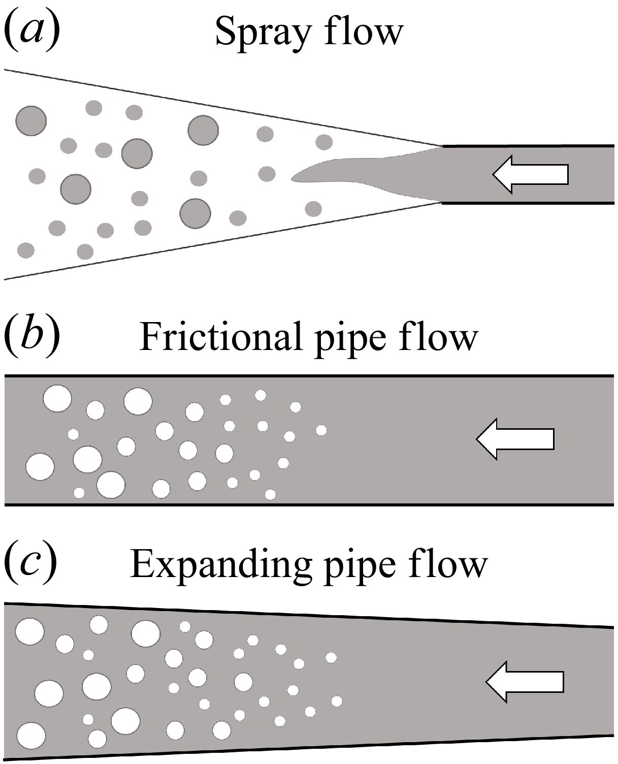

 P−ρ


 Γ


 ceq
 cW


 ceq
 cη (η=0.3)
 cW
 ceq

 ceq
 cη (η=0.3)
 cW
 ceq

 ceq
 cη (η=0.3)
 cW
 ceq





