1 Introduction
Due to the rapid growth of civil air traffic and ambitious goals for the reduction of pollutant emissions, the development of eco-efficient aircraft requires elaborate fuel saving technologies. Laminar flow control (LFC) on wings and tail empennage offers a great potential to decrease the overall drag and has lately gained attention due to test campaigns and even implementation of large-scale production by leading aircraft manufacturers. Promising efforts rely on approaches such as leading-edge suction or natural laminar flow. Such methods delay the transition to turbulent flow, but their capability to relaminarise an already turbulent boundary layer is limited. Accordingly, premature transition due to surface imperfections such as discrete roughness elements has to be prevented and is therefore a scenario of great practical importance.
Since the 1950s, numerous publications have been dedicated to investigating the near-field flow structures of isolated roughness elements in two-dimensional boundary layers, and finding the criteria for a ‘critical’ roughness, triggering transition to turbulence immediately; an overview is given below. While most investigations were and still are devoted to the transition-promoting effect of roughness elements in two-dimensional symmetric boundary layers, the swept-back wings of modern aircraft produce a three-dimensional boundary-layer profile characterised by cross-flow instability, especially in the leading-edge region. In the present work, we address the validity of existing studies for a three-dimensional base flow as present on an infinite swept wing.
For two-dimensional boundary layers, Gregory & Walker (Reference Gregory and Walker1956) published one of the first systematic investigations of discrete, cylindrical roughness elements and their effect on transition. They identified a steady horseshoe vortex in front of, and spiral vortices behind, the elements. When reaching a certain roughness height, the latter broke down and gave rise to periodic vortex shedding, ultimately leading to turbulent flow. While for modest roughness size the flow downstream appeared almost unaffected, the emergence of a turbulent wedge was found to occur rather abruptly when a critical roughness height was reached. Together with the work by Klanfer & Owen (Reference Klanfer and Owen1953), a Reynolds number
 $Re_{kk,crit}$
based on the roughness height and the downstream velocity of the undisturbed flow at the position of the tip of the roughness was found to be the best measure to describe the effect of the element on the boundary layer. Following studies by Mochizuki (Reference Mochizuki1961), Tani (Reference Tani1961) and Tani et al. (Reference Tani, Komoda, Komatsu and Iuchi1962) also addressed the influence of free-stream turbulence and the pressure gradient. Von Doenhoff & Braslow (Reference Von Doenhoff and Braslow1961) collected published data and found that
 $Re_{kk,crit}$
increases with the aspect ratio
 $r_{a}=k/d$
, with
 $k$
being the roughness height and
 $d$
the roughness diameter. For spanwise oriented roughness arrays they found that the spacing between the elements is only a relevant parameter for values below three times the roughness diameter – for larger spacing, the roughness elements can be treated as isolated. Sedney (Reference Sedney1973) compiled a survey of the findings in the 1950s and 1960s.
A closer look on the near-field flow structures around isolated roughness elements was undertaken by Baker (Reference Baker1979) in an investigation of the formation of horseshoe vortices. Kendall (Reference Kendall1981) classified the downstream disturbance evolution behind a roughness element into a near wake, where the velocity deficit due to the recirculation zone dominates, and a far wake dominated by the vertical displacement of streamwise momentum as an effect of the streamwise legs of the horseshoe-vortex system. Acarlar & Smith (Reference Acarlar and Smith1987) conducted extensive water-tunnel measurements of the flow past a hemispherical roughness element. They again found a horseshoe vortex, but focused on the role of unsteady hairpin vortices in the roughness-promoted transition process and attributed a key role to these structures. Klebanoff, Cleveland & Tidstrom (Reference Klebanoff, Cleveland and Tidstrom1992) addressed the strong inflectional velocity profiles in the near wake and found a correlation with the wall-normal maxima of the velocity fluctuations. When the latter reached nonlinear amplitudes, rapid transition to turbulent flow was observed.
For roughness elements with subcritical height, low-speed streaks form due to the lift-up effect (Landahl Reference Landahl1980) as the boundary layer develops downstream. One of the first results indicating transient growth behind isolated roughness elements was reported by Gaster, Grosch & Jackson (Reference Gaster, Grosch and Jackson1994). For a series of experiments with a shallow oscillating bump, they observed the growth of a spanwise disturbance mode that could not be explained by linear theories. Accompanying simulations by Joslin & Grosch (Reference Joslin and Grosch1995) qualitatively confirmed the findings and detected a pair of counter-rotating streamwise vortices evolving to the sides of the bump, causing a low-speed-streak growth in the downstream centreline by the lift-up effect. A series of experiments aimed at the understanding of roughness-induced transient growth was conducted by, e.g. White & Ergin (Reference White and Ergin2003), Ergin & White (Reference Ergin and White2005, Reference Ergin and White2006), Denissen & White (Reference Denissen and White2008); the major findings are compiled in White (Reference White2005). White & Ergin (Reference White and Ergin2003) observed that the energy associated with transiently amplified disturbances scales with
 $Re_{kk}^{2}$
for roughness elements. Direct numerical simulations (DNS) by Fischer & Choudhari (Reference Fischer and Choudhari2004) and Choudhari & Fischer (Reference Choudhari and Fischer2005), mimicking the experimental set-up, confirmed this empirical rule up to at least
 $Re_{kk}\approx 250$
, and also addressed effects of roughness shape and spacing. All observed transient disturbances, however, are found to be ‘suboptimal’, i.e. all experimentally and numerically observed amplitude ratios are far below what is predicted by optimal disturbance theory (see Andersson, Berggren & Henningson Reference Andersson, Berggren and Henningson1999; Luchini Reference Luchini2000; Tumin & Reshotko Reference Tumin and Reshotko2001). Consequently, Choudhari & Fischer (Reference Choudhari and Fischer2005) state that the relevance of transient streak growth caused by decaying symmetrical vortex pairs for roughness-induced transition is questionable. Rather, again periodic vortex shedding set in at a certain roughness height,
 $Re_{kk}=435$
, in their simulations.
Measurements of unsteady velocity fluctuations by Ergin & White (Reference Ergin and White2006) showed a correlation of fluctuation maxima and inflection points in the downstream velocity component of the time-averaged flow. The dominant frequency band compared well with results from a simple model for the Kelvin–Helmholtz instability. Therefore, the earlier findings by Klebanoff et al. (Reference Klebanoff, Cleveland and Tidstrom1992) were substantiated, making clear that transient growth is not involved in the near-field turbulence-tripping mechanism by discrete roughness elements.
DNS with roughness elements employing an overset-grid approach were performed by Rizzetta & Visbal (Reference Rizzetta and Visbal2007). The cylindrical roughness elements were meshed by a cylindrical mesh embedded in a Cartesian background grid block. The flow under consideration and the roughness geometry were adopted from Ergin & White (Reference Ergin and White2006). Time-mean streamwise-velocity contours match experimental results by, e.g. Denissen & White (Reference Denissen and White2008). A subcritical roughness configuration revealed the existence of a system of two horseshoe vortices. For a critical roughness element, velocity fluctuations corresponding to inflection points in the time-mean velocity contours were correlated with the emergence of hairpin vortex shedding, leading to rapid transition.
Another series of DNS intended to reproduce the results by Ergin & White (Reference Ergin and White2006) was performed by Stephani & Goldstein (Reference Stephani and Goldstein2009), Drews et al. (Reference Drews, Downs, Doolittle, Goldstein and White2011) and Doolittle, Drews & Goldstein (Reference Doolittle, Drews and Goldstein2014). The cylindrical roughness elements were modelled by an immersed boundary method, imposing the no-slip condition on specified grid points. The resulting shape was consequently jagged, and the series of investigations shows a non-negligible resolution dependence. The simulations by Doolittle et al. (Reference Doolittle, Drews and Goldstein2014) further addressed the formation of horseshoe vortices in front of the roughness and found good agreement with the systematic investigation by Baker (Reference Baker1979). Zhou, Wang & Fan (Reference Zhou, Wang and Fan2010) simulated the flow past a hemispherical roughness element and compared their results with Klebanoff et al. (Reference Klebanoff, Cleveland and Tidstrom1992). Quantitative differences in the wall-normal distribution of the downstream velocity fluctuations are attributed to different incoming turbulence levels. In the simulations, these fluctuations could be linked to the existence of hairpin vortices.
Bernardini, Pirozzoli & Orlandi (Reference Bernardini, Pirozzoli and Orlandi2012), Bernardini et al. (Reference Bernardini, Pirozzoli, Orlandi and Lele2014) also conducted a DNS series on a set-up mimicking the conditions of Ergin & White (Reference Ergin and White2006). They spanned a wide parameter space by varying parameters of the oncoming flow and the roughness geometry. Based on this data base, a turbulence-tripping criterion taking the blocked mass flux into account was derived, scaling out the influence of Mach number and roughness shape.
Stability analyses of the highly three-dimensional flow in the near wake of roughness elements have been performed by different approaches, see Theofilis (Reference Theofilis2011) for a review on topical stability analysis methods. Biglobal stability analysis to investigate roughness wakes in planes perpendicular to the main flow was mainly used in supersonic boundary layers, see, e.g. Groskopf, Kloker & Marxen (Reference Groskopf, Kloker, Marxen, Schlatter and Henningson2010); recent studies for subsonic boundary-layer flow are reported by Denissen & White (Reference Denissen and White2013) and Shin, Rist & Krämer (Reference Shin, Rist and Krämer2015). The two-dimensional unstable eigenfunctions were either of varicose or sinuous type, where a dominant varicose mode could be connected to the three-dimensional shear layer developing downstream of the roughness.
Loiseau et al. (Reference Loiseau, Robinet, Cherubini and Leriche2014) performed an extensive investigation of the global stability of a configuration adopted from the turbulence-tripping case in the experiments by Fransson et al. (Reference Fransson, Brandt, Talamelli and Cossu2005). Based on a comparison with the experimental data, the authors find the flow tripping by the roughness to be connected to a global instability of the flow field. By varying the aspect ratio
 $r_{a}=k/d$
of the cylindrical roughness element, two mechanisms acting as a wavemaker, the core of the absolute instability, could be identified. First, for
 $r_{a}<1$
, the wavemaker has a varicose appearance and is located in the shear layer evolving from the top of the roughness. This scenario most likely corresponds to the observations made in previous studies. Second, for
 $r_{a}\geqslant 1$
, an antisymmetric wavemaker similar to the generator of a von Kármán vortex street is present in the shear layers emanating from the lateral edges of the roughness. Although an antisymmetric modulation is found in an accompanying unsteady nonlinear DNS, the transition process appears to be dominated by almost symmetric hairpin vortices. The reason for this observation remains unclear.
Investigations of the flow past discrete roughness elements in three-dimensional swept-wing boundary layers are scarce and mainly concentrate on micron-sized roughness elements that are in the so-called ‘linear’ range of receptivity, where a surface imperfection induces a characteristic local disturbance flow field that may be superposed on the base flow. Note, however, that the strength of the disturbance flow field may depend nonlinearly on roughness parameters such as as the height, as shown by Luchini (Reference Luchini2013) for a generic boundary layer and Choudhari & Duck (Reference Choudhari and Duck1996) and Kurz & Kloker (Reference Kurz and Kloker2014b ) for swept-wing flow. In the presence of cross-flow instability, such shallow roughness elements induce unstable steady cross-flow modes; a review on related receptivity studies is given in Kurz & Kloker (Reference Kurz and Kloker2014b ). A practical application in the scope of LFC is the stabilisation of a three-dimensional boundary layer by the induction of a control mode, as suggested by Saric, Carrillo & Reibert (Reference Saric, Carrillo and Reibert1998) and the recent associated DNS by Hosseini et al. (Reference Hosseini, Tempelmann, Hanifi and Henningson2013); see also the detailed simulations by Wassermann & Kloker (Reference Wassermann and Kloker2002).
The flow past a spanwise-periodic array of roughness elements having a height of approximately 30 % of the local displacement thickness was computed by Piot, Casalis & Terracol (Reference Piot, Casalis and Terracol2007). Due to the short simulation time, the flow downstream of the roughness array comprised steady cross-flow modes and slowly decaying travelling cross-flow waves, the latter resulting from the sudden introduction of the roughness elements into the undisturbed base state at the beginning of the simulation. A saddle-point analysis presented in Piot & Casalis (Reference Piot and Casalis2009) shows that the observed unsteady modes are indeed damped. Further, Piot & Casalis (Reference Piot and Casalis2009) again point out that a decay may be counteracted by an undue pressure feedback from the outflow boundary condition, as has been discussed by Buell & Huerre (Reference Buell and Huerre1988) and Kloker, Konzelmann & Fasel (Reference Kloker, Konzelmann and Fasel1993).
Larger roughness elements with heights of the order of the local displacement thickness still induce high-amplitude cross-flow vortices invoking (convective) secondary instability shortly downstream, but the flow in the vicinity of the roughness becomes more complex due to the formation of steady vortex systems and a recirculation region. DNS with a spanwise array of such roughnesses were performed by Brynjell-Rahkola et al. (Reference Brynjell-Rahkola, Schlatter, Hanifi and Henningson2015) who also presented preliminary results from a global stability analysis. DNS by Kurz & Kloker (Reference Kurz, Kloker and Dillmann2014a ) showed that disturbance growth in the near wake may directly contaminate the flow by unsteady vortex shedding; the analogies to a respective two-dimensional boundary-layer case are highlighted in Kurz & Kloker (Reference Kurz, Kloker and Nagel2015b ). As observed by Kurz & Kloker (Reference Kurz and Kloker2015a ), this scenario may be promoted by either a strong convective or a global instability caused by the recirculation zone in the near wake of the roughness element.
In the present work, we compare a subcritical roughness case in the three-dimensional swept-wing flow to a respective two-dimensional base-flow case, before we focus on the three-dimensional case. The roughness height is increased, and the background disturbance level is varied in order to find the critical roughness Reynolds number
 $Re_{kk,crit}$
. For a quasi-critical and distinctly over-critical
 $Re_{kk}$
, we investigate the temporal evolution of unsteady disturbances starting from an artificial steady solution, in order to characterise the nature of the dominant instability mechanism. Finally, global stability analyses of these two cases are performed.
2 Numerical method
All data presented in the present investigation are based on DNS. In order to observe the temporal disturbance growth for near-critical roughness elements, we employ various numerical techniques in our compressible flow solver.
2.1 Direct numerical simulations
DNS are performed using a sixth-order accurate, compact finite-difference flow solver, solving the time-dependent, three-dimensional, compressible Navier–Stokes equations in non-dimensional conservative formulation. Time integration is accomplished by an explicit fourth-order Runge–Kutta scheme. Details on the simulation code, the base-flow computation as well as the numerical set-up including the representation of the roughness and the boundary conditions can be found in Kurz & Kloker (Reference Kurz and Kloker2014b ) and are summarized briefly below.
The base flow past a swept wing with infinite span is computed by the Reynolds-averaged Navier–Stokes (RANS) solver TAU with second-order accuracy. The laminar solution in the front part of the wing is transferred to a structured high-resolution DNS grid by a high-order Lagrangian interpolation and further converged in two steps by a two-dimensional DNS. For the three-dimensional unsteady DNS we use characteristic boundary conditions at inflow boundary, free-stream boundary and outflow boundary in conjunction with sponge layers based on a volume-forcing term. Further, the computational grid is stretched perpendicular to the wall and in the downstream direction in front of the outflow boundary to eliminate high-wavenumber disturbances in conjunction with a tenth-order compact spatial filter. At the wall we impose the no-slip condition, an isothermal formulation keeping the adiabatic wall temperature of the base flow without roughness and a pressure extrapolation from the domain interior.
2.2 Selective frequency damping
Artificial steady solutions of globally unstable flows are obtained with our DNS code employing the method called selective frequency damping (SFD), see Akervik et al. (Reference Akervik, Brandt, Henningson, Hoepffner, Marxen and Schlatter2006). This is realized by adding a source term to the right-hand side of the Navier–Stokes equations, acting as a temporal filter,
 $$\begin{eqnarray}\frac{\partial \boldsymbol{Q}}{\partial t}=\left.\frac{\partial \boldsymbol{Q}}{\partial t}\right|_{Navier{-}Stokes}-{\it\chi}(\unicode[STIX]{x1D644}-T)\boldsymbol{Q},\end{eqnarray}$$
with the vector of the conservative variables
 $\boldsymbol{Q}$
, time
 $t$
, gain factor
 ${\it\chi}$
, temporal filter kernel
 $T$
and identity matrix
 $\unicode[STIX]{x1D644}$
. As the solution converges towards a steady state, the filter term vanishes
 $(\unicode[STIX]{x1D644}\rightarrow T)$
, leaving a solution of the unmodified Navier–Stokes equations.
2.3 Nonlinear disturbance formulation
In practice, the SFD source term will never be exactly zero, but has a small finite value. Hence, if the SFD is simply switched off to observe the (linear) temporal evolution of the flow starting from the steady state, there is a small pulse-like temporal discontinuity due to the sudden removal of the filter term. Instead, we employ a nonlinear disturbance formulation for the temporal evolution simulations, where the temporal derivative of the state at the last time step of the damped simulation,
 $\boldsymbol{Q}_{0}$
, is forced to zero by subtracting the ‘base-flow derivative’
 $$\begin{eqnarray}\frac{\partial \boldsymbol{Q}}{\partial t}=\left.\frac{\partial \boldsymbol{Q}}{\partial t}\right|_{Navier{-}Stokes}-\frac{\partial \boldsymbol{Q}_{0}}{\partial t}.\end{eqnarray}$$
Thereby, the passage from the SFD steady state to the unsteady DNS is smoothed. Although the small source term is kept, the temporal damping effect is switched off immediately, since there is no further adjustment of it to numerical background noise or incoming disturbances in the flow.
2.4 Global stability analysis
The stability analysis of the compressible, fully three-dimensional flow field around the roughness element is defined by the global mode ansatz
 $$\begin{eqnarray}\boldsymbol{q}^{\prime }(\boldsymbol{x},t)=\hat{\boldsymbol{q}}(\boldsymbol{x})\text{e}^{-\text{i}{\it\omega}t}+\text{c.c.},\end{eqnarray}$$
with perturbation state vector
 $\boldsymbol{q}^{\prime }$
and the complex eigenfunction
 $\hat{\boldsymbol{q}}=(\hat{\boldsymbol{u}},\hat{\boldsymbol{v}},\hat{\boldsymbol{w}},\hat{{\bf\rho}},\hat{\boldsymbol{T}})^{\text{T}}$
, position vector
 $\boldsymbol{x}$
,
 $\text{i}=\sqrt{-1}$
and angular frequency
 ${\it\omega}\in \mathbb{C}$
; for an overview of global linear stability analysis, see Theofilis (Reference Theofilis2011). In order to solve the associated eigenvalue problem, the compressible Navier–Stokes equations in disturbance formulation were linearised around a steady-state solution by cancellation of higher-order disturbance terms. Thus, we can write
 $$\begin{eqnarray}\frac{\partial \boldsymbol{q}^{\prime }}{\partial t}=\unicode[STIX]{x1D647}\boldsymbol{q}^{\prime },\end{eqnarray}$$
with the discrete linearised Navier–Stokes operator
 $\unicode[STIX]{x1D647}$
, being represented by an
 $n\times n$
– matrix. The associated eigenvalue problem is defined as
 $$\begin{eqnarray}\unicode[STIX]{x1D647}\hat{\boldsymbol{q}}={\it\lambda}\hat{\boldsymbol{q}},\end{eqnarray}$$
with the eigenvalues
 ${\it\lambda}_{j}=-\text{i}{\it\omega}_{j}$
and eigenvectors
 $\hat{\boldsymbol{q}}_{j}$
of the system matrix. The dimension of the system is
 $n=5N_{{\it\xi}}N_{{\it\eta}}N_{z}=O(10^{8})$
in the present case, where
 $N_{{\it\xi}}$
,
 $N_{{\it\eta}}$
,
 $N_{z}$
are the number of grid points in chordwise, wall-normal and spanwise directions, respectively. Although modern iterative Krylov-subspace methods are capable of tackling large eigenvalue problems,
 $\unicode[STIX]{x1D647}$
is simply too large to be stored explicitly in main memory, even on state-of-the-art super computers. Therefore, we employ a matrix-free time-stepper approach as proposed by Edwards et al. (Reference Edwards, Tuckerman, Friesner and Sorensen1994), and used for complex flows by, among others, Barkley, Gomes & Henderson (Reference Barkley, Gomes and Henderson2002), Bagheri et al. (Reference Bagheri, Schlatter, Schmid and Henningson2009) and recently Loiseau et al. (Reference Loiseau, Robinet, Cherubini and Leriche2014). For that purpose, the transformed eigenvalue problem
 $$\begin{eqnarray}\text{e}^{\unicode[STIX]{x1D647}{\rm\Delta}t}\hat{\boldsymbol{q}}={\it\sigma}\hat{\boldsymbol{q}},\end{eqnarray}$$
with the fixed time interval
 ${\rm\Delta}t$
and the transformed eigenvalues
 ${\it\sigma}_{j}$
is solved by a matrix-free Rayleigh–Ritz method based on a Krylov subspace. We employ the Krylov–Schur method implemented in the software library SLEPc (Hernandez, Roman & Vidal Reference Hernandez, Roman and Vidal2005), an algorithm similar to the classical Arnoldi iteration with an effective restarting procedure, developed by Stewart (Reference Stewart2002). In this work, we use
 ${\rm\Delta}t=1.277\times 10^{-4}$
, corresponding to 300 time steps of the Navier–Stokes solver, a subspace dimension of 480 and a convergence criterion for the eigenvalues of
 $10^{-8}$
.
3 Flow configuration
The flow under consideration is characterised by generic jet-transport-aircraft free-stream conditions and the wing profile defined in the European Commission FP7 project ‘RECEPT’.
3.1 Base flow
We consider the compressible boundary-layer flow over a modified laminar NACA
 $67_{1}-215$
profile with infinite span. The chord length perpendicular to the leading edge is
 $\bar{L}=2.0~\text{m}$
(the overbar denotes dimensional values) serving as reference length for non-dimensionalisation of the wall-parallel coordinates, whereas all other length scales are related to the displacement thickness (in compressible formulation) in the streamline-oriented coordinate system,
 $\bar{{\it\delta}}_{1,s,R}=1.7\times 10^{-4}~\text{m}$
, evaluated at the downstream position of the roughness,
 $x_{R}=0.02$
. The sweep angle is
 ${\it\beta}_{\measuredangle }=35^{\circ }$
and the angle of attack measured in a plane perpendicular to the leading edge is
 ${\it\alpha}_{\measuredangle }=-6.1^{\circ }$
.
A steady reference solution is computed with the Reynolds-averaged Navier–Stokes (RANS) solver TAU with fixed transition at
 $x_{tr}=0.2$
on both upper and lower sides. The free-stream velocity magnitude
 $\bar{Q}_{\infty }=191.8~\text{m}~\text{s}^{-1}$
serves as reference value for non-dimensionalisation of all velocity components; the chordwise and spanwise velocity components are
 $\bar{U}_{\infty }=157.1~\text{m}~\text{s}^{-1}$
and
 $\bar{W}_{\infty }=110.0~\text{m}~\text{s}^{-1}$
, respectively. The flow is further characterised by
 $Ma_{\infty }=\bar{Q}_{\infty }/\bar{a}_{\infty }=0.65$
, where
 $\bar{a}_{\infty }$
is the free-stream speed of sound, and
 $Re_{Q}=\bar{Q}_{\infty }\bar{{\it\rho}}_{\infty }(\bar{L}/\cos {\it\beta}_{\measuredangle })/\bar{{\it\mu}}_{\infty }=10.3\times 10^{6}$
, with free-stream values of the density
 $\bar{{\it\rho}}_{\infty }$
and dynamic viscosity
 $\bar{{\it\mu}}_{\infty }$
. The resulting flow on the considered upper wing side has a stagnation line at
 $x=0.01$
and subsequent acceleration up to
 $x=0.7$
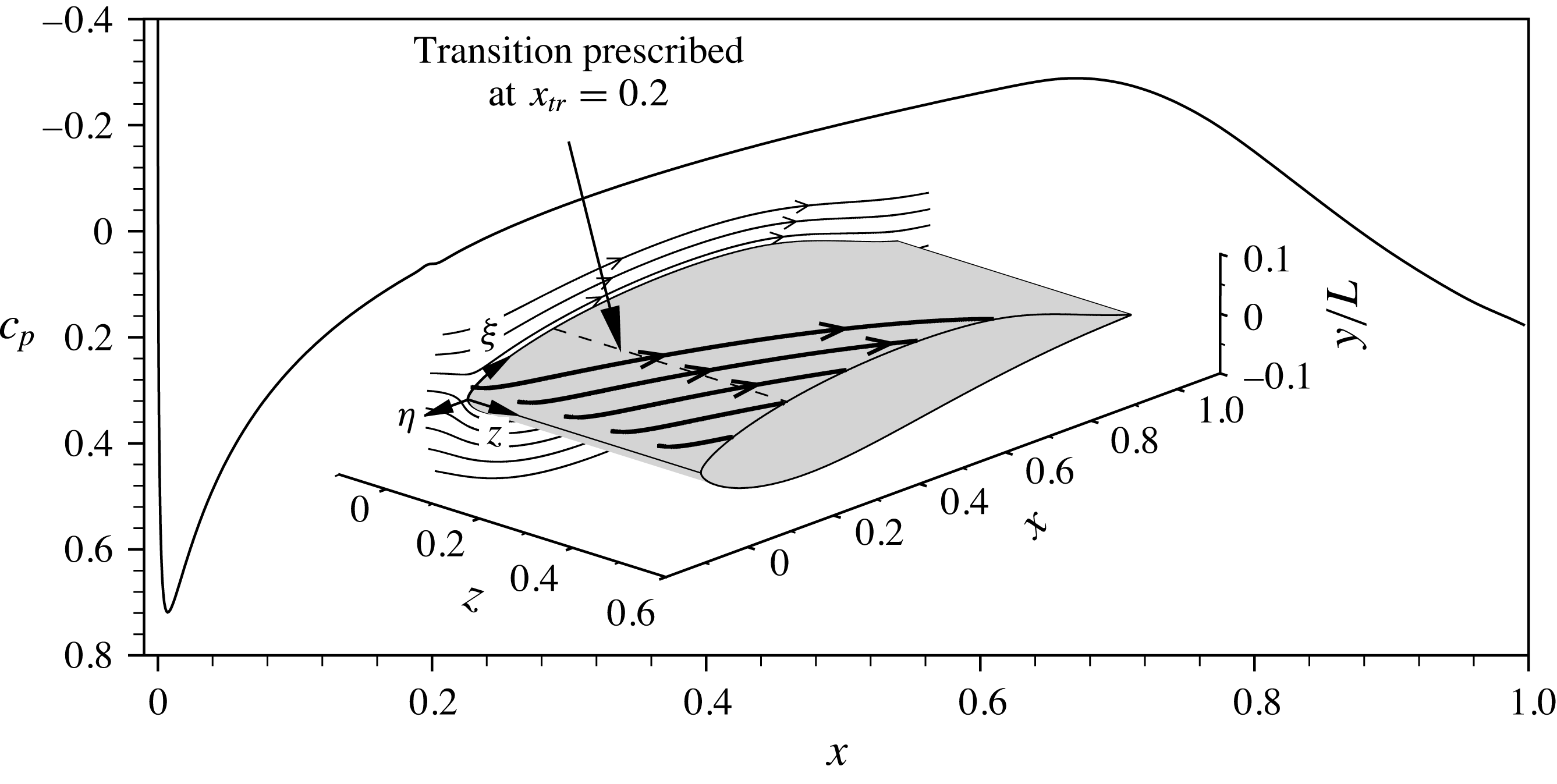
. The distribution of the pressure coefficient
 $c_{p}=(p-p_{\infty })/(0.5{\it\rho}_{\infty }Q_{\infty }^{2})$
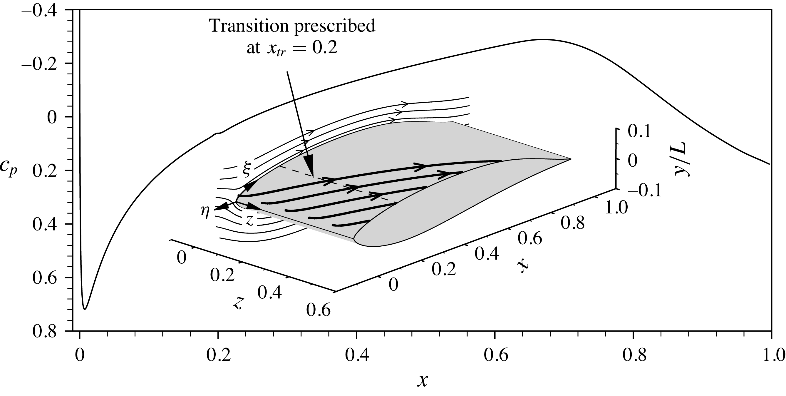
on the upper wing side is given in figure 1. For details on the stability properties and boundary-layer parameters, see Kurz & Kloker (Reference Kurz and Kloker2014b
).
Distribution of the pressure coefficient
 $c_{p}$
on the upper side of the swept-wing profile. The inset shows two-dimensional streamlines (thin, spanwise velocity component
 $w$
set to zero) and three-dimensional streamlines (thick), the latter starting close to the boundary-layer edge in the stagnation-line region. The dashed line depicts the prescribed transition location
 $x_{tr}=0.2$
for the base-flow computation. The curvilinear tangential system
 $({\it\xi},{\it\eta},z)$
has its origin at the leading edge.
The numerical domain
 ${\it\Omega}_{1}$
used for the DNS is spanned by a structured grid with a downstream extent
 $0.015<x<0.0325$
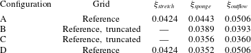
and uniformly spaced grid points along the wall, cf. figure 2 and table 1. The domain is extended in downstream direction by a stretched outflow zone up to
 $x=0.0454$
, cf. § 2.1. The domain height is
 ${\it\eta}_{max}=333\times {\it\delta}_{1,s,R}$
, whereas the wall-normal point distribution is relaxed by a variable stretching factor in
 ${\it\eta}$
-direction, i.e.
 ${\it\chi}_{{\it\eta},bl}$
in the boundary-layer region and
 ${\it\chi}_{{\it\eta}}$
above. The periodic
 $z$
-direction has an extent of
 ${\it\lambda}_{z,0}/{\it\delta}_{1,s,R}=23.52$
, corresponding to the wavelength of the most unstable steady cross-flow mode. Note that the spanwise wavelength leading to the local maximum amplification rate and the wavelength first reaching the transition
 $N$
-factor
 $N=9$
almost coincide. This reference grid has a total resolution of
 $N_{{\it\xi}}\times N_{{\it\eta}}\times N_{z}=1258\times 188\times 128=30\times 10^{6}$
points.
Parameters for the reference grids and the high-resolution grid used for a resolution study. The reference length for the two-dimensional grid is
 $\bar{{\it\delta}}_{1,R,2D}=2.07\times 10^{-4}~\text{m}$
, for the other grids it is
 $\bar{{\it\delta}}_{1,s,R}=1.7\times 10^{-4}~\text{m}$
. For definitions, see § 3.1.

DNS set-up on the reference grid; the stretched outflow zone is truncated. For clarity, two, ten and eight grid lines are skipped in wall-parallel, downstream and spanwise directions, respectively. The disturbance strip is located at
 $x=0.018$
, the roughness at
 $x_{R}=0.02$
. Base-flow streamlines are given at various (i) wall-normal positions in the boundary layer and (ii) downstream positions along the boundary-layer edge. The inset shows a roughness with height
 $k=1.5$
in full resolution.

For a resolution study, we use a numerical grid where the step sizes in all three directions are reduced by approximately
 $\sqrt{2}$
, see table 1 for the exact values. The total number of grid points for this high-resolution grid is
 $1764\times 256\times 168=76\times 10^{6}$
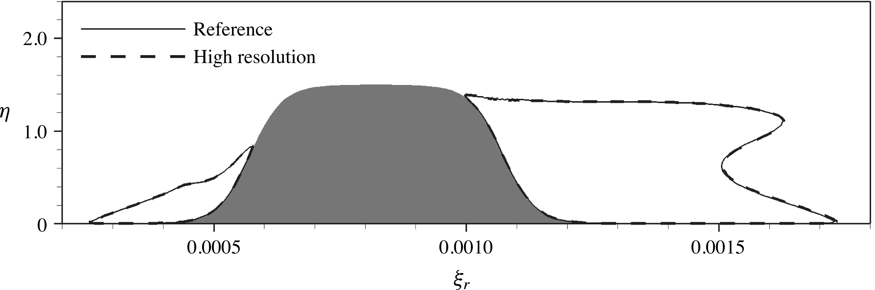
. Figure 3 shows the recirculation zones developing upstream and downstream of a roughness element with a height of
 $1.5\times {\it\delta}_{1,s,R}$
, cf. § 3.3. For both the reference and the high-resolution grid, the shapes of the reversed flow regions are in excellent agreement. High-resolution results for the nonlinear, unsteady disturbance evolution downstream of the same roughness elements are given in figures 8(d) and 9(b), again showing good agreement with the respective data obtained on the reference grid. Therefore, the use of the reference grid for all our simulations is justified.
Regions of reversed flow in a cross-cut through the centre of a roughness with
 $k=1.5,Re_{kk}=564$
, marked by contours of
 $u_{r}=-1\times 10^{-4}$
, for two grid resolutions. The
 ${\it\eta}$
-axis is stretched by a factor of 2 for clarity.

For comparison, we define a two-dimensional base flow on the same wing geometry by omitting the spanwise velocity component in the oncoming free stream. This results in a comparable chordwise boundary-layer thickness as in the three-dimensional case. With the modified free-stream conditions, we obtain
 $Ma_{\infty ,2D}=0.53$
and
 $Re_{U,2D}=6.9\times 10^{6}$
. The flow is again computed with TAU, table 1 gives the associated grid parameters for the DNS. The reference length for all two-dimensional results shown within this study is the displacement thickness
 $\bar{{\it\delta}}_{1,R,2D}=2.07\times 10^{-4}~\text{m}$
, corresponding to roughness position
 $x_{R,2D}=0.06$
. The reference velocity for the two-dimensional case is
 $\bar{U}_{\infty }=157.1~\text{m}~\text{s}^{-1}$
.
3.2 Coordinate systems
We use four different coordinate systems for the simulations and evaluation. In the Cartesian global coordinate system
 $(x,y,z)$
, as used in the DNS,
 $x$
is aligned with the shortest distance between leading and trailing edge,
 $y$
points upwards and
 $z$
is parallel to the leading edge, cf. figure 2. The origin collapses with the leading edge. The associated velocity components are denoted
 $(u_{g},v_{g},w_{g})$
.
The tangential coordinate system
 $({\it\xi},{\it\eta},z)$
, depicted in figure 1, with velocity components
 $(u,v,w)$
, is of curvilinear type and has the same origin and the identical spanwise coordinate
 $z$
, while
 ${\it\xi}$
runs perpendicular to the leading edge along the upper profile surface and
 ${\it\eta}$
is defined to be the wall-normal direction everywhere. When plotting this system on a Cartesian grid, the flow field is slightly distorted and the surface appears flat.
Based on the tangential system, the flow field may be further transformed to a rotated coordinate system
 $({\it\xi}_{r},{\it\eta},z_{r})$
with velocity components
 $(u_{r},v,w_{r})$
for visualisation purposes. The origin is shifted to the centre of a roughness element. Therefore, the flow field is rotated about the
 ${\it\eta}$
axis by the arbitrarily chosen angle
 ${\it\phi}_{r}=55^{\circ }$
so as to be aligned with the steady cross-flow vortices. For cases in the two-dimensional boundary layer, we choose
 ${\it\phi}_{r}=0^{\circ }$
, that is, only the origin is shifted compared to the tangential system.
The fourth coordinate system
 $({\it\xi}_{s},{\it\eta},z_{s})$
is closely related to the
 $r$
-system, but its first coordinate is locally aligned with the projection of the boundary-layer edge velocity vector to the surface. The respective velocity components are
 $(u_{s},v,w_{s})$
. In particular,
 $u_{s}$
is evaluated in order to measure the downstream development of boundary-layer disturbances.
3.3 Roughness elements
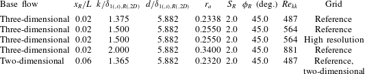
The roughness elements are represented by a smoothed circular disk as illustrated in the inset in figure 2, with the shape of the shoulders being defined by a hyperbolic tangent function, cf., e.g. Kurz & Kloker (Reference Kurz and Kloker2014b ). The latter is defined in polar coordinates
 $$\begin{eqnarray}{\it\eta}_{R}(r,{\it\phi})=\frac{k}{2}\left\{\tanh \left[\frac{S_{R}}{k}\left(\frac{d}{2}-r\right)\right]+1\right\}\!,\quad r\geqslant 0,0\leqslant {\it\phi}<2{\rm\pi},\end{eqnarray}$$
with
 $k$
and
 $d={\it\lambda}_{z,0}/4$
being the nominal height and diameter, respectively, also defining the aspect ratio
 $r_{a}=k/d$
, the slope factor
 $S_{R}$
and the maximum slope angle
 ${\it\phi}_{R}$
. In the three-dimensional case, the roughness centre is placed at
 $x_{R}=0.02$
,
 ${\it\xi}_{R}=0.0285$
,
 $Re_{{\it\delta}1,s,R}=500$
; in the two-dimensional case, it is centred at
 $x_{R,2D}=0.06$
,
 ${\it\xi}_{R,2D}=0.0718$
,
 $Re_{{\it\delta}1,R,2D}=499$
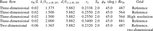
. All roughness elements considered in this work are listed in table 2. Note that smooth roughness shapes lead to a somewhat less transition-critical behaviour than sharp elements, as indicated in a recent investigation by Loiseau et al. (Reference Loiseau, Cherubini, Robinet and Leriche2015).
The effect of the elements on the boundary-layer flow is characterised by the roughness Reynolds number based on the height and the velocity magnitude in the undisturbed base flow corresponding to the position of the roughness tip:
 $$\begin{eqnarray}Re_{kk}=\frac{|\bar{\boldsymbol{u}}(\bar{k})|\bar{k}\bar{{\it\rho}}(\bar{k})}{\bar{{\it\mu}}(\bar{k})},\end{eqnarray}$$
with
 $\boldsymbol{u}=(u,v,w)^{\text{T}}$
. Note that
 $\bar{\boldsymbol{u}}$
may be not exactly parallel to the wall.
Shape and flow parameters of investigated roughness configurations. For three-dimensional base flows, the reference length is
 $\bar{{\it\delta}}_{1,s,R}=1.7\times 10^{-4}~\text{m}$
, for the two-dimensional base flow we use
 $\bar{{\it\delta}}_{1,R,2D}=2.07\times 10^{-4}~\text{m}$
. For further definitions, see § 3.3.
In the DNS, the smooth roughness elements are introduced by a local elevation of wall grid points, compressing the wall-parallel mesh layers within a defined height above the roughness. The wall-normal grid lines keep their orientation.
3.4 Disturbance source
In order to control the level of background disturbances in the boundary layer, we introduce controlled disturbances by a spatially confined, time-harmonic blowing and suction strip at the wall, its centre being located upstream of the roughness element at
 $x=0.0178$
,
 ${\it\xi}=0.0260$
, see figure 2. The vertical mass flux
 $({\it\rho}v_{g})_{dist}$
through the disturbance strip follows the distribution function
 $$\begin{eqnarray}({\it\rho}v_{g})_{dist}=\hat{A}\underbrace{\sin ({\rm\pi}x^{\ast })\text{e}^{-({\rm\pi}x^{\ast })^{2}/\sqrt{2}}\cos ({\it\gamma}_{0}z)}_{D_{s}}\underbrace{\frac{1}{50}\mathop{\sum }_{h=1}^{50}\cos (h{\it\omega}_{0}t)}_{D_{t}},\quad x^{\ast }\in [-1;1],\end{eqnarray}$$
with the amplitude
 $\hat{A}$
, which was set to
 $2.5\times 10^{-3}$
for the low-noise set-up and to
 $2.5\times 10^{-2}$
for the high-noise set-up; the spatial and temporal modulations are denoted
 $D_{s}$
and
 $D_{t}$
, respectively. The normalised downstream coordinate
 $x^{\ast }$
corresponds to the physical range
 $0.0176<x<0.0181$
and
 $0.0258<{\it\xi}<0.0263$
, respectively. Multiples
 $h$
of the fundamental angular frequency
 ${\it\omega}_{0}=328$
are prescribed, where
 ${\it\omega}_{0}$
is close to the frequency of the most amplified cross-flow wave. The fundamental spanwise wavenumber
 ${\it\gamma}_{0}=2{\rm\pi}/{\it\lambda}_{z,0}$
conforms to the locally and integrally most amplified steady cross-flow mode. We superpose frequencies with
 $h=1{-}50$
, producing periodic disturbance pulses; in the initial phase, the disturbance is ramped up.
4 Steady vortex system and recirculation zone
First, we compare the steady vortex systems forming around a subcritical roughness in both a two-dimensional and a three-dimensional boundary layer. The element in the former case has a height of
 $k=1.365$
,
 $Re_{kk}=487$
and is placed at
 $x_{R,2D}=0.06$
, where the local Reynolds number
 $Re_{{\it\delta}1,R,2D}$
is identical to the respective value in direction of the local edge velocity
 $Re_{{\it\delta}1,s,R}$
in the three-dimensional case, cf. § 3.3. Note that the associated shape factors, based on the incompressible displacement and momentum thickness, are
 $H_{12,inc,2D}=2.31$
and
 $H_{12,s,inc}=2.47$
for the two-dimensional and the three-dimensional cases, respectively.
Near-field vortex systems with inner vortex pairs (IV) and horseshoe-vortex legs (HV), induced by discrete roughness elements: (a) two-dimensional base flow,
 $k=1.365$
,
 $Re_{kk}=487$
, (b) three-dimensional base flow,
 $k=1.375$
,
 $Re_{kk}=487$
, with streamlines of the base state without roughness. Vortices are visualised by isosurfaces at
 ${\it\lambda}_{2}^{\ast }=-2.0\times 10^{-4}$
, structures above roughness elements are blanked. The shading indicates positive and negative values of
 ${\it\omega}_{{\it\xi},r}^{\ast }$
, the vorticity component along
 ${\it\xi}_{r}$
.

Figure 4(a) shows vortical structures in the two-dimensional case, visualised by the
 ${\it\lambda}_{2}^{\ast }$
-criterion (asterisk denotes evaluation on coordinates normalised by
 ${\it\delta}_{1(,s),R(,2D)}$
). Here, the isosurfaces are coloured by the vorticity component along
 ${\it\xi}_{r}$
, where white shading corresponds to a clockwise sense of rotation when looking downstream, as indicated by the arrows. The oncoming flow impinges on the upstream shoulder of the element, where spanwise vorticity is accumulated and rolls up to form a system of horseshoe vortices. Two counter-rotating horseshoe-vortex cores are observed. Downstream of the element, the outer vortex pair consists of the legs of the strongest (innermost) HV; the interruption of the
 ${\it\lambda}_{2}^{\ast }$
-surfaces for
 $5.0<{\it\xi}_{r}/{\it\delta}_{1,R,2D}<10.0$
is an effect of the superposition of the vortices with lateral flow from outer regions towards the symmetry plane, cf. the contraction of streamlines behind the element in figure 7(a). The clash of the near-wall lateral flow from both sides at the symmetry plane leads to a wall-normal ejection of fluid, inducing the inner vortex pair (IV) aft of the element with a reverse rotation sense and causing a low-speed streak downstream.
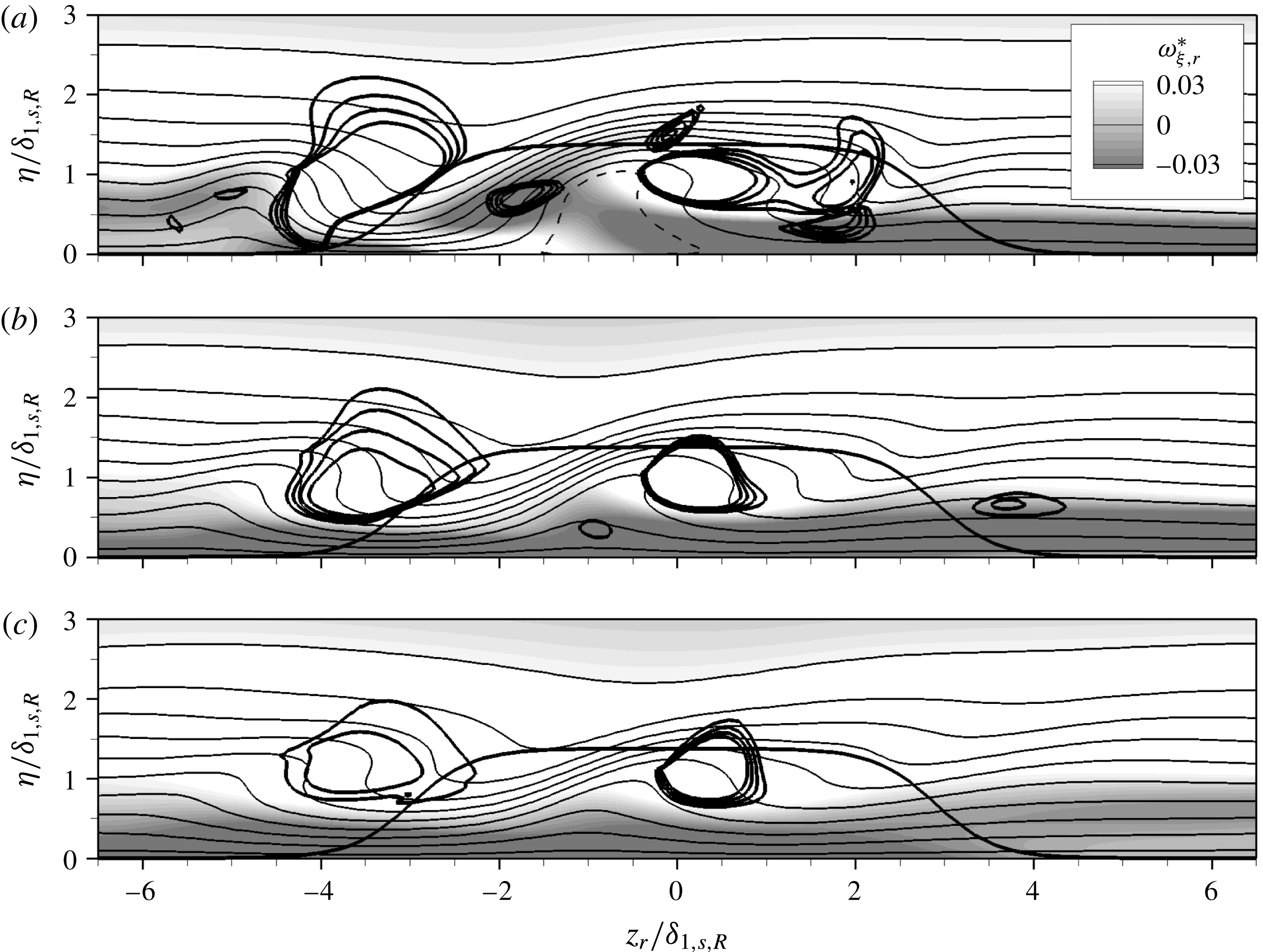
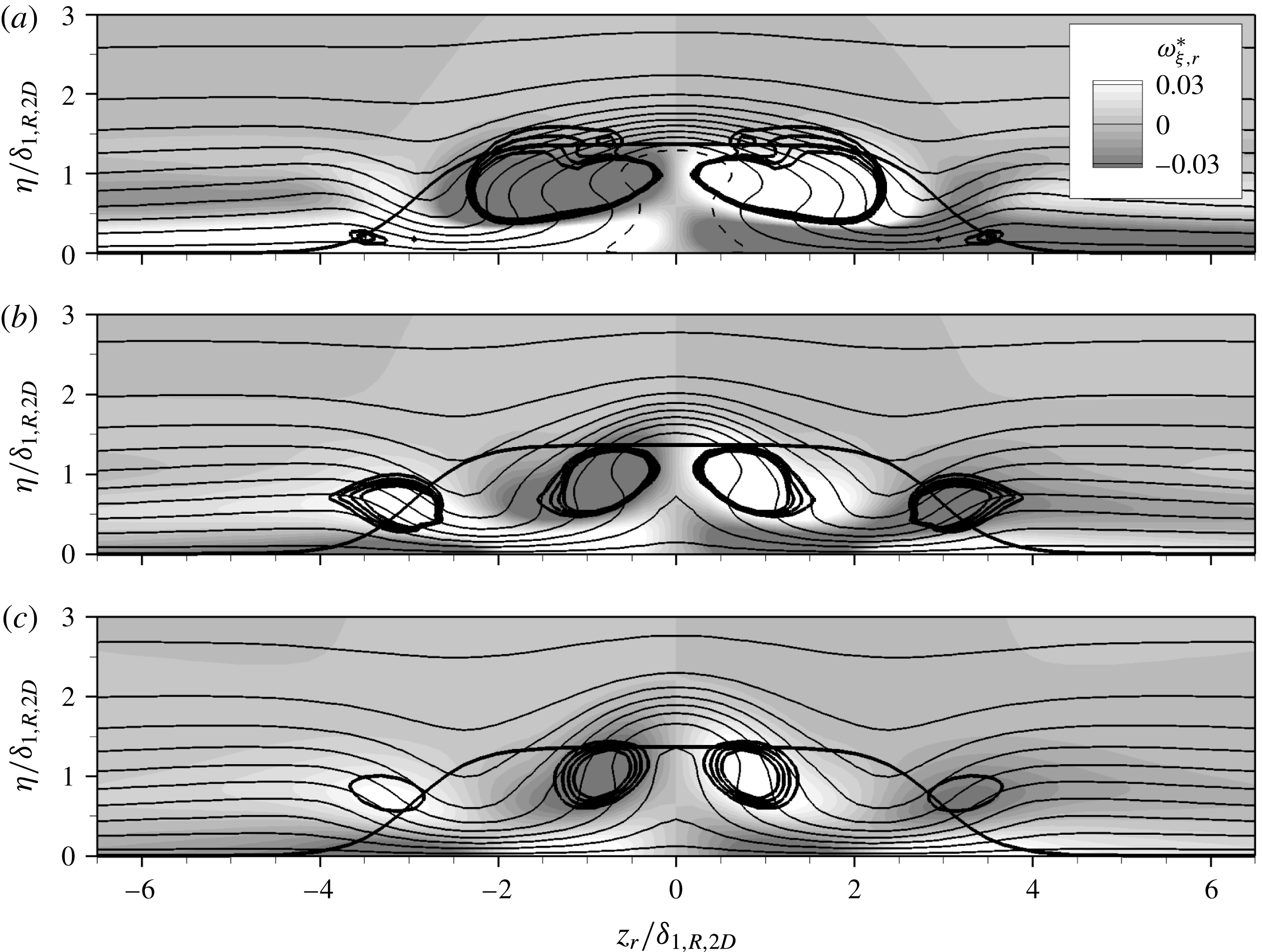
Contours of the downstream velocity component in the rotated system
 $\tilde{u} _{r}$
, normalised by the local edge velocity (tilde denotes normalised values), are given in figure 5(a–c) by the thin solid lines for the three downstream locations
 ${\it\xi}_{r}/{\it\delta}_{1,R,2D}=10.0$
,
 $20.0$
and
 $30.0$
. The positions of the vortex structures are marked by isocontours of
 ${\it\lambda}_{2}^{\ast }$
(thick solid lines), together with the downstream vorticity component
 ${\it\omega}_{{\it\xi},r}^{\ast }$
depicted by the shading. The flow field is symmetric and the rotation sense of the streamwise vortices is clearly illustrated by
 ${\it\omega}_{{\it\xi},r}^{\ast }$
. Around the downstream centreline, a distinct low-speed streak is created by the inner vortex pair through the lift-up of low-momentum fluid away from the wall, as is best seen in figure 5(b,c). The same mechanism gives rise to somewhat weaker low-speed streaks in the outer lateral regions due to the horseshoe-vortex legs.
Two-dimensional case with
 $k=1.365$
,
 $Re_{kk}=487$
: contours of
 $\tilde{u} _{r}$
(solid lines, 0.05–0.95, with increment 0.1; dashed line:
 $\tilde{u} _{r}=0$
) in cross-cuts at (a)
 ${\it\xi}_{r}/{\it\delta}_{1,R,2D}=10.0$
, (b)
 ${\it\xi}_{r}/{\it\delta}_{1,R,2D}=20.0$
and (c)
 ${\it\xi}_{r}/{\it\delta}_{1,R,2D}=30.0$
. The shading depicts the downstream vorticity component
 ${\it\omega}_{{\it\xi},r}^{\ast }$
. Isocontours of
 ${\it\lambda}_{2}^{\ast }$
for
 $-5.0\times 10^{-4}$
to
 $-2.0\times 10^{-4}$
, with increment
 $10^{-4}$
, are indicated by thick solid lines, as is the roughness contour.
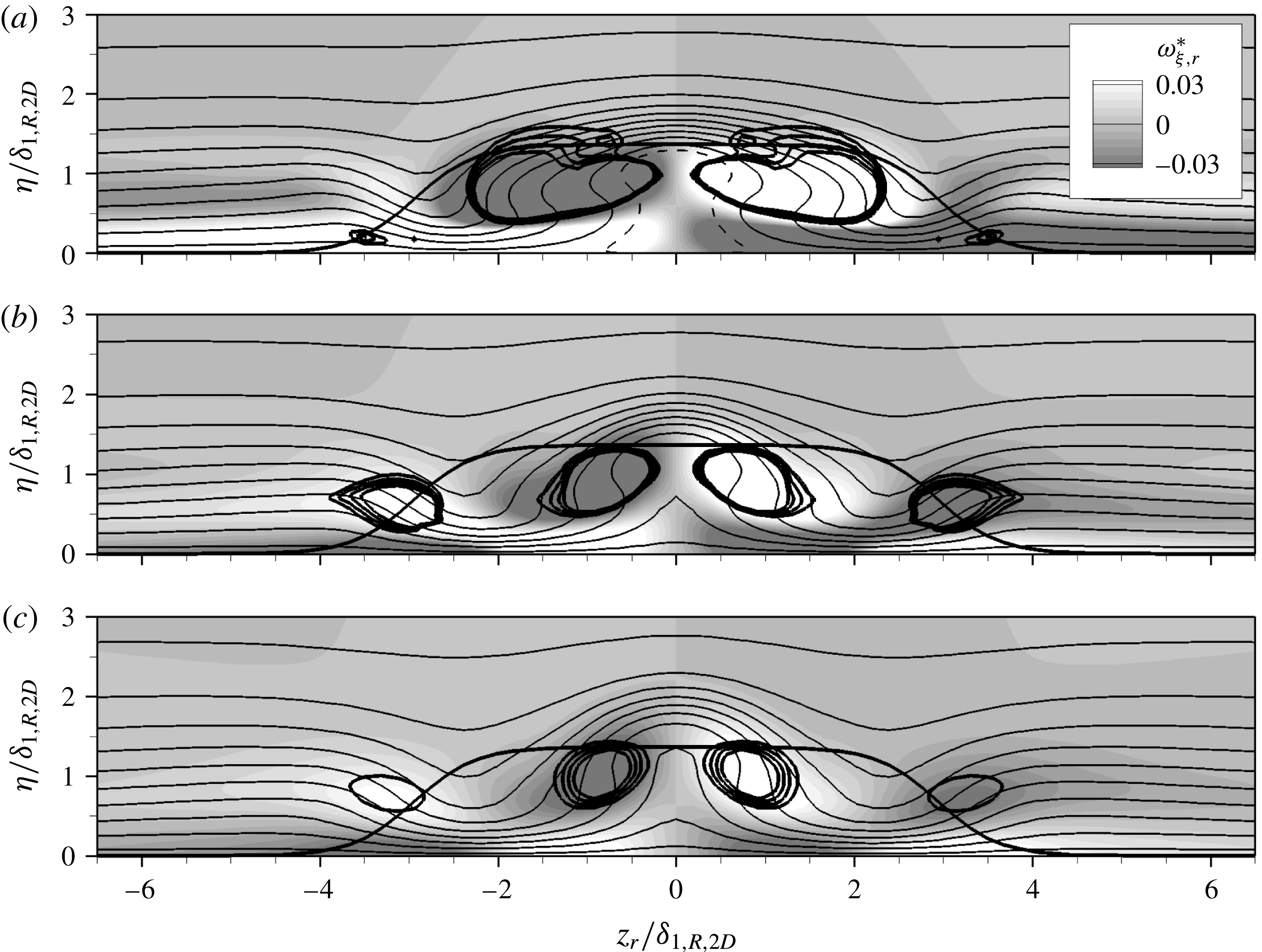
Three-dimensional case with
 $k=1.375,Re_{kk}=487$
: contours of
 $\tilde{u} _{r}$
(solid lines, 0.05–0.95, with increment 0.1; dashed line:
 $\tilde{u} _{r}=0$
) in cross-cuts at (a)
 ${\it\xi}_{r}/{\it\delta}_{1,s,R}=10.0$
, (b)
 ${\it\xi}_{r}/{\it\delta}_{1,s,R}=20.0$
and (c)
 ${\it\xi}_{r}/{\it\delta}_{1,s,R}=30.0$
. The shading depicts the downstream vorticity component
 ${\it\omega}_{{\it\xi},r}^{\ast }$
. Isocontours of
 ${\it\lambda}_{2}^{\ast }$
for
 $-5.0\times 10^{-4}$
to
 $-2.0\times 10^{-4}$
, with increment
 $10^{-4}$
, are indicated by thick solid lines, as is the roughness contour.
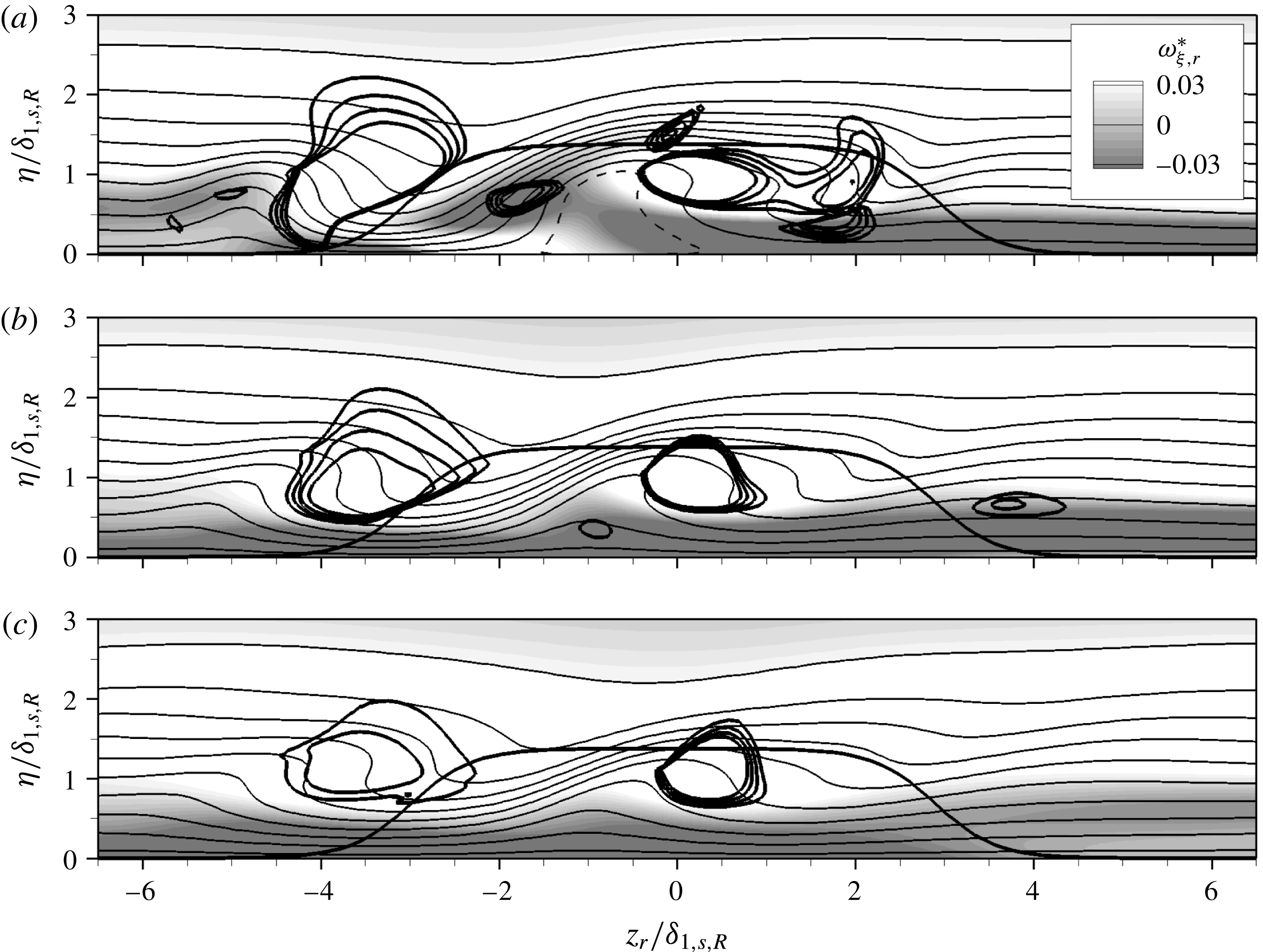
Figure 4(b) illustrates the vortex structures around a roughness element with
 $k=1.375$
,
 $Re_{kk}=487$
in the three-dimensional boundary layer. The flow field becomes asymmetric, but since the coordinate system is aligned with the local flow direction at the boundary-layer edge, some similarities with the two-dimensional case become apparent. Three horseshoe-vortex cores are identified in front of the element; the strongest perseveres. The upper horseshoe leg in figure 4(b) has a sense of rotation conforming to that of a cross-flow vortex, and is supported by the flow. The lower leg has a similar extent as in the two-dimensional case. As in figure 4(a), an inner vortex pair is observed close to the lateral centreline of the roughness. Again, the vortex with a rotation sense conforming to the basic cross-flow direction is supported by the flow, while the other leg is only visible up to
 ${\it\xi}_{r}/{\it\delta}_{1,s,R}=27.0$
.
The contours of
 $\tilde{u} _{r}$
are shown in figure 6(a–c) for the three-dimensional base flow. The downstream vorticity component
 ${\it\omega}_{{\it\xi},r}^{\ast }$
(shading) is dominated by the cross-flow
 $w_{s}$
, which is from right to left in the figure. Only for
 ${\it\xi}_{r}/{\it\delta}_{1,s,R}=10.0$
, figure 6(a), the roughness induces a distinct spanwise modulation of
 ${\it\omega}_{{\it\xi},r}^{\ast }$
. Further downstream, the flow field consists of a layer with negative
 ${\it\omega}_{{\it\xi},r}^{\ast }$
close to the wall and a region of positive
 ${\it\omega}_{{\it\xi},r}^{\ast }$
in the boundary layer above, housing the two dominant vortex legs of the HV and the IV, each being of similar strength in all three cross-cuts. The IV leg with a positive sense of rotation appears stronger than the respective HV leg, indicated by the stronger gradient of
 ${\it\lambda}_{2}^{\ast }$
, i.e. the levels shown are closer. Interestingly, the counter-clockwise rotating IV leg is only visible at
 ${\it\xi}_{r}/{\it\delta}_{1,s,R}=20.0$
, figure 6(b), and is located closer to the wall than its counterpart; further, the velocity contours of
 $\tilde{u} _{r}$
look like a turnover profile created by large-amplitude steady cross-flow vortices. In fact, the left IV leg in the figure seems to be induced on the updraught side of the right leg in a similar fashion to a secondary steady cross-flow vortex, cf. Bonfigli & Kloker (Reference Bonfigli and Kloker2007), and not directly by the roughness.
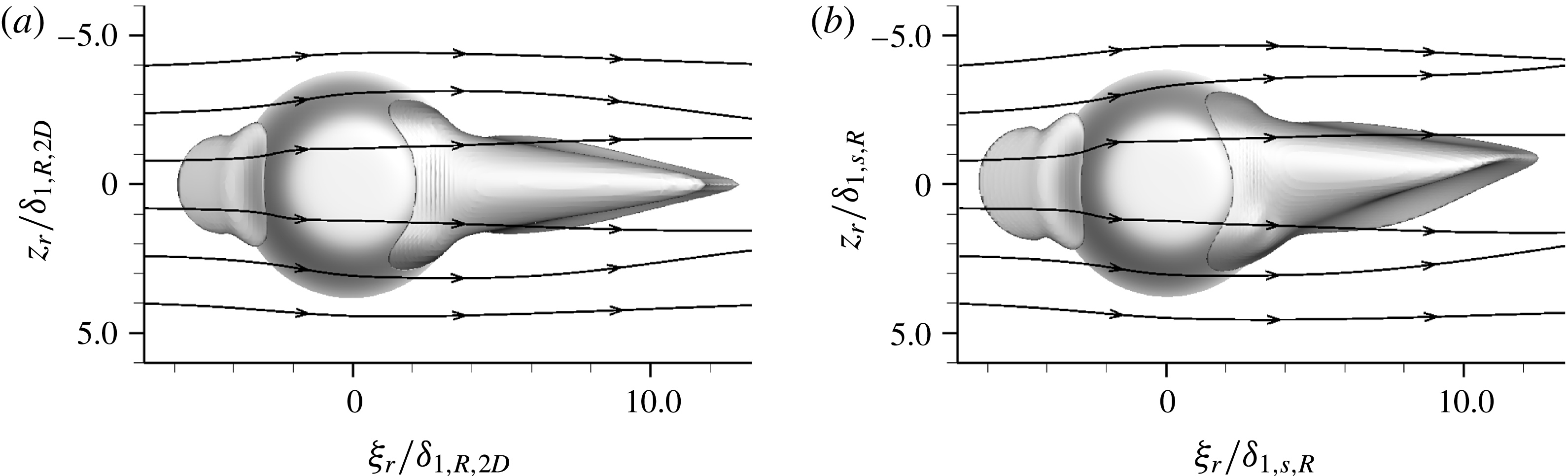
According to the literature, critical-roughness-induced transition is closely linked to unsteady disturbance growth in the recirculation zone behind the elements. Figure 7 compares the regions of negative
 $u_{r}$
for the two- and three-dimensional cases, respectively. In each case, two recirculation regions are observed in front of and behind the roughness, respectively. In the two-dimensional case, figure 7(a), the isosurfaces at
 $u_{r}=-1\times 10^{-4}$
are symmetric with respect to
 $z_{r}=0$
; the aft region is attached to the roughness and extends up to
 ${\it\xi}_{r}/{\it\delta}_{1,R,2D}=12.5$
. With the three-dimensional base flow, figure 7(b), the reversed-flow region in front of the roughness is again symmetric, but the aft recirculation region shows a weak asymmetry after approximately one roughness diameter downstream of the element. Its downstream end is again located at
 ${\it\xi}_{r}/{\it\delta}_{1,s,R}=12.5$
. Apparently, the lateral flow displacement due to the blockage effect of the roughness is stronger than the cross-flow in the boundary layer (being approximately 8.5 % at this position in the smooth-wall flow), therefore masking the asymmetry in the close vicinity of the element. This is confirmed by the streamlines introduced at the left borders of figure 7(a,b) at
 ${\it\eta}/{\it\delta}_{1(,s),R(,2D)}=1$
. The shape and extent of the recirculation zones are very similar for the two- and three-dimensional cases.
Recirculation zones in front of and behind roughness elements, visualised by isosurfaces at
 $u_{r}=-1\times 10^{-4}$
. (a) Two-dimensional base flow,
 $k=1.365$
,
 $Re_{kk}=487$
, (b) three-dimensional base flow,
 $k=1.375,Re_{kk}=487$
. Streamlines are introduced at
 ${\it\xi}_{r}/{\it\delta}_{1(,s),R(,2D)}=-7$
, at a wall distance
 ${\it\eta}/{\it\delta}_{1(,s),R(,2D)}=1$
.
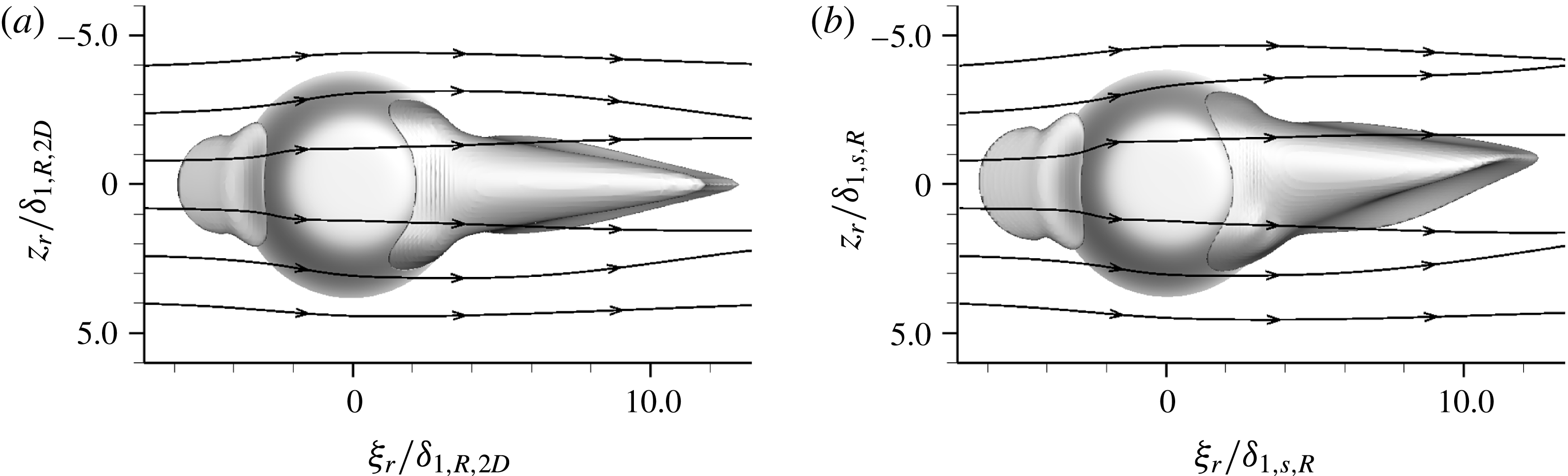
Based on this observation, one may expect similar behaviour of the flow around roughness elements in two- and three-dimensional boundary layers with respect to unsteady disturbance growth in the recirculation zone – but not necessarily in the far wake.
5 Flow tripping
We now concentrate on the effects of discrete roughness elements in the three-dimensional boundary layer. Two transition scenarios can be observed, primarily dictated by the value of the roughness Reynolds number
 $Re_{kk}$
: (i) the leg of the horseshoe vortex corresponding to the basic cross-flow vortex rotation sense is amplified to a high-amplitude cross-flow vortex. Convective secondary instability sets in further downstream, rapidly leading to turbulent flow; (ii) the inherent instability in the recirculation zone behind the element amplifies background disturbances to highly nonlinear amplitudes that persevere and contaminate the flow. Depending on the roughness height, the latter scenario is caused either by strong convective instability of the recirculation zone or absolute instability in the region around the element. Elements that trigger turbulent flow in close vicinity of the element are referred to as near-critical, quasi-critical or (over-)critical roughness elements as will be elucidated hereafter; the roughness Reynolds number
 $Re_{kk,crit}$
constitutes the border between quasi-critical and critical.
Indeed, the decision of which scenario governs the downstream flow is also a matter of the background disturbance level. Computations for elements with
 $k=1.375,Re_{kk}=487$
, where the instability in the aft recirculation zone is still of convective nature, highlight this dependency by the introduction of controlled pulse-like disturbances. We now employ the disturbance strip with two different amplitudes, cf. § 3.4. The simulation results are evaluated by
 ${\it\lambda}_{2}$
-visualisations in the rotated coordinate system showing three fundamental spanwise wavelengths, and by Fourier expansions in time, with frequencies (
 $h={\it\omega}/{\it\omega}_{0}$
) and double Fourier expansions in time and spanwise direction, characterised by the tuple
 $(h,j)$
, where
 $j={\it\gamma}/{\it\gamma}_{0}$
. We perform the Fourier decompositions on the downstream disturbance velocity component
 $\tilde{u} _{s}^{\prime }$
in the edge streamline coordinate system, normalised by the local edge velocity and extract the maximum in
 ${\it\eta}$
–
 $z$
-planes.
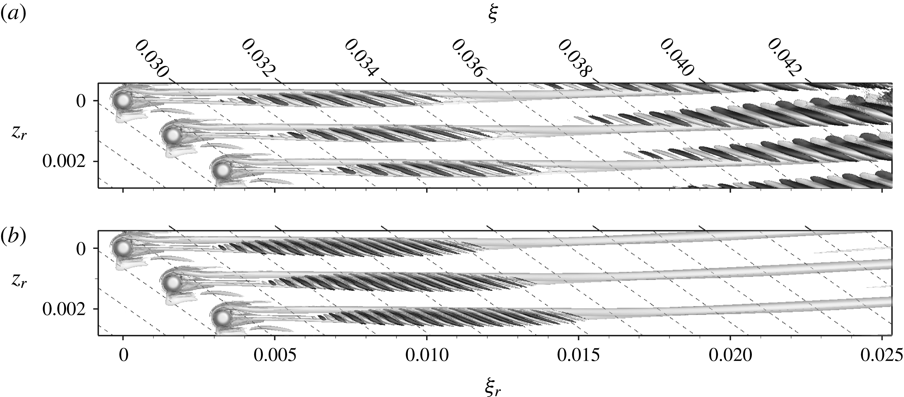
Figure 8(a) shows a snapshot of the wake of the element with
 $k=1.375,Re_{kk}=487$
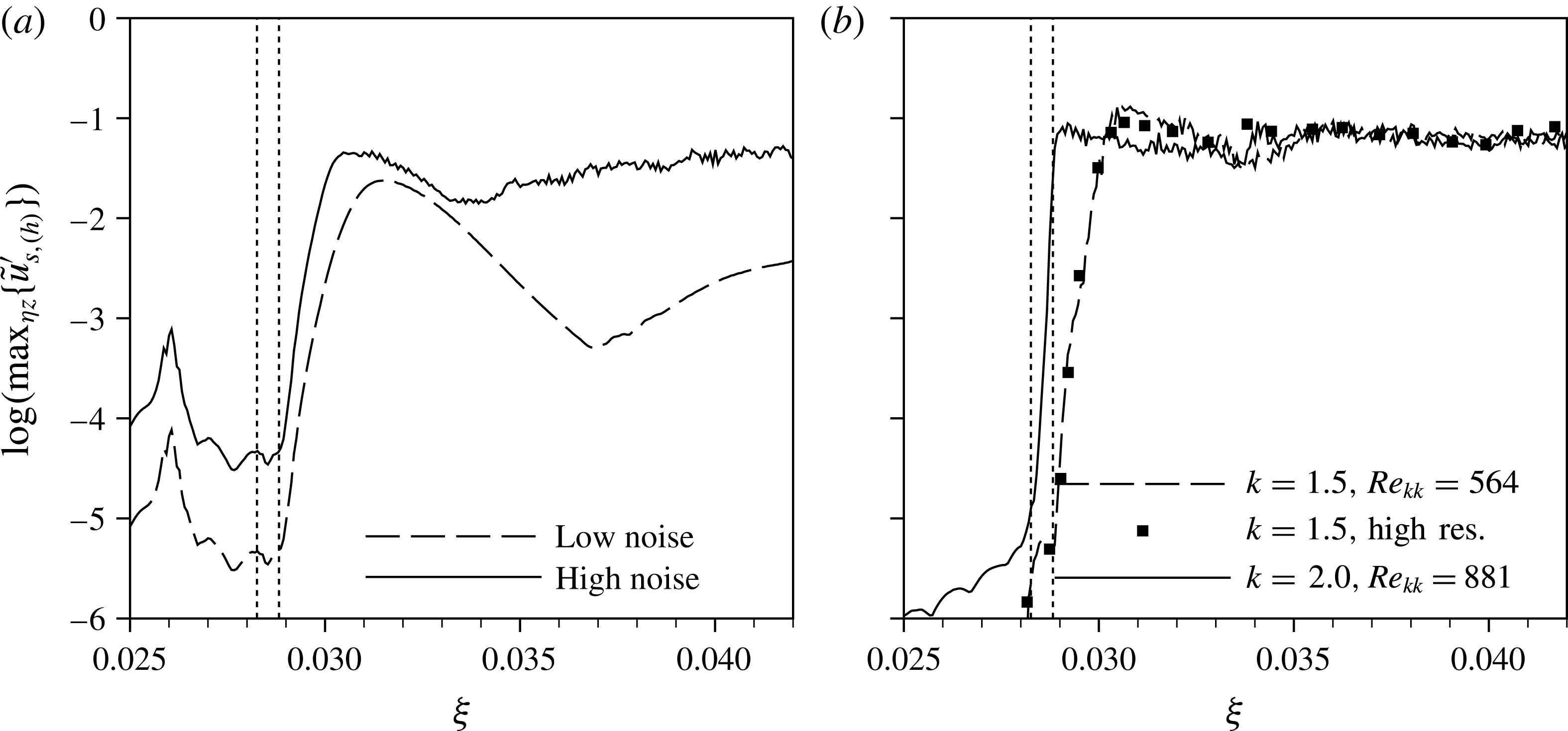
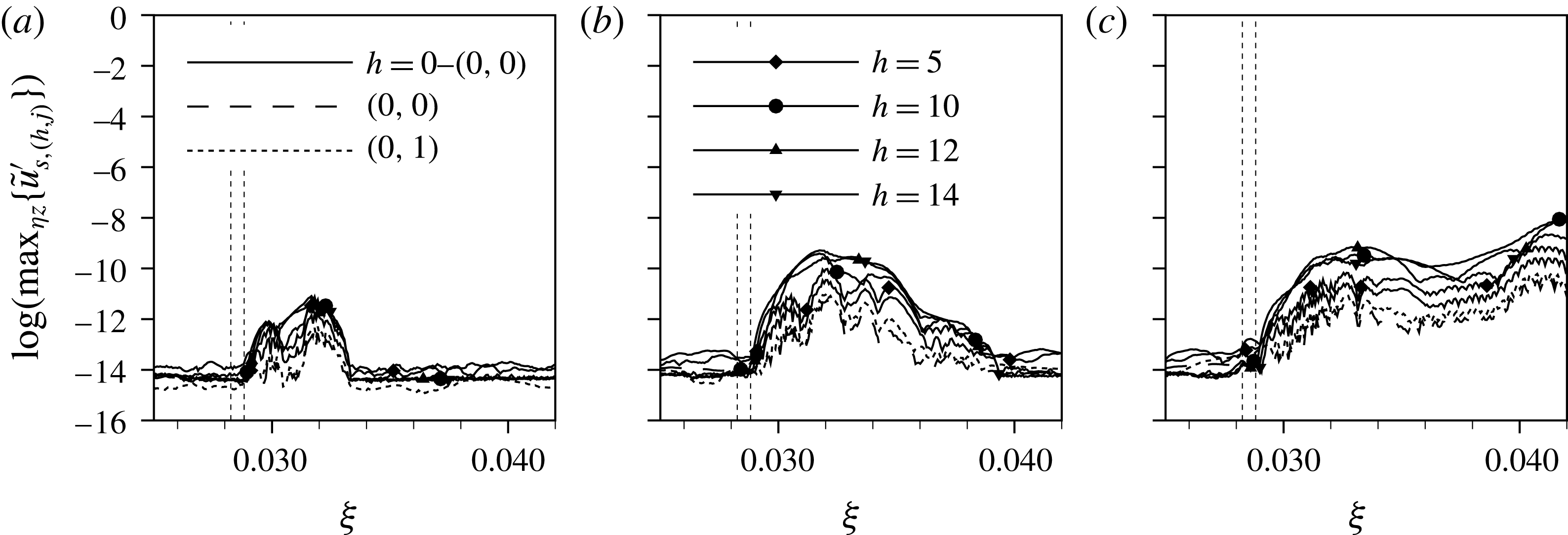
for the low-noise disturbance strip. The periodic quasi-Dirac pulse gives rise to periodically appearing wave packets, being convected downstream. These coherent vortex structures undergo a growth in a confined area behind the elements, and then decay again. This observation is further backed by the Fourier amplitudes of the temporal harmonic
 $h=14$
(cf. figure 9(a), dashed line), showing a strong convective growth right behind the element up to
 ${\it\xi}=0.0315$
. The subsequent decay eventually undergoes a changeover to secondary instability of the cross-flow vortices at
 ${\it\xi}=0.037$
. This is manifested in the
 ${\it\lambda}_{2}$
-visualisation by a weak modulation of the primary cross-flow vortices.
Snapshots of flow past the roughness elements in the rotated coordinate system: (a)
 $k=1.375,Re_{kk}=487$
, low noise, (b)
 $k=1.375,Re_{kk}=487$
, high noise, (c)
 $k=1.5,Re_{kk}=564$
, no controlled disturbance input, (d)
 $k=1.5,Re_{kk}=564$
, no controlled disturbance input, high resolution, (e)
 $k=2.0,Re_{kk}=881$
, no controlled disturbance input. Isosurfaces at
 ${\it\lambda}_{2}=-2.0\times 10^{4}$
, structures above roughness elements are blanked. The black (negative) and white (positive) shading indicates the sign of the streamwise vorticity component
 ${\it\omega}_{{\it\xi},r}$
.

Temporal amplitudes of frequency
 $h={\it\omega}/{\it\omega}_{0}=14$
for the four cases shown in figure 8. (a)
 $k=1.375,Re_{kk}=487$
, two noise levels, (b) no controlled disturbance input, two roughness heights. The dotted vertical lines indicate the roughness position.

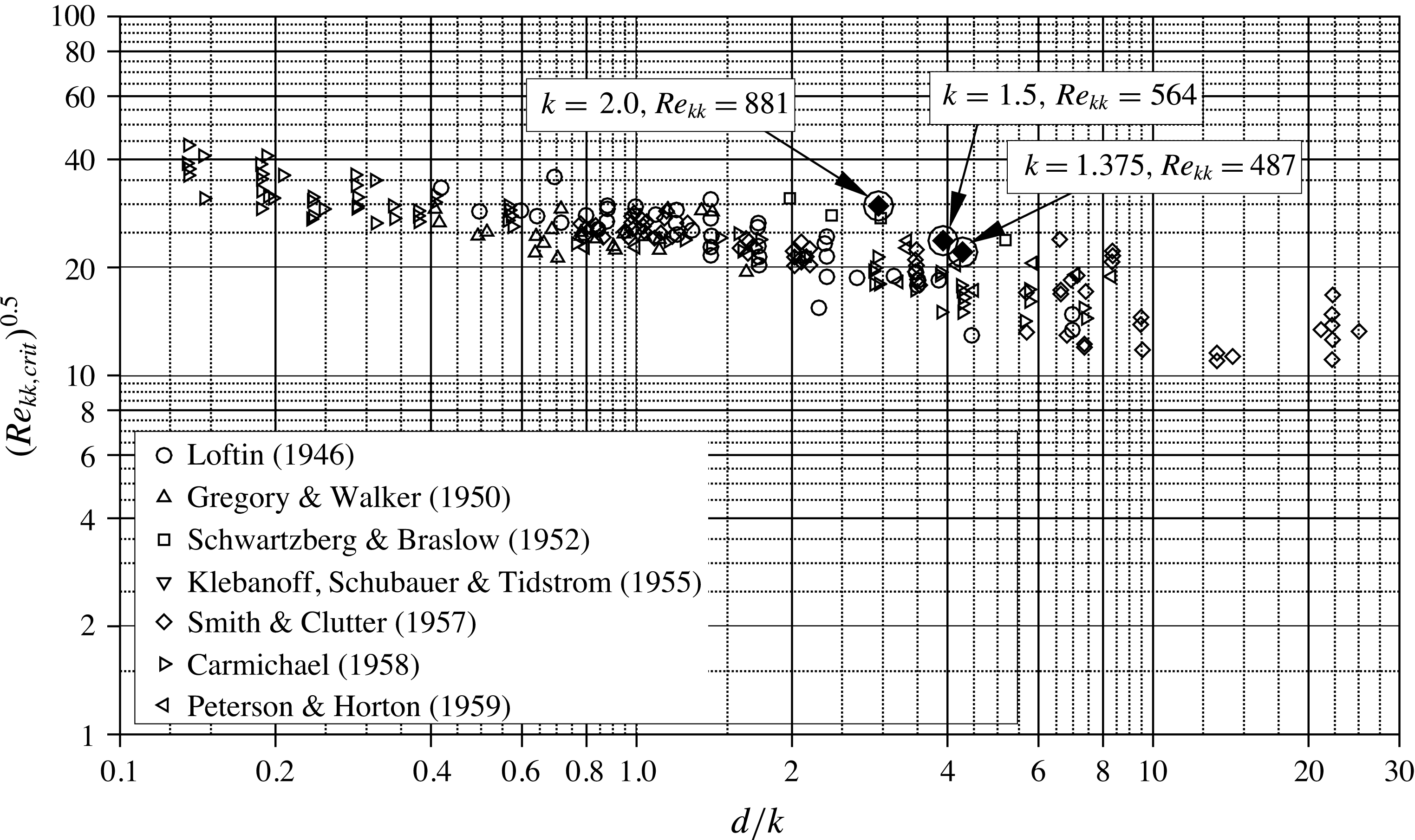
Correlation of the critical roughness Reynolds number
 $Re_{kk,crit}$
in terms of the inverse aspect ratio
 $d/k=1/r_{a}$
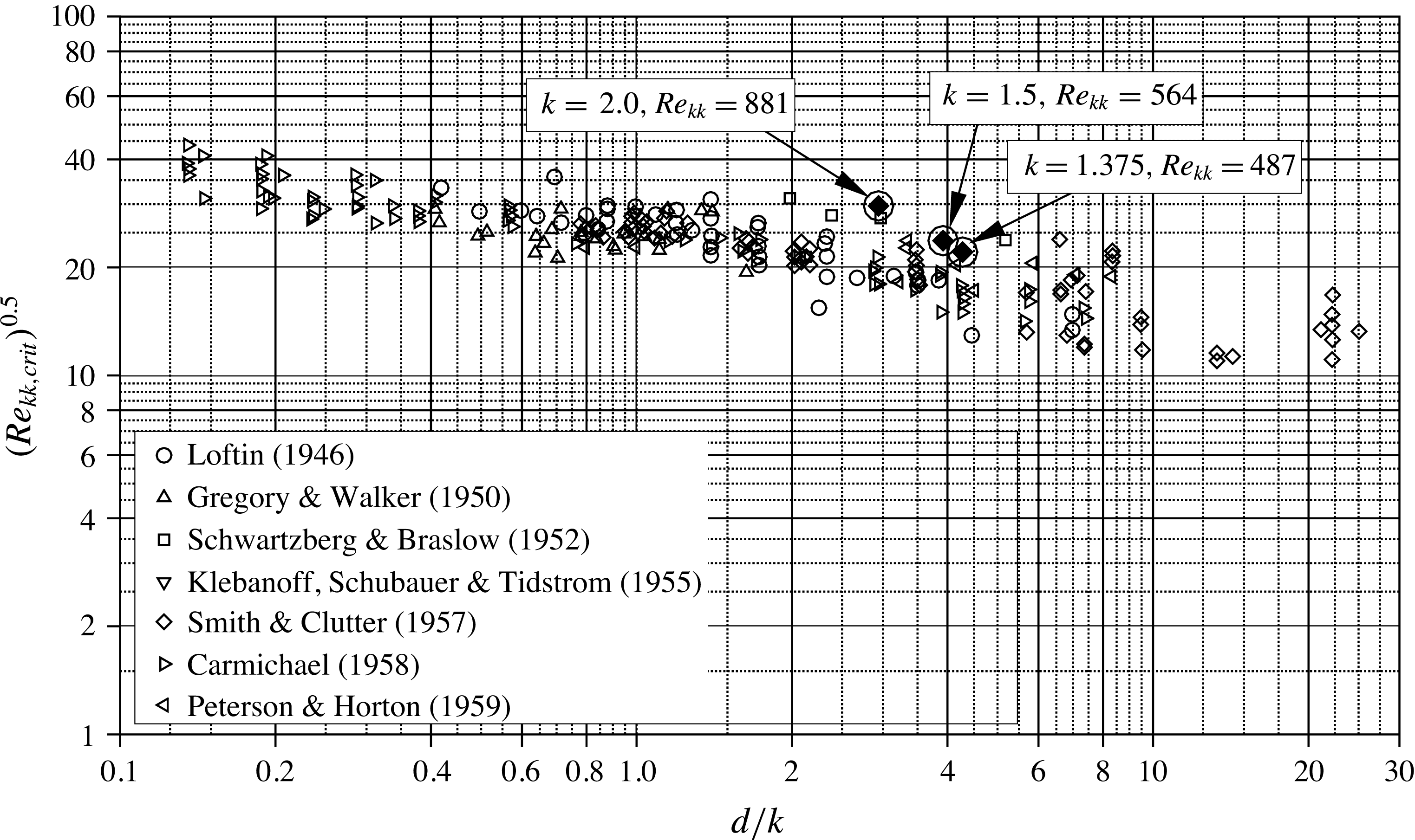
for two-dimensional base flows (reproduction of figure 2 in Von Doenhoff & Braslow (Reference Von Doenhoff and Braslow1961)). The encircled diamonds mark the present results for roughness elements in a three-dimensional base flow.
Temporal Fourier amplitudes for the high-noise set-up, marked by the solid line in figure 9(a), show similar growth rates up to
 ${\it\xi}=0.030$
, but then undergo a nonlinear saturation. Figure 8(b) shows that the initially parallel vortices in the leftmost wave packet begin to break down to smaller structures. The wave packet between
 ${\it\xi}=0.036$
and
 ${\it\xi}=0.039$
, generated by the previous pulse, has already broken down to small-scale structures. Following the previous definition, this element would be labelled near critical; the gaps between the wave packets reveal that the near wake only acts as an amplifier of the incoming pulses, but not as a wavemaker, i.e. there is no region of absolute instability.
The next roughness under consideration has a height of
 $k=1.5,Re_{kk}=564$
, and the disturbance strip is not active, i.e. the incoming background disturbance level is lower than in the previous cases. The flow field is shown in figure 8(c): Within some ten roughness diameters downstream, the boundary layer is contaminated by unsteady vortex structures and transitions to a turbulent state. A convective growth phase up to
 ${\it\xi}=0.03$
is identified for the dashed line in figure 9(b), before the amplitudes saturate at approximately
 $10^{-1}$
; this element is considered quasi-critical, not fully but largely independent of the disturbance background level.
By increasing the roughness height to
 $k=2.0,Re_{kk}=881$
, the near wake becomes absolutely unstable, and thus the flow globally unstable. Consequently, disturbances behind the roughness are temporally amplified until they reach highly nonlinear amplitudes, leading to turbulent structures emanating directly from the roughness elements, see figure 8(d). Fourier amplitudes in figure 9(b) show a sharp rise of the unsteady disturbances right at the position of the roughness. Note that these results are again obtained without the introduction of a controlled disturbance background; the uncontrolled numerical noise suffices.
Based on the four cases shown, the critical roughness Reynolds number for the smooth roughness elements under consideration can be formally given as
 $Re_{kk,crit}\gtrsim 564$
. For free-flight conditions, the low-noise disturbance background is more adequate than the high-noise case, therefore we conclude
 $Re_{kk,qcrit}\approx 560$
to be useful. In the following section, we show that flow past the roughness with
 $k=1.5,Re_{kk}=564$
, although not being globally unstable, is insensitive to the disturbance level in the oncoming flow for large times if there was once a large enough disturbance. In order to relate our findings to previous findings in two-dimensional boundary layers, figure 10 compares our results to the data collected by Von Doenhoff & Braslow (Reference Von Doenhoff and Braslow1961). The quasi-critical element with
 $k=1.5,Re_{kk}=564$
, lies at the upper bound of the clustered region of the data points. Note that the smoothed roughness shape increases the critical value of the roughness Reynolds number slightly, i.e. the respective values for a sharp cylinder are expected to lie somewhat below our results and therefore well inside the data of Von Doenhoff & Braslow (Reference Von Doenhoff and Braslow1961). Thus, our results show that the three-dimensionality of the boundary layer is not crucial for the value of the (quasi-)critical Reynolds number, but for
 $Re_{kk}<Re_{kk,qcrit}$
, the inherent generation of growing cross-flow vortex modes makes the effect of increasing roughness height much smoother than in the two-dimensional case: transition moves forward more continuously.
6 Changeover from convective to global instability
First, we look at
 $k=1.5,Re_{kk}=564$
. A steady flow field is obtained by SFD, then an unsteady DNS in disturbance formulation is conducted, organised in three phases: In phase 1, the simulation is started without the introduction of controlled disturbances and runs for five fundamental periods; only numerical background noise is present. In phase 2, we switch on the disturbance strip with low amplitude (cf. § 3.4) for four fundamental periods, with a temporal envelope ramping the amplitude up and down, i.e. the peak amplitude is reached three times. For phase 3, the disturbance input is switched off again.
6.1 Element with
 $k=1.5,Re_{kk}=564$
, phase 1: no controlled disturbance input

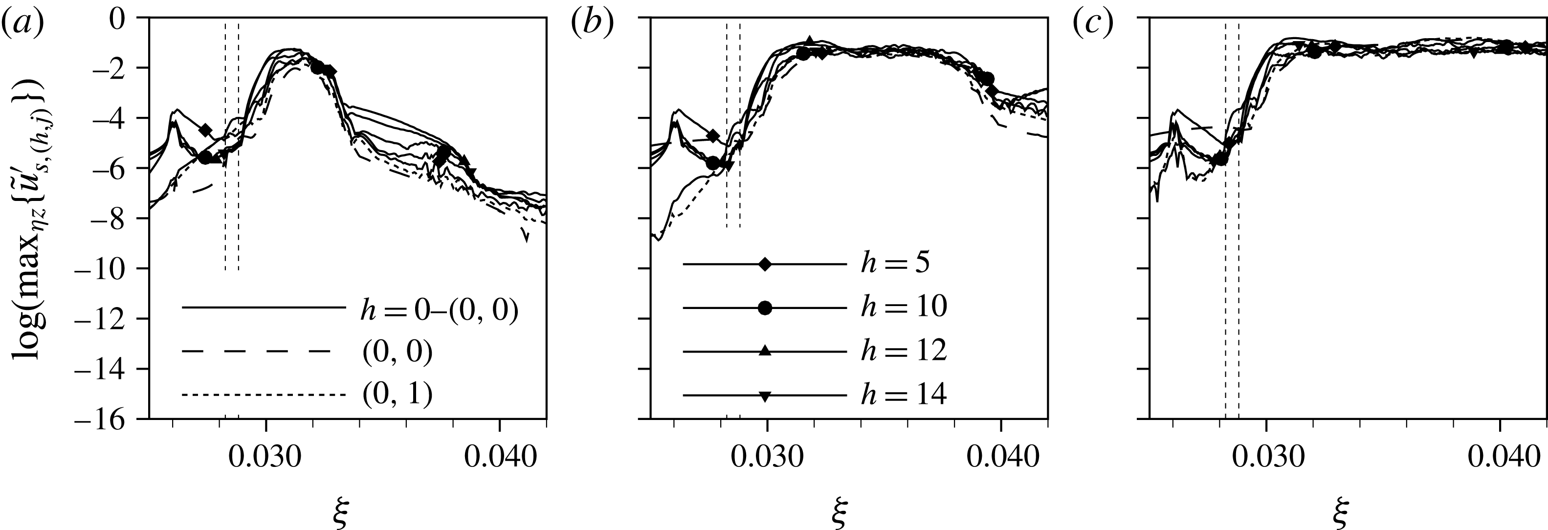
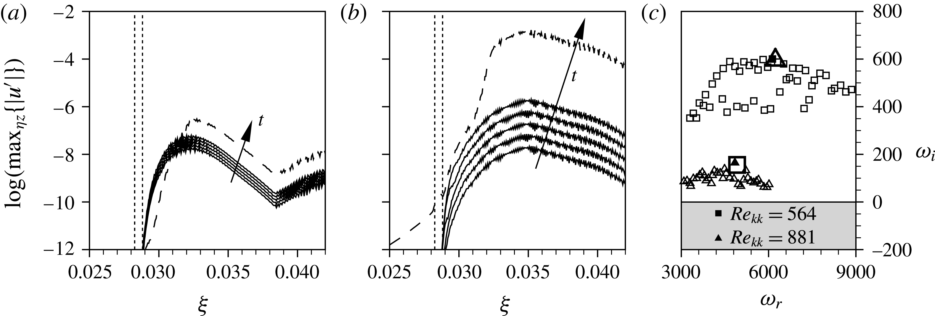
The startup process in phase 1 is illustrated in figures 11 and 12. With increasing time, the background noise is amplified in a region behind the element, and the disturbances undergo a spatial (convective) growth as they travel downstream. Figure 11 shows modal amplitudes of the startup process, each evaluated over one fundamental period. Note that these results are obtained by a Fourier analysis assuming a periodic behaviour in time and therefore constitute a certain averaging of the transient, non-periodic simulation data. The first Fourier plot shows an amplification behind the roughness. In figure 11(b), the dominant modes at
 ${\it\xi}=0.031$
have already reached a time-periodic state after a growth over approximately five orders of magnitude (cf. figure 11
c); a further downstream growth is not yet visible. The Fourier results for periods 4 and 5 are almost identical, figure 11(c) shows data for period 5. No further elevation of the overall disturbance level is expected for longer simulation times, especially since the temporal amplitude evolution shortly behind the roughness has saturated.
Phase 1: modal amplitudes of startup process after SFD for roughness elements with
 $k=1.5,Re_{kk}=564$
, no controlled disturbance input: (a) period 1, (b) period 2, (c) period 5. The dotted vertical lines indicate the roughness position.
Phase 1: vortex visualisations of startup process after SFD for roughness elements in rotated coordinate system with
 $k=1.5,Re_{kk}=564$
, no controlled disturbance input: representative of periods 1–5. Isosurfaces at
 ${\it\lambda}_{2}=-2.0\times 10^{4}$
, structures above roughness elements are blanked. The black (negative) and white (positive) shading indicates the sign of the streamwise vorticity component
 ${\it\omega}_{{\it\xi},r}$
.

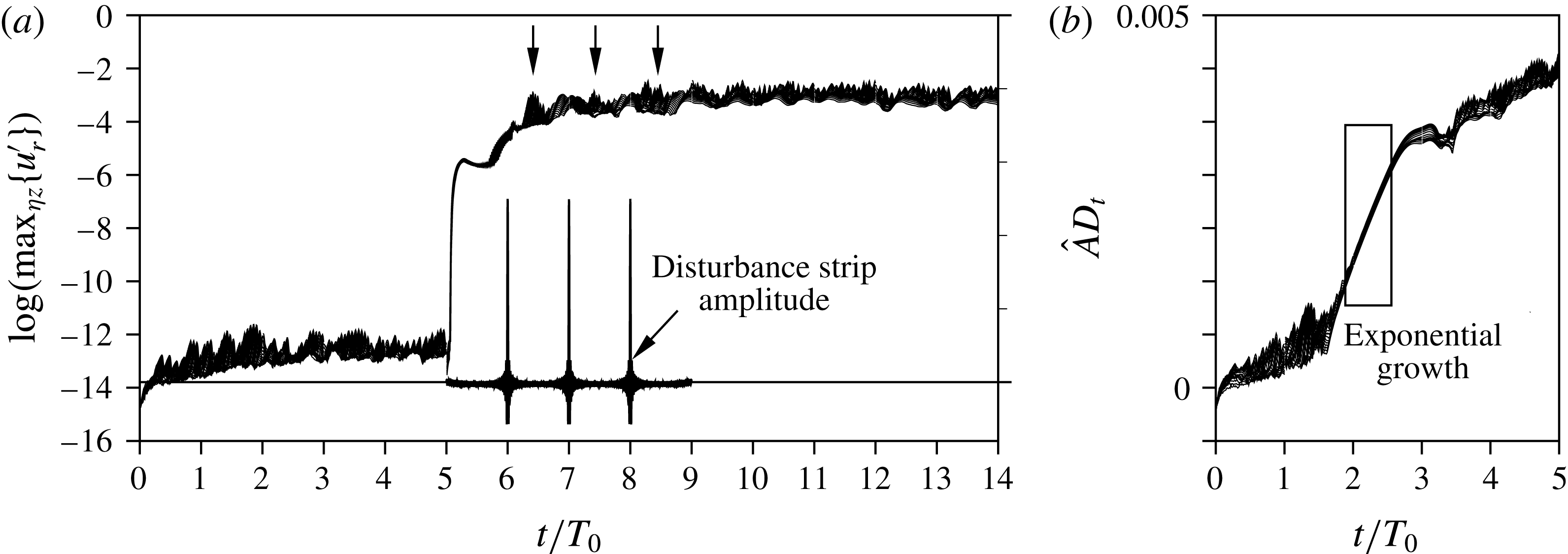
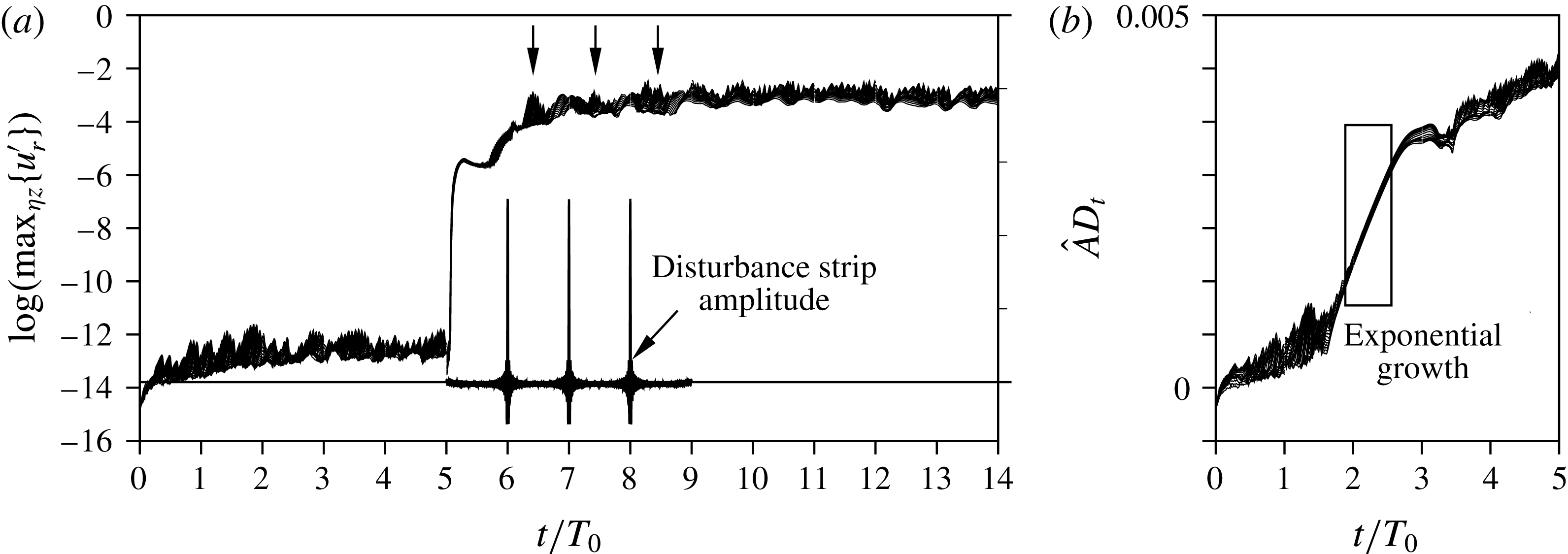
Therefore, all involved instability mechanisms are still of convective nature. Figure 13(a) shows the temporal evolution of in-plane maxima of the disturbance velocity
 $u_{r}^{\prime }$
for several
 ${\it\eta}$
–
 $z_{r}$
-planes in a range of two element diameters behind the roughness; phase 1 is represented by the first five periods. The mean value of all lines settles at approximately
 $10^{-12}$
after
 $t/T_{0}=3$
; no further temporal growth is observed. Evidently, the flow is not globally unstable at these conditions.
Since the disturbance level stays very low, the flow field remains steady from a macroscopic point of view. The vortex visualisation in figure 12 is therefore representative of periods 1–5.
Temporal evolution of in-plane maxima of disturbance velocity
 $u_{r}^{\prime }$
for several
 ${\it\eta}$
–
 $z_{r}$
-planes in a range of two roughness diameters behind the element. Each line corresponds to one
 ${\it\xi}_{r}$
-location. (a)
 $k=1.5,Re_{kk}=564$
, (b)
 $k=2.0,Re_{kk}=881$
.
 $\hat{A}D_{t}$
shows the temporal modulation of the disturbance strip amplitude, the three arrows mark the respective responses in the roughness wake.
6.2 Element with
$k=1.5,Re_{kk}=564$
, phase 2: controlled disturbance input

Phase 2: modal amplitudes of startup process after SFD for roughness elements with
 $k=1.5,Re_{kk}=564$
, with active disturbance input: (a) period 7, (b) period 8, (c) period 9. The dotted vertical lines indicate the roughness position.

We now activate the low-amplitude pulsing upstream of the element, cf. figure 13(a). The disturbance strip is active for four periods. The input raises the overall disturbance level in the computational domain, as can be seen in figure 14(a). Behind the element, the amplitudes are again amplified by four orders of magnitude, up to almost 10 %. Later stages of the startup after the disturbance input is switched on are given in figure 14(b,c) and show how the disturbances saturate at this level and spread over the downstream domain. The relevant stretch for phase 2 in figure 13(a) is
 $5<t/T_{0}<9$
. Shortly after the disturbance source is activated, the amplitudes shoot up sharply. Note that the disturbance strip introduces both acoustic disturbances and vorticity disturbances: the former quickly spread over the domain, see figure 18(a), and raise the associated
 $u^{\prime }$
-disturbance level in the domain to approximately
 $10^{-6}$
, whereas the convectively transported vorticity disturbances are mainly produced by the pulse-like amplitude maxima and therefore come into play only after
 $t/T_{0}=6$
, see the arrows in figure 13(a). The disturbance level raises until the end of phase 2.
The
 ${\it\lambda}_{2}$
-visualisations in figure 15 show how the temporal peaks in the disturbance input initiate quasi-discrete wave packets. In figure 15(a), the first pulse has passed the element, leading to a wave packet at
 ${\it\xi}=0.032$
. In figure 15(b), the centre of the latter has travelled downstream to approximately
 ${\it\xi}=0.037$
and has broken down to a turbulent strip, while the following wave packet at
 ${\it\xi}=0.032$
resembles the one in figure 15(a). The third snapshot, figure 15(c), shows all three wave packets induced by the input pulses. When comparing the wave packets closest to the roughness elements in all snapshots, the one in figure 15(c) seems somewhat more developed than in the two previous figures, although the input from the disturbance strip is the same for all snapshots. Since we found a convective instability behaviour of the flow in § 6.1, this observation can only be explained by either some additional disturbance source or a nonlinearly induced change in the stability characteristics.
6.3 Element with
$k=1.5,Re_{kk}=564$
, phase 3: no controlled disturbance input

Phase 2: vortex visualisations of startup process after SFD for roughness elements in rotated coordinate system with
 $k=1.5,Re_{kk}=564$
, with active disturbance input: last time step of (a) period 7, (b) period 8, (c) period 9. Isosurfaces at
 ${\it\lambda}_{2}=-2.0\times 10^{4}$
, structures above roughness elements are blanked. The black (negative) and white (positive) shading indicates the sign of the streamwise vorticity component
 ${\it\omega}_{{\it\xi},r}$
.

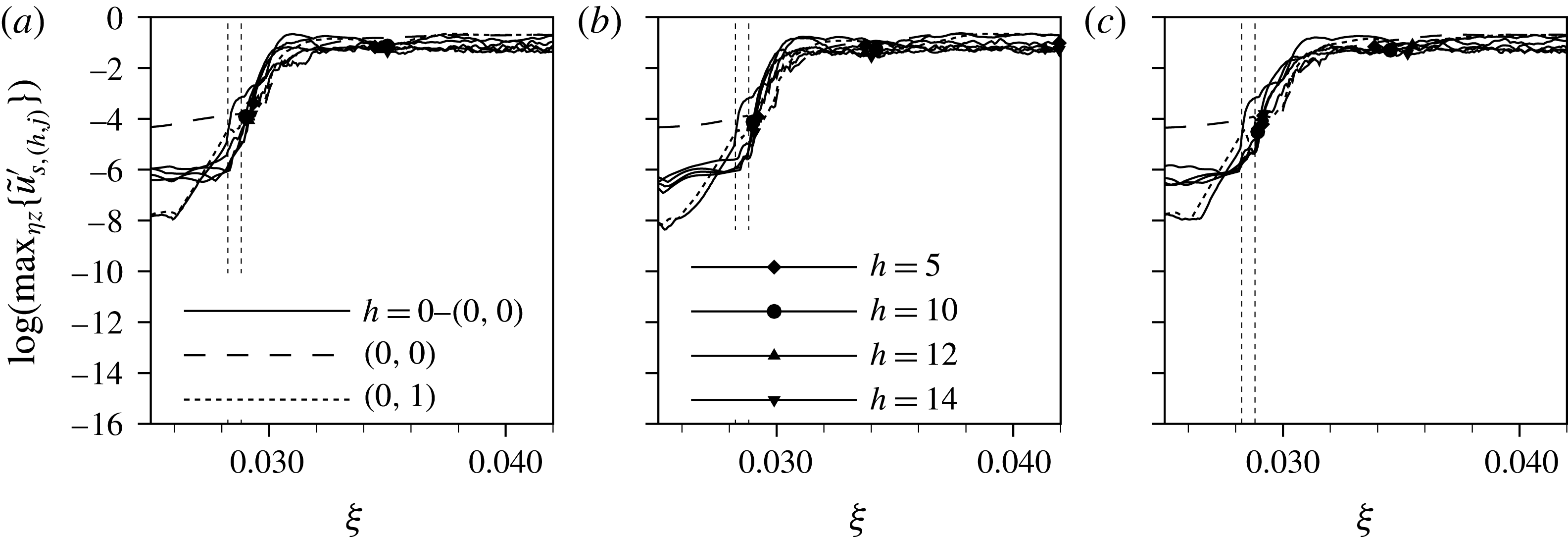
Phase 3: modal amplitudes of startup process after SFD for roughness elements with
 $k=1.5,Re_{kk}=564$
, no controlled disturbance input: (a) period 6, (b) period 8, (c) period 10. The dotted vertical lines indicate the roughness position.
Phase 3: vortex visualisations of startup process after SFD for roughness elements in rotated coordinate system with
 $k=1.5,Re_{kk}=564$
, no controlled disturbance input: last time step of (a) period 6, (b) period 8, (c) period 10. Isosurfaces at
 ${\it\lambda}_{2}=-2.0\times 10^{4}$
, structures above roughness elements are blanked. The black (negative) and white (positive) shading indicates the sign of the streamwise vorticity component
 ${\it\omega}_{{\it\xi},r}$
.

Visualisation of the acoustic field by contours of the disturbance dilatation
 $\text{div}(\boldsymbol{u}^{\prime })$
in a cut at constant
 $z$
through the roughness centre. (a)
 $t/T_{0}=6$
, acoustic signal radiated from the active disturbance strip, with every second wall-parallel grid line starting from index 100 from the wall. (b)
 $t/T_{0}=10$
, noise created by the turbulent boundary-layer structures. The roughness is situated at
 ${\it\xi}=0.285$
. The axes are plotted to scale.

When the controlled disturbance input is switched off, the disturbances behind the roughness elements grow further until the downstream flow field is turbulent after only some 5–10 roughness diameters, see figures 16 and 17. Figure 13(a) shown a constant amplitude level for
 $t/T_{0}>9$
. Although a region of absolute instability could not be found in phase 1, this flow behaves in a globally unstable manner. A possible explanation is a pressure feedback mechanism where the turbulence induced by the temporary disturbance input either changes the base flow in the region of the element and thereby the stability characteristics, or induces strong acoustic noise that travels upstream and is receptive at the roughness. Figure 18(b) depicts the disturbance dilatation at the beginning of phase 3 in a longitudinal cut through the roughness centre. Along the wall, the turbulent boundary layer can be seen, while arched contours outside the boundary layer represent acoustic wave fronts. Clearly, the latter originate from the vortex structures and travel both upstream and downstream, therefore being able to generate new disturbances at the roughness element. Supplementary movie 1, available at http://dx.doi.org/10.1017/jfm.2016.240, shows the time evolution of the structures for all three phases considered in figures 12, 15 and 17.
6.4 Element with
$k=2.0,Re_{kk}=881$
, no controlled disturbance input

As discussed in § 5, the element with
 $k=2.0,Re_{kk}=881$
causes global instability. This can be investigated by a similar approach as before: we employ SFD to obtain a steady flow field and then switch to the disturbance formulation without temporal filtering. The simulation is run over several fundamental periods without the introduction of controlled disturbances, i.e. the disturbance background at the inflow is close to machine accuracy, cf. figure 19(a).
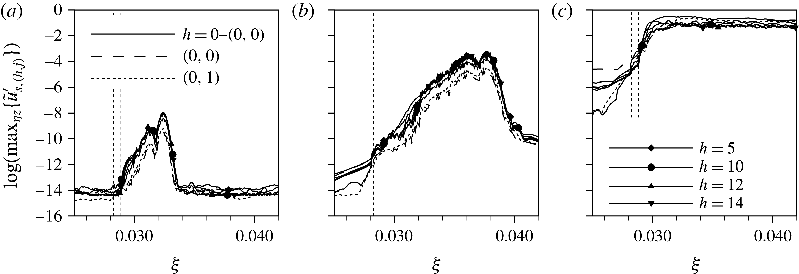
For period 1 (figure 19 a), strong amplification right behind the element is observed. For period 2 (figure 19 b), there is further convective growth downstream but also timewise growth in the roughness region and for period 5 (figure 19 c) the modal amplitudes already indicate turbulent flow downstream of the element.
Figure 20 shows
 ${\it\lambda}_{2}$
-vortex visualisations of the last time step of periods 1, 2 and 5, respectively. Figure 20(a) still shows the steady vortex system obtained by means of SFD. In figure 20(b), finger vortices emerging from the secondary instability mechanism of the steady cross-flow vortices can be observed. The underlying instability mechanism is of convective nature, cf. Wassermann & Kloker (Reference Wassermann and Kloker2002), however, the disturbances are fed by a temporally growing disturbance source (‘wavemaker’) in the recirculation zone right behind the roughness elements. This growing disturbance amplitude continuously shifts the point where the finger vortices can be seen upstream. Eventually, the amplitudes in the region of absolute instability have grown large enough to directly trip turbulent flow, as can be seen in figure 20(c). Note that the shown snapshot does not yet correspond to the fully saturated state, as temporal growth still goes on, see figure 13(b).
Modal amplitudes of startup process after SFD for roughness elements with
 $k=2.0,Re_{kk}=881$
, no controlled disturbance input: (a) period 1, (b) period 2, (c) period 5. The dotted vertical lines indicate the roughness position.
Vortex visualisations of startup process after SFD for roughness elements in rotated coordinate system with
 $k=2.0,Re_{kk}=881$
, no controlled disturbance input: last time step of (a) period 1, (b) period 2, (c) period 5. Isosurfaces at
 ${\it\lambda}_{2}=-2.0\times 10^{4}$
, structures above roughness elements are blanked. The black (negative) and white (positive) shading indicates the sign of the streamwise vorticity component
 ${\it\omega}_{{\it\xi},r}$
.

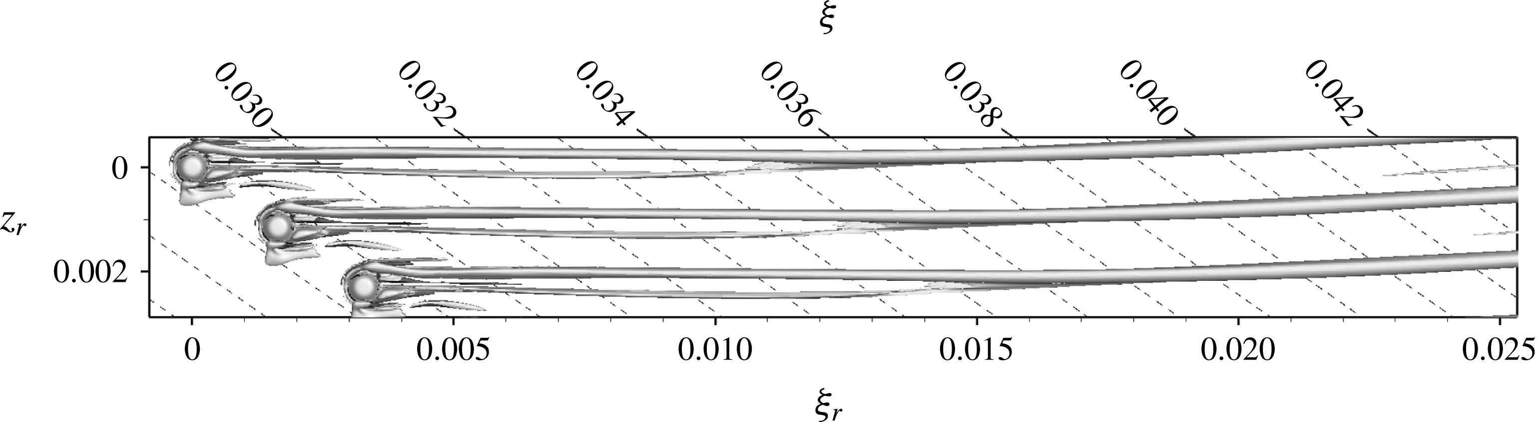
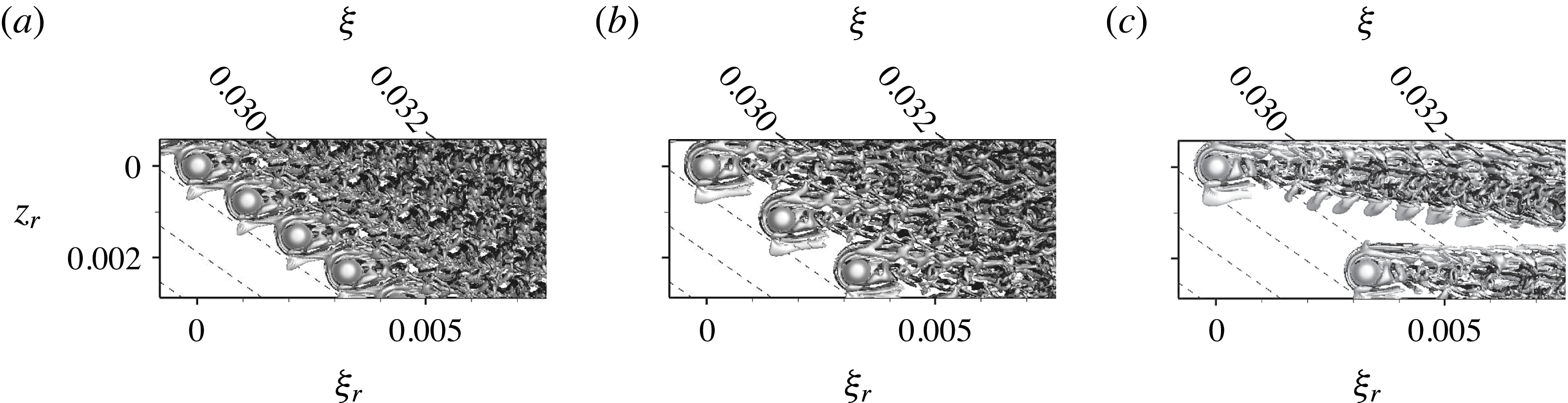
Figure 20(a) shows an interaction of vortices originating from adjacent roughness elements, therefore it may be suspected that the spanwise roughness spacing influences the results. A variation of the spanwise spacing with
 ${\it\lambda}_{z}=2/3{\it\lambda}_{z,0}$
and
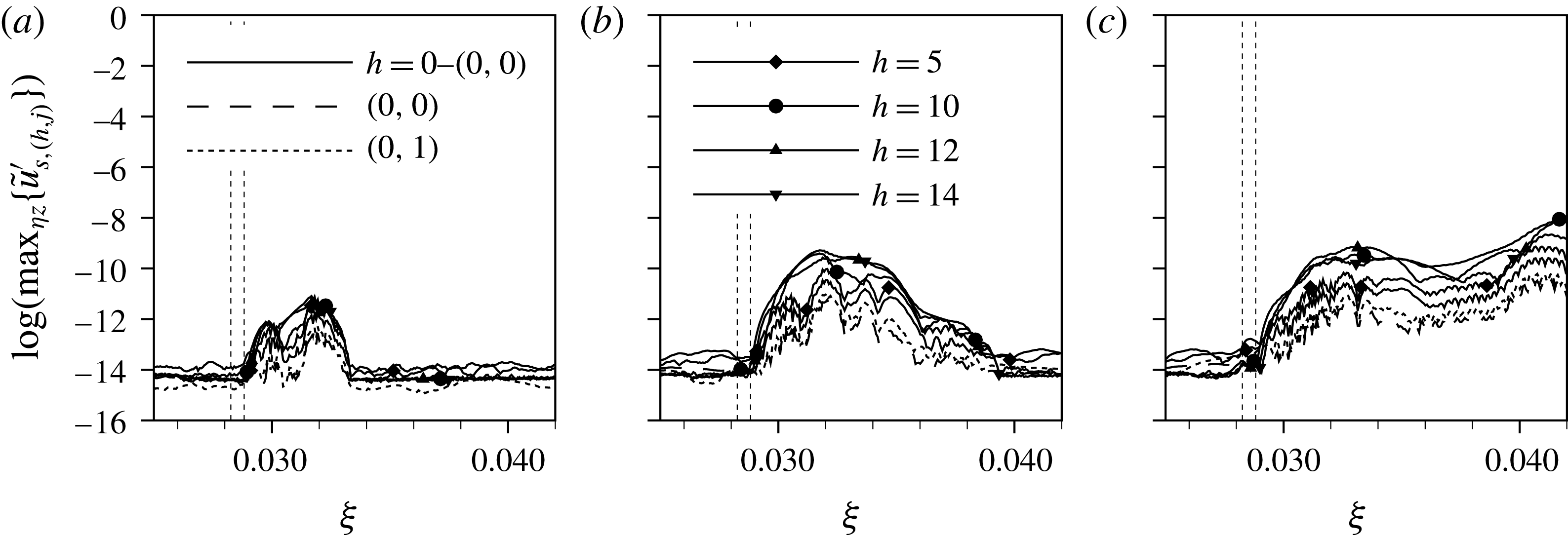
 ${\it\lambda}_{z}=2{\it\lambda}_{z,0}$
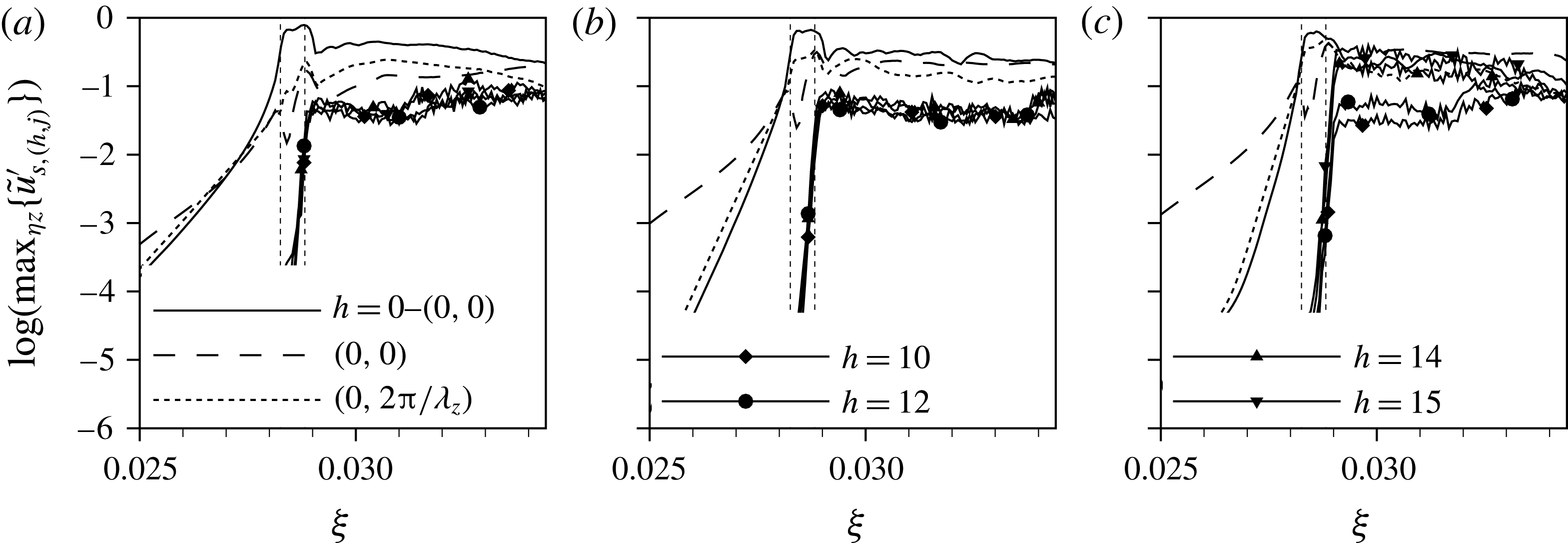
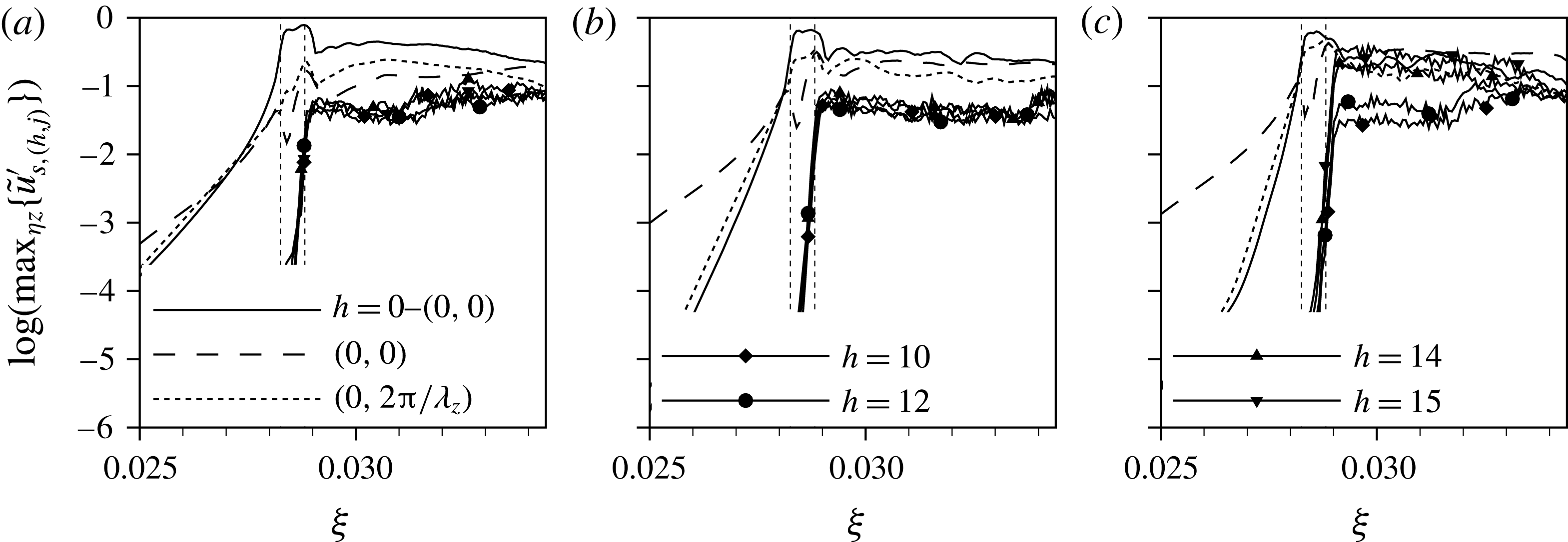
shows only a weak dependence of the flow-tripping quality on the distance between the elements, see figure 21. The Fourier amplitudes in figure 22 show an overshoot of
 $h=14$
and
 $h=15$
behind the roughness for
 ${\it\lambda}_{z}=2{\it\lambda}_{z,0}$
, but the absolute instability in the recirculation zone leads to the same sharp rise of the amplitudes over the roughness elements in all cases. At
 ${\it\xi}=0.034$
, where the complex steady vortex system in figure 20(a) reduces to only one cross-flow vortex per roughness element, the level of unsteady disturbance amplitudes has saturated at the same level for all spanwise spacings.
Snapshots of flow past the roughness elements with
 $k=2.0,Re_{kk}=881$
for different spanwise spacings: (a)
 $2/3{\it\lambda}_{z,0}$
, (b)
 ${\it\lambda}_{z,0}$
, (c)
 $2{\it\lambda}_{z,0}$
, no controlled disturbance input. Isosurfaces at
 ${\it\lambda}_{2}=-2.0\times 10^{4}$
, structures above roughness elements are blanked. The black (negative) and white (positive) shading indicates the sign of the streamwise vorticity component
 ${\it\omega}_{{\it\xi},r}$
.
Modal amplitudes behind roughness elements with
 $k=2.0,Re_{kk}=881$
for different spanwise spacings: (a)
 $2/3{\it\lambda}_{z,0}$
, (b)
 ${\it\lambda}_{z,0}$
, (c)
 $2{\it\lambda}_{z,0}$
, no controlled disturbance input.
The temporal evolution of the in-plane maxima of the disturbance velocity
 $u_{r}^{\prime }$
behind the roughness element is presented in figure 13(b). After a short phase of moderate growth, a distinct region of exponential growth in time can be observed, followed by moderate growth again. (Note that the temporal growth has not saturated yet at
 $t/T_{0}=5$
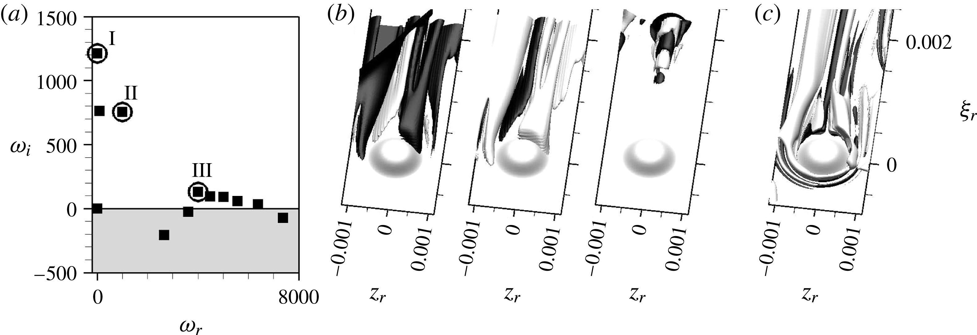
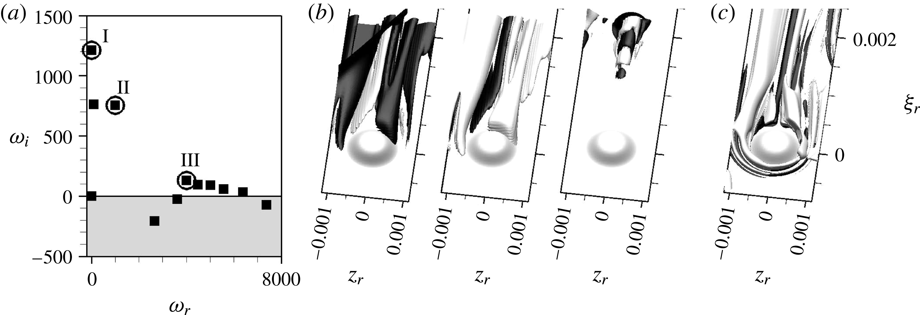
.) The straight lines in the middle region indicate a dominant zero-frequency disturbance in this phase. In order to investigate the root of this behaviour, a dynamic mode decomposition (DMD), see Schmid (Reference Schmid2010), of this confined time frame and
 ${\it\xi}_{r}<0.002$
is performed. The eigenvalue spectrum shown in figure 23(a) contains a set of discrete amplified low-frequency modes and a partially amplified branch at higher frequencies. If the DMD is performed on the time signal before the sharp rise, the discrete low-frequency modes disappear (not shown). The global modes corresponding to the marked modes in the spectrum are given in figure 23(b) by isosurfaces at
 $\pm 10\,\%$
of the maximum downstream velocity disturbance. The shape of modes I and II resembles the steady vortices in figure 23(c). Therefore, these modes are likely to represent a change in strength of the steady vortex system. This in turn may be explained by a modification of the inviscid flow due to an upstream effect of the turbulent boundary layer evolving downstream, explaining the out of line behaviour in the mid region of figure 13(b). The shape of mode III is reminiscent of the unsteady vortices shed from the roughness elements in later stages of the simulation, cf. figure 20(c). Supplementary movie 2 shows the time evolution according to figure 20.
DMD for
 $k=2.0,Re_{kk}=881$
in the confined time frame specified in figure 13(b) and
 ${\it\xi}_{r}<0.002$
. (a) Global spectrum with frequency
 ${\it\omega}_{r}$
and temporal growth rate
 ${\it\omega}_{i}$
, (b) selected global modes, visualised by isosurfaces of the downstream velocity disturbance, i.e.
 $\pm 0.1\max (Re\{\hat{\boldsymbol{u}}_{r}\})$
, (c) isosurfaces show vortices at
 ${\it\lambda}_{2}=-2.0\times 10^{4}$
, the shading indicates the sign of
 ${\it\omega}_{{\it\xi},r}$
, cf., e.g. figure 20.
In conclusion, both roughness elements with
 $Re_{kk}=564$
and
 $Re_{kk}=881$
trigger more or less immediate turbulence, although the above analysis yields real temporal growth only for the larger roughness. For the smaller element, the enhanced noise level in the computational domain due to the downstream appearance of turbulence leads to a self-sustained vortex shedding, once the disturbance level is temporarily increased. This highlights that for large roughness elements in a cross-flow-dominated boundary layer, where the convective growth of a wave packet is not limited to the near wake, the quasi-critical roughness height is not strictly linked to the presence of a global instability, but may be reached before temporal growth in the linear sense, i.e. in three-dimensional global instability analysis, is observed.
7 Global stability analysis
A global stability analysis is performed for the two roughness elements with
 $Re_{kk}=564$
and
 $Re_{kk}=881$
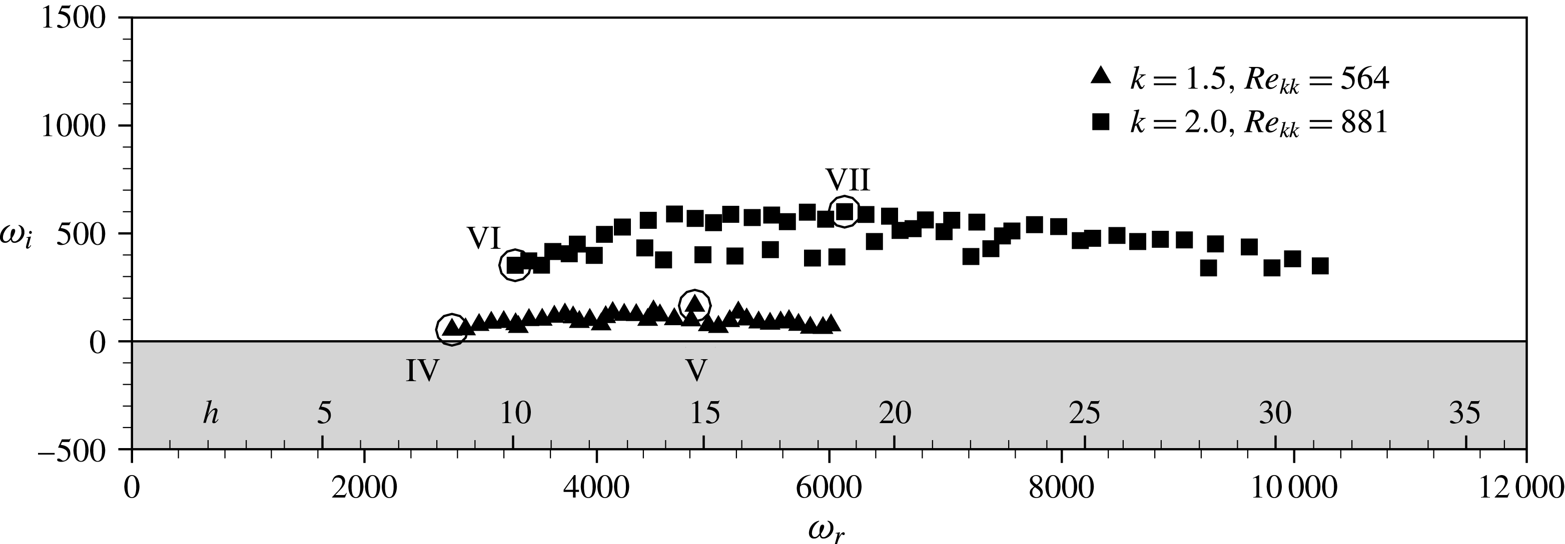
, based on the steady solutions obtained by means of SFD. The global eigenvalue spectra for both cases are given in figure 24. Note that the global stability solver is built upon a verified linearised version of the DNS solver, where, however, the spatial filter for the stretched outflow zone is not yet available with domain decomposition. Instead, we rely on a sponge zone only.
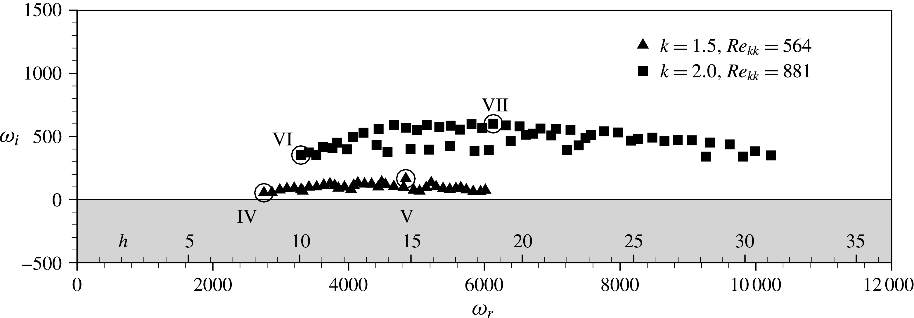
Global eigenvalue spectra for two roughness heights, with frequencies
 ${\it\omega}_{r}$
,
 $h={\it\omega}_{r}/{\it\omega}_{0}$
, and growth rates
 ${\it\omega}_{i}$
. The global modes associated with the encircled symbols are depicted in the figures below.
For
 $k=1.5,Re_{kk}=564$
, the analysis yields a branch of eigenvalues with positive temporal growth rates, with a maximum at
 $h=15$
, matching well the most amplified frequency band in the nonlinear simulations. However, the positive values of
 ${\it\omega}_{i}$
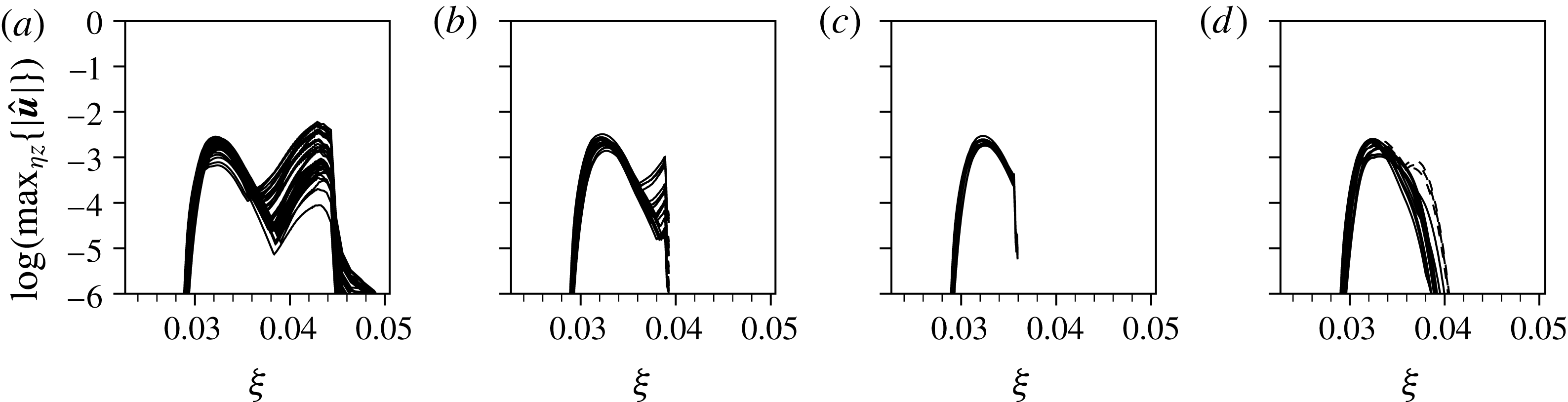
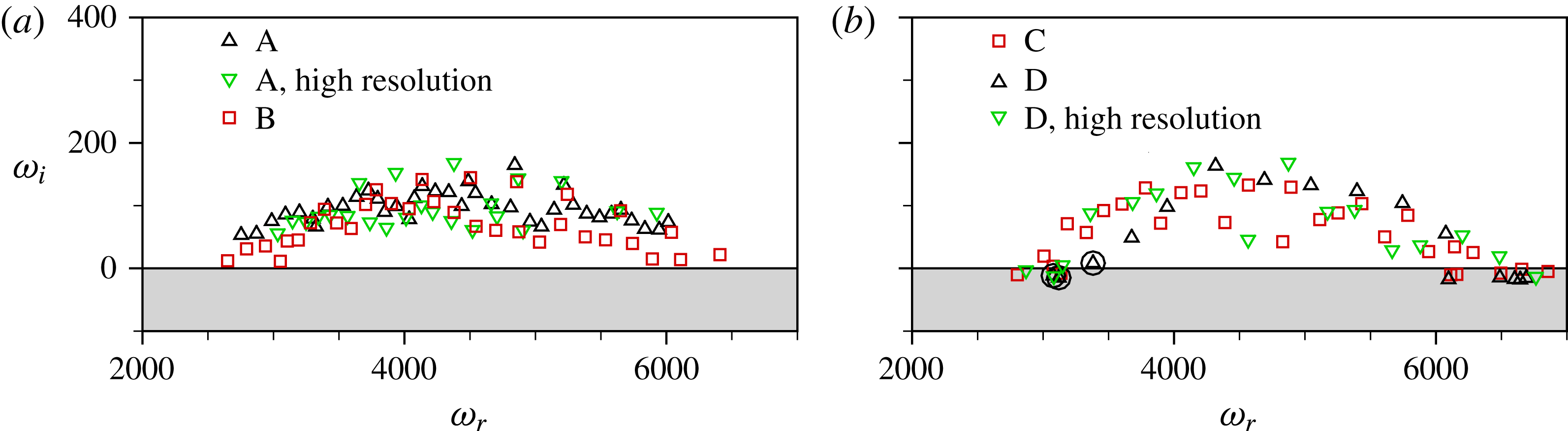
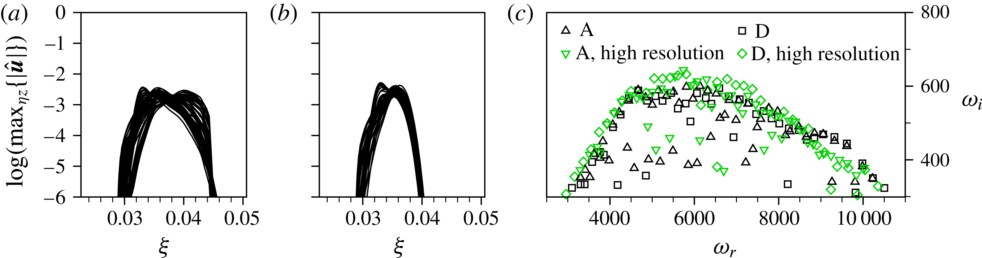
indicate already a global instability, being in contradiction to the findings in § 6.1. Global stability analyses of a roughness wake in a two-dimensional boundary layer by Loiseau et al. (Reference Loiseau, Robinet, Cherubini and Leriche2014) and a jet in cross-flow by Peplinski, Schlatter & Henningson (Reference Peplinski, Schlatter and Henningson2015) show a strong sensitivity of the growth rates to the domain length and the outflow boundary conditions, especially when they are close to neutral stability. Since the observed eigenmodes are localised in the downstream direction in these cases, the authors were able to weaken the sensitivity by using a longer computational domain such that the dominant eigenmodes have decayed considerably before they reach the outflow. In the present flow, however, the secondary instability of the steady cross-flow vortices leads to a convective amplification of unsteady fluctuations, so eigenfunctions do not decay but grow as they approach the outflow, see figure 25(a). Thus, the approach used by Loiseau et al. (Reference Loiseau, Robinet, Cherubini and Leriche2014) and Peplinski et al. (Reference Peplinski, Schlatter and Henningson2015) to mitigate the influence of the outflow boundary does not apply here. As a consequence, we rely on the nonlinear DNS in order to determine whether the flow is globally unstable or not, but use the global modes to give insight in the instability mechanisms and the early linear growth dynamics. A detailed study addressing the sensitivity on the outflow zone treatment is given in appendix A.
Global modes for the roughness case with
 $k=1.5,Re_{kk}=564$
, illustrated by the real part of the rotated complex eigenfunction at
 $\pm 0.05\max _{{\it\Omega}1}(Re\{\hat{\boldsymbol{u}}_{r}\})$
. (a) Mode IV,
 ${\it\omega}=2750+50\text{i}$
, (b) mode V,
 ${\it\omega}=4840+165\text{i}$
. The light grey shading shows the steady vortex system obtained by SFD.
7.1 Global modes for
$k=1.5,Re_{kk}=564$

To illustrate the spatial amplitude distribution and its dependence on frequency, we plot isosurfaces of the real part of the complex, streamwise-velocity eigenfunction in the rotated system, at
 $\pm 0.05\max _{{\it\Omega}1}(Re\{\hat{\boldsymbol{u}}_{r}\})$
where
 ${\it\Omega}_{1}$
denotes the computational domain. The global mode IV in figure 25(a) corresponds to the eigenmode in figure 24 with the lowest frequency, i.e.
 $h=8$
. The mode shows two regions of high amplitude, one in the near wake located on the dominant inner-vortex leg, and one in the far wake on the fully developed cross-flow vortex. As can be seen in the perspective view in figure 26, the two regions are separated by the location where the inner-vortex leg runs into the horseshoe-vortex leg and vanishes. The amplitude distributions
 $|\hat{\boldsymbol{u}}_{r}|$
in the far wake show the familiar shape of a type II mode, see, among others, Balachandar, Streett & Malik (Reference Balachandar, Streett and Malik1992), Koch et al. (Reference Koch, Bertolotti, Stolte and Hein2000) and Bonfigli & Kloker (Reference Bonfigli and Kloker2007), located at the location of maximal wall-normal gradient of the velocity component in the rotated system weighted by the wall distance,
 $y(\partial \tilde{u} _{r}/\partial y)$
. Therefore, the underlying physical mechanism is the secondary instability of cross-flow vortices – an inflectional Kelvin–Helmholtz type instability. Coming back to the near wake, the amplitude distributions show some similarities. Again, the maxima are located on the updraught side of a steady streamwise vortex, but here on the IV leg, in fact being stronger than the HV leg at this downstream location. As the IV decays, the contours of the underlying base flow become less distorted, making the eigenfunction decay as well. In analogy to steady cross-flow vortices, the near-wake instability may therefore be interpreted as a secondary instability of the transiently growing IV leg.
Figure 25(b) shows the global mode V, associated with the most amplified eigenmode at
 $h=15$
. The levels for the isosurfaces are selected as before, but here only the near-wake part of the mode is visible. The far-wake part of the mode is also existent, but does not reach the isosurface level. This indicates that the dominant near-wake instabilities have somewhat higher frequencies than the secondary cross-flow instability.
Global mode IV with
 ${\it\omega}=2750+50\text{i}$
for the roughness case with
 $k=1.5,Re_{kk}=564$
, illustrated by contours of the amplitude part of the rotated complex eigenfunction,
 $|\hat{\boldsymbol{u}}_{r}|$
. Black lines indicate plane contours of the base-flow velocity
 $u_{b,r}$
, the light grey shading shows the steady vortex system obtained by SFD. The
 ${\it\eta}$
-axis is stretched by a factor of 2 for clarity.

Global modes for the roughness case with
 $k=2.0,Re_{kk}=881$
, illustrated by the real part of the complex eigenfunction at
 $\pm 0.05\max _{{\it\Omega}1}(Re\{\hat{\boldsymbol{u}}_{r}\})$
. (a) Mode VI,
 ${\it\omega}=3300+350\text{i}$
, (b) mode VII,
 ${\it\omega}=6130+600\text{i}$
. The light grey shading shows the steady vortex system obtained by SFD.

7.2 Global modes for
$k=2.0,Re_{kk}=881$

For the largest roughness element under consideration, the steady vortex system in the SFD solution shows a qualitative difference to all cases with smaller roughness elements: the streamwise vortices approaching the outflow develop from the IV leg instead of the HV leg. Consequently, the global modes in figure 27 can no longer be separated into a near-wake and a far-wake region, but spread over the downstream extent of the domain without interruption. The global mode VII in figure 27(b) reaches a maximum at
 ${\it\xi}=0.035$
and then starts to decay. This is connected to the transient nature of the underlying streamwise vortex, that has not yet merged with a horseshoe-vortex leg and developed to an ordinary cross-flow vortex. Note that the maximum of the eigenfunction is not in the region of absolute instability/the wavemaker region – but downstream due to the strong convective growth.
8 Conclusions
A detailed DNS study of the effect of cylindrical, finite-size, discrete roughness elements in a three-dimensional boundary layer on a swept wing in the high subsonic flow range has been performed. The diameter-to-height ratio used is approximately 3–4, and the elements are considered in a spanwise row with a spanwise distance corresponding to the most amplified steady cross-flow vortex mode. The main objective was to highlight the physical mechanisms leading to immediate transition due to the presence of the, then critical, roughness, and to compare the results to the well-documented findings for two-dimensional boundary layers.
For subcritical roughness elements, the steady flow fields surrounding the roughness elements in two- and three-dimensional boundary layers show similar features if viewed in the local streamline coordinate system: a set of horseshoe vortices wrapping around the roughness, a large recirculation zone behind the element that is only slightly asymmetric in the three-dimensional case and a set of counter-rotating streamwise inner vortices emerging from the recirculation zone. However, for the three-dimensional case, the vortex structures become asymmetric shortly behind the roughness, where one leg of the inner-vortex system and of one horseshoe vortex are supported by the basic cross-flow. Those vortices merge downstream of the near wake, and lead eventually to one steady cross-flow vortex; transition is initiated by secondary instability of the generated cross-flow vortices in the far wake. We note that in a three-dimensional boundary layer even a far-subcritical roughness is felt downstream due to the generation of exponentially growing cross-flow vortex modes, contrary to two-dimensional flows.
For quasi-critical or critical roughness elements, a purely convective or absolute instability, respectively, in the recirculation zone and near wake leads to unsteady vortex shedding and turbulent flow. The quasi-critical roughness Reynolds number is found to be in the range
 $500<Re_{kk,qcrit}<560$
depending on the background noise and compares well with experimental data obtained in two-dimensional boundary layers at low Mach number. Thus, neither the three-dimensionality of the boundary layer nor a high subsonic Mach number has a dominant effect on
 $Re_{kk,crit}$
if the full velocity vector and the local kinematic viscosity at the roughness height are taken to calculate
 $Re_{kk}$
.
The instability mechanism leading to turbulence tripping evidently is not necessarily a global instability. Rather our nonlinear DNS show that in the quasi-critical range, a purely convective instability behind the roughness may be sufficient to cause (intermittent) turbulence approximately 30–40 displacement thicknesses downstream. Eventually the generated upstream-travelling acoustic waves induce a self-sustaining process if a sufficiently large disturbance passed once. This feedback loop makes the flow field behave like a globally unstable flow.
We also performed a global stability analysis of three-dimensional flow fields made artificially steady. It is based on a matrix-free time-stepper framework using a linearised version of the compressible DNS code. The analysis predicts global instability, albeit weakly, already in the quasi-critical case with
 $Re_{kk}=564$
. The direct, nonlinear DNS shows global instability only for values somewhat higher than that. This result, however, is most likely due to the vulnerability of such instability methods for flow fields close to the first bifurcation, and has also been found by other authors for two-dimensional base flows. (We note again that in our case the outflow treatment in the global solver set-up with a linearised DNS code is currently not as advanced as in the nonlinear DNS code.) In the (quasi-)critical case, the global eigenfunctions show large amplitudes in the medium-wake region of the roughness and further downstream on the steady cross-flow vortices. The former is localized in downstream direction and driven by the locally strong one leg of the inner-vortex system originating in the near wake, while the latter corresponds to secondary cross-flow instability of type II. For larger roughness elements with
 $Re_{kk}=881$
, the scenario is only dominated by the altered behaviour of the stronger inner-vortex leg in the considered computational domain. This leads to eigenfunctions that decay as they approach the outflow boundary of the considered domain.
Acknowledgements
We thank our colleague B. Selent for the support in implementing the global stability solver and for providing the linearised version of the DNS code. This work has been supported by the European Commission through the FP7 project ‘RECEPT’ (grant agreement no ACPO-GA-2010-265094). Computational resources have been provided by the federal high-performance computing center Stuttgart (HLRS) within ‘LAMTUR’.
Supplementary movies
Supplementary movies are available at http://dx.doi.org/10.1017/jfm.2016.240.
Appendix A. Accuracy of the global stability analysis
A.1 Validation with nonlinear DNS code
As a validation of the stability results obtained from the global analysis in § 7, the eigenfunction with the most amplified eigenvalue is added to the temporally stabilised solution. The following startup process in a nonlinear simulation, using the outflow boundary treatment from the linearised stability computations is presented in figure 28(a,b) for the two roughness cases with
 $Re_{kk}=564$
and
 $Re_{kk}=881$
. The lowest envelopes correspond to a time shortly after the beginning of the simulation, the following lines are for increments of
 $0.1T_{0}=0.1(2{\rm\pi}/{\it\omega}_{0})$
. For both roughness elements the envelope shape is kept and the amplitudes increase in time. Thus, the temporal evolution at the beginning of the simulation confirms the existence of temporal modal disturbance growth. The respective growth rates were approximated based on the temporal evolution of the envelope amplitudes at
 ${\it\xi}=0.037$
; the dominant frequencies in the nonlinear simulation were determined by a Fourier analysis. The results shown in figure 28(c) (large hollow symbols) are very close to the eigenvalues of the introduced modes (solid symbols). Overall, the short-time behaviour in the nonlinear simulation with the outflow treatment of the linear simulations is consistent with the global stability results, therefore validating the implementation of the global stability solver and the linearised compressible Navier–Stokes equations.
However, for simulation times longer than
 $0.5T_{0}$
, the temporal growth in the vicinity of the roughness elements is not consistent. For
 $Re_{kk}=564$
, the growth stops and decay sets in, while the envelope shape begins to differ starting from the roughness, see the dashed line in figure 28(a) corresponding to
 $t=T_{0}$
. For
 $Re_{kk}=881$
, figure 28(b), the temporal growth behind the roughness is ongoing, but at a lower growth rate than at the beginning. This ‘transient’ behaviour may be related to the boundary treatment, especially to spurious acoustic reflections at the outflow when spatial filtering is not applied with the streamwise grid stretching; respective investigations are ongoing.
Temporal evolution of the envelope of the most unstable global mode, nonlinear simulation with ‘linear code’ outflow treatment. The interval between the lines is
 $0.1T_{0}$
, the dashed line is at
 $t=T_{0}$
. (a)
 $k=1.5,Re_{kk}=564$
, (b)
 $k=2.0,Re_{kk}=881$
. (c) Hollow symbols: converged spectrum; solid symbols: introduced modes; large hollow symbols: eigenvalues reconstructed from nonlinear simulation.
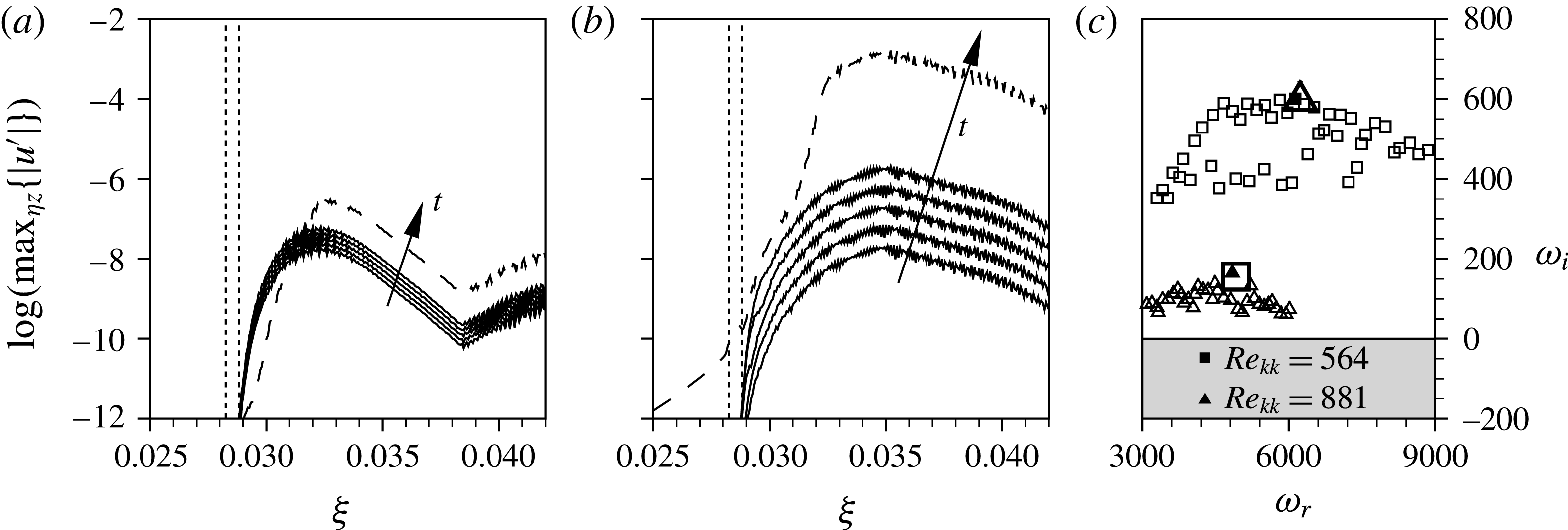
A.2 Sensitivity to the outflow boundary condition and the grid resolution
In order to investigate the sensitivity of our global stability analysis to the outflow boundary condition, the downstream extent of the numerical domain as well as the outflow boundary condition were varied. Figure 29(a) shows the spatial envelope
 $\max _{{\it\eta}z}\{|\hat{\boldsymbol{u}}|\}$
over all converged eigenfunctions for the
 $k=1.5,Re_{kk}=564$
roughness; we show the complete downstream extent of the DNS domain including the stretched outflow zone starting at
 ${\it\xi}=0.0424$
. Up to approximately
 ${\it\xi}=0.036$
, the growth is dominated by the near-wake instability, before a kink in the lines indicates the changeover to the convective secondary instability of the steady cross-flow modes in the SFD solution. The relatively large amplitude in the downstream region is believed to cause the sensitivity to the outflow boundary condition. In an attempt to decrease the amplitude at the outflow, the domain was truncated or the sponge region in front of the outflow boundary was extended in upstream direction, see table 3. The amplitudes for configurations B-D are shown in figure 29(b–d). (The dashed lines in figure 29
d showing a second peak at
 ${\it\xi}=0.038$
correspond to low-frequency modes with small positive or negative temporal growth rates, see the encircled symbols in figure 30
b.) The associated global spectra are shown in figure 30, where the dependence on the numerical set-up is clearly visible. However, the maximum amplification rate as well as the amplified frequency range compare in all cases. The same holds for spectra obtained on the high-resolution grid for configurations A and D.
Configurations used for the sensitivity study, with
 ${\it\xi}_{stretch}$
being the beginning of the stretched outflow zone (if applicable),
 ${\it\xi}_{sponge}$
the location where the volume forcing in front of the outflow boundary sets in and the position of the outflow boundary
 ${\it\xi}_{outflow}$
.
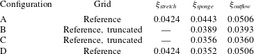
Envelopes of all converged global eigenfunctions for
 $k=1.5,Re_{kk}=564$
, obtained with the different numerical set-ups given in table 3: (a) reference configuration A, (b) truncated configuration B, (c) truncated configuration C, (d) configuration D with extended sponge zone in front of the outflow boundary.

Global eigenvalue spectra for
 $k=1.5,Re_{kk}=564$
, obtained with the different numerical set-ups given in table 3: (a) reference configuration A, truncated configuration B; (b) truncated configuration C, configuration D with extended sponge zone in front of the outflow boundary.
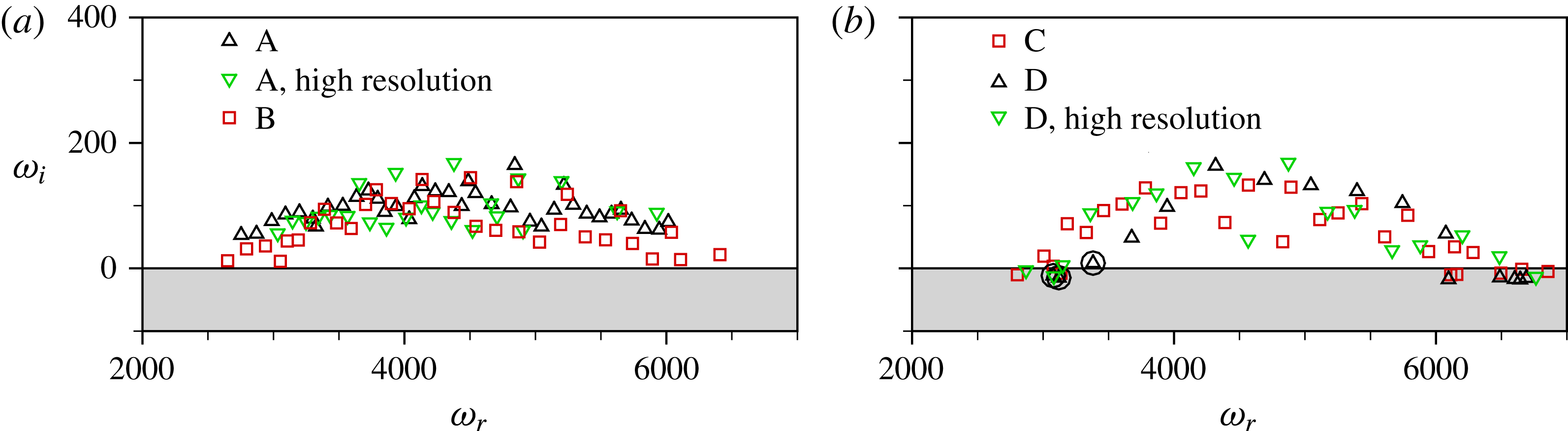
For the roughness with
 $k=2.0,Re_{kk}=881$
, the amplitudes in figure 31(a) may be assigned to three groups, according to the downstream position where the maximum is reached: Eigenfunctions with the highest frequencies reach their maximum at
 ${\it\xi}=0.032$
, followed by a group of highest temporal growth rates having their amplitude peak at
 ${\it\xi}=0.036$
, before the low frequency modes reach their maximum at
 ${\it\xi}=0.040$
. Again, we perform a second global stability analysis with the extended sponge zone on front of the outflow boundary starting at
 ${\it\xi}=0.0353$
; the respective envelopes of the eigenfunctions are given in figure 31(b). Here, the overall sensitivity of the spectra given in figure 31(c) is weaker, however, especially in the most amplified frequency range
 $4250<{\it\omega}_{r}<7000$
, the deviations are largest, which may be connected to the fact that the sponge zone begins close to the point where the connected eigenfunctions reach their spatial maximum. A grid study with the high-resolution grid yields somewhat larger maximum amplification rates. We note that the outflow zone of the high-resolution mesh has the same physical length as the reference grid, but the resolution is not relaxed to the same large step size. Thus, the dissipation effect in the outflow zone is weaker.
Envelopes of all converged global eigenfunctions for
 $k=2.0,Re_{kk}=881$
, obtained with different numerical set-ups given in table 3: (a) reference configuration A, (b) configuration D with extended sponge zone in front of the outflow boundary. (c) Associated global eigenvalue spectra: reference configuration A, configuration D with extended sponge zone in front of the outflow boundary.
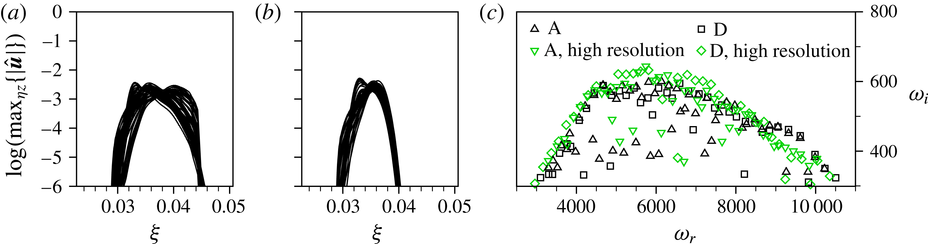
In conclusion, a dependence of the global spectra on the outflow boundary condition and its position is especially evident for the roughness with
 $k=1.5,Re_{kk}=564$
, but stays within an acceptable low tolerance level, corroborating the validity of the basic findings.