1 Introduction
During the last several years there has been an intensive study of basic waves modes and instabilities (Merlino et al. Reference Merlino, Barkan, Thompson and D’Angelo1998; Ostrikov et al. Reference Ostrikov, Yu, Vladimirov and Ishihara1999; Ghosh, Khan & Gupta Reference Ghosh, Khan and Gupta2006b ; Shukla & Stelflo Reference Shukla and Stelflo2007; Rosenberg Reference Rosenberg2009, Reference Rosenberg2013) in dusty plasmas. Today, it is well established that in most of the astrophysical and laboratory plasmas, the dust grains become negatively charged because of the attachment of electrons on the dust grain’s surface (Ostrikov, Kumar & Sugai Reference Ostrikov, Kumar and Sugai2001; Ghosh, Khan & Bharuthram Reference Ghosh, Khan and Bharuthram2006a ; Merlino & Kim Reference Merlino and Kim2006). In most of the weakly ionized laboratory and space plasmas, the ionization of a neutral gas plays a very important role in determining overall characteristics of the plasma (Shukla & Morfill Reference Shukla and Morfill1996). Consequently, the physics of ionization instability (D’Angelo Reference D’Angelo1997, Reference D’Angelo1998) has become a much more interesting topic.
The main reason for this instability is the difference of ionization rates in the wave crest and trough. The regions corresponding to the wave crests have higher potential than that at the troughs. As a result, the electrons at the crest gain energy from the wave potential and are therefore accelerated due to the higher energy. The other electrons are also accelerated by the wave but with different energies corresponding to their position on the wave profile. The accelerated electrons may have attained sufficient energy to ionize a neutral gas atom on collision. As the cross-section of ionization increases rapidly with energy of the incoming electrons, the rate of ionization will be faster at the wave crest than that at the troughs i.e. the plasma density perturbation at the wave crest and trough are not in unison (D’Angelo Reference D’Angelo1997). This increasing difference in ionization rate leads to an instability in the medium known as the ionization instability.
It is well known that the wave mode can be excited in a plasma due to several dissipative mechanism such as ionization, recombination and collisions (Kaw & Singh Reference Kaw and Singh1997; Ivlev et al.
Reference Ivlev, Samsonov, Goree, Morfill and Fortov1999; Nakamura, Bailung & Shukla Reference Nakamura, Bailung and Shukla1999; Avinash Reference Avinash2001; Nakamura & Sharma Reference Nakamura and Sharma2001). Long before, Akhiezer, Akhiezer & Angeleiko (Reference Akhiezer, Akhiezer and Angeleiko1970) and Johnson, D’Angelo & Merlino (Reference Johnson, D’Angelo and Merlino1990) had found that ionization causes instability of ion acoustic waves (IAWs) in a dust free low density gas discharge plasma. Later, it was found that in the short-wavelength limit, dust ion acoustic waves (DIAWs) (Shukla & Silin Reference Shukla and Silin1992; Barkan, D’Angelo & Merlino Reference Barkan, D’Angelo and Merlino1996; Merlino Reference Merlino1997; Vladimirov, Ostrikov & Yu Reference Vladimirov, Ostrikov and Yu1999)
 $(10^{5}{-}10^{6}~\text{Hz})$
and in the long-wavelength limit, dust acoustic waves (DAWs) (Rao, Shukla & Yu Reference Rao, Shukla and Yu1990; Barkan, Merlino & D’Angelo Reference Barkan, Merlino and D’Angelo1995; Shukla & Morfill Reference Shukla and Morfill1996; Thompson et al.
Reference Thompson, Barkan, Angelo and Merlino1997; Wang et al.
Reference Wang, Bhattacherjee, Guo and Goree2001; Bandyopadhyay et al.
Reference Bandyopadhyay, Prasad, Sen and Kaw2008)
 $(10{-}20~\text{Hz})$
can be spontaneously excited by ionization instability. As a consequence modes such as the filamentary and void modes are observed in dusty plasma experiments (Prabhuram & Goree Reference Prabhuram and Goree1996; Samsonov & Goree Reference Samsonov and Goree1999). Investigation shows that both the frequency and the growth rate of IAWs excited by the ionization instability increase due to the presence of negatively charged dust grains (D’Angelo Reference D’Angelo1997). A new kind of dust ion acoustic shock wave has also been observed in dusty plasmas in the absence of ionization, where the dissipation originates from the dust grain charging process (Popel, Yu, & Tsytovich Reference Popel, Yu and Tsytovich1996; Luo, D’Angelo & Merlino Reference Luo, D’Angelo and Merlino1999).
It is now well known from theoretical and experimental observations that the DIAW is unstable with respect to amplitude modulation (Ikezi et al. Reference Ikezi, Schwarzenegger, Simons, Ohsawa and Kamimura1978; Durrani et al. Reference Durrani, Murtaza, Rahaman and Azhar1979; Amin, Morfill & Shukla Reference Amin, Morfill and Shukla1998; Zhang & Wang Reference Zhang and Wang2006). The modulation of the wave takes place due to the interplay between nonlinearity and dispersion or diffraction i.e. due to the carrier wave self-interaction. However, in most of the astrophysical and laboratory plasmas, ionizing collisions are a very common phenomena which act as a free source of ions. Their effects on modulation characteristics are thus a potential problem.
Thus, our aim is to investigate the influences of ionization, ion loss and ion-neutral collisions on amplitude modulation characteristics of IAW in a partially ionized dusty plasma. To model the physical problem, we consider the fluid description of ions and adopt the well-known reductive perturbation technique (RPT) to study the amplitude modulations. It is found that the dynamics of the modulated DIAW is governed by the nonlinear Schrödinger equation (NLSE) with a linear dissipative term. This dissipative term arises due to the combined action of ionization, ion loss and ion-neutral collisions in the partially ionized plasma. It is shown that the ionization (due to collisions of fast moving electrons with neutral particles) plays destabilizing role, whereas collisions of ions with neutral particles play a stabilizing (damping) role.
The paper is organized as follows: § 2 contains basic model and assumptions for the validity of the model. In this section, we present the complete set of fluid equations to describe the model. The nonlinear evolution equation using RPT is derived in § 3. The soliton solutions are discussed in § 4. The effects of ion-neutral collisions, ion loss and ionization on wave modulation are discussed in § 5. The numerical results are briefly discussed in §§ 6 and 7 contains the concluding part.
2 Formulation of the problem and basic equations
To model the problem, the basic physical assumptions are as follows:
-
(i) The plasma is unbounded, unmagnetized consisting of electrons, positive ions, neutral and negatively charged dust particles of uniform size. The neutral and dust particles are assumed to be immobile. The plasma is assumed to be in an equilibrium state at
 $-\infty$
, with electrostatic potential
$\unicode[STIX]{x1D719}=0$
, electron number density
$n_{e}=n_{e0}$
, positive ion number density
$n_{i}=n_{i0}$
and the dust number density
$n_{d}=n_{d0}$
. The plasma is overall quasi-neutral and the condition of quasi-neutrality is given by
$n_{e0}+z_{d}n_{d0}=n_{i0}$
, where
$z_{d}$
is the number of electrons residing on the dust grain.
-
(ii) The charge on the dust grain is assumed to be constant on the relatively faster ion time scale (this situation may occur in laboratory dusty plasmas (Nakamura et al. Reference Nakamura, Bailung and Shukla1999; Nakamura & Sharma Reference Nakamura and Sharma2001)). We have considered electrostatic perturbations and dealt with the ion acoustic wave. So on this ion time scale the electrons are in local thermodynamic equilibrium and their densities follow a Boltzmann distribution:
(2.1)where
$$\begin{eqnarray}n_{e}=n_{eo}\exp (\hat{\unicode[STIX]{x1D719}}),\end{eqnarray}$$
$\hat{\unicode[STIX]{x1D719}}=e\unicode[STIX]{x1D719}/T_{e}$
,
$T_{e}$
is the electron temperature. We have also assumed the ions are isothermal. So the pressure of the ions takes the form
$p_{i}=n_{i}T_{i}$
(
$T_{i}$
is the ion temperature).
-
(iii) Due to the impact of fast moving electrons with neutral particles, new ions are created. The number of ions created per unit volume in this process may be written as
$Q_{i}=\unicode[STIX]{x1D6E9}(\hat{\unicode[STIX]{x1D719}})n_{n}\unicode[STIX]{x1D6F9}$
(D’Angelo Reference D’Angelo1997), where
$\unicode[STIX]{x1D6E9}(\hat{\unicode[STIX]{x1D719}})$
is ionization cross-section at potential
$\hat{\unicode[STIX]{x1D719}}$
and
$\unicode[STIX]{x1D6F9}$
is the flux of incoming electrons causing the ionization. The normalized expression for the ion creation term
$\hat{Q}_{i}~(=Q_{i}/n_{i0}\unicode[STIX]{x1D714}_{pi})$
following (D’Angelo Reference D’Angelo1997; Ghosh Reference Ghosh2006) may be written as (2.2)where
$$\begin{eqnarray}\hat{Q}_{i}=\hat{Q}_{io}\left[1+\frac{1}{\unicode[STIX]{x1D6E9}_{0}}\left(\frac{\text{d}\unicode[STIX]{x1D6E9}}{\text{d}\hat{\unicode[STIX]{x1D719}}}\right)_{0}\hat{\unicode[STIX]{x1D719}}+\frac{1}{2\unicode[STIX]{x1D6E9}_{0}}\left(\frac{\text{d}^{2}\unicode[STIX]{x1D6E9}}{\text{d}\hat{\unicode[STIX]{x1D719}}^{2}}\right)_{0}\hat{\unicode[STIX]{x1D719}}^{2}+\cdots \,\right],\end{eqnarray}$$
$\unicode[STIX]{x1D6E9}_{0}$
and
$Q_{i0}~(=\unicode[STIX]{x1D6E9}_{0}n_{n}\unicode[STIX]{x1D6F9})$
are the values of
$\unicode[STIX]{x1D6E9}$
and
$Q_{i}$
at
$\hat{\unicode[STIX]{x1D719}}=0$
and
$\text{d}\unicode[STIX]{x1D6E9}/\text{d}\hat{\unicode[STIX]{x1D719}}$
is the differential cross-section for the electron–neutral particle collisions.
-
(iv) With the production of new ions, few ions are lost due to absorption by dust grains when they strike on the grain surface. Also, in the case of a laboratory plasma, absorption occurs at the wall of the container. Here, we have neglected this, so that the loss of ions occurs only due to attachment of ions on the dust grain surface. At equilibrium, the ion loss
$(Q_{l})$
rate is equal to the ion creation rate i.e.
$Q_{i0}=Q_{l0}$
, where
$Q_{l0}$
is the equilibrium value of ion loss. Following D’Angelo (Reference D’Angelo1997), Ghosh (Reference Ghosh2006), an approximate expression for the normalized ion loss term is given by
$\hat{Q}_{l}=n_{d0}I_{i}/en_{i0}\unicode[STIX]{x1D714}_{pi}=\tilde{\unicode[STIX]{x1D708}}_{L}\hat{n}_{i}$
, where
$I_{i}$
denotes the ion current and
$\tilde{\unicode[STIX]{x1D708}}_{L}=\unicode[STIX]{x1D708}_{L}/\unicode[STIX]{x1D714}_{pi}$
.








To investigate the dynamics of a nonlinear wave, it is convenient to express all the variables in dimensionless form. For this purpose, we introduce the following normalizations:
 $\hat{\unicode[STIX]{x1D719}}=e\unicode[STIX]{x1D719}/T_{e}$
,
 $\hat{n}_{e}=n_{e}/n_{e0}$
,
 $\hat{n}_{i}=n_{i}/n_{i0}$
,
 $\hat{x}=x/\unicode[STIX]{x1D706}_{i}$
,
 $\hat{t}=\unicode[STIX]{x1D714}_{pi}t$
and
 $\hat{v}_{i}=v_{i}/v_{th}$
where,
 $\unicode[STIX]{x1D706}_{i}=(\unicode[STIX]{x1D716}_{0}T_{e}/n_{i0}e^{2})^{1/2}$
is the Debye length of the ion plasma,
 $\unicode[STIX]{x1D714}_{pi}=(n_{i0}e^{2}/\unicode[STIX]{x1D716}_{0}m_{i})^{1/2}$
is the ion plasma frequency,
 $v_{th}=(T_{i}/m_{i})^{1/2}$
is the ion thermal velocity, respectively.
The normalized fluid equations for the dynamics of one-dimensional DIAW are as follows:
 $$\begin{eqnarray}\displaystyle & \displaystyle \frac{\unicode[STIX]{x2202}\hat{n_{i}}}{\unicode[STIX]{x2202}\hat{t}}+\frac{\unicode[STIX]{x2202}}{\unicode[STIX]{x2202}\hat{x}}(\hat{n}_{i}\hat{v}_{i})=\hat{Q}_{i}-\hat{Q}_{l} & \displaystyle\end{eqnarray}$$
 $$\begin{eqnarray}\displaystyle & \displaystyle \hat{n}_{i}\left(\frac{\unicode[STIX]{x2202}\hat{v}_{i}}{\unicode[STIX]{x2202}\hat{t}}+\hat{v}_{i}\frac{\unicode[STIX]{x2202}\hat{v}_{i}}{\unicode[STIX]{x2202}\hat{x}}\right)=-\hat{n}_{i}\frac{\unicode[STIX]{x2202}\hat{\unicode[STIX]{x1D719}}}{\unicode[STIX]{x2202}\hat{x}}-\unicode[STIX]{x1D70E}\frac{\unicode[STIX]{x2202}\hat{n}_{i}}{\unicode[STIX]{x2202}\hat{x}}-\hat{Q}_{i}\hat{v}_{i}-\tilde{\unicode[STIX]{x1D708}}_{in}\hat{n}_{i}\hat{v}_{i} & \displaystyle\end{eqnarray}$$
 $$\begin{eqnarray}\displaystyle & \displaystyle \frac{\unicode[STIX]{x2202}^{2}\hat{\unicode[STIX]{x1D719}}}{\unicode[STIX]{x2202}\hat{x}^{2}}=\frac{1}{\unicode[STIX]{x1D6FF}}\exp (\hat{\unicode[STIX]{x1D719}})-\hat{n}_{i}+\frac{(\unicode[STIX]{x1D6FF}-1)}{\unicode[STIX]{x1D6FF}}, & \displaystyle\end{eqnarray}$$
 $\unicode[STIX]{x1D70E}=T_{i}/T_{e}$
and
 $\unicode[STIX]{x1D6FF}=n_{i0}/n_{e0}$
. In (2.4),
 $\tilde{\unicode[STIX]{x1D708}}_{in}$
is normalized ion-neutral collision frequency, normalized by the ion plasma frequency
 $\unicode[STIX]{x1D714}_{pi}$
. For the sake of simplicity of notation, we set
 $\hat{n}_{i}=\hat{n}$
, and
 $\hat{v}_{i}=\hat{v}$
and hereafter we use the new variables without the hat.
3 Nonlinear evolution equations
In order to analyse the propagation characteristics of a nonlinear modulated wave in a dusty plasma from the basic model equations (2.3)–(2.5), we introduce the following slow space and time scales to observe the slow variation of the modulated wave amplitude (Asano, Taniuti & Yajima Reference Asano, Taniuti and Yajima1969; Taniuti & Yajima Reference Taniuti and Yajima1969):
 $$\begin{eqnarray}\displaystyle \unicode[STIX]{x1D709}=\unicode[STIX]{x1D716}(x-v_{g}t),\quad \unicode[STIX]{x1D70F}=\unicode[STIX]{x1D716}^{2}t, & & \displaystyle\end{eqnarray}$$
where
 $v_{g}$
is the group velocity of the IAW and
 $\unicode[STIX]{x1D716}$
is a small parameter that characterizes the strength of nonlinearity. This transformation enables us to separate the system into a slowly varying part, which is associated with the amplitude of the wave, and a rapidly varying part, which is the phase of the wave. The dependent variables are expanded in powers of
 $\unicode[STIX]{x1D716}$
in the following way
 $$\begin{eqnarray}\displaystyle f=f_{0}+\mathop{\sum }_{n=1}^{\infty }\unicode[STIX]{x1D716}^{n}\mathop{\sum }_{l=-\infty }^{\infty }f_{l}^{(n)}(\unicode[STIX]{x1D709},\unicode[STIX]{x1D70F})\exp [\text{i}l(kx-\unicode[STIX]{x1D714}t)], & & \displaystyle\end{eqnarray}$$
where
 $f=n,v,\unicode[STIX]{x1D719}$
;
 $f_{0}=1$
for
 $f=n$
and
 $f_{0}=0$
for
 $f=v,\unicode[STIX]{x1D719}$
. The reality condition for all physical variables is
 $f_{-l}^{(n)}=(f_{l}^{(n)})^{\ast }$
; the superscripted stars denote the complex conjugate.
In the experiments (Johnson et al.
Reference Johnson, D’Angelo and Merlino1990; D’Angelo Reference D’Angelo1997; Ghosh et al.
Reference Ghosh, Khan and Gupta2006b
), it is observed that the ion loss frequency (
 $\unicode[STIX]{x1D708}_{L}$
) and ion-neutral collision frequency (
 $\unicode[STIX]{x1D708}_{in}$
) are small compared to the ion oscillation frequency (
 $\unicode[STIX]{x1D714}_{pi}$
). Therefore, to include the effects of ion loss and ion-neutral collisions and also to make the perturbation consistent with transformation (equation (3.1)) and perturbation (equation (3.2)), we have considered the following scaling:
 $$\begin{eqnarray}\displaystyle \frac{\unicode[STIX]{x1D708}_{L}}{\unicode[STIX]{x1D714}_{pi}}=\bar{\unicode[STIX]{x1D708}}_{L}\sim O(\unicode[STIX]{x1D716}^{2})\quad \text{and}\quad \frac{\unicode[STIX]{x1D708}_{in}}{\unicode[STIX]{x1D714}_{pi}}=\bar{\unicode[STIX]{x1D708}}_{in}\sim O(\unicode[STIX]{x1D716}^{2}). & & \displaystyle\end{eqnarray}$$
Using (3.1)–(3.3), we expand (2.3)–(2.5) to obtain the
 $n$
th-order reduced (A 1)–(A 3) (details are given in appendix A). From (A 1)–(A 3), in the first order (
 $n=1$
and
 $l=1$
), we obtain the following relations
 $$\begin{eqnarray}\displaystyle & \displaystyle \unicode[STIX]{x1D714}n_{1}^{(1)}=kv_{1}^{(1)}, & \displaystyle\end{eqnarray}$$
 $$\begin{eqnarray}\displaystyle & \displaystyle \unicode[STIX]{x1D714}v_{1}^{(1)}=\unicode[STIX]{x1D70E}kn_{1}^{(1)}+k\unicode[STIX]{x1D719}_{1}^{(1)}, & \displaystyle\end{eqnarray}$$
 $$\begin{eqnarray}\displaystyle & \displaystyle n_{1}^{(1)}=\left(k^{2}+\frac{1}{\unicode[STIX]{x1D6FF}}\right)\unicode[STIX]{x1D719}_{1}^{(1)}. & \displaystyle\end{eqnarray}$$
 $$\begin{eqnarray}\displaystyle \unicode[STIX]{x1D714}^{2}=\unicode[STIX]{x1D70E}k^{2}+\frac{k^{2}}{k^{2}+\displaystyle \frac{1}{\unicode[STIX]{x1D6FF}}}. & & \displaystyle\end{eqnarray}$$
The corrections of the first-order quantities are given by the second-order (
 $n=2$
with
 $l=1$
) equations. We can write these equations as
 $$\begin{eqnarray}\displaystyle & \displaystyle n_{1}^{(2)}=\left(k^{2}+\frac{1}{\unicode[STIX]{x1D6FF}}\right)\unicode[STIX]{x1D719}_{1}^{(2)}-2\text{i}k\frac{\unicode[STIX]{x2202}\unicode[STIX]{x1D719}_{1}^{(1)}}{\unicode[STIX]{x2202}\unicode[STIX]{x1D709}} & \displaystyle\end{eqnarray}$$
 $$\begin{eqnarray}\displaystyle & \displaystyle v_{1}^{(2)}=\frac{\unicode[STIX]{x1D714}}{k}\left(k^{2}+\frac{1}{\unicode[STIX]{x1D6FF}}\right)\unicode[STIX]{x1D719}_{1}^{(2)}-\frac{\text{i}}{\unicode[STIX]{x1D714}}(\unicode[STIX]{x1D714}^{2}+\unicode[STIX]{x1D70E}k^{2})\frac{\unicode[STIX]{x2202}\unicode[STIX]{x1D719}_{1}^{(1)}}{\unicode[STIX]{x2202}\unicode[STIX]{x1D709}}. & \displaystyle\end{eqnarray}$$
 $$\begin{eqnarray}\displaystyle v_{g}=\frac{\unicode[STIX]{x1D714}}{k}-\frac{(\unicode[STIX]{x1D714}^{2}-\unicode[STIX]{x1D70E}k^{2})^{2}}{\unicode[STIX]{x1D714}k}=\frac{k}{\unicode[STIX]{x1D714}}\left(\unicode[STIX]{x1D70E}+\frac{\unicode[STIX]{x1D6FF}}{(k^{2}\unicode[STIX]{x1D6FF}+1)^{2}}\right). & & \displaystyle\end{eqnarray}$$
In the above relations, we have used the restrictions
 $f_{0}^{(1)}=0$
and
 $f_{l}^{(1)}=0$
for
 $|l|>1$
. The second-harmonic mode is generated due to interactions among the modes and is determined in the next order (
 $n=2$
and
 $l=2$
)
 $$\begin{eqnarray}\displaystyle \left[\begin{array}{@{}ccc@{}}\unicode[STIX]{x1D719}_{2}^{(2)}, & n_{2}^{(2)}, & v_{2}^{(2)}\end{array}\right]^{\text{T}}=\left[\begin{array}{@{}ccc@{}}A, & B, & C\end{array}\right]^{\text{T}}{\unicode[STIX]{x1D719}_{1}^{(1)}}^{2}, & & \displaystyle\end{eqnarray}$$
where the superscript
 $\text{T}$
represents the transpose of a matrix. The expressions for
 $A$
,
 $B$
and
 $C$
, are given in appendix B (see (B 1), (B 2) and (B 3)). The zeroth-harmonic modes are produced due to self-interaction among the modulated carrier wave. These modes are determined from the third-order (
 $n=3$
) and zeroth-harmonic
 $l=0$
components which are given by
 $$\begin{eqnarray}\displaystyle \left[\begin{array}{@{}ccc@{}}\unicode[STIX]{x1D719}_{0}^{(2)}, & n_{0}^{(2)}, & v_{0}^{(2)}\end{array}\right]^{\text{T}}=\left[\begin{array}{@{}ccc@{}}D, & \displaystyle \frac{1}{\unicode[STIX]{x1D6FF}}(D+1), & E\end{array}\right]^{\text{T}}|\unicode[STIX]{x1D719}_{1}^{(1)}|^{2}, & & \displaystyle\end{eqnarray}$$
where
 $|\unicode[STIX]{x1D719}_{1}^{(1)}|^{2}=\unicode[STIX]{x1D719}_{1}^{(1)}\unicode[STIX]{x1D719}_{1}^{(1)\ast }$
. The expressions for
 $D$
and
 $E$
are given in appendix B (see (B 4) and (B 5)). Finally, substituting all the above relations into the third-order
 $(n=3)$
first-harmonic
 $l=1$
equation we obtain the following nonlinear Schrödinger equation (NLSE) for
 $\unicode[STIX]{x1D719}_{1}^{(1)}~[=\unicode[STIX]{x1D713}]$
 $$\begin{eqnarray}\displaystyle \text{i}\frac{\unicode[STIX]{x2202}\unicode[STIX]{x1D713}}{\unicode[STIX]{x2202}\unicode[STIX]{x1D70F}}+P\frac{\unicode[STIX]{x2202}^{2}\unicode[STIX]{x1D713}}{\unicode[STIX]{x2202}\unicode[STIX]{x1D709}^{2}}+Q|\unicode[STIX]{x1D713}|^{2}\unicode[STIX]{x1D713}+\text{i}\unicode[STIX]{x1D6E4}\unicode[STIX]{x1D713}=0, & & \displaystyle\end{eqnarray}$$
with a linear dissipative (damping/growing) term
 $\unicode[STIX]{x1D6E4}$
given by
 $$\begin{eqnarray}\displaystyle \unicode[STIX]{x1D6E4}=\frac{\bar{\unicode[STIX]{x1D708}}_{in}+2\bar{\unicode[STIX]{x1D708}}_{L}-\unicode[STIX]{x1D6E4}_{ion}}{2}, & & \displaystyle\end{eqnarray}$$
where
 $$\begin{eqnarray}\displaystyle \unicode[STIX]{x1D6E4}_{ion}=\frac{\bar{\unicode[STIX]{x1D708}}_{L}}{\left(k^{2}+\displaystyle \frac{1}{\unicode[STIX]{x1D6FF}}\right)}\left[\frac{1}{\unicode[STIX]{x1D6E9}}_{0}\left(\frac{\text{d}\unicode[STIX]{x1D6E9}}{\text{d}\unicode[STIX]{x1D719}}\right)_{0}\right]. & & \displaystyle\end{eqnarray}$$
In the above equation, the other coefficients are as follows:
 $$\begin{eqnarray}\displaystyle P=\frac{1}{2}\frac{\unicode[STIX]{x2202}v_{g}}{\unicode[STIX]{x2202}k}=-\frac{(\unicode[STIX]{x1D714}^{2}-\unicode[STIX]{x1D70E}k^{2})^{2}}{2\unicode[STIX]{x1D714}^{3}k^{2}}[3\unicode[STIX]{x1D714}^{2}+(\unicode[STIX]{x1D70E}k^{2}-\unicode[STIX]{x1D714}^{2})(3\unicode[STIX]{x1D714}^{2}+\unicode[STIX]{x1D70E}k^{2})], & & \displaystyle\end{eqnarray}$$
 $P$
is known as group dispersion coefficient which is related to the curvature of the dispersion curve (relation of
 $\unicode[STIX]{x1D714}$
and
 $k$
).
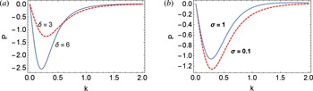
 $P$
is negative for all wavenumbers
 $k$
which is shown in figure 1. The coefficient of nonlinearity
 $Q$
given by
 $$\begin{eqnarray}\displaystyle Q & = & \displaystyle \frac{(\unicode[STIX]{x1D714}^{2}-\unicode[STIX]{x1D70E}k^{2})}{4\unicode[STIX]{x1D6FF}\unicode[STIX]{x1D714}k^{2}}(1+2A+2D)-Ek-\frac{\unicode[STIX]{x1D714}}{2}\left(k^{2}+\frac{1}{\unicode[STIX]{x1D6FF}}\right)^{2}\nonumber\\ \displaystyle & & \displaystyle -\,\frac{k^{2}}{\unicode[STIX]{x1D714}}A-B\frac{\unicode[STIX]{x1D714}^{2}+\unicode[STIX]{x1D70E}k^{2}}{2\unicode[STIX]{x1D714}}-\frac{(D+1)}{2\unicode[STIX]{x1D6FF}\unicode[STIX]{x1D714}}(\unicode[STIX]{x1D714}^{2}-\unicode[STIX]{x1D70E}k^{2}),\end{eqnarray}$$
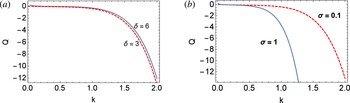
arises due to interaction among the waves and is related to the nonlinear frequency shift. For the present case,
 $Q$
is also negative for all values of
 $k$
, as shown in figure 2.
Variations of group dispersion coefficient
 $P$
with wavenumber
 $k$
for different plasma parameters. The plasma parameter are
 $(a)$
 $\unicode[STIX]{x1D70E}=0.1$
and
 $(b)$
 $\unicode[STIX]{x1D6FF}=3$
.

Variations of nonlinear coefficient
 $Q$
with wavenumber
 $k$
for different plasma parameters. The plasma parameters for the different panels are same as in figure 1.

The relation (3.14) clearly shows that
 $\unicode[STIX]{x1D6E4}$
depends on ion-neutral collisions
 $(\bar{\unicode[STIX]{x1D708}}_{in})$
as well as the ionization and ion loss rates
 $(\bar{\unicode[STIX]{x1D708}}_{L})$
. The term
 $\unicode[STIX]{x1D6E4}_{ion}$
is due to the creation of new ions by collisions of fast moving electrons with neutral particles. The term
 $\bar{\unicode[STIX]{x1D708}}_{L}$
originates from the loss of ions fluid due to attachment of ions on the dust grain surface. The process of attachment of the ions on the dust grain surface involves inelastic collisions in which the energy of the DIAW is lost and damping is introduced in the system. Charging of dust grains by attachment of electrons onto the grain surface also introduces damping in the same mechanism (Ghosh et al.
Reference Ghosh, Sarkar, Khan and Gupta2011, Reference Ghosh, Khan and Gupta2006b
). However, we did not consider that effect here for simplicity of the problem. The collisions between ions and neutral atoms also results in loss of energy of the ions, thus producing a damping effect. However, when ions are produced by collisions of fast moving electrons with neutral particles, energy is fed into the system of ion fluid and this energy triggers an instability known as the ionization instability. The dissipative term
 $\unicode[STIX]{x1D6E4}$
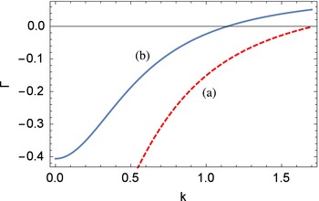
can be positive (damped) or negative (instability) for suitable values of plasma parameters, as shown in figure 3. Analytically, it can be shown that
 $\unicode[STIX]{x1D6E4}$
changes its sign in the following manner:
 $$\begin{eqnarray}\unicode[STIX]{x1D6E4}\gtrless 0\quad \text{according as}~\bar{\unicode[STIX]{x1D708}}_{in}+2\bar{\unicode[STIX]{x1D708}}_{L}\gtrless \unicode[STIX]{x1D6E4}_{ion}.\end{eqnarray}$$
This leads to the following condition:
 $$\begin{eqnarray}\displaystyle \unicode[STIX]{x1D6E4}\gtrless 0\quad \text{according as}~k^{2}\gtrless \frac{\bar{\unicode[STIX]{x1D708}}_{L}\bar{\unicode[STIX]{x1D6E9}}_{0}}{\bar{\unicode[STIX]{x1D708}}_{in}+2\bar{\unicode[STIX]{x1D708}}_{L}}-\frac{1}{\unicode[STIX]{x1D6FF}}, & & \displaystyle\end{eqnarray}$$
where
 $\bar{\unicode[STIX]{x1D6E9}}_{0}=(\text{d}\unicode[STIX]{x1D6E9}/\text{d}\unicode[STIX]{x1D719})_{0}/\unicode[STIX]{x1D6E9}_{0}$
. In the next section, we will see that a negative value of
 $\unicode[STIX]{x1D6E4}$
gives instability and a positive value of
 $\unicode[STIX]{x1D6E4}$
gives damping of the wave modes. In the absence of collisions, ion loss and ionization
 $(\unicode[STIX]{x1D6E4}=0)$
, we recover the usual NLSE for DIAW modulation (Amin et al.
Reference Amin, Morfill and Shukla1998).
Variations of
 $\unicode[STIX]{x1D6E4}$
with wavenumber
 $k$
for different plasma parameters with fixed
 $\unicode[STIX]{x1D6FF}=3$
. The plasma parameters are: (a)
 $\bar{\unicode[STIX]{x1D6E9}}_{0}=10$
and (b)
 $\bar{\unicode[STIX]{x1D6E9}}_{0}=5$
.

4 Modulational instability
In this section, we investigate the modulational characteristics of the DIAW for positive values of
 $\unicode[STIX]{x1D6E4}$
. From analogy with the quantum mechanical view point,
 $|\unicode[STIX]{x1D713}|^{2}$
in the above NLSE (equation (3.13)) with a linear dissipative term behaves like the potential for the propagating wave and this potential depends on
 $\unicode[STIX]{x1D713}$
itself, making it nonlinear. Actually, this nonlinearity is introduced in the system via the ponderomotive force which depends on the gradient of the wave intensity (
 $\unicode[STIX]{x1D735}|\unicode[STIX]{x1D713}|^{2}$
). The direction of this force is such that the particles will concentrate in a region where the wave amplitude is high. The local maxima of this potential energy acts as an effective potential well in the plasma. The low-frequency DIAW gets trapped within these potential wells created by the wave itself. The trapping of the wave further enhances the digging process of the well and instability is initiated in the system (Ablowitz & Suger Reference Ablowitz and Suger1981; Chen Reference Chen1990; Bellan Reference Bellan2011).
To study the instability, we have assumed that the amplitude evolution equation of the IAW (3.13) possesses the following plane wave solution
 $$\begin{eqnarray}\displaystyle \unicode[STIX]{x1D713}=\unicode[STIX]{x1D713}_{0}(\unicode[STIX]{x1D70F})\exp \left(-\text{i}\int _{0}^{\unicode[STIX]{x1D70F}}\unicode[STIX]{x1D6E5}(\unicode[STIX]{x1D70F}^{\prime })\,\text{d}\unicode[STIX]{x1D70F}^{\prime }\right), & & \displaystyle\end{eqnarray}$$
where
 $\unicode[STIX]{x1D713}_{0}(\unicode[STIX]{x1D70F})$
and
 $\unicode[STIX]{x1D6E5}(\unicode[STIX]{x1D70F})$
are the amplitude of the pump carrier wave and the nonlinear frequency shift in the presence of dissipation, respectively. Substitution of this plane wave solution into (3.13), yields the following two equations:
 $$\begin{eqnarray}\displaystyle \frac{\text{d}\unicode[STIX]{x1D713}_{0}}{\text{d}\unicode[STIX]{x1D70F}}+\unicode[STIX]{x1D6E4}\unicode[STIX]{x1D713}_{0}=0 & & \displaystyle\end{eqnarray}$$
and
 $$\begin{eqnarray}\displaystyle \unicode[STIX]{x1D6E5}(\unicode[STIX]{x1D70F})=-Q|\unicode[STIX]{x1D713}_{0}(\unicode[STIX]{x1D70F})|^{2}, & & \displaystyle\end{eqnarray}$$
which has solution of the following form:
 $\unicode[STIX]{x1D713}_{0}(\unicode[STIX]{x1D70F})=\unicode[STIX]{x1D713}_{00}\exp (-2\unicode[STIX]{x1D6E4}\unicode[STIX]{x1D70F})$
; where,
 $\unicode[STIX]{x1D713}_{00}$
is a real constant. Also note that for
 $\unicode[STIX]{x1D6E4}>0$
,
 $\unicode[STIX]{x1D713}_{0}(\unicode[STIX]{x1D70F})\rightarrow 0$
as
 $\unicode[STIX]{x1D70F}\rightarrow \infty$
which implies that
 $\unicode[STIX]{x1D713}_{0}$
is stable. But for
 $\unicode[STIX]{x1D6E4}<0$
,
 $\unicode[STIX]{x1D713}_{0}$
becomes unbounded (unstable) as
 $\unicode[STIX]{x1D70F}\rightarrow \infty$
and thereby the perturbation analysis is not appropriate. Therefore we restrict ourselves for
 $\unicode[STIX]{x1D6E4}>0$
. In this case, for the stability analysis, we consider the perturbation about
 $\unicode[STIX]{x1D713}_{0}(\unicode[STIX]{x1D70F})$
in the following standard procedure,
 $$\begin{eqnarray}\displaystyle \unicode[STIX]{x1D713}=[\unicode[STIX]{x1D713}_{0}(\unicode[STIX]{x1D70F})+\tilde{\unicode[STIX]{x1D713}}(\unicode[STIX]{x1D709},\unicode[STIX]{x1D70F})]\exp \left(-\text{i}\int _{0}^{\unicode[STIX]{x1D70F}}\unicode[STIX]{x1D6E5}(\unicode[STIX]{x1D70F}^{\prime })\,\text{d}\unicode[STIX]{x1D70F}^{\prime }\right), & & \displaystyle\end{eqnarray}$$
where
 $\tilde{\unicode[STIX]{x1D713}}(|\tilde{\unicode[STIX]{x1D713}}|\ll \unicode[STIX]{x1D713}_{0})$
is the perturbed amplitude of the modulated wave. After the substitution of (4.4) into (3.13) and following standard procedure (Ghosh et al.
Reference Ghosh, Sarkar, Khan and Gupta2011) one can show that the dispersion relation is given by
 $(\tilde{\unicode[STIX]{x1D714}}+\text{i}\unicode[STIX]{x1D6E4})^{2}=P^{2}\tilde{k}^{4}-2PQ|\unicode[STIX]{x1D713}_{0}|^{2}\tilde{k}^{2}$
.
This dispersion relation shows that for positive
 $\unicode[STIX]{x1D6E4}$
,
 $\unicode[STIX]{x1D714}$
becomes real, causing damping of the wave modes. Again, if we neglect the effect of
 $\unicode[STIX]{x1D6E4}$
, there is a possibility of the instability (imaginary
 $\unicode[STIX]{x1D714}$
) for
 $PQ>0$
(both
 $P$
and
 $Q$
are of negative sign in this case). In such a case, instability could occur if the wavenumber
 $k$
is smaller than a critical value
 $k_{cr}$
given by
 $$\begin{eqnarray}\displaystyle \tilde{k}^{2}<\tilde{k}_{cr}^{2}=\left(\frac{2Q}{P}\right)|\unicode[STIX]{x1D713}_{0}|^{2}=\left(\frac{2Q}{P}\right)|\unicode[STIX]{x1D713}_{00}|^{2}\exp (-2\unicode[STIX]{x1D6E4}\unicode[STIX]{x1D70F}). & & \displaystyle\end{eqnarray}$$
In the range 0 to
 $k_{cr}$
, instability may occur if the inequality
 $$\begin{eqnarray}\unicode[STIX]{x1D6E4}<\sqrt{P^{2}\tilde{k}^{2}\left(\frac{\tilde{k}_{cr}^{2}}{\tilde{k}^{2}}-1\right)}\end{eqnarray}$$
holds. Also, there is a time limit up to which the instability is observable and this time depends on the values of
 $P$
,
 $Q$
,
 $\tilde{k}$
and
 $\unicode[STIX]{x1D6E4}$
. The maximum time
 $\unicode[STIX]{x1D70F}_{max}$
to observe the instability is obtained from dispersion relation
 $$\begin{eqnarray}\displaystyle \unicode[STIX]{x1D70F}_{max}=\frac{1}{2\unicode[STIX]{x1D6E4}}\ln \left(\frac{2PQ\tilde{k}^{2}|\unicode[STIX]{x1D713}_{00}|^{2}}{\unicode[STIX]{x1D6E4}^{2}+P^{2}\tilde{k}^{4}}\right). & & \displaystyle\end{eqnarray}$$
The instability growth will cease after a time
 $t\geqslant \unicode[STIX]{x1D70F}_{max}$
.
5 Soliton solutions
In this section, we analytically solve the derived dissipative NLSE (equation (3.13)). In this NLSE, the group dispersion coefficient
 $P$
(equation (3.16)) and nonlinearity coefficient
 $Q$
(equation (3.17)) are negative for all wavenumbers
 $k$
. Therefore, we recast the NLSE (equation (3.13)) in the following normal form
 $$\begin{eqnarray}\displaystyle \text{i}\frac{\unicode[STIX]{x2202}\unicode[STIX]{x1D713}}{\unicode[STIX]{x2202}\bar{\unicode[STIX]{x1D70F}}}-\frac{1}{2}\frac{\unicode[STIX]{x2202}^{2}\unicode[STIX]{x1D713}}{\unicode[STIX]{x2202}\bar{\unicode[STIX]{x1D709}}^{2}}-|\unicode[STIX]{x1D713}|^{2}\unicode[STIX]{x1D713}+\text{i}\unicode[STIX]{x1D6FE}\unicode[STIX]{x1D713}=0, & & \displaystyle\end{eqnarray}$$
where,
 $\bar{\unicode[STIX]{x1D70F}}=|Q|\unicode[STIX]{x1D70F},\bar{\unicode[STIX]{x1D709}}=\unicode[STIX]{x1D709}\sqrt{|Q|/|P|}$
and
 $\unicode[STIX]{x1D6FE}=\unicode[STIX]{x1D6E4}/|Q|$
. In presence of
 $\unicode[STIX]{x1D6FE}$
, the equation (5.1) is a not completely integrable Hamiltonian system. As a result, the energy of the system is not conserved. Therefore, the energy equation of (5.1) is as follows:
 $$\begin{eqnarray}\displaystyle \frac{\text{d}{\mathcal{E}}}{\text{d}\bar{\unicode[STIX]{x1D70F}}}=-2\unicode[STIX]{x1D6FE}{\mathcal{E}},\quad \text{where}~{\mathcal{E}}=\int _{-\infty }^{\infty }|\unicode[STIX]{x1D713}(\bar{\unicode[STIX]{x1D709}},\bar{\unicode[STIX]{x1D70F}})|^{2}\,\text{d}\bar{\unicode[STIX]{x1D709}}. & & \displaystyle\end{eqnarray}$$
It is well known that the nonlinear Schrödinger equation (5.1) leads to the envelope solitons. From this energy equation, we can easily find the exact expression of soliton energy, which is as follows:
 $$\begin{eqnarray}\displaystyle {\mathcal{E}}={\mathcal{E}}(0)\exp (-2\unicode[STIX]{x1D6FE}\bar{\unicode[STIX]{x1D70F}}), & & \displaystyle\end{eqnarray}$$
where
 ${\mathcal{E}}(0)$
is the initial energy of the soliton. From the above equation we can conclude that for positive (negative)
 $\unicode[STIX]{x1D6FE}$
, the amplitude of the soliton decreases (increases) exponentially with decay (growth) rate
 ${\sim}2\unicode[STIX]{x1D6FE}$
as time increases. To study this in detail, we take an approximate solution of (5.1) for small
 $\unicode[STIX]{x1D6FE}$
which is in form of a solitary standing wave (Pereira & Stelnflo Reference Pereira and Stelnflo1977)
 $$\begin{eqnarray}\displaystyle \unicode[STIX]{x1D713}(\bar{\unicode[STIX]{x1D709}},\bar{\unicode[STIX]{x1D70F}})=\sqrt{2}\unicode[STIX]{x1D705}(\bar{\unicode[STIX]{x1D70F}})\text{sech}[\unicode[STIX]{x1D705}(\bar{\unicode[STIX]{x1D70F}})\bar{\unicode[STIX]{x1D709}}]\exp \left[\text{i}\int _{0}^{\bar{\unicode[STIX]{x1D70F}}}\unicode[STIX]{x1D705}^{2}(\acute{\unicode[STIX]{x1D70F}})\,\text{d}\acute{\unicode[STIX]{x1D70F}}\right]. & & \displaystyle\end{eqnarray}$$
The soliton amplitude and width are represented here through the single parameter
 $\unicode[STIX]{x1D705}(\bar{\unicode[STIX]{x1D70F}})$
which also determines the nonlinear frequency shift. Now, by substituting above solution (5.4) into (5.2), we obtain
 $$\begin{eqnarray}\displaystyle \frac{\text{d}\unicode[STIX]{x1D705}}{\text{d}\bar{\unicode[STIX]{x1D70F}}}=-2\unicode[STIX]{x1D6FE}\unicode[STIX]{x1D705}, & & \displaystyle\end{eqnarray}$$
From the above (5.5), we obtain the exact expression of
 $\unicode[STIX]{x1D705}(\bar{\unicode[STIX]{x1D70F}})$
as follows:
 $$\begin{eqnarray}\displaystyle \unicode[STIX]{x1D705}(\bar{\unicode[STIX]{x1D70F}})=\unicode[STIX]{x1D705}(0)\exp [-2\unicode[STIX]{x1D6FE}\bar{\unicode[STIX]{x1D70F}}], & & \displaystyle\end{eqnarray}$$
where
 $\unicode[STIX]{x1D705}(0)$
is the initial amplitude of the solitary wave. Now we present the analytical solution of (5.1) in the proceeding text in both case i.e.
 $\unicode[STIX]{x1D6E4}=0$
and
 $\unicode[STIX]{x1D6E4}\neq 0$
.
In the absence of ionization, ion loss and ion-neutral collisions in the system, we set the ion loss frequency and the collisional frequency both to zero, i.e.
 $\bar{\unicode[STIX]{x1D708}}_{in}=0=\bar{\unicode[STIX]{x1D708}}_{L}\Rightarrow \unicode[STIX]{x1D6E4}=0.$
Therefore, we can put
 $\unicode[STIX]{x1D6FE}=0$
in (5.1). Now we have the usual NLSE which is solved for negative dispersion and nonlinearity. We obtain the following exact single bright soliton which in terms of actual parameters looks as
 $$\begin{eqnarray}\displaystyle \unicode[STIX]{x1D713}(\unicode[STIX]{x1D709},\unicode[STIX]{x1D70F})=\sqrt{2}\unicode[STIX]{x1D705}(0)\text{sech}\left[\unicode[STIX]{x1D705}(0)\sqrt{\frac{|Q|}{|P|}}\unicode[STIX]{x1D709}\right]\exp \left[\text{i}\unicode[STIX]{x1D705}^{2}(0)|Q|\unicode[STIX]{x1D70F}\right]. & & \displaystyle\end{eqnarray}$$
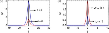
This solution shows that the soliton amplitude and width are constant with time and the exponential factor is responsible for the oscillation between maxima and minima. We represent this bright soliton graphically in figure 4 for different plasma parameters.
Bright envelope soliton with
 $\unicode[STIX]{x1D6E4}=0$
for the different plasma parameters of (3.13). The plasma parameters are: (a)
 $\unicode[STIX]{x1D70E}=0.1$
,
 $k=0.2$
and (b)
 $\unicode[STIX]{x1D6FF}=3$
.

In the presences of ionization, ion loss and ion-neutral collisions in the system of the dusty plasma,
 $\bar{\unicode[STIX]{x1D708}}_{L}\neq 0$
and
 $\bar{\unicode[STIX]{x1D708}}_{in}\neq 0$
therefore
 $\unicode[STIX]{x1D6E4}\neq 0$
. We obtain the following bright soliton (envelope soliton) in the presence of
 $\unicode[STIX]{x1D6E4}$
, which in terms of actual variable reads as
 $$\begin{eqnarray}\displaystyle \unicode[STIX]{x1D713}(\unicode[STIX]{x1D709},\unicode[STIX]{x1D70F}) & = & \displaystyle \sqrt{2}\unicode[STIX]{x1D705}(0)\exp (-2\unicode[STIX]{x1D6E4}\unicode[STIX]{x1D70F})\text{sech}\left[\unicode[STIX]{x1D705}(0)\exp (-2\unicode[STIX]{x1D6E4}\unicode[STIX]{x1D70F})\sqrt{\frac{|Q|}{|P|}}\unicode[STIX]{x1D709}\right]\nonumber\\ \displaystyle & & \displaystyle \times \,\exp \left[-\text{i}\frac{\unicode[STIX]{x1D705}^{2}(0)|Q|}{4\unicode[STIX]{x1D6E4}}[\exp (-4\unicode[STIX]{x1D6E4}\unicode[STIX]{x1D70F})-1]\right].\end{eqnarray}$$
In the limit
 $\unicode[STIX]{x1D6E4}\rightarrow 0$
, we recover the previous result in (5.7). This solution shows that for positive (negative)
 $\unicode[STIX]{x1D6E4}$
, the amplitude and width of the soliton decrease (increase) exponentially with the decay (growth) rate
 ${\sim}2\unicode[STIX]{x1D6E4}$
as time increases.
We have already discussed that
 $\unicode[STIX]{x1D6E4}$
changes its sign (positive/negative) depending upon the intensity of ionization and collisions. When the ion-neutral collisions and ion loss dominate over ionization, then
 $\unicode[STIX]{x1D6E4}$
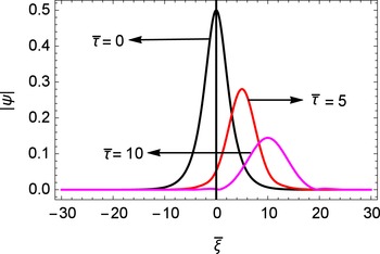
is positive, yielding the damped solition. From the analytical expression (5.8), we can see that for positive
 $\unicode[STIX]{x1D6E4}$
, as time elapses the amplitude of the bright (envelope) soliton decreases exponentially with decay rate
 ${\sim}2\unicode[STIX]{x1D6E4}$
. The numerical analysis also predicts the same results, as shown in the figure 5. So it is clear that positive
 $\unicode[STIX]{x1D6E4}$
i.e. when ion-neutral collisions and ion loss dominate over ionization, yields a damping effect on the bright soliton structure.
Bright soliton in the presence dissipation due to ionization, ion loss and ion-neutral collisions. Numerical solution of (5.1) for
 $\unicode[STIX]{x1D6E4}=0.1$
, where
 $\bar{\unicode[STIX]{x1D70F}}=|Q|\unicode[STIX]{x1D70F}$
and
 $\bar{\unicode[STIX]{x1D709}}=|Q|/2|P|$
.

On the other hand, when ionization dominates over ion-neutral collisions and ion loss,
 $\unicode[STIX]{x1D6E4}$
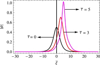
becomes negative. In this case, the amplitude of the modulated wave is amplified due to the ionization instability. The analytical solution (equation (5.8)) of the NLSE with the linear term
 $\unicode[STIX]{x1D6FE}$
(with negative sign) shows that, as time elapses, the amplitude of the bright (envelope) soliton increases exponentially with growth rate
 ${\sim}2\unicode[STIX]{x1D6E4}$
. Numerical solution also predicts qualitatively the same results, as shown in figure 6.
Bright soliton in the presence of ionization, ion loss and ion-neutral collisions. Numerical solution of (5.1) for
 $\unicode[STIX]{x1D6E4}=-0.1$
.

6 Numerical analysis
In the previous section we have seen that the solution of (3.13) with
 $\unicode[STIX]{x1D6E4}\neq 0$
is not exact as it is not an exactly integrable Hamiltonian system. Therefore, we are interested to find the effects of ionization and ion-neutral collisions on the nonlinear DIAW numerically. With the help of a MATHEMATICA based finite difference scheme, we have solved the numerical solution of (3.13) in both cases, i.e. NLSE with
 $\unicode[STIX]{x1D6E4}=0$
and
 $\unicode[STIX]{x1D6E4}\neq 0$
. The values of the physical parameters for the numerical computations are taken from dusty plasma experiments. The representative typical laboratory dusty plasma parameters are (D’Angelo Reference D’Angelo1997; Ghosh Reference Ghosh2006):
 $m_{i}=6.69\times 10^{-26}$
Kg,
 $T_{i}=0.3~\text{eV}$
,
 $n_{i0}\sim 10^{17}~\text{m}^{-3}$
,
 $T_{e}=3~\text{eV}$
and
 $\unicode[STIX]{x1D6FF}=3$
. These yield
 $\bar{\unicode[STIX]{x1D708}}_{L}=6.8\times 10^{-2}$
and
 $\bar{\unicode[STIX]{x1D708}}_{in}=7.2\times 10^{-2}$
, which justify the physical assumptions and the perturbation scaling (3.3). Figure 1 shows that for
 $\unicode[STIX]{x1D70E}=0.1$
(a) and for
 $\unicode[STIX]{x1D6FF}=3$
(b), we observed that there are no qualitative changes of
 $P$
, only quantitative changes and
 $P$
is always negative for all values of
 $k$
. Moreover, figure 2 shows that
 $Q$
is also always negative for all values of
 $k$
and there are no qualitative changes for
 $\unicode[STIX]{x1D70E}=0.1$
(a) and for
 $\unicode[STIX]{x1D6FF}=3$
(b), only quantitative changes. So,
 $P$
and
 $Q$
are both negative for all values of
 $k$
, i.e.
 $PQ>0$
for all values of
 $k$
and therefore the solution of (3.13) is modulationally unstable. On the other hand, for fixed
 $\unicode[STIX]{x1D6FF}=3$
, the variations of the damping or growth term
 $\unicode[STIX]{x1D6E4}$
with the wavenumber
 $k$
are depicted in figure 3 for two different values:
 $\bar{\unicode[STIX]{x1D6E9}}_{0}=10$
and
 $\bar{\unicode[STIX]{x1D6E9}}_{0}=5$
. From figure 3, we have observed that for the value of
 $\bar{\unicode[STIX]{x1D6E9}}_{0}=10$
,
 $\unicode[STIX]{x1D6E4}$
is negative, i.e. ionization due to the impacts of fast moving electrons with neutral particles dominates over the ion-neutral collisions and ion loss. Whereas, in next case (
 $\bar{\unicode[STIX]{x1D6E9}}_{0}=5$
), after a certain value of
 $k$
,
 $\unicode[STIX]{x1D6E4}$
is positive. Therefore, ion-neutral collisions and ion loss dominate over ionization of the system. The critical value of the wavenumber
 $k$
has been derived analytically in (3.19). The numerical solution of (3.13) exhibits a single bright or envelope solition for
 $\unicode[STIX]{x1D6E4}=0$
. The numerical solution in the absence of
 $\unicode[STIX]{x1D6E4}$
is plotted for different plasma parameters in figure 4. Figure 4(a) indicates that, for constant
 $\unicode[STIX]{x1D70E}~(=0.1)$
, the amplitude of the bright soliton increases according to the increase of
 $\unicode[STIX]{x1D6FF}$
, i.e. the increase of ion density with respect to electron density. Whereas figure 4(b) shows that, as the temperature of the electrons increases with the respect to the ion temperature, the amplitude of the bright solitons increases for fixed
 $\unicode[STIX]{x1D6FF}=3$
. It is obvious that the increase of soliton amplitude depends on the increase of ion density with respect to electron density or the increase of electron temperature with respect to ion temperature, as in the both case the energy of the soliton is increased. So, our results are consistent with the physical system. In the presence of
 $\unicode[STIX]{x1D6E4}$
, the solution of (3.13) would depend on time. Therefore, for time-dependent numerical simulations, we use the normalized form (5.1) of (3.13). For numerical solutions, we can use the single bright or envelope soliton as the initial waveform:
 $\unicode[STIX]{x1D713}(\bar{\unicode[STIX]{x1D709}},0)=a\,\text{sech}(ab\bar{\unicode[STIX]{x1D709}})\exp [-\text{i}b\bar{\unicode[STIX]{x1D709}}],\bar{\unicode[STIX]{x1D709}}\in [-L,L]$
, where
 $b=\sqrt{|Q|/|P|}$
,
 $a=\sqrt{(|P|k^{2}+\unicode[STIX]{x1D714})/|Q|}$
is the amplitude of the wave and
 $L$
is the spatial length. The boundary condition is:
 $\unicode[STIX]{x1D713}(L,\unicode[STIX]{x1D70F})=\unicode[STIX]{x1D713}(-L,\unicode[STIX]{x1D70F})$
. We have taken
 $L=30$
for appropriate results.
 $\unicode[STIX]{x1D6E4}>0$
corresponds to the damping of the wave, which is depicted in figure 5, which is clearly demonstrated by the exponential decay nature of the amplitude. The numerical solution yields the instability of the wave which is depicted in figure 6 for
 $\unicode[STIX]{x1D6E4}<0$
. This figure shows that, as time increases, the amplitude of the wave increases exponentially. Therefore, the numerical and analytical solutions predict the same nature of the wave.
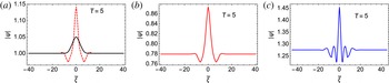
Time-dependent numerical simulations of (5.1). The numerical values of the parameters are
 $\unicode[STIX]{x1D713}_{00}=1$
,
 $\unicode[STIX]{x1D70E}=0.05$
and
 $\unicode[STIX]{x1D716}=0.05$
. (a) is drawn for no dissipation, (b) is drawn in the presence of dissipation with
 $\unicode[STIX]{x1D6FE}=0.05$
and (c) is drawn also in the presence of dissipation with
 $\unicode[STIX]{x1D6FE}=-0.05$
. In (a), the solid (black) curve is the initial perturbation pulse and the dotted curve (red) represents the typical profile of a bright Peregrine soliton at
 $\bar{\unicode[STIX]{x1D70F}}=5$
. (b,c) represent the same in the presence of dissipation.

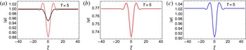
Time-dependent numerical simulations of (5.1). The numerical values of the parameters are
 $\unicode[STIX]{x1D713}_{00}=1$
;
 $\unicode[STIX]{x1D70E}=0.05$
and
 $\unicode[STIX]{x1D716}=0.05$
. (a) is drawn for no dissipation, (b) is drawn in the presence of dissipation with
 $\unicode[STIX]{x1D6FE}=0.05$
and (c) is drawn also in the presence of dissipation with
 $\unicode[STIX]{x1D6FE}=-0.05$
. In (a), the solid (black) curve is the initial perturbation pulse and the dotted curve (red) represents the typical profile of a dark or hole Peregrine soliton at
 $\bar{\unicode[STIX]{x1D70F}}=5$
. (b,c) represent the same in the presence of dissipation.

However, the rational solution of the NLSE contributes a major role to the theory of the rogue wave (Akhmediev & Ankiewicz Reference Akhmediev and Ankiewicz1997; Akhmediev, Ankiewicz & Soto-Crespo Reference Akhmediev, Ankiewicz and Soto-Crespo2009). The first-order rational solution is given by Peregrine (Peregrine Reference Peregrine1983) and is known as the Peregrine solution, which is localized in both space and time. Depending on the phase of the underlying carrier wave, the Peregrine soliton appears as bright Peregrine solitons and dark or hole Peregrine solitons (Peregrine Reference Peregrine1983). We have discussed here both of these. To know the effect of dissipation (damped/growth) numerically on the rogue wave solution, we consider the initial conditions of the rogue wave as a Gaussian-type perturbation pulse:
 $\unicode[STIX]{x1D713}(\bar{\unicode[STIX]{x1D709}},0)=\unicode[STIX]{x1D713}_{00}+\unicode[STIX]{x1D716}\exp [-\unicode[STIX]{x1D70E}\bar{\unicode[STIX]{x1D709}}^{2}],\bar{\unicode[STIX]{x1D709}}\in [-L,L]$
, where
 $\unicode[STIX]{x1D713}_{00}$
is the initial plane wave solution of the NLSE which is always positive,
 $\unicode[STIX]{x1D716}$
is a weak modulation amplitude,
 $\unicode[STIX]{x1D70E}$
is the inverse of the width of the initial perturbation and
 $L$
is the spatial length. For numerical simulation, we have fixed the parameter values as
 $\unicode[STIX]{x1D713}_{00}=1$
,
 $\unicode[STIX]{x1D70E}=0.05$
and
 $\unicode[STIX]{x1D716}=0.05$
. The results of the time-dependent numerical simulations of the normalized NLSE equation (5.1) are shown in figures 7 and 8. Figure 7(a) has been drawn in the absence of dissipation and this figure shows that at time
 $\bar{\unicode[STIX]{x1D70F}}=5$
, the maximum wave amplitude at
 $\bar{\unicode[STIX]{x1D709}}=0$
exceeds the modulated wave amplitude
 $(\unicode[STIX]{x1D716}=0.05)$
by a factor of three, i.e.
 $$\begin{eqnarray}|\unicode[STIX]{x1D713}(\bar{\unicode[STIX]{x1D709}}=0,\bar{\unicode[STIX]{x1D70F}}=5)-\unicode[STIX]{x1D713}_{00}|_{max}=0.15,\end{eqnarray}$$
which is the important characteristic of a bright Peregrine soliton (Peregrine Reference Peregrine1983). Figure 7(b) has been drawn in the presence of dissipation with
 $\unicode[STIX]{x1D6FE}=0.05$
. This figure shows the decreasing nature of the amplitude in the presence of dissipation with
 $\unicode[STIX]{x1D6FE}>0$
and yields the formation of a dissipative rogue wave. Whereas figure 7(c) shows the increasing nature of the amplitude in the presence of dissipation (growth) with
 $\unicode[STIX]{x1D6FE}=-0.05$
. In order to observe the dark or hole Peregrine soliton numerically, we have taken
 $\unicode[STIX]{x1D716}=-0.05$
and other parametric values are the same as used previously. Figure 8(a) has been drawn in the absence of dissipation and this figure shows that at time
 $\bar{\unicode[STIX]{x1D70F}}=5$
, the maximum wave amplitude at
 $\bar{\unicode[STIX]{x1D709}}=0$
exceeds the modulated wave amplitude
 $(\unicode[STIX]{x1D716}=0.05)$
by a factor of two, i.e.
 $$\begin{eqnarray}|\unicode[STIX]{x1D713}(\bar{\unicode[STIX]{x1D709}}=0,\bar{\unicode[STIX]{x1D70F}}=5)-\unicode[STIX]{x1D713}_{00}|_{max}=0.10,\end{eqnarray}$$
which is the important characteristic of a dark or hole Peregrine soliton (Chabchoub et al.
Reference Chabchoub, Neumann, Hoffmann and Akhmediev2012). Figure 8(b) shows the decreasing nature of the amplitude in the presence of dissipation (damped) with
 $\unicode[STIX]{x1D6FE}=0.05$
whereas figure 8(c) shows the increasing nature of the amplitude in the presence of dissipation (growth) with
 $\unicode[STIX]{x1D6FE}=-0.05$
.
7 Conclusion
In this paper, we have investigated the propagation of nonlinear ion acoustic wave modulations in a partially ionized dusty plasma composed of ions, electrons, dust grains and neutral particles. To incorporate the effect of ion-neutral collisions, ionization and ion loss, we have assumed that the ion-neutral and ion loss frequencies are very much smaller than the ion plasma frequency. We have taken the fluid model to describe the dynamics of ions whereas the electrons are Boltzmann distributed and the dust grains form a charge neutral background. The dynamics of nonlinear modulated IAW has been governed by the NLSE with a linear dissipative term (damped/growth) by using RPT. The linear dissipative term (damping or growth)
 $\unicode[STIX]{x1D6E4}$
arises due the ion-neutral collisions, ion attachment on dust grains (ion loss) and impact of fast moving electron on neutral particles (ionization). When the combines effects of ion-neutral collisions and ion loss dominate over ionization, then
 $\unicode[STIX]{x1D6E4}>0$
. In the opposite case,
 $\unicode[STIX]{x1D6E4}$
could be negative. Whereas, the sign of both the dispersion (
 $P$
) and the nonlinearity (
 $Q$
) coefficient are always negative for all values of
 $k$
. In the absence of ionization, ion loss and ion-neutral collisions, the NLSE reveals single bright or envelope solitons analytically and numerically in the unstable region
 $PQ>0$
. In the presence of the linear term the NLSE shows damped solitons for positive
 $\unicode[STIX]{x1D6E4}$
. Both analytical and numerical analyses exhibit damped solitons whose amplitudes decay exponentially with time. In the case of
 $\unicode[STIX]{x1D6E4}<0$
, the amplitude of the solitons increase exponentially as time increases, which leads to an instability of the wave known as the ionization instability. In other words, damping of solitons occurs due to the dominating effect of ion-neutral collisions and ion loss over ionization. Whereas the dominating effect of ionization over the combines effects of ion-neutral collisions and ion loss leads to the instability of the wave. Lastly, we have shown the effect of dissipation (damped/growth) on the rogue wave solution numerically.
Appendix A. Outlines of the calculations
Substitution of (3.1)–(3.2) into (2.3)–(2.5) yields the following
 $n^{th}$
-order reduced set of equations:
 $$\begin{eqnarray}\displaystyle & & \displaystyle \text{i}l(-\unicode[STIX]{x1D714}n_{l}^{(n)}+kv_{l}^{(n)})+\frac{\unicode[STIX]{x2202}}{\unicode[STIX]{x2202}\unicode[STIX]{x1D709}}(-v_{g}n_{l}^{(n-1)}+v_{l}^{(n-1)})+\frac{\unicode[STIX]{x2202}n_{l}^{(n-2)}}{\unicode[STIX]{x2202}\unicode[STIX]{x1D70F}}\nonumber\\ \displaystyle & & \displaystyle \qquad +\mathop{\sum }_{n^{\prime }=1}^{\infty }\mathop{\sum }_{l^{\prime }=-\infty }^{\infty }\left[\frac{\unicode[STIX]{x2202}}{\unicode[STIX]{x2202}\unicode[STIX]{x1D709}}(n_{l-l^{\prime }}^{(n-n^{\prime }-1)}v_{l^{\prime }}^{(n^{\prime })})+\text{i}kl\,n_{l-l^{\prime }}^{(n-n^{\prime })}v_{l^{\prime }}^{(n^{\prime })}\right]\nonumber\\ \displaystyle & & \displaystyle \quad =\overline{\unicode[STIX]{x1D708}}_{l}\left[\frac{1}{\unicode[STIX]{x1D6E9}}_{0}\left(\frac{\text{d}\unicode[STIX]{x1D6E9}}{\text{d}\unicode[STIX]{x1D719}}\right)_{0}\unicode[STIX]{x1D719}_{l}^{(n-2)}-n_{l}^{(n-2)}\right]\end{eqnarray}$$
 $$\begin{eqnarray}\displaystyle & & \displaystyle -\text{i}\unicode[STIX]{x1D714}lv_{l}^{(n)}+\text{i}kl\unicode[STIX]{x1D719}_{l}^{(n)}+\text{i}\unicode[STIX]{x1D70E}kln_{l}^{(n)}+(\bar{\unicode[STIX]{x1D708}}_{L}+\bar{\unicode[STIX]{x1D708}}_{in})v_{l}^{(n-2)}\nonumber\\ \displaystyle & & \displaystyle \qquad -\,v_{g}\frac{\unicode[STIX]{x2202}v_{l}^{(n-1)}}{\unicode[STIX]{x2202}\unicode[STIX]{x1D709}}+\unicode[STIX]{x1D70E}\frac{\unicode[STIX]{x2202}n_{l}^{(n-1)}}{\unicode[STIX]{x2202}\unicode[STIX]{x1D709}}-\frac{\unicode[STIX]{x2202}\unicode[STIX]{x1D719}_{l}^{(n-1)}}{\unicode[STIX]{x2202}\unicode[STIX]{x1D709}}+\frac{\unicode[STIX]{x2202}v_{l}^{(n-2)}}{\unicode[STIX]{x2202}\unicode[STIX]{x1D70F}}\nonumber\\ \displaystyle & & \displaystyle \quad =\mathop{\sum }_{n^{\prime }=1}^{\infty }\mathop{\sum }_{l^{\prime }=-\infty }^{\infty }\left[(v_{l-l^{\prime }}^{(n-n^{\prime }-1)}-v_{g}n_{l-l^{\prime }}^{(n-n^{\prime }-1)})\frac{\unicode[STIX]{x2202}v_{l^{\prime }}^{(n^{\prime })}}{\unicode[STIX]{x2202}\unicode[STIX]{x1D709}}\right.\nonumber\\ \displaystyle & & \displaystyle \qquad +\,\text{i}l^{\prime }(kv_{l-l^{\prime }}^{(n-n^{\prime })}v_{l^{\prime }}^{(n^{\prime })}-\unicode[STIX]{x1D714}n_{l-l^{\prime }}^{(n-n^{\prime })}v_{l^{\prime }}^{(n^{\prime })}+kn_{l-l^{\prime }}^{(n-n^{\prime })}\unicode[STIX]{x1D719}_{l^{\prime }}^{(n^{\prime })})\nonumber\\ \displaystyle & & \displaystyle \qquad \left.+\,n_{l-l^{\prime }}^{(n-n^{\prime }-1)}\frac{\unicode[STIX]{x2202}\unicode[STIX]{x1D719}_{l^{\prime }}^{(n^{\prime })}}{\unicode[STIX]{x2202}\unicode[STIX]{x1D709}}\right]\nonumber\\ \displaystyle & & \displaystyle \qquad -\mathop{\sum }_{n^{\prime \prime }=1}^{\infty }\mathop{\sum }_{l^{\prime \prime }=-\infty }^{\infty }\mathop{\sum }_{n^{\prime }=1}^{\infty }\mathop{\sum }_{l^{\prime }=-\infty }^{\infty }n_{l-l^{\prime }-l^{\prime \prime }}^{(n-n^{\prime }-n^{\prime \prime })}v_{l^{\prime }}^{(n^{\prime })}v_{l^{\prime \prime }}^{(n^{\prime \prime })}\end{eqnarray}$$
 $$\begin{eqnarray}\displaystyle & & \displaystyle \left[\frac{\unicode[STIX]{x2202}^{2}\unicode[STIX]{x1D719}_{l}^{(n-2)}}{\unicode[STIX]{x2202}\unicode[STIX]{x1D709}^{2}}+2\text{i}kl\frac{\unicode[STIX]{x2202}\unicode[STIX]{x1D719}_{l}^{(n-1)}}{\unicode[STIX]{x2202}\unicode[STIX]{x1D709}}-k^{2}l^{2}\unicode[STIX]{x1D719}_{l}^{(n)}\right]\nonumber\\ \displaystyle & & \displaystyle \quad =\frac{1}{\unicode[STIX]{x1D6FF}}\unicode[STIX]{x1D719}_{l}^{(n)}-n_{l}^{(n)}+\frac{1}{2}\mathop{\sum }_{n^{\prime }=1}^{\infty }\mathop{\sum }_{l^{\prime }=-\infty }^{\infty }\frac{1}{\unicode[STIX]{x1D6FF}}\unicode[STIX]{x1D719}_{l-l^{\prime }}^{(n-n^{\prime })}\unicode[STIX]{x1D719}_{l^{\prime }}^{(n^{\prime })}\nonumber\\ \displaystyle & & \displaystyle \qquad +\,\frac{1}{6}\frac{1}{\unicode[STIX]{x1D6FF}}\mathop{\sum }_{n^{\prime }=1}^{\infty }\mathop{\sum }_{l^{\prime }=-\infty }^{\infty }\mathop{\sum }_{n^{\prime \prime }=1}^{\infty }\mathop{\sum }_{l^{\prime \prime }=-\infty }^{\infty }\unicode[STIX]{x1D719}_{l-l^{\prime }-l^{\prime \prime }}^{(n-n^{\prime }-n^{\prime \prime })}\unicode[STIX]{x1D719}_{l^{\prime }}^{(n^{\prime })}\unicode[STIX]{x1D719}_{l^{\prime \prime }}^{(n^{\prime \prime })}.\end{eqnarray}$$
Appendix B. Expressions of different constants
 $$\begin{eqnarray}\displaystyle & \displaystyle A=\frac{1}{6k^{2}}\left[2\unicode[STIX]{x1D70E}\left(k^{2}+\frac{1}{\unicode[STIX]{x1D6FF}}\right)^{3}+3\left(k^{2}+\frac{1}{\unicode[STIX]{x1D6FF}}\right)^{2}-\frac{1}{\unicode[STIX]{x1D6FF}}\right] & \displaystyle\end{eqnarray}$$
 $$\begin{eqnarray}\displaystyle & \displaystyle B=\left(4k^{2}+\frac{1}{\unicode[STIX]{x1D6FF}}\right)A+\frac{1}{2\unicode[STIX]{x1D6FF}} & \displaystyle\end{eqnarray}$$
 $$\begin{eqnarray}\displaystyle & \displaystyle C=\frac{\unicode[STIX]{x1D714}}{k}(4k^{2}+\frac{1}{\unicode[STIX]{x1D6FF}})A+\frac{\unicode[STIX]{x1D714}}{k}\left[\frac{1}{2\unicode[STIX]{x1D6FF}}-\left(k^{2}+\frac{1}{\unicode[STIX]{x1D6FF}}\right)^{2}\right] & \displaystyle\end{eqnarray}$$
 $$\begin{eqnarray}\displaystyle & \displaystyle D=\frac{1}{(\unicode[STIX]{x1D6FF}+\unicode[STIX]{x1D70E}-v_{g}^{2})}\Bigg[v_{g}^{2}-2\unicode[STIX]{x1D70E}\unicode[STIX]{x1D6FF}\left(k^{2}+\frac{1}{\unicode[STIX]{x1D6FF}}\right)^{2}-k^{2}\unicode[STIX]{x1D6FF}-\unicode[STIX]{x1D70E}-3\Bigg] & \displaystyle\end{eqnarray}$$
 $$\begin{eqnarray}\displaystyle & \displaystyle E=\frac{v_{g}}{\unicode[STIX]{x1D6FF}}\left(D+1\right)-\frac{2\unicode[STIX]{x1D714}}{k}\left(k^{2}+1/\unicode[STIX]{x1D6FF}\right). & \displaystyle\end{eqnarray}$$