





1. Introduction
Pokrovski’s experiment is a simple configuration in which impact-induced acceleration of a liquid generates a focused jet from a gas–liquid interface (Lavrentiev & Chabat Reference Lavrentiev and Chabat1980; Antkowiak et al. Reference Antkowiak, Bremond, Dizès and Villermaux2007). In the classical configuration, a test tube partially filled with liquid falls freely and impacts a rigid substrate (see figure 1). During free fall, the gas–liquid interface inside the tube becomes concave because of surface tension in a reference frame where gravity is negligible. Upon impact, the liquid is rapidly accelerated, and the flow focuses at the concave interface, producing a focused jet (see figure 2 a). If the interface is flat just before impact, then by contrast, no jet is formed (Antkowiak et al. Reference Antkowiak, Bremond, Dizès and Villermaux2007). It is known that jets can be generated even when the container bottom is flat or further concave in shape (Lavrentiev & Chabat Reference Lavrentiev and Chabat1980); however, changes in the contact force profile caused by the container geometry can affect the jet velocity. In the present study, as discussed later, the contact force was modelled based on the convex hemispherical shape of the container bottom, by treating the problem as a sphere–substrate contact problem.
For rigid substrates, the dynamics of Pokrovski’s experiment has been described mainly using pressure-impulse theory. Antkowiak et al. (Reference Antkowiak, Bremond, Dizès and Villermaux2007) showed that the acoustic time scale is much shorter than the impact duration, so the liquid motion during impact can be treated as incompressible and governed by a momentum balance. Kiyama et al. (Reference Kiyama, Noguchi and Tagawa2014) proposed a semi-empirical formula for the jet velocity based on pressure-impulse theory and the focusing effect of a concave gas–liquid interface (Tagawa et al. Reference Tagawa, Oudalov, Visser, Peters, van der Meer, Sun, Prosperetti and Lohse2012; Peters et al. Reference Peters, Tagawa, Oudalov, Sun, Prosperetti, Lohse and van der Meer2013). Subsequent studies clarified how the pressure-impulse gradient, interface geometry and viscous effects influence the jet velocity (Krishnan et al. Reference Krishnan, Bharadwaj and Vasan2022; Cheng et al. Reference Cheng, Chen, Ding, Zhang, Hu and Jia2024; Watanabe et al. Reference Watanabe, Kusuno and Tagawa2025; Miyoshi et al. Reference Miyoshi, Watanabe, Kikuchi and Tagawa2026). In particular, Onuki et al. (Reference Onuki, Oi and Tagawa2018) pointed out that jet formation can be understood in terms of two time scales: an impact interval, during which the impact-generated pressure-impulse gradient accelerates the liquid, and a focusing interval, during which the concave gas–liquid interface focuses the flow.
Pokrovski’s experiment has also been extended to softer substrates. Kurihara et al. (Reference Kurihara, Kiyama and Tagawa2025) varied the contact time between the container and substrate using metal, resin and rubber substrates, and showed that finite liquid-acceleration time affects the pressure-field development during impact. Related water-hammer problems with finite acceleration time have also been discussed by Michele & Sammarco (Reference Michele and Sammarco2025). These studies clarified the role of finite acceleration time during the impact interval. However, how substrate compliance affects the subsequent focusing interval and the resulting jet velocity remains unclear.
In this study, we extend Pokrovski’s experiment to substrates with widely varying elastic moduli in order to determine how substrate deformability modifies the impulse available to deform the concave gas–liquid interface (hereafter denoted as
 $I$
) and, ultimately, the velocity of the focused jet. Here, we define the impact interval as the duration for which the container and substrate remain in contact, and the focusing interval as the time required for a jet to form from the concave interface. By varying the substrate elastic modulus over nearly six orders of magnitude, from
 $8.1\times 10^{-1}$
MPa to
 $2.0\times 10^{5}$
MPa, we access a regime in which the impact interval overlaps with the focusing interval. In this regime, the jet forms while the container is still in contact with the substrate, implying that the interface is not necessarily driven by the total impulse delivered over the full contact duration.
We show that the dimensionless jet velocity collapses when plotted against the Cauchy number
 $\textit{Ca}$
, and decreases markedly for
 $\textit{Ca}\gt 10^{-4}$
. We interpret this decrease as a partial-impulse effect: when the impact interval exceeds the focusing interval, only the impulse delivered within an effective time window set by the focusing dynamics contributes to jet acceleration. We formalise this idea by combining momentum conservation over this effective impulse window with an elastic foundation contact model, providing a quantitative description of jet velocities across both rigid and compliant substrates.
This paper is organised as follows. In § 2, we describe the experimental set-up and the data analysis. In § 3.1, we present the observed dependence of the jetting dynamics on substrate stiffness. In § 3.2, we show that the dimensionless jet velocity is organised by the Cauchy number
 $\textit{Ca}$
. In § 3.3, we develop the partial-impulse framework and compare the resulting model with the experimental results. In § 4, we summarise the main conclusions.
2. Experimental set-up
To investigate how a soft substrate affects the impulse
 $I$
used to deform a concave gas–liquid interface, we conducted Pokrovski’s experiment using nine substrates with different elastic moduli. Figure 1 shows the experimental set-up. First, a test tube (Maruemu, A-16.5, inner diameter 14.3 mm, outer diameter 16.5 mm) was filled with silicone oil of 10 cSt (Shin-Etsu Chemical, KF-96-10CS). Next, an aluminium plate with an iron S-shaped hook was attached to the top of the test tube using adhesive. The test tube was then placed on the substrate using an electromagnet (Fujita, round electromagnet FSGP-40). When the electromagnet was turned off, the test tube fell freely, and the gas–liquid interface was deformed by surface tension into a concave shape. After impact with the substrate, the interface deformed significantly, and a focused liquid jet was ejected. Two lights (HAYASHI-REPIC, LA-HDF158AA) were placed above the substrate to make it easier to observe the contact between the container and the substrate.
A schematic of the experimental set-up. A test tube filled with silicone oil of 10 cSt was released in free fall using an electromagnet to impact the substrate. The experimental parameters were the elastic modulus of the substrate
 $E$
, the impact velocity of the impactor
 $V_{{i}}=\sqrt {2gh_{\textit{drop}}}$
, and the liquid filling height
 $H$
. Here,
 $g = 9.81$
m s−
 $^2$
is the gravitational acceleration, and
 $h_{\textit{drop}}$
is the drop height. Nine substrates with different
 $E$
values, made of metals, resins, rubber and elastomers, were used.

Figure 1. Long description
Panel A: A schematic of the experimental setup. An electromagnet releases a test tube partially filled with silicone oil in free fall to impact a substrate. The setup includes a backlight, an electromagnet, an S-shaped hook, nine substrates with different elastic moduli, a marker, silicone oil, a high-speed camera, and lights. The impact velocity is determined by the drop height. Panel B: A diagram showing the different types of substrates used in the experiment, including metal, resin, rubber, and elastomer.
Table 1 summarises the substrate material, elastic modulus
 $E$
, and size and thickness
 $h$
, as well as the experimental conditions: the liquid filling height
 $H$
and the impact velocity
 $V_{{i}}$
of the impactor, which consisted of the test tube, the liquid, the aluminium plate and the S-shaped hook as a single unit. The experimental parameters were
 $V_{{i}}$
,
 $H$
and
 $E$
, where
 $V_{{i}}$
was varied from 0.63 m s−1 to 1.1 m s−1 by changing the drop height
 $h_{\textit{drop}}$
from 20 to 60 mm. Here,
 $V_{{i}}$
was calculated using
 $V_{{i}} = \sqrt {2gh_{\textit{drop}}}$
, where
 $g = 9.81$
m s−
 $^2$
is the gravitational acceleration. Height
 $H$
was used to change the mass of the impactor. For a rigid substrate, Kiyama et al. (Reference Kiyama, Tagawa, Ando and Kameda2016) reported that the pressure-impulse gradient generated in the liquid at impact does not depend on
 $H$
. Therefore, except when cavitation occurs, the jet velocity is independent of
 $H$
. In contrast, in this study, we examine the effect of
 $H$
on the jet velocity when
 $E$
is small. For the metal substrate,
 $H$
was set to 20 and 40 mm, while for the softer substrates with lower elasticity,
 $H$
was set to 20, 40 and 60 mm. For all settings for
 $H$
,
 $V_{{i}}$
and
 $E$
, we checked the high-speed images to confirm whether cavitation occurred, and no cavitation larger than one pixel was observed. Therefore, we concluded that no cavitation contributing to jet acceleration, as reported by Kiyama et al. (Reference Kiyama, Tagawa, Ando and Kameda2016), occurred in our experiments. Elastic modulus
 $E$
was varied from
 $8.1 \times 10^{-1}$
MPa to
 $2.0 \times 10^{5}$
MPa by using nine types of substrates, made of metal, resin, rubber and elastomer. For metal and resin substrates, the values of
 $E$
were taken from the literature (Ashby & Jones Reference Ashby and Jones2012; Yahamed et al. Reference Yahamed, Ikonomov, Fleming, Pekarovicova, Gustafson, Alden and Alfrafeek2016). The
 $E$
values of the rubber and elastomer substrates were determined experimentally by pressing a rigid sphere against the substrate surface (Yokoyama et al. Reference Yokoyama, Ichihara and Tagawa2024). In this experiment, the load applied to the substrate was measured as a function of the imposed surface displacement. We then obtained
 $E$
by applying an elastic foundation model that describes the relationship between the substrate displacement and the applied load (Johnson Reference Johnson1987); see Appendix A. We fabricated the elastomer substrates using polydimethylsiloxane (PDMS); see Appendix B. The elastic modulus of PDMS can be adjusted by changing the mass ratio of the base polymer (DOW, SILPOT 184 silicone elastomer base) to the curing agent (DOW, SILPOT 184 silicone elastomer curing agent) (Shukla et al. Reference Shukla, Higuita-Castro, Nana-Sinkam and Ghadiali2016). We used three types of PDMS substrates with mass ratios 10 : 1 (PDMS10), 20 : 1 (PDMS20) and 30 : 1 (PDMS30). To remove the stickiness of the PDMS substrate, baby powder (SiCCAROL-Hi, Asahi Group Foods Co. Ltd) was applied to eliminate surface adhesion.
A summary of the substrate materials, elastic moduli
 $E$
, sizes, and thicknesses
 $h$
, together with the values of the liquid filling height
 $H$
and impactor impact velocity
 $V_{{i}}$
for each substrate.

Table 1. Long description
A table with nine rows and six columns comparing different substrate materials, their elastic moduli, sizes, thicknesses, liquid filling heights, and impactor velocities. Column headers are Substrate, Material, E (M P A), Size (m m 2), h (m m), H (m m), and V i (m s 1). Row 1: SS400, Steel, 2.0 times 10 to the power of 5, 150 times 150, 20, 20 to 40, 0.63 to 1.1. Row 2: A5052, Aluminium, 6.9 times 10 to the power of 4, 150 times 150, 20, 20 to 40, 0.63 to 1.1. Row 3: Epoxy, Epoxy resin, 3.0 times 10 to the power of 3, 150 times 150, 20, 20 to 60, 0.63 to 1.1. Row 4: ABS, Acrylonitrile butadiene styrene resin, 1.9 times 10 to the power of 3, 150 times 150, 20, 20 to 60, 0.63 to 1.1. Row 5: PE, Polyethylene resin, 7.0 times 10 to the power of 2, 150 times 150, 20, 20 to 60, 0.63 to 1.1. Row 6: Rubber, Rubber, 1.9 times 10 to the power of 1, 150 times 150, 22.5, 20 to 60, 0.63 to 1.1. Row 7: PDMS10, Polydimethylsiloxane, 5.7 times 10 to the power of 0, 100 times 100, 22.0, 20 to 60, 0.63 to 1.1. Row 8: PDMS20, Polydimethylsiloxane, 1.7 times 10 to the power of 0, 100 times 100, 22.5, 20 to 60, 0.63 to 1.1. Row 9: PDMS30, Polydimethylsiloxane, 8.1 times 10 to the power of negative 1, 100 times 100, 22.0, 20 to 60, 0.63 to 1.1.
Images were captured using a high-speed camera (Photron, FASTCAM SA-X) with backlighting (PHLOX, white LED backlight
 $400 \times 200 \text{mm}^{2}$
). The frame rate of the camera was 10 000 fps, and the resolution was 0.160–0.169 mm pixel−1. The images were used to analyse the jet velocity, the time at which contact between the container and the substrate ended (
 $\tau _{\textit{impact}}$
), the time at which the centre of the interface rose due to flow focusing and the protrusion became visible from the side (
 $\tau _{\textit{focusing}}$
), and the gas–liquid interface thickness
 $H_{{m}}$
(as discussed in § 3.3.2). Here,
 $\tau _{\textit{focusing}}$
can be visually identified from the consecutive jet images in figure 4 below. The jet velocity was calculated from the relative position of the jet tip with respect to the test tube. The position of the test tube relative to the substrate was calculated using the printed marker on the test tube. For each experimental condition, the representative jet velocity
 $V_{\!{j}}$
was defined as the jet velocity at
 $t=\tau _{\textit{focusing}}$
(see § 3.1). Specifically, the change in the test tube rebound height,
 $\Delta h_{{t}}$
, and the change in the jet tip position,
 $\Delta h_{\!{j}}$
, were measured from two images taken at
 $t=\tau _{\textit{focusing}}$
and
 $t=\tau _{\textit{focusing}}+2\,\mathrm{ms}$
. The jet velocity was then calculated as
 $V_{\!{j}} = (\Delta h_{\!{j}}- \Delta h_{{t}})/\Delta t$
, where
 $\Delta t = 2\,\mathrm{ms}$
. Surface tension plays a crucial role in determining the initial meniscus shape. However, for the jet velocity immediately after jet formation considered in the present study, we confirmed that the capillary time scale is sufficiently longer than both
 $\tau _{\textit{impact}}$
and
 $\tau _{\textit{focusing}}$
. From the high-speed camera images, it was confirmed that the concave shape of the gas–liquid interface just before impact, which strongly affects the motion of the gas–liquid interface (Antkowiak et al. Reference Antkowiak, Bremond, Dizès and Villermaux2007), did not change significantly across all conditions. We also confirmed that the inclination of the test tube at impact was sufficiently small. This is because the test tube was suspended using a hook in a nearly point-contact configuration, which allowed the test tube, whose lower part was made heavier by the contained liquid, to align vertically under gravity and maintain an almost vertical orientation during the fall. The jet generation was repeated five times for each set of conditions.
3. Results and discussion
In this section, § 3.1 describes the typical interface motion and jet behaviour induced by impact onto substrates with various
 $E$
. We also discuss the relationship between the substrate elasticity and the jet velocity. In § 3.2, we show that the jet velocity can be described in a unified manner using the Cauchy number by organising the experimental results through dimensional analysis. In § 3.3, we clarify the mechanism of the reduced jet velocity on substrates with small
 $E$
by discussing the impulse
 $I$
used to deform a concave gas–liquid interface, and proposing a concept of a partial impulse.
3.1. Experimental observations of jet velocity reduction on soft substrates
In this subsection, we show that the jet velocity decreases as the substrate elasticity decreases. We also show that for softer substrates, the time required to deform the concave gas–liquid interface clearly increases. Figures 2(a) and 2(b) show the interface motion and the jet behaviour for
 $E = 2.0 \times 10^{5}$
and
 $8.1 \times 10^{-1}$
MPa at
 $H = 20$
mm and
 $V_{{i}} = 0.63$
m s−1. The time at which the container first makes contact with the substrate is defined as
 $t = 0$
ms, and the time interval between each image is 3 ms. Movies of the jet ejection are presented in the supplementary material is available at https://doi.org/10.1017/jfm.2026.11851. As mentioned in § 2, when the electromagnet was turned off, the impactor fell freely and impacted the substrate. Following the impact, the flow was focused by the concave gas–liquid interface, leading to the ejection and elongation of a focused liquid jet. At
 $t = 27$
ms, the jet tip was lower for
 $E = 8.1 \times 10^{-1}$
MPa than for
 $E = 2.0 \times 10^{5}$
MPa, which shows that the jet velocity was reduced. Furthermore, the time required for the concave interface to deform and generate a jet was longer for
 $E = 8.1 \times 10^{-1}$
MPa than for
 $E = 2.0 \times 10^{5}$
MPa. To quantify this difference, we investigated the time
 $t=\tau _{\textit{focusing}}$
when flow focusing was completed and the central part of the interface rose, making the protrusion visible from the side. At
 $E = 2.0 \times 10^{5}$
MPa,
 $\tau _{\textit{focusing}}=1.9$
ms, while at
 $E = 8.1 \times 10^{-1}$
MPa,
 $\tau _{\textit{focusing}}=5.7$
ms, which is approximately three times longer.
A comparison of the interface motion and jet behaviour for
 $H = 20$
mm and
 $V_{{i}} = 0.63$
m s−1, for (a)
 $E = 2.0 \times 10^{5}$
MPa, (b)
 $E = 8.1 \times 10^{-1}$
MPa. Here,
 $t = 0$
ms represents the time at which the container first makes contact with the substrate. For
 $E = 8.1 \times 10^{-1}$
MPa, the time required for the concave interface to deform is longer, and the jet tip position is lower, compared with
 $E = 2.0 \times 10^{5}$
MPa. (c) The time evolution of the jet velocity for different values of
 $E$
. Here,
 $t = 0$
ms represents the time at which the container first makes contact with the substrate; the plot starts at
 $t=\tau _{\textit{focusing}}$
and ends at the time of pinch-off. The results indicate that as
 $E$
decreases, the jet velocity becomes slower, while
 $\tau _{\textit{focusing}}$
increases.

Figure 2. Long description
Panel A: A series of photographs showing the motion of a liquid interface and jet formation in a test tube under an elastic modulus of 2.0 times 10 to the power of 5 megapascals. The photographs are taken at intervals of 3 milliseconds, starting from 0 milliseconds to 27 milliseconds. The liquid interface becomes concave during free fall and forms a jet upon impact with a rigid substrate. Panel B: A series of photographs similar to Panel A but under an elastic modulus of 8.1 times 10 to the power of -1 megapascals. The photographs show a slower deformation of the concave interface and a lower jet tip position compared to Panel A. Panel C: A line graph depicting the time evolution of jet velocity for different values of elastic modulus. The x-axis represents time in milliseconds, ranging from 0 to 50 milliseconds. The y-axis represents jet velocity in meters per second, ranging from 0 to 3 meters per second. The graph includes multiple lines, each representing a different elastic modulus value. The results indicate that as the elastic modulus decreases, the jet velocity becomes slower.
Figure 2(c) shows the time evolution of the jet velocity in 1 ms intervals for each
 $E$
at
 $H = 20$
mm and
 $V_{{i}} = 0.63$
m s−1. Here,
 $t = 0$
ms denotes the time at which the container first makes contact with the substrate; the plot starts at
 $t=\tau _{\textit{focusing}}$
and ends at the time of pinch-off. Each plot represents the average of five trials, and the error bars indicate the standard deviation. It is clearly observed that the jet velocity decreases as
 $E$
decreases. Looking at the starting points of the
 $t=\tau _{\textit{focusing}}$
plots for each
 $E$
,
 $\tau _{\textit{focusing}}$
increases with decreasing
 $E$
. Moreover, the ending points of the plots also increase as
 $E$
decreases, showing that the jet growth becomes slower. Focusing on the time evolution of the jet velocity, it reaches its maximum at approximately
 $t=\tau _{\textit{focusing}}$
, then converges to a constant value. In the following subsections, we use the representative jet velocity
 $V_{\!{j}}$
, defined as the jet velocity at
 $t=\tau _{\textit{focusing}}$
.
Next, we discuss the relationship between
 $V_{\!{j}}$
and
 $E$
. Figure 3(a) shows the relationship between
 $V_{\!{j}}$
and
 $E$
for all experimental conditions on a semi-log plot. Each plot represents the average of five trials, and the error bars indicate the standard deviation. Overall,
 $V_{\!{j}}$
tends to increase as
 $E$
increases, but the data points do not collapse onto a single curve. In more detail, when
 $V_{{i}}$
is fixed,
 $V_{\!{j}}$
increases with increasing
 $E$
, and when
 $E$
is fixed,
 $V_{\!{j}}$
increases with increasing
 $V_{{i}}$
. These results show that
 $V_{\!{j}}$
is strongly affected by both
 $E$
and
 $V_{{i}}$
. In the following subsections, we derive a dimensionless number that can describe the relationship between
 $V_{\!{j}}$
and
 $E$
in a unified manner using dimensional analysis.
(a) Plot of
 $V_{\!{j}}$
versus
 $E$
. Here,
 $V_{\!{j}}$
increases with increasing
 $E$
at fixed
 $V_{{i}}$
, and also increases with
 $V_{{i}}$
at fixed
 $E$
, indicating that
 $V_{\!{j}}$
strongly depends on both
 $E$
and
 $V_{{i}}$
. However, the data points do not collapse onto a single curve. (b) Plot of
 $V_{\!{j}}/V_{{i}}$
versus
 $\rho _{{e}}V_{{i}}^2/E$
. All data collapse onto a single curve. When
 $\rho _{{e}} V_{{i}}^2 / E\lt 10^{-4}$
, the variation in
 $V_{\!{j}}/V_{{i}}$
is small. Since this regime can be explained by the pressure-impulse theory established in previous studies using rigid substrates, we refer to it as the rigid-impact regime in this paper. In contrast, when
 $\rho _{{e}} V_{{i}}^2 / E \gt 10^{-4}$
,
 $V_{\!{j}}/V_{{i}}$
clearly decreases. This regime cannot be explained by conventional pressure-impulse theory. Because the influence of the soft substrate on the interfacial motion is pronounced, we refer to this region as the soft-impact regime. The black dashed line shows
 $V_{\!{j}}/V_{{i}} = 3.66$
estimated from the rigid substrate experiments by Kiyama et al. (Reference Kiyama, Tagawa, Ando and Kameda2016). The red line represents (3.11), while the black solid line represents the soft-limit asymptote of (3.11), given by (3.13), with slope
 $-1/4$
.

3.2. Jet velocity and Cauchy number: dimensional analysis
In this subsection, we use dimensional analysis to show that the experimental jet velocities can be unified using the Cauchy number. We also show that for a Cauchy number smaller than approximately
 $10^{-4}$
, the jet velocity can be described by the conventional pressure-impulse theory; this range is defined here as the rigid-impact regime. Furthermore, for a Cauchy number larger than approximately
 $10^{-4}$
, the jet velocity decreases in a way that cannot be explained by conventional pressure-impulse theory. In this regime, the influence of the soft substrate on the interfacial motion becomes pronounced; therefore, we define this regime as the soft-impact regime.
We use dimensional analysis to derive a dimensionless number that collapses the relationship between
 $V_{\!{j}}$
and
 $E$
. As mentioned above,
 $V_{\!{j}}$
is affected by
 $E$
and
 $V_{{i}}$
. This suggests that the contact dynamics, namely the temporal profile of the contact force exerted by the substrate on the impactor, including its magnitude, influences
 $V_{\!{j}}$
. In particular, in the present study, because the bottom of the impactor has a hemispherical shape with radius
 $R$
, where
 $R$
is the outer radius of the test tube, the parameters determining the contact-force profile can be considered based on the contact problem between a rigid sphere and a substrate. In this context, in addition to
 $V_{{i}}$
and
 $E$
, it is known that when a rigid sphere impacts a soft substrate, the sphere density is one of the parameters determining the type of contact, such as elastic or viscoelastic (Maruoka Reference Maruoka2023). Therefore,
 $V_{\!{j}}$
can be expressed as a function of
 $E$
,
 $V_{{i}}$
, and the effective density
 $\rho _{{e}}$
as
 \begin{equation} V_{\!{j}} = f(E, V_{{i}}, \rho _{{e}}). \end{equation}
Here,
 $\rho _{{e}}$
is calculated from
 $R$
and the impactor mass
 $m$
as
 \begin{equation} \rho _{{e}} = \frac {3m}{4 \pi R^3}, \end{equation}
which represents the density of a rigid sphere with the same outer radius
 $R$
as the test tube, and varies with
 $H$
in this experiment. Since both
 $R$
and the container geometry were fixed throughout the experiments, they were not directly incorporated as parameters in the dimensional analysis.
Dimensional analysis using the Buckingham
 $\varPi$
theorem yields
 \begin{equation} \frac {V_{\!{j}}}{V_{{i}}} =\varPhi \left(\frac {\rho _{{e}} V_{{i}}^2}{E}\right)\!, \end{equation}
where
 $V_{\!{j}}/V_{{i}}$
represents the dimensionless jet velocity, obtained by normalising
 $V_{\!{j}}$
with
 $V_{{i}}$
. Also,
 $\rho _{{e}} V_{{i}}^2 / E$
is a dimensionless number known as the Cauchy number, which represents the ratio of the impactor’s inertial force to the substrate’s elastic force. The dimensional analysis shows that
 $V_{\!{j}} / V_{{i}}$
can be described as a function of the Cauchy number.
We next investigate the relationship between
 $V_{\!{j}}/V_{{i}}$
and
 $\rho _{{e}}V_{{i}}^2/E$
in detail using the experimental data. Figure 3(b) shows the dependence of
 $V_{\!{j}}/V_{{i}}$
on
 $\rho _{{e}}V_{{i}}^2/E$
. Each plot represents the average of five trials, and the error bars indicate the standard deviation. Compared with figure 3(a), all the plots in figure 3(b) collapse onto a single curve. A key feature of the relationship between
 $V_{\!{j}}/V_{{i}}$
and
 $\rho _{{e}}V_{{i}}^2/E$
is that at
 $\rho _{{e}}V_{{i}}^2/E \sim 10^{-4}$
, the data separate into two regions: one where
 $V_{\!{j}}/V_{{i}}$
changes little, and another where it clearly decreases.
In the region where
 $\rho _{{e}}V_{{i}}^2/E\lt 10^{-4}$
, the value of
 $V_{\!{j}}/V_{{i}}$
changes only slightly. This behaviour can be explained using the results of Kiyama et al. (Reference Kiyama, Tagawa, Ando and Kameda2016), who reported the jet velocity in Pokrovski’s experiment with metal substrates. Kiyama et al. (Reference Kiyama, Tagawa, Ando and Kameda2016) reported that the dimensionless jet velocity
 $V_{\!{j}}/U_0$
, where
 $U_0$
is the velocity of the concave gas–liquid interface just after the impact, becomes
 $V_{\!{j}}/U_0 = 2.05$
when cavitation does not occur. We estimate
 $V_{\!{j}}/V_{{i}}$
from
 $V_{\!{j}}/U_0 = 2.05$
, as reported by Kiyama et al. (Reference Kiyama, Tagawa, Ando and Kameda2016), and compare it with our experimental data. Here,
 $U_0$
is defined as
 $U_0 = V_{{i}} + V_{{r}}$
, where
 $V_{{r}}$
is the rebound velocity of the impactor relative to the substrate (Kiyama et al. Reference Kiyama, Tagawa, Ando and Kameda2016). Because
 $V_{{r}}$
can be estimated as
 $ V_{{r}} \approx eV_{{i}}$
using the restitution coefficient
 $e$
,
 $U_0$
can be approximated by
 $U_0 \approx V_{{i}}(1 + e)$
. Therefore, to estimate
 $V_{\!{j}}/V_{{i}}$
from the value of
 $V_{\!{j}}/U_0$
reported by Kiyama et al. (Reference Kiyama, Tagawa, Ando and Kameda2016), we can use
 $V_{\!{j}}/V_{{i}} \approx V_{\!{j}}(1+e)/U_0$
. We obtained
 $e$
by analysing
 $V_{{r}}$
for the steel and aluminium substrates used in our experiments, and calculating
 $e = V_{{r}}/V_{{i}}$
to give
 $e = 0.787$
. We obtained
 $V_{{r}}$
using the same method as Kiyama et al. (Reference Kiyama, Tagawa, Ando and Kameda2016). We estimated
 $V_{\!{j}}/V_{{i}}$
from
 $V_{\!{j}}/U_0$
reported by Kiyama et al. (Reference Kiyama, Tagawa, Ando and Kameda2016), and obtained
 $V_{\!{j}}/V_{{i}} = 3.66$
. The black dashed line in figure 3(b) represents
 $V_{\!{j}}/V_{{i}} = 3.66$
. We find that the result of Kiyama et al. (Reference Kiyama, Tagawa, Ando and Kameda2016) captures the trend of
 $ V_{\!{j}}/V_{{i}}$
well in the region where
 $\rho _{{e}} V_{{i}}^2 / E\lt 10^{-4}$
in our experiments. This indicates that the jet velocity for
 $\rho _{{e}} V_{{i}}^2 / E\lt 10^{-4}$
can be explained by the theory established from Pokrovski’s experiments using metal substrates. So far, the impact of a ‘fluid-containing container’ on a rigid substrate has been modelled similarly to impacts between rigid bodies, using an incompressible-based approximation in which the total impulse from the substrate is transmitted almost instantaneously (Batchelor Reference Batchelor1967; Antkowiak et al. Reference Antkowiak, Bremond, Dizès and Villermaux2007; Kiyama et al. Reference Kiyama, Noguchi and Tagawa2014, Reference Kiyama, Tagawa, Ando and Kameda2016). The present results show that the applicability of this incompressible-based approximation can be evaluated using the Cauchy number. Furthermore, it is experimentally confirmed for the first time that the incompressible-based approximation is valid when
 $\rho _{{e}} V_{{i}}^2 / E\lt 10^{-4}$
. Therefore, in this study, the region
 $\rho _{{e}} V_{{i}}^2 / E\lt 10^{-4}$
is defined as the rigid-impact regime.
On the other hand, in the region where
 $\rho _{{e}} V_{{i}}^2 / E \gt 10^{-4}$
,
 $V_{\!{j}}/V_{{i}}$
decreases significantly with increasing Cauchy number. This region cannot be modelled using the incompressible-based approximation. In this study, we experimentally show for the first time that the effect of small
 $E$
becomes significant in fluid motion when
 $\rho _{{e}} V_{{i}}^2 / E \gt 10^{-4}$
. Therefore, we define the region
 $\rho _{{e}} V_{{i}}^2 / E \gt 10^{-4}$
as the soft-impact regime.
Since the rigid-impact regime and the soft-impact regime can be evaluated using the Cauchy number, these two regimes are determined not only by
 $E$
but also by the contact conditions, including
 $V_{{i}}$
and
 $\rho _{{e}}$
. However, under the present experimental conditions, the value of the Cauchy number is predominantly determined by
 $E$
. Therefore, the classification into the rigid-impact and soft-impact regimes can be readily made based on
 $E$
. In the present experiments, all data for
 $E \le 1.9 \times 10^{1}$
MPa are classified into the soft-impact regime, whereas all data for
 $E \ge 7.0 \times 10^{2}$
MPa fall within the rigid-impact regime. In the next subsection, we discuss the decrease of
 $V_{\!{j}}/V_{{i}}$
in the soft-impact regime, and clarify its underlying mechanism.
3.3. Mechanism of jet velocity reduction in the soft-impact regime
In this subsection, we elucidate the physical mechanism leading to the reduction of
 $V_{\!{j}}/V_{{i}}$
observed for the soft-impact regime. The key observation is the relative ordering of two time scales: the impact interval
 $\tau _{\textit{impact}}$
, during which the container and substrate remain in contact, and the focusing interval
 $\tau _{\textit{focusing}}$
, required for the concave gas–liquid interface to focus and produce a visible jet. For rigid substrates,
 $\tau _{\textit{impact}} \ll \tau _{\textit{focusing}}$
, so the contact force acts over a short interval, and the fluid subsequently focuses after the contact has ended. In this limit, it is natural to relate jetting to the total impulse delivered during contact.
For sufficiently soft substrates, however, we find
 $\tau _{\textit{impact}} \gt \tau _{\textit{focusing}}$
, meaning that jetting starts while contact is ongoing. In that case, the interface cannot be driven by the total impulse transmitted over the entire contact, because the jet forms before that impulse has been fully delivered. This motivates a framework in which the jet is controlled by the impulse accumulated up to the jet-formation time, i.e. the partial impulse. Below, we formalise this idea by (i) writing a momentum balance over the effective time window relevant for jet formation, and (ii) modelling the contact force history using an elastic foundation model.
3.3.1. Relative magnitude between the impact interval and the focusing interval
Figure 4 shows the evolution from the onset of impact to the stage where the jet elongates to approximately the test tube diameter for the conditions
 $H = 20$
mm and
 $V_{{i}} = 0.63$
m s−1, using seven images at equal time intervals. Figures 4(a–c) correspond to
 $ E = 2.0 \times 10^{5}$
,
 $1.7 \times 10^{0}$
and
 $8.1 \times 10^{-1}$
MPa, respectively. The time
 $t = 0$
ms denotes when the container begins to contact the substrate. The time when the container separates from the substrate is defined as
 $t = \tau _{\textit{impact}}$
. In this subsubsection,
 $t=\tau _{\textit{impact}}$
is interpreted as the time when the impact interval ends, and
 $t=\tau _{\textit{focusing}}$
as the time when the focusing interval ends, namely when the centre of the interface rises and a protrusion becomes visible from the side (see
 ). The values of
 $t = \tau _{\textit{impact}}$
and
 $t=\tau _{\textit{focusing}}$
were determined by analysing the complete image sequences recorded at intervals of 0.1 ms for all experiments. Among the seven equally time-spaced images displayed in figure 4, the images whose time stamps are closest to the evaluated values of
 $t = \tau _{\textit{impact}}$
and
 $t=\tau _{\textit{focusing}}$
are indicated by (
 $\color {red}{\blacktriangle }$
) and (
 ), respectively. Here, we focus on the relative magnitudes of
 $\tau _{\textit{impact}}$
and
 $\tau _{\textit{focusing}}$
. In the rigid-impact regime, for
 $E = 2.0 \times 10^{5}$
MPa,
 $\tau _{\textit{impact}} = 0.2$
ms and
 $\tau _{\textit{focusing}} = 1.9$
ms, giving
 $\tau _{\textit{impact}} \ll \tau _{\textit{focusing}}$
(see figure 4
a). This means that the impact interval is shorter than the focusing interval, and the jet forms after contact has ended. In contrast, in the soft-impact regime, the order of
 $\tau _{\textit{impact}}$
and
 $\tau _{\textit{focusing}}$
is reversed. For
 $E = 1.7 \times 10^{0}$
MPa,
 $\tau _{\textit{impact}} = 6.5$
ms and
 $\tau _{\textit{focusing}} = 5.0$
ms. For
 $E = 8.1 \times 10^{-1}$
MPa,
 $\tau _{\textit{impact}} = 9.2$
ms and
 $\tau _{\textit{focusing}} = 5.7$
ms, and in both cases,
 $\tau _{\textit{impact}} \gt \tau _{\textit{focusing}}$
. This means that the impact interval is longer than the focusing interval, and the jet is formed during the contact (see figures 4
b,c). The key point is that as
 $E$
decreases, the relationship between
 $\tau _{\textit{impact}}$
and
 $\tau _{\textit{focusing}}$
is reversed, and the impact interval becomes longer than the focusing interval. This suggests that in the soft-impact regime, the total impulse from the substrate to the container is not fully transmitted to the concave gas–liquid interface before the jet is formed.
The moments when the container separates from the substrate (see
 $\color {red}{\blacktriangle }$
) and when the centre of the interface rises and the protrusion becomes visible from the side (see
 ) are shown for (a)
 $E = 2.0 \times 10^{5}$
MPa, (b)
 $E = 1.7 \times 10^{0}$
MPa and (c)
 $E = 8.1 \times 10^{-1}$
MPa (
 $H = 20$
mm and
 $ V_{{i}} = 0.63$
m s−1). Here,
 $t = 0$
ms denotes the time when the container begins to make contact with the substrate. For
 $E = 2.0 \times 10^{5}$
MPa,
 $\tau _{\textit{impact}} = 0.2$
ms and
 $\tau _{\textit{focusing}} = 1.9$
ms, giving
 $\tau _{\textit{impact}} \ll \tau _{\textit{focusing}}$
. In other words, the impact interval is short compared to the focusing interval. In contrast, for
 $E = 1.7 \times 10^{0}$
and
 $8.1 \times 10^{-1}$
MPa, the centre of the interface rises, and the protrusion becomes visible from the side while the container and the substrate are in contact. In other words, the impact interval becomes longer than the focusing interval. Here,
 $H_{{m}}$
represents the meniscus thickness just before the container and the substrate come into contact.

Figure 4. Long description
Panel A: A series of photos showing the impact and focusing intervals of a liquid in a container with an elastic modulus of 2.0 times 10 to the power of 5 megapascals. The images capture the liquid’s behavior at different time intervals, from 0 to 4.2 milliseconds. The impact interval is marked in red and lasts for 0.2 milliseconds, while the focusing interval is marked in blue and lasts for 1.9 milliseconds. A close-up image shows the frame closest to the moment when the container separates from the substrate. Panel B: A series of photos showing the impact and focusing intervals of a liquid in a container with an elastic modulus of 1.7 times 10 to the power of 0 megapascals. The images capture the liquid’s behavior at different time intervals, from 0 to 10.2 milliseconds. The impact interval is marked in red and lasts for 6.5 milliseconds, while the focusing interval is marked in blue and lasts for 5.0 milliseconds. A close-up image shows the frame closest to the moment when the container separates from the substrate. Panel C: A series of photos showing the impact and focusing intervals of a liquid in a container with an elastic modulus of 8.1 times 10 to the power of -1 megapascals. The images capture the liquid’s behavior at different time intervals, from 0 to 12 milliseconds. The impact interval is marked in red and lasts for 9.2 milliseconds, while the focusing interval is marked in blue and lasts for 5.7 milliseconds. A close-up image shows the frame closest to the moment when the container separates from the substrate.
3.3.2. Development of a new model equation for the jet velocity
To discuss the mechanism behind the decrease in
 $V_{\!{j}}/V_{{i}}$
on soft substrates, we model the jet velocity in terms of the impulse transmitted from the substrate during the time that is dynamically relevant for formation. In Pokrovski’s experiment, the impact generates a force on the container over a finite duration, which initiates the motion of the concave gas–liquid interface and is subsequently amplified by flow focusing (Antkowiak et al. Reference Antkowiak, Bremond, Dizès and Villermaux2007; Kiyama et al. Reference Kiyama, Noguchi and Tagawa2014). In the rigid-impact regime, the contact ends well before the jet forms, and it is therefore natural to relate the jet to the total impulse delivered during the contact. In the soft-impact regime, however, we observe
 $\tau _{\textit{impact}} \gt \tau _{\textit{focusing}}$
, meaning that the jet forms while contact is still ongoing. In this case, the interface cannot be driven by the total impulse accumulated over the entire contact duration; instead, jet formation can only depend on the impulse delivered up to the end of the focusing interval.
(a) A schematic of the impactor and substrate at
 $t = 0$
and
 $t = \tau _{\textit{focusing}}$
. Here,
 $V'$
denotes the velocity of the impactor at
 $t = \tau _{\textit{focusing}}$
. In this study,
 $F$
is evaluated using an elastic foundation model, in which the elastic response of the substrate is modelled as a spring. (b) The time evolution of
 $F$
for each
 $E$
, obtained from the elastic foundation model for
 $H = 20$
mm and
 $V_{{i}} = 0.63$
m s−1. The shaded area represents
 $I$
calculated from (3.11), i.e. the effective impulse time window. For
 $E \ge 7.0 \times 10^{2}$
MPa, which falls within the rigid-impact regime, the jet is driven by
 $I$
obtained by integrating
 $F$
over its entire duration, i.e. the total impulse. In contrast, for
 $E \le 1.9 \times 10^{1}$
MPa, which belongs to the soft-impact regime, the jet is driven by the impulse
 $I$
obtained from a partial integration of
 $F$
, corresponding to a partial impulse.

This idea can be expressed without introducing additional variables by integrating the contact force over a finite time window. Importantly, this formulation automatically recovers the rigid-impact limit. When
 $\tau _{\textit{impact}} \lt \tau _{\textit{focusing}}$
, the contact force vanishes for
 $t \gt \tau _{\textit{impact}}$
, thus integrating up to
 $t=\tau _{\textit{focusing}}$
is equivalent to integrating over the full contact. In contrast, when
 $\tau _{\textit{impact}} \gt \tau _{\textit{focusing}}$
, the upper limit
 $t=\tau _{\textit{focusing}}$
cuts off the force history, so that only a portion of the total impulse contributes to jet formation (see figures 5(b) and 6). In the remainder of this section, we translate this concept into a predictive model by combining momentum conservation with a contact-force model based on the elastic foundation model.
We consider the motion of the impactor of mass
 $m$
over the interval from first contact,
 $t = 0$
, to the end of the focusing interval,
 $t = \tau _{\textit{focusing}}$
. Figure 5(a) shows a schematic of the impactor and the substrate over the time interval
 $[0,\tau _{\textit{focusing}}]$
. Let
 $F(t)$
denote the magnitude of the normal contact force exerted by the substrate on the container. Over
 $[0,\tau _{\textit{focusing}}]$
, momentum conservation gives
 \begin{equation} m(V_{{i}} + V') = \int _{0}^{\tau _{\textit{focusing}}} F(t)\, {\rm d}t. \end{equation}
Here,
 $V'$
is the velocity of the impactor at
 $t = \tau _{\textit{focusing}}$
. Equation (3.4) therefore relates the impulse delivered up to
 $t=\tau _{\textit{focusing}}$
to the momentum change of the impactor over
 $[0,\tau _{\textit{focusing}}]$
.
Next, we relate the left-hand side of (3.4) to the jet velocity
 $V_{\!{j}}$
. Based on pressure-impulse theory, Kiyama et al. (Reference Kiyama, Noguchi and Tagawa2014) related the change in momentum of the impactor to
 $V_{\!{j}}$
. That is,
 $V_{\!{j}}$
can be described by considering the change in momentum of the impactor over
 $[0, \tau _{\textit{focusing}}]$
as
 \begin{equation} V_{\!{j}} = \alpha (V_{{i}} + V'), \end{equation}
where
 $\alpha$
is the strength of the flow-focusing effect after the interface acquires velocity due to the impact (Kiyama et al. Reference Kiyama, Tagawa, Ando and Kameda2016). The value of
 $\alpha$
depends on the interface geometry (e.g. the contact angle at the wall) and on viscous effects (Kiyama et al. Reference Kiyama, Noguchi and Tagawa2014; Cheng et al. Reference Cheng, Chen, Ding, Zhang, Hu and Jia2024). In this study, the strength of the flow-focusing effect is calculated using the semi-empirical formula derived by Cheng et al. (Reference Cheng, Chen, Ding, Zhang, Hu and Jia2024) from experiments and simulations on rigid substrates. This semi-empirical formula accounts for the viscous boundary layer and is expressed as
 \begin{equation} \alpha = 2.05(1-{\rm e}^{- \zeta\, \textit{Re}_{{p}}}), \end{equation}
where
 $\textit{Re}_{{p}}$
denotes the Reynolds number, which can be written as
 \begin{equation} \textit{Re}_{{p}} = \sqrt {\frac {R U_0}{\nu }}, \end{equation}
with
 $U_0$
the velocity of the concave gas–liquid interface just after the impact,
 $\nu$
the kinematic viscosity, and
 $\zeta = 0.076$
a fitting parameter (Cheng et al. Reference Cheng, Chen, Ding, Zhang, Hu and Jia2024). For metal substrates,
 $ U_0$
can be defined as
 $U_0 = V_{{i}} + V_{{r}}$
, where
 $V_{{r}}$
is the rebound velocity of the impactor (Kiyama et al. 2014, Reference Kiyama, Tagawa, Ando and Kameda2016; Cheng et al. Reference Cheng, Chen, Ding, Zhang, Hu and Jia2024). We obtained
 $U_0$
from the metal substrate cases following the same procedure as in Kiyama et al. (Reference Kiyama, Noguchi and Tagawa2014, Reference Kiyama, Tagawa, Ando and Kameda2016) and Cheng et al. (Reference Cheng, Chen, Ding, Zhang, Hu and Jia2024), which yielded
 $\alpha = 1.91$
. We also confirmed that
 $\alpha$
can reasonably be treated as approximately constant within the range of experimental conditions considered in the present study (see Appendix C). Equations (3.4)–(3.7) therefore relate the jet velocity to the time integral of the contact force over
 $[0,\tau _{\textit{focusing}}]$
.
We now model the right-hand side of (3.4). To describe the time history of the contact force magnitude
 $F(t)$
, we consider the one-dimensional contact dynamics of an impactor with a hemispherical bottom impacting a compliant substrate. Let
 $z(t)$
denote the indentation of the substrate surface at the contact point (so that
 $z = 0$
at first contact, and
 $z \lt 0$
during compression). Since the gravitational term is negligibly small compared with the other terms, the equation of motion is
 \begin{equation} m \frac {{\rm d}^2 z}{{\rm d}t^2} - F(z) = 0. \end{equation}
We apply the initial condition at
 $t = 0$
,
 ${\rm d}z/{\rm d}t = -V_{{i}}$
and
 $z = 0$
, to (3.8). The contact force
 $F(z)$
can be theoretically obtained from the elastic foundation model using the displacement of the substrate surface (Johnson Reference Johnson1987), which is appropriate for finite-thickness substrates. For a rigid sphere (radius
 $R$
) indenting a substrate of thickness
 $h$
, the model gives
 \begin{equation} F(z) = \frac {\pi \textit{RE}}{h} z ^2. \end{equation}
The force model is validated through comparison with our measurements. The validity of the elastic foundation model for the present experiments is discussed in detail in Appendix D. As shown in figure 5(a), the elastic foundation model represents the substrate’s elastic force using springs, and describes the relationship between the contact force and the substrate surface displacement. The time variation of the contact force
 $F(t)$
from the elastic foundation model can be obtained numerically using (3.8) and (3.9). First, by substituting (3.9) into (3.8), we obtain a nonlinear second-order ordinary differential equation (ODE) in
 $z$
and
 $t$
. We solve this ODE numerically using an explicit Runge–Kutta method (the solve_ivp function, an ODE solver from the SciPy library in Python) to obtain the time evolution of the substrate surface displacement
 $z = z(t)$
. Finally, by substituting the numerically obtained
 $z = z(t)$
into (3.9), we can calculate
 $F(t)$
. As seen from (3.8) and (3.9),
 $F(t)$
is determined by
 $m$
,
 $h$
,
 $R$
,
 $V_{{i}}$
and
 $E$
, but in the present experiments, the most dominant parameter is
 $E$
. In general, the container radius
 $R$
and the bottom geometry are also important because they determine the contact-force history through the adopted contact model. Moreover, the container geometry can influence the pressure-impulse field and the subsequent focusing dynamics (Watanabe et al. Reference Watanabe, Kusuno and Tagawa2025); see Appendix D. However, since
 $R$
and the bottom geometry were fixed throughout the present experiments, their effects were not investigated systematically and are therefore not considered further in the present analysis.
Figure 5(b) shows the time evolution of
 $F$
for each
 $E$
as solid lines for
 $H = 20$
mm and
 $ V_{{i}} = 0.63$
m s−1. The time at which
 $F$
first becomes positive, corresponding to the onset of contact between the container and the substrate, is defined as
 $t = 0$
ms. The end of the solid line indicates the time
 $t = \tau _{\textit{impact}}$
, when
 $F$
returns to zero as the substrate and the container separate. As
 $E$
decreases, the peak of
 $F$
decreases, while
 $\tau _{\textit{impact}}$
increases, consistent with softer contact.
Finally, we estimate
 $\tau _{\textit{focusing}}$
by assuming that a concave gas–liquid interface with meniscus thickness
 $H_{{m}}$
(see figure 4) deforms at velocity
 $ V_{\!{j}}$
, as
 \begin{equation} \tau _{\textit{focusing}} \approx \frac {H_{{m}}}{V_{\!{j}}}. \end{equation}
As shown in figure 4,
 $H_{{m}}$
is defined as the distance between the upper and lower edges in the central region of the concave gas–liquid interface. By measuring the meniscus thickness just before impact for all experimental conditions, we obtained
 $H_{{m}} = 5.41$
mm. The estimate based on (3.10) was compared with the experimental values and was confirmed to show overall good agreement (see Appendix E). Here,
 $H_{{m}}$
can also be expressed using
 $R$
. Using the contact angle
 $\theta$
formed between the concave gas–liquid interface and the container wall, and neglecting the wall thickness,
 $H_{{m}}$
can be written geometrically as
 $H_{{m}} = (R / {\cos \theta} ) (1 - \sin \theta )$
.
By using (3.4)–(3.10), the impulse used to drive the concave gas–liquid interface
 $I$
can be modelled. Therefore, a new closed model equation for the jet velocity can be written as
 \begin{equation} \frac {V_{\!{j}}}{V_{{i}}} = \frac {\alpha }{m V_{{i}}} \int _{0}^{{{H_{{m}}}/{V_{\!{j}}}}} F(t) \, {\rm d}t. \end{equation}
Equation (3.11) reduces to the rigid-impact limit when
 $H_{{m}}/V_{\!{j}} \gt \tau _{\textit{impact}}$
, because the integral then covers the full force history. In the soft-impact regime, where
 $H_{{m}}/V_{\!{j}} \lt \tau _{\textit{impact}}$
, the upper limit
 $t=H_{{m}}/V_{\!{j}}$
cuts off the integral, capturing the partial-impulse mechanism proposed above. Based on the above considerations,
 $I$
is formulated as the right-hand side of (3.11):
 \begin{equation} I= \frac {\alpha }{m V_{{i}}} \int _{0}^{{{H_{{m}}}/{V_{\!{j}}}}} F(t) \, {\rm d}t. \end{equation}
In the soft-impact limit, (3.11) also yields a simple asymptotic scaling. The derivation is given in Appendix F, where we show that when the integration window samples only the early-time portion of the contact-force history, the partial-impulse model reduces to
 \begin{equation} V_{\!{j}} / V_{{i}} \propto \textit{Ca}^{-1/4}. \end{equation}
We also clarify that the dimensional analysis itself does not directly yield a power-law relation. Rather, the dimensional analysis only shows the functional relationship
 $V_{\!{j}}/V_{{i}}=\varPhi (Ca)$
, whereas the
 $-1/4$
exponent is derived specifically as the soft-limit asymptote of (3.11).
The relationship between an arbitrary
 $V_{\!{j}}$
, the left-hand side of (3.11)
 $(V_{\!{j}}/V_{{i}})$
, and the right-hand side
 $(I)$
. The black line represents
 $V_{\!{j}}/V_{{i}}$
. The red, green and blue lines indicate
 $I$
for
 $E = 8.1 \times 10^{-1}$
,
 $5.7 \times 10^{0}$
and
 $7.0 \times 10^{2}$
MPa, respectively. For each value of
 $E$
, the numerical solution for
 $V_{\!{j}}$
is given by the intersection of the black line with the corresponding coloured line. Here, (Rigid-1) denotes the value of
 $I$
at the numerical solution for
 $V_{\!{j}}$
in the case
 $E = 7.0 \times 10^{2}$
MPa, which belongs to the rigid-impact regime. In this case,
 $I$
is obtained by integrating
 $F$
over its entire duration. Also, (Soft-2) and (Soft-4) correspond to the values of
 $I$
at the numerical solutions for
 $V_{\!{j}}$
when
 $E = 8.1 \times 10^{-1}$
and
 $5.7 \times 10^{0}$
MPa, which belong to the soft-impact regime, respectively. Here, the integration window of
 $F$
is limited to
 $t = H_{{m}}/V_{\!{j}}$
, and
 $I$
is calculated from a partial integration of
 $F$
. Finally, (Soft-1) to (Soft-3) illustrate the relationship between
 $V_{\!{j}}$
and
 $I$
, together with the integration window, for
 $E = 8.1 \times 10^{-1}$
MPa. These results demonstrate that
 $I$
represents either the total impulse or a partial impulse, depending on the relative magnitudes of
 $H_{{m}}/V_{\!{j}}$
and
 $\tau _{\textit{impact}}$
.

Figure 6. Long description
Panel A: A line graph showing the relationships of V_j/V_i and I with V_j for different values of E. The horizontal axis represents V_j (m s^{-1}), and the vertical axes represent V_j/V_i (top) and I (bottom). The black line represents V_j/V_i, while the blue, green, and red lines show the variation of I for E = 7.0 × 10^2 MPa, E = 5.7 × 10^0 MPa, and E = 8.1 × 10^{-1} MPa, respectively. Panel B: Four subplots showing the contact force F over time t for different values of E. The subplots are labeled (Soft-1), (Soft-2), (Soft-3), and (Rigid-1). Each subplot includes annotations for Hm/Vj, I, and impact duration.
3.3.3. Numerical solution of the model equation
We further discuss
 $I$
by numerically solving the model equation and comparing the results with the experimental data. First, we describe the numerical procedure used to solve (3.11). Since
 $V_{\!{j}}$
appears on both sides of (3.11), the equation can be solved numerically by treating
 $V_{\!{j}}$
as an unknown variable. Specifically, the integration time window of
 $F$
, which is determined by the relative magnitudes of
 $\tau _{\textit{impact}}$
and
 $H_{{m}}/V_{\!{j}}$
, is chosen such that the left- and right-hand sides of (3.11) are equal. This procedure yields the numerical solution for
 $V_{\!{j}}$
.
First, we examine how the left- and right-hand sides of (3.11) vary as functions of an arbitrary
 $V_{\!{j}}$
. Figure 6 shows how both sides of (3.11) depend on
 $V_{\!{j}}$
for different values of
 $E$
with
 $H = 20$
mm and
 $V_{{i}} = 0.63$
m s−1. The
 $x$
-axis represents an arbitrary
 $V_{\!{j}}$
, while the
 $y$
-axis shows
 $V_{\!{j}}/V_{{i}}$
(black line) and
 $I$
(red, green and blue lines). The red, green and blue lines correspond to
 $E = 8.1 \times 10^{-1}$
,
 $5.7 \times 10^{0}$
and
 $7.0 \times 10^{2}$
MPa, respectively. For each value of
 $E$
, the numerical solution for
 $V_{\!{j}}$
is given by the intersection of the black line with the corresponding coloured line.
The value of
 $V_{\!{j}}/V_{{i}}$
increases monotonically, with slope determined by
 $V_{{i}}$
. In contrast, the behaviour of
 $I$
varies depending on both the force profile
 $F$
, which is primarily governed by
 $E$
, and the integration time window, which is determined by the relative magnitudes of
 $\tau _{\textit{impact}}$
and
 $H_{{m}}/V_{\!{j}}$
, as illustrated by (Rigid-1) and (Soft-1)–(Soft-4) in figure 6. For
 $E = 7.0 \times 10^{2}$
MPa, which falls within the rigid-impact regime,
 $I$
remains constant. In contrast, for
 $E = 5.7 \times 10^{0}$
and
 $8.1 \times 10^{-1}$
MPa, both of which belong to the soft-impact regime,
 $I$
exhibits a constant followed by a decreasing region.
First, we consider the case
 $E = 7.0 \times 10^{2}$
MPa. As shown in figure 6 (Rigid-1), for
 $ V_{\!{j}}$
up to 5 m s−1,
 $H_{{m}}/V_{\!{j}}$
is larger than
 $\tau _{\textit{impact}}$
, therefore the integration time window of
 $F$
is
 $[0, \tau _{\textit{impact}}]$
. In this case,
 $F$
is integrated over its entire duration. Because the integration time window does not depend on
 $V_{\!{j}}$
, the value of
 $I$
remains constant regardless of
 $V_{\!{j}}$
. Figure 6 (Rigid-1) shows the value of
 $I$
at which
 $V_{\!{j}}$
becomes the numerical solution for
 $E = 7.0 \times 10^{2}$
MPa. When
 $I$
, obtained by integrating the full force history, equals
 $V_{\!{j}}/V_{{i}}$
, the corresponding
 $V_{\!{j}}$
is identified as the numerical solution.
Next, we consider the case
 $E = 8.1 \times 10^{-1}$
MPa. In the range up to approximately
 $V_{\!{j}} = 0.6$
m s−1, as shown in figure 6 (Soft-1),
 $H_{{m}}/V_{\!{j}}$
is larger than
 $\tau _{\textit{impact}}$
, and therefore, the integration time window of
 $F$
is
 $[0, \tau _{\textit{impact}}]$
. In this regime, the entire force history is integrated, thus
 $I$
takes the same value as in the case
 $E = 7.0 \times 10^{2}$
MPa discussed above. However, for
 $V_{\!{j}}$
exceeding approximately 0.6 m s−1, as shown in figure 6 (Soft-2) and (Soft-3),
 $H_{{m}}/V_{\!{j}}$
becomes smaller than
 $\tau _{\textit{impact}}$
, so that the integration time window of
 $F$
is reduced to
 $[0, H_{{m}}/V_{\!{j}}]$
. Because
 $F$
is then only partially integrated, the resulting
 $I$
decreases. Moreover, as seen by comparing figure 6 (Soft-2) and (Soft-3), the integration time window
 $[0,H_{{m}}/V_{\!{j}}]$
shrinks with increasing
 $V_{\!{j}}$
, leading to a reduction in
 $I$
as
 $V_{\!{j}}$
increases. Figure 6 (Soft-2) shows the value of
 $I$
at which
 $V_{\!{j}}$
becomes the numerical solution for
 $E = 8.1 \times 10^{-1}$
MPa. When
 $I$
, obtained from the partial integration of
 $F$
, equals
 $V_{\!{j}}/V_{{i}}$
, the corresponding
 $V_{\!{j}}$
is identified as the numerical solution.
Finally, by examining the values of
 $I$
at which
 $V_{\!{j}}$
becomes the numerical solution for each value of
 $E$
, as shown in figure 6 (Rigid-1), (Soft-2) and (Soft-4), we find that
 $I$
represents either the total impulse or a partial impulse depending on the relative magnitudes of
 $ H_{{m}}/V_{\!{j}}$
and
 $\tau _{\textit{impact}}$
. Thus by treating
 $V_{\!{j}}$
as an unknown variable and determining the integration time window such that
 $V_{\!{j}}/V_{{i}}$
equals
 $I$
for each value of
 $E$
, the numerical solution of (3.11) can be obtained.
3.3.4. Mechanism of jet velocity reduction
We validate (3.11) by comparing its numerical solutions with the experimental results. The red solid line in figure 3(b) represents the results obtained by numerically solving (3.11) using an explicit Runge–Kutta method combined with trapezoidal integration. Equation (3.11) captures both the small variation of
 $V_{\!{j}}/V_{{i}}$
in the rigid-impact regime and its decrease in the soft-impact regime. This shows that
 $I$
is well modelled. In addition, the black solid line in figure 3(b) represents (3.13), the soft-limit asymptote of (3.11). Since the
 $-1/4$
scaling is obtained in the soft-impact limit for sufficiently large
 $\textit{Ca}$
, the slopes obtained from the experimental data and the partial-impulse model in the range
 $10^{-4}\lesssim Ca \lesssim 10^{-2}$
do not exactly match this scaling. However, figure 3(b) shows that in the limit
 $\textit{Ca} \gg 1$
, (3.11) asymptotically approaches the slope
 $-1/4$
.
Here, we discuss the mechanism of the decrease in
 $V_{\!{j}}/V_{{i}}$
in the soft-impact regime by focusing on
 $I$
, as calculated from (3.11). The shaded regions in figure 5(b) represent
 $I$
for each
 $E$
obtained from (3.11) with
 $H = 20$
mm and
 $V_{{i}} = 0.63$
m s−1. In the rigid-impact regime (
 $E = 7.0 \times 10^{2}$
–
 $2.0 \times 10^{5}$
MPa), the total impulse transferred from the substrate to the container is used to drive the concave gas–liquid interface. In contrast, in the soft-impact regime (
 $E = 8.1 \times 10^{-1}$
–
 $1.9 \times 10^{1}$
MPa), only the partial impulse is used to drive the concave gas–liquid interface compared with the rigid-impact regime. In the soft-impact regime, the impact interval becomes longer than the focusing interval, so the effective impulse time window that accelerates the fluid into a jet becomes relatively short. As a result, fluid motion is driven by only the partial impulse compared with the rigid-impact regime, leading to a decrease in
 $V_{\!{j}}/V_{{i}}$
. This is the mechanism responsible for the reduction of
 $V_{\!{j}}/V_{{i}}$
in the soft-impact regime.
In this study, we have introduced a new framework in which only the portion of the total impulse exerted by the substrate on the container that is actually transmitted to the fluid within the time window effective for jet formation is assumed to drive the jet. This framework enables a unified description of impact-driven jet phenomena across a wide range of substrate stiffness, including both rigid and soft substrates, which have been difficult to treat within conventional pressure-impulse theories.
Finally, the present results suggest a broader perspective on impact-induced interfacial flows involving compliant or deformable boundaries. Rapid acceleration of liquids near boundaries appears in a wide range of short-time impact phenomena, including wave impact and ship slamming (Cooker & Peregrine Reference Cooker and Peregrine1995; Peregrine Reference Peregrine2003; Kapsenberg Reference Kapsenberg2011; Dias & Ghidaglia Reference Dias and Ghidaglia2018), water entry of solid objects (Thoroddsen et al. Reference Thoroddsen, Etoh, Takehara and Takano2004; Grumstrup et al. Reference Grumstrup, Keller and Belmonte2007; Truscott et al. Reference Truscott, Epps and Belden2014; Rabbi et al. Reference Rabbi, Mortensen, Kiyama and Truscott2024), and droplet impact on solid surfaces (Josserand & Thoroddsen Reference Josserand and Thoroddsen2016; Josserand et al. Reference Josserand, Ray and Zaleski2016; Philippi et al. Reference Philippi, Lagrée and Antkowiak2016, Reference Philippi, Antkowiak and Lagrée2018). Although the specific asymptotic exponent obtained in this study depends on the contact-force law and hence on the impact geometry and substrate mechanics, the partial-impulse viewpoint provides a way to connect contact dynamics with subsequent interfacial focusing. This perspective may therefore be useful for interpreting other impact-driven flows in which the effective time window of momentum transfer is limited by the response of a deformable boundary.
4. Conclusion
In this study, we investigated how substrate elasticity affects the velocity of impact-induced focused liquid jets in Pokrovski’s experiment. A partially liquid-filled test tube was impacted onto substrates with elastic moduli ranging from
 $8.1\times 10^{-1}$
MPa to
 $2.0\times 10^{5}$
MPa. The jet velocity
 $V_{\!{j}}$
decreased as the substrate became softer. When normalised by the impact velocity, the data collapsed onto a single curve when plotted against the Cauchy number
 $\textit{Ca}=\rho _{{e}}V_{{i}}^{2}/E$
, which compares the inertia of the container–liquid system with the elastic restoring force of the substrate. The dimensionless jet velocity
 $V_{\!{j}}/V_{{i}}$
was nearly constant for
 $\textit{Ca} \lt 10^{-4}$
, corresponding to the rigid-impact regime, whereas it decreased for
 $\textit{Ca}\gt 10^{-4}$
, corresponding to the soft-impact regime.
To clarify the mechanism of this reduction, we focused on the relative magnitude of two time scales: the impact interval
 $\tau _{\textit{impact}}$
, during which the container and the substrate remain in contact, and the focusing interval
 $\tau _{\textit{focusing}}$
, during which the concave gas–liquid interface forms a jet. For rigid substrates,
 $\tau _{\textit{impact}}\lt \tau _{\textit{focusing}}$
, so the full contact impulse is effectively available before jet formation. For soft substrates, however,
 $\tau _{\textit{impact}}\gt \tau _{\textit{focusing}}$
, and the jet forms while the contact is still ongoing. In this case, the jet is driven not by the total impulse delivered over the entire contact duration, but by the impulse accumulated within the effective time window for jet formation. We refer to this contribution as the partial impulse.
We formulated this partial-impulse framework by combining momentum conservation with an elastic foundation model for the contact force. By integrating the force history over the effective impulse window, the model quantitatively reproduced the observed reduction in
 $V_{\!{j}}/V_{{i}}$
across both rigid- and soft-impact regimes. In the soft-impact asymptotic limit, the model also yields the scaling
 $V_{\!{j}}/V_{{i}}\propto \textit{Ca}^{-1/4}$
. These results show that the reduction of jet velocity on soft substrates arises from a temporal limitation of impulse transfer, rather than simply from a decrease in substrate stiffness.
(a) When
 $\delta$
is applied to the substrate surface,
 $P$
acts on the substrate. Here,
 $h$
is the substrate thickness, and
 $R_{{s}}$
is the radius of the iron ball. (b) A schematic of the experimental set-up for measuring substrate elastic modulus.

Supplementary movie
Supplementary movie is available at https://doi.org/10.1017/jfm.2026.11851.
Funding
This work was funded by the Japan Society for the Promotion of Science (grant nos 20H00222, 20H00223, 20K20972, 24H00289) and the Japan Science and Technology Agency (grant nos PRESTO JPMJPR21O5 and SBIR JPMJST2355).
Declaration of interests
The authors report no conflict of interest.
Appendix A. Method for measuring the substrate elastic modulus
In this study, the elastic modulus
 $E$
of rubber and elastomer substrates was measured experimentally. In this appendix, we describe the method used to measure
 $E$
. The substrate elasticity can be estimated from the surface deformation
 $\delta$
when a rigid sphere is pressed vertically onto the substrate with a load
 $P$
(see figure 7
a). In the experiment, the substrate elastic modulus was calculated using the elastic foundation model (Johnson Reference Johnson1987) as
 \begin{equation} E = \frac {Ph}{\pi R_{{s}} \delta ^2}. \end{equation}
Here,
 $h$
denotes the substrate thickness, and
 $R_{{s}}$
is the radius of the rigid sphere. In this experiment, a steel sphere with diameter
 $2R_{{s}} = 12.7$
mm was used.
Next, the experimental procedure is described. As shown in figure 7(b), a metal rod was fixed with screws to a micrometer (Newport, M-562 Series) that can move vertically. The steel sphere was fixed to a metal rod using adhesive. An electronic balance (AS ONE Corporation, AXA20002) was placed beneath the steel sphere, and an aluminium plate and the substrate to be measured were placed on the balance. The balance was zeroed with the aluminium plate and the substrate on it. By moving the micrometer, the steel sphere moved vertically together with the micrometer (see figure 7
b). The micrometer was adjusted so that the distance between the steel sphere and the substrate was zero (
 $\delta = 0$
). At this position, the reading of the balance was zero. From this state, the micrometer was moved downwards by a displacement
 $\delta$
, causing the steel sphere to move downwards by
 $\delta$
and deform the substrate surface by
 $\delta$
(see figure 7
a). The applied load
 $P$
on the substrate (see figure 7
a) was calculated as
 $P = mg$
, where
 $m$
is the apparent mass measured by the balance, and
 $g = 9.81$
m s−
 $^2$
. Here,
 $\delta$
ranged from 10
 ${\unicode{x03BC}}$
m to 430
 ${\unicode{x03BC}}$
m in steps of 10
 ${\unicode{x03BC}}$
m, and the corresponding
 $P$
was recorded for each
 $\delta$
. The substrate elastic modulus at each
 $\delta$
was then calculated using (A1). Each measurement was repeated five times for each value of
 $\delta$
.
Figure 8 shows the relationship between the elastic modulus calculated from (A1) and
 $\delta$
for rubber and elastomer substrates. Figures 8(a–d) correspond to rubber, PDMS10, PDMS20 and PDMS30, respectively. The plotted values are the averages of five measurements, and the error bars represent the standard deviation. The elastic modulus converges as
 $\delta$
increases. In this study, the elastic modulus averaged over
 $\delta \geq 200$
 ${\unicode{x03BC}}$
m was adopted as the representative value
 $E$
for each substrate (the red lines in figure 8 indicate the averaged value of the elastic modulus for
 $\delta \geqslant$
200
 ${\unicode{x03BC}}$
m corresponding to
 $E$
). Using this method, the values of
 $E$
for the rubber and elastomer substrates are summarised in table 1.
The relationship between the elastic modulus calculated from (A1) and
 $\delta$
for (a) rubber, (b) PDMS10, (c) PDMS20 and (d) PDMS30. The red solid line represents the average elastic modulus for cases with
 $\delta \geq 200 \ {\unicode{x03BC}}\mathrm{m}$
corresponding to
 $E$
.

Appendix B. Fabrication procedure of the substrate using PDMS
In the experiment, PDMS elastomer substrates were prepared. In this appendix, the fabrication procedure for the PDMS substrates is described. First, the base material (DOW, SILPOT 184 silicone elastomer base) and the curing agent (DOW, SILPOT 184 silicone elastomer curing agent) were thoroughly mixed at mass ratios 10 : 1, 20 : 1 and 30 : 1. Next, the mixed PDMS was degassed in a vacuum chamber for one hour. The degassed PDMS was then poured into a container (
 $100 \times 100 \times 25\ \text{mm}^3$
) fabricated using a three-dimensional printer (Bambu Lab A1 3D printer) and degassed again for one hour. During this process, care was taken to keep the container level to ensure a uniform substrate thickness. The substrate was then heated at 80
 ${}^\circ$
C for two hours using a heater (Formlabs, Formlabs Form Cure L). After heating and confirming that the PDMS was fully cured, the PDMS substrate was removed from the container. Finally, baby powder (SiCCAROL-Hi, Asahi Group Foods Co. Ltd) was applied to the PDMS substrate surface to remove surface tackiness.
Appendix C. Relationship between the strength
 $\alpha$
of the flow-focusing effect and
$\textit{Ca}$


The purpose of this appendix is to demonstrate the validity of treating the strength
 $\alpha$
of the flow-focusing effect as a constant value. Figure 9 shows the relationship between
 $\alpha$
, calculated from (3.6) and (3.7), and
 $\textit{Ca}$
for all experimental conditions. The black dashed line represents the constant value
 $\alpha = 1.91$
, obtained by averaging the values of
 $\alpha$
across all metal substrates. As shown in figure 9,
 $\alpha$
varies between maximum value 1.96 (corresponding to
 $+2.6\,\%$
relative to 1.91) and minimum value 1.74 (corresponding to
 $-8.9\,\%$
relative to 1.91), but this variation can be regarded as relatively small. Therefore, within the experimental range of the present study,
 $\alpha$
can reasonably be treated as a constant value.
Plot of
 $\alpha$
versus
 $\textit{Ca}$
. The value of
 $\alpha$
varies within the range from
 $+2.6\,\%$
to
 $-8.9\,\%$
relative to the reference value
 $\alpha = 1.91$
. Therefore, we considered
 $\alpha$
to be approximately constant within the experimental range of the present study.

Appendix D. Validation of the elastic foundation model
In § 3.3, a new model for the jet velocity was developed by modelling the impulse used to drive the concave gas–liquid interface based on the elastic foundation model. In this appendix, the validity of the elastic foundation model is assessed by comparing the experimentally measured contact force with that calculated using the Hertz model.
D.1. Measurement of the contact force using an accelerometer
In this subsection, the method used to measure the contact force is described. The experimental set-up was based on the method proposed by Kurihara et al. (Reference Kurihara, Kiyama and Tagawa2025), and the contact force was measured by attaching an accelerometer to the top of the impactor shown in figure 1. An accelerometer (Showa Sokki Co. Ltd, Model 2350, sensitivity 0.347 pC m−1 s
 $^2$
) was firmly fixed to an aluminium plate shown in figure 1 using screws, and the aluminium plate was then bonded to the top of the test tube. A steel S-shaped hook with a jig was attached to the top of the accelerometer using double-sided tape, and the impactor was placed above the substrate using an electromagnet. The accelerometer output an electric charge proportional to the applied acceleration. The accelerometer was connected to a charge amplifier (Showa Sokki Co. Ltd, Model 4035-50) to convert the charge signal into a voltage signal. The charge amplifier was connected to an oscilloscope (Iwasaki Communication Co. Ltd, DS-5554A), and the voltage time history was recorded. The experimental conditions were the same as those described in § 2.
A comparison of the experimental force
 $F$
with the Hertz model and the elastic foundation model. (a–d) Plots correspond to
 $E = 2.0 \times 10^{5}$
,
 $1.9 \times 10^{3}$
,
 $5.7 \times 10^{0}$
and
 $8.1 \times 10^{-1}$
MPa, respectively. The conditions are
 $H = 20$
mm and
 $V_{{i}} = 0.63$
m s−1.

Figure 10. Long description
The image contains four line graphs labeled (a), (b), (c), and (d). Each graph compares experimental force data with the Hertz model and the elastic foundation model. Panel A: The line graph shows force (F) in Newtons on the vertical axis and time (t) in milliseconds on the horizontal axis. The experimental data is represented by a solid black line, the Hertz model by a dashed blue line, and the elastic foundation model by a dashed red line. The graph shows multiple peaks and valleys, indicating variations in force over time. Panel B: This line graph also plots force (F) in Newtons against time (t) in milliseconds. The experimental data, Hertz model, and elastic foundation model are represented by the same line styles as in Panel A. The graph shows a single prominent peak followed by a gradual decline. Panel C: This line graph shows force (F) in Newtons on the vertical axis and time (t) in milliseconds on the horizontal axis. The experimental data, Hertz model, and elastic foundation model are represented by the same line styles as in the previous panels. The graph shows a single peak and a gradual decline. Panel D: This line graph plots force (F) in Newtons against time (t) in milliseconds. The experimental data, Hertz model, and elastic foundation model are represented by the same line styles as in the previous panels. The graph shows a single peak and a gradual decline.
The raw voltage data recorded by the oscilloscope contained significant high-frequency noise, which was removed using a fast Fourier transform. The filtered voltage signal (V) was then converted into acceleration
 $a$
(m s−
 $^2$
) using the acceleration scale set in the charge amplifier. The acceleration was further converted into force
 $F$
(N) using the equation of motion
 $F = ma$
. In this experiment,
 $F$
was calculated by multiplying
 $a$
by the mass
 $m$
of the impactor.
The black solid lines in figure 10 show the time histories of
 $F$
measured using the accelerometer (
 $H = 20$
mm and
 $V_{{i}} = 0.63$
m s−1). Figures 10(a–d) correspond to
 $E = 2.0 \times 10^{5}$
,
 $1.9 \times 10^{3}$
,
 $5.7 \times 10^{0}$
and
 $8.1 \times 10^{-1}$
MPa, respectively. In figures 10(b–d),
 $F$
rises rapidly, reaches a peak, and then decreases. In contrast, figure 10(a) shows two peak values. The second peak is likely caused by the accelerometer detecting pressure fluctuations in the liquid (Kurihara et al. Reference Kurihara, Kiyama and Tagawa2025).
A comparison of contact-displacement potentials between the Hertz model and the elastic foundation model.

D.2. Comparison between the experimental contact force and impact models
In § 3.3, the impact of an object with a hemispherical bottom onto the substrate was modelled as the impact of a rigid sphere. In § 3.3, the elastic foundation model was used to model the contact force. However, the Hertz model is another representative model for the impact of a rigid sphere onto a substrate. In this subsection, the differences between the elastic foundation model and the Hertz model are discussed. In addition, the contact force measured with the accelerometer is compared with predictions from the elastic foundation and Hertz models to assess the validity of using the elastic foundation model.
The main difference between the elastic foundation model and the Hertz model lies in the potential of the contact displacement. Figure 11 shows the displacement potentials for the two impact models. The Hertz model assumes contact between a rigid sphere and a substrate with infinite thickness, and also assumes that the surface deformation of the substrate is very small (Johnson Reference Johnson1987). In this case, the contact displacement follows a spherical potential (see figure 11). Therefore, the Hertz model is suitable for modelling impacts between stiff substrates and rigid spheres. However, the Hertz model cannot fully capture real behaviour when the substrate is thin or when the surface deformation is large compared to the substrate thickness. In contrast, the elastic foundation model assumes contact between a rigid sphere and a substrate with finite thickness (Johnson Reference Johnson1987), for which the contact displacement follows a vertical potential (see figure 11). Therefore, the elastic foundation model is effective for modelling impacts in cases where the effect of substrate thickness cannot be neglected.
In the Hertz model,
 $F$
is expressed in terms of the effective elastic modulus
 $E^*$
, the radius of the rigid sphere
 $R$
, and the surface displacement of the substrate
 $z$
, as
 \begin{equation} F = \frac {4}{3} E^* R ^{1/2} z ^{3/2}, \end{equation}
where
 $E^*$
is given in terms of the elastic modulus
 $E_1$
and
 $E_2$
, and the Poisson’s ratios
 $\nu _1$
and
 $\nu _2$
of the rigid sphere and the substrate, respectively, as
 \begin{equation} E^* = \left(\frac {1-\nu _1^2}{E_1} + \frac {1-\nu _2^2}{E_2} \right) ^{-1}. \end{equation}
To calculate the contact force acting on the container in this experiment using the Hertz model, the container can be treated as a rigid sphere with a hemispherical bottom. Specifically, the contact force predicted by the Hertz model can be obtained by numerically calculating (3.8), substituting in (D1) and (D2).
Next, the contact force measured in the experiment is compared with the predictions of the elastic foundation model and the Hertz model. Figure 10 shows a comparison for
 $F$
. The red dashed lines represent the elastic foundation model, and the blue dash-dotted lines represent the Hertz model. Here, we focus mainly on the end time of
 $F$
, which corresponds to the moment when the container separates from the substrate, when comparing the two models with the experimental data. In the rigid-impact regime shown in figures 10(a,b), the force profile predicted by the Hertz model captures the experimental trend better. In contrast, in the soft-impact regime shown in figures 10(c,d), the elastic foundation model reproduces the experimental trend more accurately. These results indicate that the impact model that best describes the experimental force profile depends on
 $E$
.
Based on this observation, we consider which impact model is appropriate for the present study. We argue that for the soft-impact regime, the impact interval becomes longer than the focusing interval, resulting in a relatively shorter effective impulse time window that accelerates the fluid into a jet. From this perspective, the most appropriate impact model is the one that accurately captures the end time of
 $F$
at small
 $E$
. Therefore, the elastic foundation model is adopted in this study.
Although the radius and bottom shape of the container were fixed in the present experiments, they may affect the dynamics through the contact-force history and the subsequent focusing motion. In particular, changing the bottom geometry would require a different contact-force law, while changing the container shape can modify the pressure-impulse field and interfacial focusing (Watanabe et al. Reference Watanabe, Kusuno and Tagawa2025). The present quantitative model should therefore be interpreted for the hemispherical-bottom test tube used here; for other geometries, the same partial-impulse framework can be applied once the appropriate contact-force history is specified.
Appendix E. Comparison of
$\tau _{\textit{focusing}}$
and
$H_{{m}}/V_{\!{j}}$
in the soft-impact regime


The purpose of this appendix is to demonstrate that the estimate of
 $\tau _{\textit{focusing}}$
based on
 $H_{{m}}/V_{\!{j}}$
shows overall good agreement with the experimental values. Figure 12 compares the end time of the integration time window,
 $H_{{m}}/V_{\!{j}}$
, obtained from (3.11) in the soft-impact regime, with the experimentally measured
 $\tau _{\textit{focusing}}$
determined from image analysis. The impact onset time (
 $t=0$
) and the completion time of the focusing process (
 $t=\tau _{\textit{focusing}}$
) were identified by visual inspection of image sequences recorded at 0.1 ms intervals. As a result, some uncertainty is inevitably associated with identifying the exact onset time of contact, particularly in cases with highly deformable soft substrates. The error bars represent the range of this uncertainty. The black line represents
 ${H_{{m}}}/{V_{\!{j}}}=\tau _{\textit{focusing}}$
, and data points located on this line indicate that the value of
 $H_{{m}}/V_{\!{j}}$
provides a good estimate of
 $\tau _{\textit{focusing}}$
. Figure 12 shows that the discrepancy between
 $H_{{m}}/V_{\!{j}}$
and
 $\tau _{\textit{focusing}}$
can reach up to approximately
 $13\,\%$
. However, overall, the value of
 $H_{{m}}/V_{\!{j}}$
provides a good estimate of
 $\tau _{\textit{focusing}}$
.
Relationship between the experimentally obtained
 $\tau _{\textit{focusing}}$
and
 $H_{{m}}/V_{\!{j}}$
predicted by model equation (3.11) in the soft-impact regime. The solid black line represents
 $\tau _{\textit{focusing}} = {H_{{m}}}/{V_{\!{j}}}$
. The value of
 $H_{{m}}/V_{\!{j}}$
provides a good estimate of
 $\tau _{\textit{focusing}}$
.

Appendix F. Asymptotic scaling of the partial-impulse model in the soft-impact limit
This appendix shows how the asymptotic scaling of
 $V_{\!{j}}/V_{{i}}$
in the soft-impact limit follows from the partial-impulse model (3.11). In the main text, the experimental data are organised by
 $\textit{Ca}$
, which represents the ratio of the inertia of the container–liquid system to the elastic restoring effect of the substrate. The purpose of this appendix is not to assume that the entire soft-impact branch obeys an exact power law, but to clarify the asymptotic form predicted by (3.11) in the sufficiently soft limit, where the integration window
 $H_{{m}}/V_{\!{j}}$
samples only the early-time rise of the contact force.
In the soft-impact regime, the contact duration
 $\tau _{\textit{impact}}$
exceeds the time scale required for jet formation. The upper limit
 $H_{{m}}/V_{\!{j}}$
therefore cuts off the force history, and only the impulse delivered within the effective time window for jet formation contributes to the jet velocity. In the asymptotic soft-impact limit, this time window samples only the early-time rise of the contact force. At early times, the indentation of the substrate is approximated at leading order by
 \begin{equation} z(t) \approx -V_{{i}}t, \end{equation}
because the velocity of the impactor has not yet been significantly altered by the substrate reaction immediately after first contact. Since (3.11) involves the magnitude of the contact force, (3.9) and (F1) yield the early-time behaviour
 \begin{equation} F(t) \approx \frac {\pi \textit{RE}}{h} V_{{i}}^2 t^2. \end{equation}
Substituting this leading-order force into (3.11) gives
 \begin{equation} \frac {V_{\!{j}}}{V_{{i}}}\approx \frac {\alpha }{m V_{{i}}} \int _{0}^{{{H_{{m}}}/{V_{\!{j}}}}} \frac {\pi \textit{RE}}{h} V_{{i}}^2 t^2 \, {\rm d}t. \end{equation}
Carrying out the integration and using the definition of the effective density
 $(m = 4\pi R^3\rho _{{e}} / 3)$
, we obtain
 \begin{equation} \frac {V_{\!{j}}}{V_{{i}}}\approx \frac {\alpha E H_{{m}}^3}{4hR^2\rho _{{e}}} \frac {V_{{i}}}{V_{\!{j}}^3} . \end{equation}
Rearranging this equation yields
 \begin{equation} \left (\frac {V_{\!{j}}}{V_{{i}}}\right )^4\approx \frac {\alpha H_{{m}}^3}{4hR^2} \frac {E}{\rho _{{e}}V_{{i}}^2} . \end{equation}
Thus
 \begin{equation} \frac {V_{\!{j}}}{V_{{i}}}\approx \left (\frac {\alpha H_{{m}}^3}{4hR^2}\right )^{1/4} \textit{Ca}^{-1/4}. \end{equation}
Equation (F6) shows that the partial-impulse model reduces to
 $V_{\!{j}}/V_{{i}}\propto \textit{Ca}^{-1/4}$
in the asymptotic soft-impact limit. The exponent is not an empirical power-law assumption imposed on the data. It follows from the fact that the finite integration window in (3.11) selects the early-time force rise, for which the elastic foundation model gives
 $F(t)\propto EV_{{i}}^2t^2$
.
The exponent is also contact-model-dependent. In the present case, the
 $-1/4$
scaling originates from the hemispherical bottom of the test tube and the elastic-foundation contact law for a finite-thickness substrate, which gives
 $F \propto z^2$
. A different bottom geometry or contact model could lead to a different force–indentation relation, and hence to a different asymptotic exponent. Equation (F6) should therefore be interpreted as the soft-limit asymptote of the crossover described by (3.11), not as a universal power law for soft-impact jetting.

 E
 Vi=2ghdrop
 H
 g=9.81
 2
 hdrop
 E

 E
 h
 H
 Vi

 H=20
 Vi=0.63
 E=2.0×10⁵
 E=8.1×10⁻¹
 t=0
 E=8.1×10⁻¹
 E=2.0×10⁵
 E
 t=0
 t=τfocusing
 E
 τfocusing
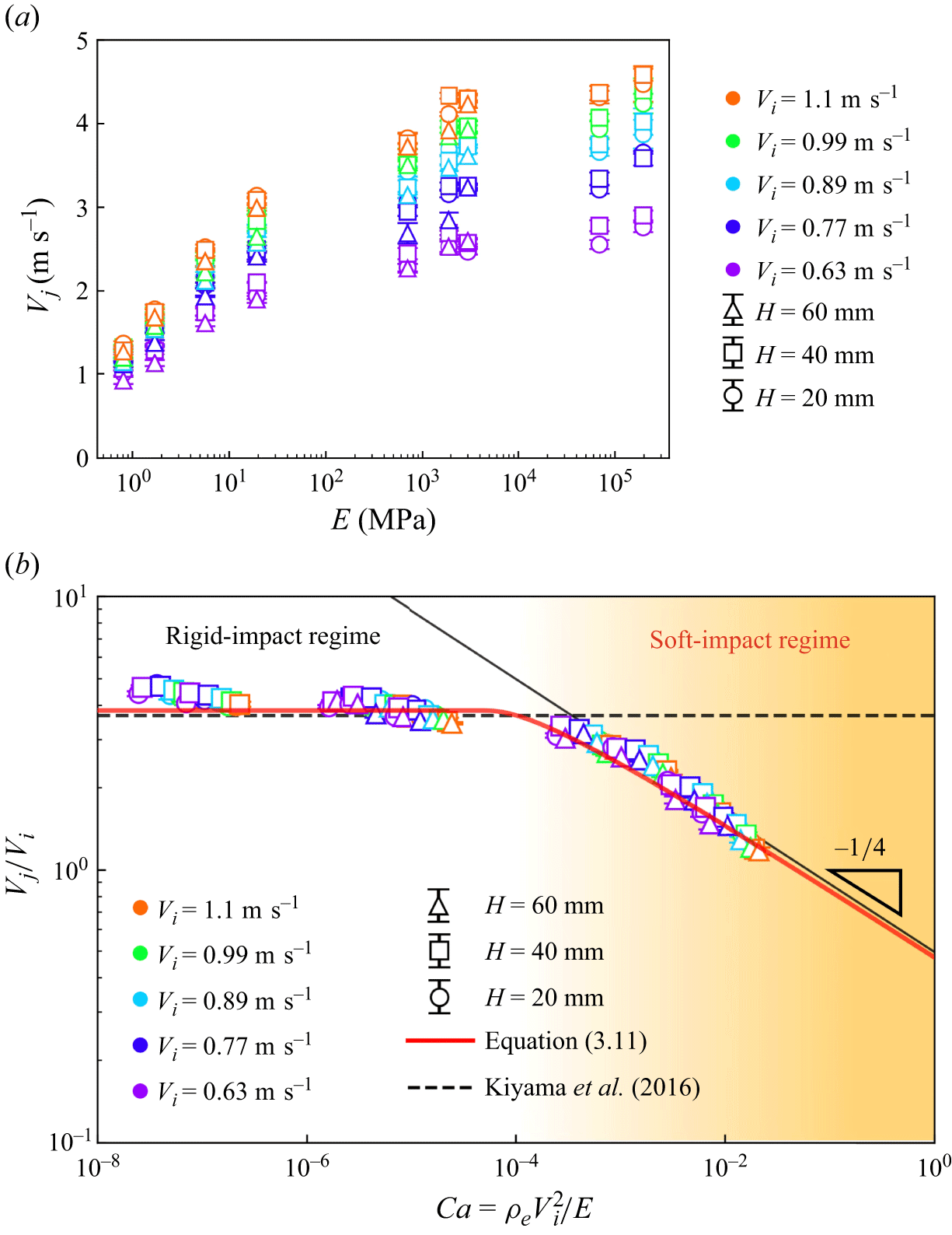
 Vj
 E
 Vj
 E
 Vi
 Vi
 E
 Vj
 E
 Vi
 Vj/Vi
 ρeVi2/E
 ρeVi2/E<10−4
 Vj/Vi
 ρeVi2/E>10−4
 Vj/Vi
 Vj/Vi=3.66
 −1/4

 ▴
 E=2.0×10⁵
 E=1.7×100
 E=8.1×10⁻¹
 H=20
 Vi=0.63
 t=0
 E=2.0×10⁵
 τimpact=0.2
 τfocusing=1.9
 τimpact≪τfocusing
 E=1.7×100
 8.1×10⁻¹
 Hm

 t=0
 t=τfocusing
 V′
 t=τfocusing
 F
 F
 E
 H=20
 Vi=0.63
 I
 E≥7.0×10²
 I
 F
 E≤1.9×101
 I
 F

 Vj
 (Vj/Vi)
 (I)
 Vj/Vi
 I
 E=8.1×10⁻¹
 5.7×100
 7.0×10²
 E
 Vj
 I
 Vj
 E=7.0×10²
 I
 F
 I
 Vj
 E=8.1×10⁻¹
 5.7×100
 F
 t=Hm/Vj
 I
 F
 Vj
 I
 E=8.1×10⁻¹
 I
 Hm/Vj
 τimpact

 δ
 P
 h
 Rs

 δ
 δ≥200 μm
 E

 α
 Ca
 α
 +2.6%
 −8.9%
 α=1.91
 α

 F
 E=2.0×10⁵
 1.9×10³
 5.7×100
 8.1×10⁻¹
 H=20
 Vi=0.63


 τfocusing
 Hm/Vj
 τfocusing=Hm/Vj
 Hm/Vj
 τfocusing


 Open access

