2 GAM dispersion relation for thermal particles

The ideal MHD model predicts that the GAM dispersion relation is given by (Winsor et al. Reference Winsor, Johnson and Dawson1968)

(2.1)\begin{equation} \omega_{{\rm Gmhd}}^{2} =\frac{\gamma p}{\varrho R_0^{2}} \left (2 + \frac{1}{q^{2}} \right ), \end{equation}

where $p$ is the plasma pressure, $\varrho$ is the density, $R_0$ the major radius, $q$ the safety factor and $\gamma$ is the adiabatic index.

The fully MHD code NOVA (Cheng & Chance Reference Cheng and Chance1987) was used to correct the GAM dispersion relation for accurate description, based on the MHD equations:

(2.2)\begin{equation} \left. \begin{aligned} \varrho \omega^{2} \frac{| \boldsymbol{\nabla} \psi |^{2}}{B^{2}}\xi_S+\left( \boldsymbol{B} \boldsymbol{\cdot} \boldsymbol{\nabla} \right ) \frac{| \boldsymbol{\nabla} \psi |^{2}}{B^{2}}\left ( \boldsymbol{B} \boldsymbol{\cdot} \boldsymbol{\nabla} \right ) \xi_S + \gamma p \boldsymbol{\nabla} \boldsymbol{\cdot} \boldsymbol {\xi} = 0,\\ \left( \frac{ \gamma p }{B^{2}} + 1 \right ) \boldsymbol{\nabla} \boldsymbol{\cdot} \boldsymbol {\xi} + \frac{ \gamma p }{ \varrho \omega^{2} } \left ( \boldsymbol {B} \boldsymbol{\cdot} \boldsymbol{\nabla} \right ) \frac {\boldsymbol{B} \boldsymbol{\cdot} \boldsymbol{\nabla} }{B^{2}} \boldsymbol{\nabla} \boldsymbol{\cdot} \boldsymbol{\xi} + k_s \xi_S =0, \end{aligned} \right\} \end{equation}

where $\psi$ is the poloidal magnetic flux, $\xi _S \equiv \boldsymbol {\xi } \boldsymbol {\cdot } | \boldsymbol {B} \times \boldsymbol{\nabla} \psi | /|\boldsymbol{\nabla} \psi |^{2}$,$\boldsymbol {\xi }$ is the plasma displacement, $k_S \equiv 2 \boldsymbol {k} \boldsymbol {\cdot } | \boldsymbol {B} \times \boldsymbol{\nabla} \psi | / |\boldsymbol{\nabla} \psi |^{2}$, and $\boldsymbol {k}$ and $\boldsymbol {B}$ are the vector of magnetic curvature and field.

The frequencies computed by NOVA are similar to those predicted by (2.1), but modified by sideband corrections. No further corrections are included such as due to different electron and ion temperatures, plasma rotation or the effect of impurities. The adiabatic index $\gamma$ in MHD equals $5/3$, but it is a free parameter inside NOVA and can be modified as needed to accommodate other corrections. The NOVA code (Cheng et al. Reference Cheng, Chen and Chance1985; Cheng & Chance Reference Cheng and Chance1986), together with its kinetic extension NOVA-K (Gorelenkov et al. Reference Gorelenkov, Cheng and Fu1999), is largely used to study Alfvénic, low frequency acoustic Alfvén-acoustic branches (Gorelenkov et al. Reference Gorelenkov, Berk, Fredrickson and Sharapov2007) as well other types of modes (Cheng & Chance Reference Cheng and Chance1987).

However, in the kinetic formulation, the GAM dispersion relation is given by (Lebedev et al. Reference Lebedev, Yushmanov, Diamond, Novakovskii and Smolyakov1996)

(2.3)\begin{equation} \omega_{{\rm Gkin}}^{2} =\left ( \frac{7}{4}+\tau_e+\frac{23+4\tau_e (4+ \tau_ e ) }{2 q^{2} (7 + 4 \tau_e )} \right ) \frac {v_{Ti}^{2}}{R_0^{2}}, \end{equation}

where $\tau _e = T_e/T_i$ is the ratio between the electron and ion temperatures and $v_{Ti} = \sqrt {2 T_i/ m_i}$ is the thermal ion velocity.

To calculate the dispersion relation, we introduce an effective kinetic-adiabatic-index $\gamma _k$, intended to match the result from MHD in (2.1) to the kinetic result in (2.3), defined as

(2.4)\begin{equation} \gamma_k \equiv \omega_{{\rm Gkin}}^{2} \left[ \frac {p}{\varrho R_0^{2}} \left ( 2 + \frac {1}{q^{2}} \right ) \right ]^{{-}1}. \end{equation}

This $\gamma _k$ will replace the the ideal MHD value of $5/3$. In fact, the corrections are normally not too large for simulations with just thermal particles, but can be as small as 0.8 in the case where the pressure $p$ in (2.1) contains energetic ions pressure, as used in EGAM (Nazikian et al. Reference Nazikian, Fu, Austin, Berk, Budny, Gorelenkov, Heidbrink, Holcomb, Kramer and McKee2008).

3 Kinetic calculations for the local dispersion relation and eigenmode

Using quasitoroidal coordinates, $(r,\vartheta, \zeta )$, with high aspect ratio $(R \gg r)$, for small Larmor radius, the drift kinetic equation (Hazeltine Reference Hazeltine1973) for $N=0$, can be written as

(3.1)\begin{equation} \frac{\partial f_\alpha }{\partial t} + \frac{v_\parallel}{q R}\frac{\partial f_\alpha }{\partial \vartheta} + v_{dr \alpha}\frac{\partial f_\alpha }{\partial r} = e_\alpha \frac{\partial F_\alpha }{\partial E} \left( \frac{v_{{\parallel}}}{qR}\frac{\partial \phi }{\partial \theta}+ v_{dr \alpha}\frac{\partial \phi }{\partial r} \right ), \end{equation}

where $f_\alpha = f_\alpha (r,\vartheta, v_{\parallel, \perp }, t)$ and $F_\alpha = F_\alpha (r,\vartheta, v_{\parallel, \perp })$ is the perturbed and equilibrium distribution function for each particle species $\alpha$, $v_{\parallel, \perp }$ is the velocity parallel and perpendicular to the magnetic field, $E$ is the particle energy, $\phi = \phi (r,\vartheta, t)$ is the perturbed electrostatic potential, and $R$ is the major radius and the radial magnetic drift velocity is given by $v_{dr \alpha } =-{ \sin \vartheta ( v_\parallel ^{2}+v_\perp ^{2}/2 )}/{\omega _{c \alpha } R}$, where $\omega _{c \alpha }$ is the cyclotron frequency.

Taking into account the poloidal oscillations $M=0,\pm 1, \pm 2$, and assuming the radial variation of the radial wave vector to be small, the perturbed functions can be expanded as

(3.2)\begin{equation} X (r,\vartheta, t) = \left [ X_0 + X_s \sin \vartheta + X_c\cos \vartheta + X_{2s} \sin 2 \vartheta + X_{2c} \cos 2 \vartheta \right ] \exp \left [{\rm i} k_r r - {\rm i} \omega t \right ]. \end{equation}

The Maxwellian distribution for thermal ions and electrons is

(3.3)\begin{equation} F_{i,e}=\frac{n_{0 i,e}}{{\rm \pi}^{3/2} v_{T i,e}^{3}} \exp [-(v_\parallel^{2}+v_\perp^{2})/v_{T i,e}^{2} ], \end{equation}

where $n_{0 i,e}$ is the equilibrium density for ions and electrons, $v_{T i,e}=\sqrt {2 T_{i,e} / m_{i,e}}$ is the thermal velocity, and $T_{i,e}$ and $m_{i,e}$ are the particle temperature and mass.

For the energetic particles (EP, beam ions in this case), the approximate slowing-down (Stix Reference Stix1972) function, valid for the injection beam velocity much larger than the critical velocity $(V_b \gg V_c)$ and the angular parameter $\lambda =v_\perp ^{2}/v^{2}$ with Gaussian distribution $\Delta \lambda _0 \ll 1$, is

(3.4)\begin{equation} F_{{\rm ep}} = \frac{n_{0{\rm ep}}\sqrt{1-\lambda_0}}{ {\rm \pi}^{3/2} \log[V_b/V_c] \Delta \lambda_0} \frac{ \exp [ - (\lambda-\lambda_0)^{2}/\Delta \lambda_0^{2} ]}{ v^{3}} . \end{equation}

To obtain the dispersion relation and calculate the eigenmode radial structure for $\phi _0$ (details in Appendix A), (3.1) is solved for electron, thermal and energetic ions. The density is calculated integrating $f_{s,c,2s,2c}$ over the velocity space to calculate $\phi _{s,c,2s,2c}$ via quasineutrality condition. The $\vartheta$-averaged radial current $\langle j_\alpha \rangle$ is calculated. From the neutrality condition for the radial current, we have $\sum _\alpha \langle j_\alpha \rangle + j_p = 0$, where the thermal ion polarization current is $j_p= -\textrm {i}\omega (1 - 3 \rho _{\textrm {th}}^{2} k_r^{2} /8 ) [ e_i^{2} n_{0i} / m_i \omega _{ci} ] d \phi _0/dr$. From the resonance condition, in the limit $\rho _\alpha ^{2}k_r^{2} \ll 1$, keeping terms up to $\rho _\alpha ^{2} k_r^{2}$, we obtain the dispersion relation (details in Appendix A):

(3.5)\begin{equation} [(D_{{\rm th}} +D_{{\rm ep}} )-(L_{{\rm th}} \rho_{{\rm th}}^{2}+L_{{\rm ep}} \rho_{{\rm ep}}^{2})k_r^{2}]k_r\phi_0 = 0, \end{equation}

where $\rho _{\textrm {th}}=v_{Ti}/\omega _{ci}$ and $\rho _{\textrm {ep}}=q V_b/\omega _{ci}$ are the Larmor radius for thermal and energetic ions, respectively, and the terms $D_{\textrm {th},\textrm {ep}}$ and $L_{\textrm {th},\textrm {ep}}$ correspond to the contributions to the dispersion relation and to FLR effects from thermal (th) and energetic particles (ep), given by (3.6)–(3.9) in the following.

The contribution to the dispersion relation due to the thermal particles is

(3.6)\begin{align} D_{{\rm th}}& = 1 - \frac{7+4\tau_e}{4}\frac{v_{Ti}^{2} \sigma_s^{2}}{R_0^{2} \omega^{2}} - \frac{23+16\tau_e+4\tau_e^{2} }{8 q^{2}} \frac{v_{Ti}^{4} \sigma_s^{4}}{R_0^{4} \omega^{4}},\nonumber\\ & \quad+{\rm i} q^{2} 2 \sqrt{ {\rm \pi}} \left [ \frac{\omega^{3} R_0^{3} q^{3}}{v_{Ti}^{3}} + (1+\tau_e) \frac{\omega R_0 q}{v_{Ti}} \right ] \exp{\left ( -\frac{\omega^{2} R_0^{2} q^{2}}{v_{Ti}^{2}} \right )}, \end{align}

where $\sigma _s \equiv \omega _{N} / \omega _{\textrm {Gkin}}$ is formally included, making the dispersion relation consistent with the one calculated by NOVA, $\omega _{N}$, which includes the sideband corrections, similar to a previous publication (Nazikian et al. Reference Nazikian, Fu, Austin, Berk, Budny, Gorelenkov, Heidbrink, Holcomb, Kramer and McKee2008), in the limit $v_{Ti} \ll \omega R_0 q \ll v_{\textrm {Te}}$.

The finite Larmor radius effect for thermal particles $L_{\textrm {th}}$ is given by

(3.7)\begin{equation} L_{{\rm th}}= \frac{3}{8}+ \frac{747+481\tau_e+140\tau_e^{2}+16\tau_e^{3}}{32} \frac{ v_{Ti}^{4} }{\omega^{4} R_0^{4}} . \end{equation}

In the limit $\Delta \lambda _0 \ll 1$, the influence of EP in the local dispersion relation is given by

(3.8)\begin{align} D_{{\rm ep}}& = C_D \left [ \frac{2 \lambda_0 \left ( 2-\lambda_0 \right )^{2} \omega_{{\rm tr}}^{2}}{\left ( \omega_{{\rm tr}}^{2}-\omega^{2} \right )} -\Delta \lambda_0^{2} \frac{3 \left ( 2-\lambda_0 \right ) \left( 4 \omega_ {tr}^{2} - \omega^{2}(2+\lambda_0) \right )\omega_{{\rm tr}}^{2}}{ 4 \left ( 1-\lambda_ 0 \right )\left ( \omega_{{\rm tr}}^{2} - \omega^{2} \right )^{2}} \right .\nonumber\\ & \quad \left . -\left ( \left( 5\lambda_0 - 2 \right ) \left ( 2-\lambda_0 \right ) - \frac {15 \Delta \lambda_0 ^{2} }{4 \left ( 1-\lambda_0 \right ) } \right ) \log \left ( 1 - \frac{\omega_{{\rm tr}}^{2}}{\omega^{2}} \right ) \vphantom{\frac{2 \lambda_0 \left ( 2-\lambda_0 \right )^{2} \omega_{{\rm tr}}^{2}}{\left ( \omega_{{\rm tr}}^{2}-\omega^{2} \right )}}\right ], \end{align}

where $C_D= {n_{0\textrm {ep}} }/n_{0i} {16 (1-\lambda _0)^{2} \log [ V_b/V_c ]}$ and $\omega _{\textrm {tr}} = V_b \sqrt {1-\lambda _0}/q R_0$ is the transit frequency for EP injection velocity.

The EP FLR effect contribution is given by

(3.9)\begin{align} L_{{\rm ep}}& = C_L \left \{ -\frac{3 \left (\left ( 20 \lambda_0- 8 + 8 \lambda_0^{2} \right )\omega_{{\rm tr}}^{4} - 5 \omega_{{\rm tr}}^{2} \omega^{2} (9 \lambda_0 - 2)\right )}{4 \left ( 4 \omega_{{\rm tr}}^{2}-\omega^{2} \right )\left ( \omega_{{\rm tr}}^{2}-\omega^{2} \right )} \right .\nonumber\\ & \quad -\Delta \lambda_0^{2} \frac{16(600 \omega_{{\rm tr}}^{6} \omega^{2} - 611 \omega_{{\rm tr}}^{4} \omega^{4} - 112 \omega_{{\rm tr}}^{8} + 190 \omega_{{\rm tr}}^{2} \omega^{6} )}{64 (4 \omega_{{\rm tr}}^{2} - \omega^{2})^{2} ( \omega_{{\rm tr}}^{2} - \omega^{2} )^{2} (2 - \lambda_0)} \nonumber\\ & \quad \left .+\left ( \left ( 9\lambda_0-2 \right ) - \Delta \lambda_0 ^{2} \frac {57}{4 \left ( 1-\lambda_0 \right )\left ( 2-\lambda_0 \right ) } \right ) \left [ \frac{\omega^{2}}{\omega_{{\rm tr}}^{2}} \log \left ( 1 - \frac{\omega_{{\rm tr}}^{2}}{\omega^{2}} \right ) -\frac{\omega^{2}}{16 \omega_{{\rm tr}}^{2}}\log \left ( 1 - 4\frac{\omega_{{\rm tr}}^{2}}{\omega^{2}} \right ) \right ] \vphantom{\frac{3 \left (\left ( 20 \lambda_0- 8 + 8 \lambda_0^{2} \right )\omega_{{\rm tr}}^{4} - 5 \omega_{{\rm tr}}^{2} \omega^{2} (9 \lambda_0 - 2)\right )}{4 \left ( 4 \omega_{{\rm tr}}^{2}-\omega^{2} \right )\left ( \omega_{{\rm tr}}^{2}-\omega^{2} \right )}}\right \}, \end{align}

with $C_L = (({(2- \lambda _0)^{3}})/({16 (1-\lambda _0)})) C_D$.

For only the thermal GAM dispersion relation, $D_{\textrm {th}}=0$. Disregarding NOVA side-band corrections and Landau damping from the imaginary part, its solution recovers the frequency given by (2.3). The EGAM dispersion relation is found for $D_{\textrm {th}} +D_{\textrm {ep}} =0$. It follows from (3.8) that the contribution from EP to the dispersion relation rises as $\omega _{\textrm {tr}}$ approaches $\omega$, and the instability is found only for the solution with ${\omega _{\textrm {tr}}}>{\omega }$. This result is similar to that obtained previously (Qiu et al. Reference Qiu, Zonca and Chen2010), with additional terms giving a small contribution from the Gaussian angular parameter $\Delta \lambda _0$.

From the imaginary part of the dispersion relation, the linear growth rate $\gamma _G$ can be calculated as $\omega = \omega _G+\textrm {i} \gamma _G$, with $\gamma _G \ll \omega _G$, leading to

(3.10)\begin{align} \gamma_G & \approx \omega_G^{2} q^{2} \sqrt{\rm \pi} \left \{ \sqrt{\rm \pi} C_D \left [ \left( 5\lambda_0 - 2 \right ) \left ( 2-\lambda_0 \right ) - \frac {15 \Delta \lambda_0 ^{2} }{4 \left ( 1-\lambda_0 \right ) } \right ] \right .\nonumber\\ & \quad \left. - \frac{ R_0 q}{v_{Ti}} \left [ \frac{\omega_G^{2} R_0^{2} q^{2}}{v_{Ti}^{2}} + (1+\tau_e) \right ] \exp{\left ( - \frac{\omega_G^{2} R_0^{2} q^{2}}{v_{Ti}^{2}} \right )}\right \}, \end{align}

where the first term represents the drive given by the EP, which decreases with larger $\Delta \lambda _0$, similar to numerical calculation (Chen et al. Reference Chen, Zhang, Bao, Lin, Dong, Cao and Li2020) for $\Delta \lambda _0 < 0.2$, while the second term represents the thermal ion Landau damping. It follows from (3.10) that a necessary condition for instability ($\gamma _G >0$) is $\lambda _0 > 0.4$ for $\Delta \lambda _0=0$ and it increases up to $\lambda _0 > 0.43$ for $\Delta \lambda _0=0.2$, where the additional contribution from the energetic particles easily overcome the Landal damping from thermal ions.

Finally, we can obtain the eigenmode equation, using the approximation $\partial /\partial r \sim \textrm {i} k_r$, going back to the derivative form, we can rewrite (3.5) as a differential equation for the radial electric field $E_r(r,\omega ) = -({\partial \phi _0}/{\partial r})$ as

(3.11)\begin{equation} Q(r,\omega) \frac{\partial \phi_0}{\partial r}+\frac{\partial^{2}}{\partial r ^{2}} \frac{\partial \phi_0}{\partial r}=0, \end{equation}

where $Q(r,\omega )={ (D_{\textrm {th}} +D_{\textrm {ep}} )}/{(L_{\textrm {th}} \rho _{\textrm {th}}^{2}+L_{\textrm {ep}} \rho _{\textrm {ep}}^{2})}$.

In the complete differential equation, the FLR effect will ‘decouple’ the eigenmode from the dispersion relation; in this case, the radial distribution for the electrostatic potential $\phi _0$ can be found.

The solution for the eigenmode is obtained integrating numerically (3.11), setting $\omega$ very close to the maximum of dispersion relation, in the vicinity of the turning points ($r \sim 0$) and around $Q \sim 0$. Far from this point, the numerical solution is matched with the WKB approximation:

(3.12)\begin{equation} \frac{{\rm d} \phi_0}{{\rm d}r} = \frac{C_1 \exp({{\rm i} \int \sqrt{Q}\,{\rm d}r}) + C_2 \exp({-{\rm i} \int \sqrt{Q} \,{\rm d}r})}{Q^{1/4}}. \end{equation}

It is important to point out that, in some cases, numerical physical solutions will appear only for rather specific initial conditions, i.e. those that will be matched by the WKB approximation with $C_2 = 0$, to avoid the exponential growth due to $\mathrm {Im} (\sqrt {Q})$ in the second term of the right-hand side of (3.12). However, to proceed with the numerical calculation of the eigenfunction, as each step will introduce errors by numerical truncation, it is necessary to disregard the imaginary part of the FLR effect, $\mathrm {Im} (L_{\textrm {th},\textrm {ep}})$, to avoid runaway problems in the numerical convergence due to the stiffness of the eigenvalue equation (LeVeque Reference LeVeque2007).

A physical solution is found by solving (3.11) for $\omega$ for a value very close to the maximum of dispersion relation, where $Q \sim 0$. When that maximum is located at the axis, the radial distribution is strongly oscillatory, due to monotonic increase of $Q$. However, when the EP contribution in the dispersion relation is strong enough to produce a off-axis maximum, as predicted in previous works on global EGAM (Qu et al. Reference Qu, Hole and Fitzgerald2017), we will see the eigenmode located around the maximum of the dispersion relation, and due to the model used here, an outgoing wave (Qiu et al. Reference Qiu, Zonca and Chen2010) given by $C_1 \exp ({\textrm {i} \int \sqrt {Q} \,\textrm {d}r})/Q^{1/4}$.

4 Comparison to experimental DIII-D $N=0$ oscillation

The results of this work are applied to model EGAM oscillations in DIII-D during discharge ramp-up. The discharge #159243 (Collins et al. Reference Collins, Heidbrink, Austin, Kramer, Pace, Petty, Stagner, Van Zeeland, White and Zhu2016; Heidbrink et al. Reference Heidbrink, Collins, Podesta, Kramer, Pace, Petty, Stagner, Van Zeeland, White and Zhu2017; Gorelenkov et al. Reference Gorelenkov, Duarte, Podesta and Berk2018) was chosen due to the presence of sweeping up RSAE, where their frequency lies in between the GAM and TAE frequencies, and also indicates the evolution of the reverse $q$ profile.

In the simulations, we use the profiles of $q$ and temperature presented in figure 1(a) and of density, given by TRANSP, and calculated effective $\gamma _k$, given by (2.4), presented in figure 1(b).

Figure 1.

(a) Profiles of $q$, ion (black) and electron (red) temperature, at 500 ms (solid) and 900 ms (dashed). (b) Profiles of thermal ion densities (deuterium and carbon), EP (deuterium) and the effective $\gamma _k$.

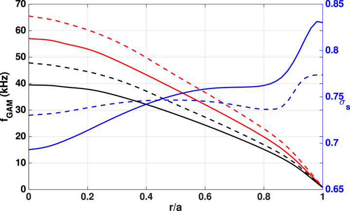
The dispersion relation is accurately calculated using NOVA and presented in figure 2, showing the side-band corrections $\sigma _s \approx 0.68\unicode{x2013}0.75$ in the region where the EP transit frequency is close to the thermal GAM frequency.

Figure 2.

Dispersion relation calculated purely kinetically ($\omega _{\textrm {Gkin}}$, red) and corrected by NOVA (black), with respective $\sigma _s$ in blue, for 500 ms (solid) and 900 ms (dashed).

The discharge #159243 (Collins et al. Reference Collins, Heidbrink, Austin, Kramer, Pace, Petty, Stagner, Van Zeeland, White and Zhu2016; Heidbrink et al. Reference Heidbrink, Collins, Podesta, Kramer, Pace, Petty, Stagner, Van Zeeland, White and Zhu2017; Gorelenkov et al. Reference Gorelenkov, Duarte, Podesta and Berk2018) has multiple beam injections, mostly from co-tangential sources, with the main injection energy from 70 to 80 keV, and a minor density with half of the injected particles with injection with energy lower than 40 keV; however, only the higher energies are included in the simulations. There is also a minor density from the counter-tangential source not modelled. Furthermore, the injection angle $\lambda _0$ changes for different energies of the particles, as can be seen in figure 4 of Gorelenkov et al. (Reference Gorelenkov, Duarte, Podesta and Berk2018), where around the injection energy (70–80 keV), it is found that $\lambda _0 \sim 0.6$ is decreasing for smaller energies, towards parallel motion.

In the theoretical model, there is a single $\lambda _0$ and single injection energy. In the simulations, while small variations in the injection energy in the range of 70–80 keV have a minor impact on the final result, the $\lambda _0$ value substantially influences the dispersion relation. To account for this variability in the simplified theoretical model, the calculations are carried out at a range of $\lambda _0$ values, and the results are represented as ‘error bars’ in the calculated spectrum of oscillations; this is shown in figure 4 for $0.5<\lambda _0<0.6$. A single injection energy of 75 keV is used.

The respective dispersion relation is presented in figure 3(a) before (500 ms) and in figure 3(b) after (900 ms) the marginal stability point. In the calculations, the ratio between the electron and ion temperatures is taken as $\tau _e \sim 0.86$.

Figure 3.

Dispersion relation for 500 and 900 ms, the thermal GAM simulated by NOVA (blue), the EP transit frequency (green), local dispersion relation (red) and maximum of local dispersion relation (black), the maxima are found at $r/a=0.3$, $f=28$ kHz in panel (a) and $r/a=0$, $f=39$ kHz in panel (b). (a) 500 ms. (b) 900 ms.

In simulations leading to the results shown in figure 4, we use $n_{0\textrm {ep}} \sim 0.04 n_{0i}$ in the time interval from 500 ms–700 ms, as the effect is dominated by $\lambda _0$ and $q$. In the time interval from 700 ms to 900 ms, i.e. around the marginal stability point, a small radial variation of $n_{0\textrm {ep}}$ may be useful to find the exact marginal stability point. We use $n_{0\textrm {ep}} \sim 0.04\unicode{x2013}0.08 n_{0i}$ as in figure 1(b), calculated by the kick model profile (Podesta, Gorelenkova & White Reference Podesta, Gorelenkova and White2014; Podesta et al. Reference Podesta, Gorelenkova, Gorelenkov and White2017), which has good agreement with FIDA measurements of co-passing EP (Collins et al. Reference Collins, Heidbrink, Austin, Kramer, Pace, Petty, Stagner, Van Zeeland, White and Zhu2016; Heidbrink et al. Reference Heidbrink, Collins, Podesta, Kramer, Pace, Petty, Stagner, Van Zeeland, White and Zhu2017).

Figure 4.

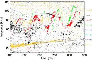
Mirnov coils oscillations from shot #159243 showing RSAE between $40\textrm { and }100$ kHz and $N=0$ mode (yellow) starting from $25\unicode{x2013}30$ kHz at 500 ms and disappearing at approximately $35\unicode{x2013}40$ kHz close to 800 ms. The grey line represents the time evolution of the calculated frequency for the maximum of the dispersion relation. The error bars are due to simulation for $0.5 < \lambda _0 < 0.6$, and the X means that the maximum is found on axis.

An $N=0$ oscillation with growing frequency starting from $25\unicode{x2013}30$ kHz at 500 ms and disappearing at approximately $35\unicode{x2013}40$ kHz around 800 ms, captured by Mirnov coils as magnetic oscillation at the edge of plasma column, are presented in yellow in figure 4, below the sweeping up RSAE, $40\unicode{x2013}100$ kHz and $N > 1$. The grey line shows the result of the simulated frequency of the maximum of the dispersion relation, matching the observed $N=0$ oscillation inside the error bars. The error bars represent two extremes of the frequency calculated using injection angle as $\lambda _0=0.5$ for the higher limit, and $\lambda _0=0.6$ for the lower one. The X means that the maximum of the dispersion relation is found on axis, as in figure 3(b) for 900 ms, indicating that no eigenmode should be found, as showed in §§ 5 and 6, and the disappearance of the oscillation at some time between $750\textrm { and }850$ ms.

It is important to point that the temporal evolution of profiles does not affect the growth rate significantly enough to explain the dissipation of the oscillation close to 800 ms, in terms of the relation between the energetic ion driven oscillation and thermal ion Landau damping, $\gamma _G\sim 4 \unicode{x2013}10\,\%$ for the simulations above, allowing the conclusion that the stabilization is due to differences in the dispersion relation.

5 Maximum off axis – Radial profile for the EGAM oscillation

We choose the following analytic profiles for the thermal and energetic particles consistent with TRANSP profiles reconstruction. The profiles listed in this section were chosen based on the parameters for the DIII-D discharge at 500 ms, with deuterium and carbon as thermal ions, the $q$ profile as $q=4.7-10(r/a)^{2}+14.8(r/a)^{3}-2(r/a)^{4}$ for $q=4.7$ in the centre, $\textrm {d}q/\textrm {d}r|_{r=0} \sim 0$, $q_{\textrm {min}}=3.9$ at $r_{q\textrm {min}}=0.5$ and 7.4 at $r=a$, and the temperature of thermal ions as $T_i=[1.8(1-(r/a)^{2})^{2.5}+0.1]\,\textrm {keV}$. For the energetic ions profile, just calculating for the passing particles, the ratio of density between energetic ions and thermal ions is taken equal to $4\,\%$ for $0 < r/a < 0.45$, decreasing to 0 for $r/a > 0.45$. This new restriction is necessary to avoid including energetic ions near the edge, where the approximation $\rho _{\textrm {ep}}^{2} k_r^{2} <1$ may not be valid and the effects of trapped particles should be included in the theoretical formulation as they may not be negligible for $r/a > 0.45$. The injection energy is 70 keV and injection angle is $\lambda _0 = 0.5$, with angular distribution $\Delta \lambda _0=0.2$. Using the critical velocity as $V_c \sim 5.5 A_b^{1/3} \sqrt {T_e/ m_b}$ (Stix Reference Stix1972) and the MHD correction $\sigma _s \sim 0.7$ given by NOVA simulations, the maximum off axis appears clearly.

The dispersion relation is represented in figure 5, where $f=\omega /2 {\rm \pi}$.

Figure 5.

Dispersion relation for thermal particles in blue, EP transit frequency in green and the local dispersion relation in red. The maximum of the dispersion relation is found at $f_{\textrm {G-EGAM}}=28.1$ kHz at $r/a=0.32$ and the respective growth rate ${\gamma _G}/{\omega _G}=5.8\,\%$.

We can see that the coupling is stronger in the central plasma region, because of the reverse $q$ profile, which produces a maximum at approximately $r/a=0.27$ for $f=28.1$ kHz. The associated growth rate is 9.3 % of the mode frequency. The frequency calculated from the dispersion relation starts to drop significantly for $r/a>0.5$. To determine the eigenfunction, it is necessary to calculate the radial profile of the quantity $Q$, in (3.11). This is shown in figure 6(a) for the radial interval $0< r<0.5$ and for the frequency at the maximum of the dispersion relation. We note that the imaginary part of the FLR effect, $\mathrm {Im}(L_{\textrm {th},\textrm {ep}})$, is disregarded in this calculation to avoid runaway numerical solutions, for the reason already mentioned. For $r/a>0.5$, both the real and imaginary parts of $Q$ grow monotonically, with $\mathrm {Im}(Q) \ll \mathrm {Re}(Q)$, as $\rho _{\textrm {th}}$ decreases as the temperature decreases with $r$.

Figure 6.

(a) $\mathrm {Re}(Q)$ in black and $\mathrm {Im}(Q)$ in green, on the maximum of the dispersion relation, $f_{\textrm {G-EGAM}}=28.1$ kHz with the respective growth rate ${\gamma _G}/{\omega _G}=9.3\,\%$. (b) Solution for real (black) and imaginary (green) parts of the eigenmode, $\textrm {d}\phi _0 /\textrm {d}r$ (a.u.), showing the Airy function for $r/a<0.45$ and oscillatory for $r/a>0.45$.

The eigenfunction is numerically calculated in the interval $0< r/a<0.45$, where the solution for $\textrm {d}\phi _0/\textrm {d}r$ is given by the Airy function, and matches the respective WKB solution, (3.12), for $r/a>0.45$, where the solution becomes strongly oscillatory as $Q \rightarrow \infty$, ultimately vanishing at the edge, as shown in figure 6(b), representing how the radial structure of the EGAM eigenmode looks like when a off-axis maximum is present. The eigenmode in figure 6(b) is normalized by its first minimum as we will compare the global behaviour of the first maximum with respect to the pure radially oscillatory solution.

For higher ion temperatures at the edge, only some specific frequencies should result in $\textrm {d}\phi _0/\textrm {d}r=0$ as $r/a \rightarrow 1$. In any case, the solution is very similar to figure 6(b), with no substantial changes in the frequency and growth rate.

While the condition $\rho _{\textrm {th}}^{2} k_r^{2} \ll 1$ is always easily satisfied, it is not necessarily true for the energetic ions. The consistency of the approximation for energetic ions is checked and the condition $\rho _{\textrm {ep}}^{2} k_r^{2} \approx 0.6$ is verified. The result found for the eigenfunction is similar to previous calculations for GAM in MHD, numerically (Berk et al. Reference Berk, Boswell, Borba, Figueiredo, Johnson, Nave, Pinches and Sharapov2006) and analytically (Lakhin & Sorokina Reference Lakhin and Sorokina2014), showing strong coupling to the dispersion relation near its maximum. In our case, instead of a Dirac function for $\textrm {d}\phi _0/\textrm {d}r$, the solution is spatially distributed. It is also very similar to kinetic numerical results for EGAM (Fu Reference Fu2008; Qu et al. Reference Qu, Hole and Fitzgerald2017), especially in the region around the centre. The $M=\pm 1,\pm 2$ poloidal components of perturbed electrostatic potential of the EGAM can be found using a similar method, following (A30)–(A31) in Appendix A.

It is important to note that EGAM branch oscillatory behaviour in the absence of EPs, i.e. when $r/a>0.45$, is obtained in the approximation $\rho _\alpha ^{2} k_r^{2} \ll 1$, leading to the eigenmode differential equation (3.11). Equation (3.11) is similar to equations previously published for EGAM (Qiu et al. Reference Qiu, Zonca and Chen2010) and thermal GAM (Itoh et al. Reference Itoh, Itoh, Sasaki, Fujisawa, Ido and Nagashima2007), when those modes are excited near the plasma edge. It is expected that including ions with the Larmor radius of the same order or larger than the radial wavelength, such as including EP Larmor radius at $r/a>0.45$ in our case, would average out the radial oscillation and reduce the amplitude of (E)GAMs, and would be closer to numerical calculations (Fu Reference Fu2008).

6 Maximum on axis – Radial profile for the EGAM oscillation

Now we consider the profiles similar to TRANSP reconstruction for t=900 ms, namely, the $q$ profile as $q=3-1.8(r/a) -4(r/a)^{2}+9.6(r/a)^{4}$ for $q=3$ in the centre, $\textrm {d}q/\textrm {d}r|_{r=0} \sim 0$, $q_{\textrm {min}}=2.65$ at $r_{q\textrm {min}}=0.5$ and 6.8 at $r=a$, the temperature of thermal ions as $T_i=[2(1-r^{2})^{2.5}+0.1]\,\textrm {keV}$, and the same energetic ions profile as used earlier in § 5; for EP, we take $n_{0\textrm {ep}} = 0.04 n_{0i}$ for $0 < r < 0.4$ to avoid including energetic ions near the edge, where the approximation $\rho _{\textrm {ep}}^{2} k_r^{2} <1$ breaks down. The solutions of the dispersion are represented in figure 7.

Figure 7.

Dispersion relation for thermal particles in blue, EP transit frequency in green and the local dispersion relation in red. The maximum of the dispersion relation is found at $f_{\textrm {G-EGAM}}=39.2$ kHz at $r/a=0$ and the respective growth rate ${\gamma _G}/{\omega _G}=7.9\,\%$.

We see that the coupling is not strong enough to produce an off-axis maximum, and the local frequency decreases monotonically, making $Q$ monotonically increase. This quantity is calculated as described in § 3.

In this case, the eigenfunction is numerically calculated in the interval $0< r/a<0.3$ and matched to the WKB solution for $r/a>0.3$. Using the same criterion from figure 6(b), the eigenmode in figure 8(b) is also normalized by its first minimum. The first maximum is the important part for the total increase of electrostatic potential and is much less pronounced in the on-axis case. It is clear that now the eigenfunction loses somewhat the global behaviour shown in the previous case, becoming radially oscillatory over the entire radial interval, in other terms, the eigenfunction of the on-axis case, for $r/a > 0$ is equivalent to the eigenfunction of the off-axis case, for $r/a > 0.32$. Due to the small variation of the dispersion relation as $r/a \rightarrow 0$, in the on-axis case, the eigenfunction presents a vestige of global behaviour as in figure 8(b), but this is negligible near the robust global behaviour of figure 6(b). The approximation of small Larmor radius remained valid in these calculations, i.e. $\rho _{\textrm {ep}}^{2} k_r^{2} \approx 0.6$.

Figure 8.

(a) $\mathrm {Re}(Q)$ in black and $\mathrm {Im}(Q)$ in green, on the maximum of the dispersion relation, $f_{\textrm {G-EGAM}}=39.2$ kHz with the respective growth rate ${\gamma _G}/{\omega _G}=7.9\,\%$. (b) Solution for real (black) and imaginary (green) parts of the eigenmode, $\textrm {d}\phi _0 / \textrm {d}r$ (a.u.) for the on axis maximum case.

The solution is also similar to the kinetic numerical results for EGAM (Qu et al. Reference Qu, Hole and Fitzgerald2017) for the monotonically increasing $q$, which does not produce an off-axis maximum either.