


1. Introduction
Inertia-dominated, wall-sheared turbulent flows are vertically composed of an inner layer and an inertial (outer) layer. Instantaneously, the former is occupied by sinuous streaks evolving in an autonomous inner cycle while the latter is composed of coherent,  $\delta$-scale regions of momentum excess and deficit, where
 $\delta$ is the flow depth (Townsend Reference Townsend1951; Kline et al. Reference Kline, Reynolds, Schraub and Rundstadler1967; Jimenez & Pinelli Reference Jimenez and Pinelli1999; Adrian, Meinhart & Tomkins Reference Adrian, Meinhart and Tomkins2000; Schoppa & Hussain Reference Schoppa and Hussain2002; Adrian Reference Adrian2007; Hutchins & Marusic Reference Hutchins and Marusic2007). The emergence of outer-layer dynamics is known to correlate with attainment of sufficient inertial conditions, commonly defined via friction Reynolds number,
 $Re_\tau = u_\tau \delta / \nu$, where
 $u_\tau$ is shear velocity and
 $\nu$ is kinematic viscosity. For canonical wall-sheared turbulence, contours of spectral density plotted against wall-normal position and constituent streamwise wavelength,
 $\lambda _1/\delta$, are known to exhibit a corresponding inner and outer peak. The inner peak embodies relatively greater energetic content, owing to intense production of turbulence within the inner layer. Energetic content within the outer peak physically represents energy-containing very-large-scale motions (Kim & Adrian Reference Kim and Adrian1999; Guala, Hommema & Adrian Reference Guala, Hommema and Adrian2006; Balakumar & Adrian Reference Balakumar and Adrian2007; Hutchins & Marusic Reference Hutchins and Marusic2007; Marusic & Hutchins Reference Marusic and Hutchins2008), which are generally viewed as the product of a streamwise coalescence of ‘building block’ large-scale motions (LSMs).
For asymptotic inertial conditions – common in a range of practically important engineering and geophysical flows – the inner cycle is ablated. The ‘lower region’ is subsequently occupied by a roughness sublayer (Raupach, Antonia & Rajagopalan Reference Raupach, Antonia and Rajagopalan1991; Jimenez Reference Jimenez2004) with wall-normal thickness scaling linearly with some representative measure of roughness amplitude,  $h$. For adequately small values of
 $h$,
 $\delta /h \gtrsim 20$ (Flack, Schultz & Connelly Reference Flack, Schultz and Connelly2007; Wu & Christensen Reference Wu and Christensen2007), vortical processes within the roughness sublayer are generally presumed to homogenize due to ambient shear, such that an outer peak in spectral density is able to develop (Townsend Reference Townsend1951).
For such inertia-dominated conditions, Reynolds-averaged (equilibrium) streamwise velocity and its associated wall-normal gradient exhibit a corresponding vertical dependence:
 \begin{equation} \frac{\langle u_1 \rangle_{12t} (x_3)}{u_\tau} = \frac{1}{\kappa} \log \left(\frac{x_3}{\ell}\right) \quad \textrm{and}\quad \frac{\textrm{d} \langle u_1 \rangle_{12t} (x_3)}{\textrm{d}\kern 0.06em x_3} = \left(\frac{u_\tau}{\kappa x_3}\right), \end{equation}
where  $\kappa$ is the von Kármán constant (Pope Reference Pope2000) and
 $\ell$ is a roughness length, physically equivalent to the elevation at which
 ${\langle u_1 \rangle _{12t} (x_3)}{u_\tau } = 0$; in this article, the first, second and third component of any vector corresponds to its magnitude in the streamwise, spanwise and wall-normal directions, respectively, while averaging over dimension
 $a$ is denoted by
 $\langle \cdots \rangle _a$, where subscript
 $t$ denotes Reynolds averaging.
Large-scale, nonlinear deviation from Reynolds-averaged conditions is inherent to wall-sheared turbulence. Nevertheless, these flows are known to exhibit a range of periodic attributes (structural and/or dynamical), from the emergence of vortical hairpin packets (Adrian et al. Reference Adrian, Meinhart and Tomkins2000; Ganapathisubramani, Longmire & Marusic Reference Ganapathisubramani, Longmire and Marusic2003; Adrian Reference Adrian2007), spatial attributes of LSMs (Hutchins & Marusic Reference Hutchins and Marusic2007) and correlation between space–time dynamics of inner- and outer-layer structure (Mathis, Hutchins & Marusic Reference Mathis, Hutchins and Marusic2009; Marusic, Mathis & Hutchins Reference Marusic, Mathis and Hutchins2010). This survey, though hardly exhaustive, illustrates the breadth of efforts devoted to recognition of patterns underpinning the dynamics of wall-sheared turbulence. With this, we are concerned here with the topic of uniform momentum zones (UMZs; Meinhart & Adrian Reference Meinhart and Adrian1995), an area of significant recent interest in the community (Priyadarshana et al. Reference Priyadarshana, Klewicki, Treat and Foss2007; de Silva et al. Reference de Silva, Philip, Hutchins and Marusic2017; Bautista et al. Reference Bautista, Ebadi, White, Chini and Klewicki2019; Fan et al. Reference Fan, Xu, Yao and Hickey2019; Heisel et al. Reference Heisel, de Silva, Hutchins, Marusic and Guala2020; Montemuro et al. Reference Montemuro, White, Klewicki and Chini2020; Heisel et al. Reference Heisel, de Silva, Hutchins, Marusic and Guala2021).
Uniform momentum zones manifest as inclined zones of relative momentum excess or deficit around the Reynolds-averaged structure. Instantaneously, this results in an ostensible staircase-like pattern in streamwise velocity. The interfacial region between inclined UMZs is occupied by elevated shear. de Silva et al. (Reference de Silva, Philip, Hutchins and Marusic2017) used experimental data to illustrate underlying self-similarity in shear intensity across UMZ interfaces, also termed vortical fissures (Bautista et al. Reference Bautista, Ebadi, White, Chini and Klewicki2019). More recently, Montemuro et al. (Reference Montemuro, White, Klewicki and Chini2020) presented evidence that a self-sustaining mechanism was responsible for dynamic and spatial attributes of UMZs. These results are consistent with contributions from Heisel et al. (Reference Heisel, de Silva, Hutchins, Marusic and Guala2021), who interpreted vortical flow processes between successive UMZs via ‘prograde’ vortices, and showed that vorticity thickness scales linearly with Taylor microscale,  $\lambda _T$, as expected (Morishita, Ishihara & Kaneda Reference Morishita, Ishihara and Kaneda2019).
In recent complementary work, Anderson & Salesky (Reference Anderson and Salesky2021) leveraged access to results from direct numerical simulation (DNS) at  $Re_\tau = 182$, 544, 1000, 1995 and 5185 (Lee & Moser Reference Lee and Moser2015). The data provided a unique opportunity to simultaneously assess inner- and outer-layer dynamics under inertia-dominated conditions. Anderson & Salesky (Reference Anderson and Salesky2021) demonstrated that the presence of UMZs in the outer layer originates via antecedent dynamics within the inner layer. It was beyond the scope of Anderson & Salesky (Reference Anderson and Salesky2021) to establish causality or dynamical hierarchy.
Anderson & Salesky (Reference Anderson and Salesky2021) used instantaneous  $x_1 - x_3$ spatial transects of fluctuating streamwise velocity to highlight how abrupt interactions within the inner layer set the origin for outer-layer UMZs. These inner-layer collisions and outer-layer UMZs were interpreted as bluff-body-like interactions and resultant wakes, respectively. Viewed in this framework, Anderson & Salesky (Reference Anderson and Salesky2021) show that instead of the ambient shear owing to the balance of momentum – establishing a Reynolds-averaged state leading to recovery of equilibrium conditions leading to (1.1a,b) – the ‘staircase-like’ flow structure necessitates a corresponding shear profile resembling a pulse signal with amplitude scaling as
 $\partial _3 u_1 ({\boldsymbol x}_l,x_3,t) \sim x_3^{-1/2}$, where
 ${\boldsymbol x}_l$ denotes an arbitrary discrete streamwise–spanwise location. This dependence exceeds logarithmic scaling by
 $x_3^{1/2}$ (equation (1.1a,b)), indicating the relatively larger shear exhibited across the interfacial regions between successive UMZs.
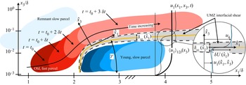
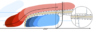
These results can be appreciated from figure 1, which depicts the inner-layer collision of a relatively older momentum excess (red) and relatively younger momentum deficit (blue). We highlight the envisioned time evolution of these structures, where the younger parcel acts as a bluff obstacle such that the older parcel evolves in a wake-like pattern; idealized stages of this interaction process are depicted at four instants. The interfacial region is used to set the origin of a local coordinate system,  $\widehat {\boldsymbol x}$, which is inclined at angle
 $\gamma$, the inclination angle commonly recorded for these structures (Marusic & Heuer Reference Marusic and Heuer2007). This resulting interfacial shear exhibits vorticity thickness,
 $\delta _\omega (\hat {x}_1)$, and increment,
 $\delta U(\hat {x}_1)$ (discussion of additional figure 1 attributes to follow). By posing the figure 1 interaction and resultant outer-layer structure as a turbulent wake, Anderson & Salesky (Reference Anderson and Salesky2021) were able to leverage existing scaling arguments for the channel turbulence context (Tennekes & Lumley Reference Tennekes and Lumley1972). It is worthwhile to question the description of these processes as being the product of inclined shear layers – as depicted in figure 1 and proposed in prior work (Klewicki Reference Klewicki2013a,Reference Klewickib,Reference Klewickic) – as opposed to the bluff-body-like interactions and wake-scaling arguments. The work began with efforts to explain streamwise evolution of the the interfacial shear layers as mixing layers, but this presupposes streamwise-continuous sustaining of gradients responsible for interfacial shear, as opposed to the streamwise relaxation that actually occurs. In this sense, the arguments herein assume that UMZs are relatively passive in nature, with interfacial shear declining as the structures homogenize within a channel. The arguments herein are predicated upon the supposition that bluff-body-like interactions yield wakes, which are later (in the inertial layer) UMZs. However, we must note that alternative work would challenge this: for example, Hwang & Cossu (Reference Hwang and Cossu2010) show that numerical ‘damping’ of inner-layer dynamics does not induce a corresponding attenuation of larger-scale dynamics. Additionally, the absence of walls does not preclude emergence of correlation in homogeneous turbulence (see Dong et al. (Reference Dong, Lozano-Duran, Sekimoto and Jimenez2017) and references therein). To this extent, the arguments and results presented herein are best viewed as a candidate explanation for the dynamics responsible for UMZs.
Conceptual schematic of dynamical and hierarchical nature of hairpin packets originating within roughness sublayer and emanating into outer layer. Dark to light parcels of red and blue correspond to successive realizations of a relative streamwise momentum excess and deficit at a series of successive times (annotations provided), which manifest at later times as UMZs. Yellow line denotes inclination angle,  $\gamma$, which sets the origin of a local Cartesian coordinate system,
 $\widehat {\boldsymbol x} = \{\hat {x}_1, \hat {x}_3 \}$. Grey region denotes interfacial shear between vertically adjacent UMZs, with vorticity thickness shown and idealized instantaneous (thin solid black) and Reynolds-averaged (thick solid black) streamwise velocity shown. Inset shows vorticity thickness and wake deficit. Superimposed is a yet-older parcel of streamwise momentum deficit (light blue). Abscissa and ordinate shown in linear and logarithmic scale, respectively, for illustrative purposes.

1.1. This study
For clarity, details of the aforementioned wake-scaling arguments are presented in § 2, where key developmental details and new insights are presented. Unlike in Anderson & Salesky (Reference Anderson and Salesky2021), herein the derivation and results are presented in shear-normalized terms given the application to results from large-eddy simulation (LES). It is stressed that reference is made to LES results within § 2. In § 3, details of the LES code and specific cases modelled with LES are presented. In § 4, a series of results from LES are shown – instantaneous, conditionally averaged and Reynolds-averaged results – where data are used to assess qualitative predictions from the wake-scaling developments. Finally, concluding remarks are presented in § 5.
2. Wake model for UMZ evolution in fully rough channels
As per figure 1, successive UMZs and associated regions of interfacial shear are envisioned as the product of antecedent bluff-body-like interactions within the roughness sublayer. The development begins, first, with judicious decomposition of the velocity field. For the present application, we utilize spatial decomposition of the flow in order to retain salient attributes of dynamically important structures:
 \begin{equation} {\boldsymbol u}({\boldsymbol x},t) = \langle {\boldsymbol u} \rangle_\tau ({\boldsymbol x,t}) + {\boldsymbol u}^{\prime} ({\boldsymbol x},t), \end{equation}
where  $\langle \cdots \rangle _\tau$ denotes spatial filtering at scale
 $\lambda _R/\delta \sim {O}(10^{-1})$, i.e.
 $\langle {\boldsymbol u} \rangle _\tau ({\boldsymbol x,t}) = \int _{\mathrm {d}^{3} {\boldsymbol x}} {\boldsymbol u} ({\boldsymbol x,t}) \star G_{\lambda _R} \mathrm {d}^{3} {\boldsymbol x}$, where
 $\lambda _R$ is a representative depth for the roughness sublayer for inertia-dominated channel turbulence (Garratt Reference Garratt1994; Harmon & Finnigan Reference Harmon and Finnigan2007; Zhu et al. Reference Zhu, Iungo, Leonardi and Anderson2017). This filter scale is designed to preserve large-scale attribute of UMZs while relegating descendent small-scale dynamics to
 ${\boldsymbol u}^{\prime } ({\boldsymbol x},t)$. Transport of
 $\langle {\boldsymbol u} \rangle _\tau ({\boldsymbol x,t})$ is thus governed by
 \begin{equation} {D}_t \langle {\boldsymbol u} \rangle_\tau = \partial_t \langle {\boldsymbol u} \rangle_\tau + \boldsymbol{\nabla}\boldsymbol{\cdot} \left({\langle {\boldsymbol u} \rangle_\tau \otimes \langle {\boldsymbol u}\rangle_\tau} + {\langle {\boldsymbol u}^{\prime} \otimes {\boldsymbol u}^{\prime} \rangle_\tau} \right) ={-}\frac{1}{\rho} \boldsymbol{\nabla} \langle p \rangle_\tau + \nu \nabla^{2} \langle {\boldsymbol u} \rangle_\tau + {\boldsymbol f}, \end{equation}
where density is denoted by  $\rho$,
 $\langle p \rangle _\tau$ is pressure and
 ${\boldsymbol f}$ represents any imposed forcing (herein,
 ${\boldsymbol f} = {\boldsymbol e}_1 \varPi /\rho$, where
 ${\boldsymbol e}_1$ is the standard basis in
 $x_1$ and
 $\varPi = \rho u_\tau ^{2} / \delta$ is an imposed pressure gradient forcing). In (2.2), terms within the coovariance tensor,
 $\langle \langle \boldsymbol u \rangle _\tau \boldsymbol u ^{\prime } \rangle _\tau$, are eliminated since
 $\langle {\boldsymbol u}^{\prime } \rangle _\tau = 0$. Equation (2.2) provides a means to characterize wake dynamics associated with colliding sublayer structures and resultant processes leading to UMZs.
For the present application, where roughness sublayer interactions between LSMs are subjected to an ambient mechanical shear associated with the lower wall, a series of deductions are appropriate. We recast (2.2) in the inclined coordinate system,  $\widehat {\boldsymbol x} = \{ \hat {x}_1, \hat {x}_3 \}$, shown in figure 1, such that
 $\langle {\boldsymbol u}\rangle _\tau \rightarrow \langle \widehat {\boldsymbol u}\rangle _\tau$ and
 ${\boldsymbol u}^{\prime } \rightarrow \widehat {\boldsymbol u}^{\prime }$. Since
 $\widehat {\boldsymbol x}$ is a Cartesian coordinate system inclined against
 ${\boldsymbol x}$, it follows that
 $x_3 \sim \hat {x}_1 \sim \hat {x}_3$; this condition is used throughout the following development when presenting scaling arguments derived from the wake-scaling arguments. We adopt the following normalizing scales for (2.2) terms: velocity and length terms are normalized by the defect,
 $\delta U$, and vorticity thickness,
 $\delta _\omega$, respectively, pressure is normalized by dynamic pressure,
 $\rho (\delta U)^{2}$, while time is shear-normalized given the overarching role of large-scale motions within such flows,
 $t = t^{*} (\delta / u_\tau )$, where
 $\delta$ is the depth of the flow and
 $u_\tau$ is the shear velocity. The resulting normalized version of (2.2) is
 \begin{align} & \frac{u_\tau}{\delta U} \frac{\delta_\omega}{\delta} \partial_{t^{*}} \langle \widehat{\boldsymbol u}^{*} \rangle_\tau + \widehat{\boldsymbol{\nabla}}^{*} \boldsymbol{\cdot} \left(\langle \widehat{\boldsymbol u}^{*} \rangle_\tau \otimes \langle \widehat{\boldsymbol u}^{*} \rangle_\tau + \langle \widehat{\boldsymbol u}^{*\prime} \otimes \widehat{\boldsymbol u}^{*\prime} \rangle_\tau \right) \nonumber\\ &\quad ={-} \widehat{\boldsymbol{\nabla}}^{*} \langle \widehat{p^{*}} \rangle_\tau + Re_\omega^{{-}1} \widehat{\nabla}^{*2} \langle \widehat{\boldsymbol u}^{*} \rangle_\tau + {\boldsymbol f}^{*}, \end{align}
where  $Re_\omega = (\delta U) \delta _\omega / \nu$ and
 ${\boldsymbol f}^{*} = {\boldsymbol e}_1 (\varPi /\rho )(\delta _\omega /(\delta U)^{2})$. It is stressed that posing the equations in this way localizes the developments – and subsequent scaling arguments – to each UMZ. No global (time or spatial) conclusions can or should be drawn, which is appropriate given the application to transient structures.
It is readily apparent that since  $\delta _\omega /\delta \ll 1$, the transient term makes a vanishingly small contribution to the balance of momentum when (2.2) is filtered at scale
 $\lambda _R/\delta$ (equation (2.1)); likewise, contributions from the imposed forcing may also be omitted on the same basis, which precludes the need to decompose the body force vector from
 ${\boldsymbol x}$ to
 $\widehat {\boldsymbol x}$.
For the present inclined coordinate system,  $\widehat {\boldsymbol x}$, vertical velocity vanishes, by definition, while spanwise transport is vanishingly small. Thus,
 \begin{align} \widehat{\boldsymbol{\nabla}} \boldsymbol{\cdot} \left( \langle \widehat{\boldsymbol u} \rangle_\tau \langle \hat{u}_1 \rangle_\tau \right) &= \partial_{\hat{1}} \left(\langle \hat{u}_1 \rangle_\tau \langle \hat{u}_1 \rangle_\tau \right) + \partial_{\hat{2}} \left( \langle \hat{u}_2 \rangle_\tau \langle \hat{u}_1 \rangle_\tau \right) + \partial_{\hat{3}} \left( \langle \hat{u}_3 \rangle_\tau \langle \hat{u}_1 \rangle_\tau \right) \nonumber\\ &\approx \partial_{\hat{1}} ( \langle \hat{u}_1 \rangle_\tau \langle \hat{u}_1 \rangle_\tau ). \end{align}
The momentum deficit between vertically adjacent UMZs,  $\delta U (\widehat {\boldsymbol x})$, and the vorticity thickness,
 $\delta _\omega (\widehat {\boldsymbol x})$, constitute salient normalizing scales for (2.4); these normalizing quantities do not preclude dependence upon
 $\hat {x}_3$. Owing to scaling arguments for wakes, for which
 ${\boldsymbol u}^{\prime }/(\delta U) = {O}(10^{0})$ and
 $Re_\omega \gg 1$, divergence of the normal (turbulent) stresses and all diffusion terms vanish from (2.3). The pressure correction terms are removed, imposing solenoidal conditions,
 $\boldsymbol {\nabla } \boldsymbol {\cdot} \langle \widehat {\boldsymbol u} \rangle _\tau = 0$. Similarly, we omit spanwise transport effects, and Reynolds-averaged vertical velocity in the local coordinate system vanishes,
 $\langle \hat {u}_3 \rangle _\tau = 0$. The present application is directed towards collision between two prototypical axisymmetric UMZs, at a streamwise–wall-normal symmetry plane coincident with the centre of two UMZs (figure 1). For these idealized conditions, it is evident that
 $\langle \tilde {u}_2 \rangle _\tau = 0$ and
 $\partial _{\tilde {2}} \langle \tilde {u}_1 \tilde {u}_2 \rangle _\tau = 0$ in (2.3). Given that comprehensive details of these developments are available in a benchmark turbulence reference (Tennekes & Lumley Reference Tennekes and Lumley1972), additional information is left to the interested reader. With these developments, the streamwise component of (2.3) reduces to
 \begin{equation} u_h \partial_{\hat{1}} \langle \hat{u}_1 \rangle_\tau ={-} \partial_{\hat{3}} \langle \hat{u}_1^{\prime} \hat{u}_3^{\prime} \rangle_\tau, \end{equation}
where  $u_h$ is the ‘high’ velocity above the wake (see also figure 1).
2.1. Self-similar wake
After Tennekes & Lumley (Reference Tennekes and Lumley1972), it follows that the problem can be posed in self-preserving similarity form by interpreting UMZs as wakes of quasi-uniform momentum originating from antecedent inner-layer interactions between relatively young, slow parcels and relatively old, fast parcels (figure 1). Owing to the aforementioned reductions to (2.3), a self-preserving similarity form requires only models for streamwise velocity and the streamwise–wall-normal turbulent stresses; in the inclined coordinate system, these are
 \begin{align} \frac{u_h - \langle \hat{u}_1 \rangle_\tau (\hat{x}_1,\hat{x}_3)}{(\delta U) (\hat{x}_1)} = f (\eta) \quad \textrm{and} \quad \frac{\langle \hat{u}_{1}^{\prime} \hat{u}_{3}^{\prime}\rangle_\tau}{((\delta U) (\hat{x}_1))^{2}} ={-} g (\eta), \quad \textrm{where}\ \eta = \frac{\hat{x}_3}{\delta_\omega (\hat{x}_1)}. \end{align}
Following application of the aforementioned conditions and substitution of the similarity-form streamwise velocity and turbulent stresses, (2.5) becomes
 \begin{equation} -\frac{\textrm{d} g}{\textrm{d} \eta} + \mathcal{B} \eta \frac{\textrm{d} f}{\textrm{d} \eta} + \mathcal{C} f = 0, \end{equation}
where
 \begin{equation} \mathcal{B} ={-} u_h \frac{\partial_{\hat{1}} \delta_\omega}{(\delta U) (\hat{x}_1)}\quad \textrm{and}\quad \mathcal{C} = u_h \frac{\delta_\omega \partial_{\hat{1}} (\delta U) }{((\delta U) (\hat{x}_1))^{2}}. \end{equation}
Equations (2.7) and (2.8a,b) can be further simplified by defining divergence of the Reynolds (turbulent) stress term through velocity via the incompressible Boussinesq model (Pope Reference Pope2000), such that
 \begin{equation} \partial_{\hat{3}} \langle \hat{u}_{1}^{\prime} \hat{u}_{3}^{\prime} \rangle_\tau ={-} ((\delta U) (\hat{x}_1))^{2} \partial_{\hat{3}} g (\eta) = \nu_T \partial_{\hat{3}}^{2} \hat{u}_1 = \frac{\nu_T (\delta U)}{\delta_\omega^{2}} \frac{\textrm{d}^{2} f}{\textrm{d} \eta^{2}}. \end{equation}
Substitution of (2.9) into (2.7) results in a further simplified momentum balance:
 \begin{equation} \frac{\textrm{d}^{2} f}{\textrm{d} \eta^{2}} + \mathcal{B}^{\prime} \eta \frac{\textrm{d} f}{\textrm{d} \eta} + \mathcal{C}^{\prime} f = 0, \end{equation}
where
 \begin{equation} \mathcal{B}^{\prime} ={-} Re_\varOmega \frac{u_h}{\delta U} \partial_{\hat{1}} \delta_\omega \quad \textrm{and}\quad \mathcal{C}^{\prime} = Re_\varOmega \frac{u_h}{\delta U} \frac{\delta_\omega}{\delta U} \partial_{\hat{1}} (\delta U). \end{equation}
Here,  $Re_\varOmega = (\delta U) \delta _\omega / \nu _T$ is a Reynolds number predicated upon turbulent viscosity. Note, too, that the remaining advective term (2.4) was simplified:
 \begin{equation} \langle \hat{u}_1 \rangle_\tau \partial_{\hat{1}} \langle \hat{u}_1 \rangle_\tau = u_h \partial_{\hat{1}} \langle \hat{u}_1 \rangle_\tau - (\delta U) f \partial_{\hat{1}} \langle \hat{u}_1 \rangle_\tau \rightarrow u_h \partial_{\hat{1}} \langle \hat{u}_1 \rangle_\tau, \end{equation}
since  $(\delta U) / u_h \sim {O}(\delta _\omega /\hat {x}_1) \ll 1$, and the advective velocity embodied by each successive UMZ is expressed relative to its predecessor (Tennekes & Lumley Reference Tennekes and Lumley1972). As a condition of existence for self-preserving wakes, the (2.11a,b) quantities must all be constant.
We follow Tennekes & Lumley (Reference Tennekes and Lumley1972) by adopting the general conditions  $\delta _\omega \sim (\hat {x}_1)^{n}$ and
 $\delta U \sim (\hat {x}_1)^{m}$, where the requirements imposed by (2.11a,b) yield the undetermined system
 $m = n - 1$, indicating the need for an additional constraint. After Tennekes & Lumley (Reference Tennekes and Lumley1972), one such constraint can conveniently be recovered from the integral-form streamwise momentum transport equation:
 \begin{equation} \int_{-\infty}^{\infty} \langle \hat{u}_1 \rangle_\tau \left( \langle \hat{u}_1 \rangle_\tau - u_h \right) \textrm{d} \hat{x}_{3} ={-} u_h^{2} \theta, \end{equation}
where  $\theta$ is the momentum thickness (note that terms of order
 $(\delta U) / u_h$ are eliminated from the integral since they are vanishingly small, as per (2.12)). With this, substitution of the self-preservation form model for
 $\langle \hat {u}_1 \rangle _\tau$ (equation (2.6a,b)) yields
 \begin{equation} (\delta U) \delta_\omega \left(\int_{-\infty}^{\infty} f \,\textrm{d} \eta - \frac{(\delta U)}{u_h} \int_{-\infty}^{\infty} f^{2} \,\textrm{d} \eta \right) ={-} u_h \theta, \end{equation}
thereby providing a means to close the system since  $\rho ^{-1} \,\mathrm {d}_{\hat {1}} M_{\hat {1}} = - \mathrm {d}_{\hat {1}} (u_h^{2} \theta ) = 0$ (where
 $M_{\hat {1}}$ is streamwise momentum and
 $\rho$ is fluid density),
 $u_h \theta$ is necessarily constant and (2.14) necessitates that
 $(\delta U) \delta _\omega \sim (\hat {x}_1)^{n} (\hat {x}_1)^{n-1}$ must also be constant; with this, we recover the results already presented by Tennekes & Lumley (Reference Tennekes and Lumley1972):
 \begin{equation} (\delta U) \sim (\hat{x}_1)^{{-}1/2} = \mathcal{A}_1 \hat{x}_1^{{-}1/2} \quad \textrm{and}\quad \delta_\omega \sim (\hat{x}_1)^{1/2} = \mathcal{A}_2 \hat{x}_1^{1/2}. \end{equation}
The proportionality constants,  $\mathcal {A}_1$ and
 $\mathcal {A}_2$, needed in (2.15a,b) can be recovered via subsequent rudimentary developments. The result for
 $\delta _\omega$ is consistent with the scaling recovered from the DNS data under inertia-dominated conditions (Lee & Moser Reference Lee and Moser2015, Reference Lee and Moser2019; Anderson & Salesky Reference Anderson and Salesky2021) – and via LES results presented herein – which show a pronounced region of
 $\delta _\omega \sim (\hat {x}_3)^{1/2}$. The result is also physically intuitive: the velocity defect and vorticity thickness must decrease and increase, respectively, for increasing
 $\hat {x}_1$. Dimensional inspection of (2.12) shows that
 $\mathcal {A}_1 [=] l^{3/2} / t$, with
 $u_\tau$ as the only plausible means to recover a time scale, i.e.
 $\delta U = \mathcal {A}_1^{\prime } u_\tau \hat {x}_1^{-1/2}$. In prior work, it has been reported that
 $\delta U \sim u_\tau$ in the inertial layer (Klewicki Reference Klewicki2013a,Reference Klewickib,Reference Klewickic). It is not within the scope of this article to further reconcile the present developments in the context of prior studies, but it is important to acknowledge these prior contributions.
With further developments, it can be shown that (2.10) reduces to
 \begin{equation} \frac{\textrm{d}^{2} f}{\textrm{d} \eta^{2}} + \alpha \left(\eta \frac{\textrm{d} f}{\textrm{d} \eta} + f \right) = 0, \end{equation}
where  $\alpha =\frac {1}{2} ({\mathcal {A}_2}/{\mathcal {A}_1}) Re_\varOmega u_h = \frac {1}{2} {u_h}{\mathcal {A}^{-1}} Re_\varOmega$, in which
 $\mathcal {A} = \mathcal {A}_1 / \mathcal {A}_2$, and readers will quickly note that
 $\mathcal {A} [ = ] l/t$ from (2.15a,b) scaling arguments. The solution to (2.16) has the form
 \begin{equation} f(\eta ; \alpha) = \exp \left( -\tfrac{1}{2} \alpha \eta^{2} \right). \end{equation}
Owing to the similarity variable (equation (2.6a,b)),  $(\delta U) f$ correctly captures the diminishing defect for increasing values of
 $\hat {x}_1$ and
 $\hat {x}_3$. In addition to the correct scaling arguments already shown by (2.15a,b), note also that the preceding developments enable recovery of the vertical dependence of the vertical gradient:
 \begin{equation} \partial_{\hat{3}} \langle \hat{u}_1 \rangle_\tau ={-} \left( \partial_{\hat{3}} (\delta U) f + (\delta U) \partial_{\hat{3}} f \right) = \left( \alpha \frac{(\delta U)}{\delta_\omega} \eta - \partial_{\hat{3}} (\delta U) \right) f, \end{equation}
where the second term within the far right-hand side term vanishes for large  $\alpha$, as is the case for the present flows. The remaining term can be assessed via Taylor series expansion:
 \begin{equation} \partial_{\hat{3}} \langle \hat{u}_1 \rangle_\tau \rightarrow \alpha \frac{(\delta U)}{\delta_\omega}\eta f(\eta) = \alpha \frac{(\delta U)}{\delta_\omega} \sum_{k=0}^{\infty} \left( - \frac{1}{2} \alpha \right)^{k} \frac{\eta^{(2k + 1)}}{k!} \approx \alpha \frac{(\delta U)}{\delta_\omega} \eta. \end{equation}
Following substitution of the  $\hat {x}_3$ scaling arguments already established in the preceding developments (equation (2.15a,b)), it can be shown that
 \begin{equation} \partial_{\hat{3}} \langle \hat{u}_1 \rangle_\tau \rightarrow \alpha \frac{(\delta U)}{\delta_\omega} \eta \sim \frac{\hat{x}_3^{{-}1/2}}{\hat{x}_3^{1/2}} \frac{\hat{x}_3}{\hat{x}_3^{1/2}} \sim \hat{x}_3^{{-}1/2}, \end{equation}
in accordance with preceding results from DNS (Lee & Moser Reference Lee and Moser2015, Reference Lee and Moser2019; Anderson & Salesky Reference Anderson and Salesky2021) and via LES results presented herein; it is noted, also, that while the preceding development was posed in terms of the  ${\boldsymbol x} = \{ \hat {x}_1, \hat {x}_3\}$ vector space, which was oblique to the
 ${\boldsymbol x} = \{ x_1 , x_3 \}$ vector space by inclination angle
 $\gamma$, the scaling arguments are equally valid since both coordinate systems are Cartesian.
As a final remark, it is worth considering how the arguments presented herein coincide with  $\mathrm {d}_{3} \langle u_1 \rangle _{12t} (x_3) \sim x_3^{-1}$, where
 $\langle u_1 \rangle _{12t}$ is the plane- and Reynolds-averaged streamwise velocity. That is: if the inclined wake model correctly represents instantaneous flow states, its Reynolds average should nevertheless recover the logarithmic law when averaged over a sufficient number of ensembles. This condition is leveraged as a means to define
 $u_h$, since
 \begin{equation} \langle u_1\rangle_{12t} = \langle u_h \rangle_{12} - \langle (\delta U) f \rangle_{12t} \rightarrow \frac{1}{\kappa} \log \left(\frac{x_3}{\ell} \right) + A, \end{equation}
where  $\langle (\delta U) f \rangle _{12t} \rightarrow 0$ is a natural consequence of the fluctuating nature of successive UMZs. In adopting this approach, the streamwise-heterogeneous component within the model for streamwise velocity,
 $(\delta U) f(\eta )$ (equation (2.6a,b)), encompasses the effects of time dependence for the case of a channel. Equation (2.21) is not actually tested or used; it is presented in this manner only to demonstrate recovery of equilibrium conditions in the Reynolds-averaged limit.
2.2. Inclination angle
The developments in § 2.1 afford insight into how bluff-body-like interactions between coherent structures within the roughness sublayer result in formation of UMZs throughout the depth of the flow. This argument is the basis for adopting scaling arguments for self-similar wakes, where the results agree with observations of interfacial shear, etc., between successive UMZs (Anderson & Salesky (Reference Anderson and Salesky2021), and results presented herein).
These observations can, further, be used to recover fundamental arguments for widely reported inclination angle. Recall figure 1, which depicts time evolution of a relative momentum excess (red) as it collides with a relative momentum deficit (blue), and resulting interfacial shear layer (grey). Consider application of conservation of mass within the interfacial shear zone:
 \begin{equation} \partial_{\hat{1}} \langle \hat{u}_1 \rangle_\tau + \partial_{\hat{2}} \langle \hat{u}_2 \rangle_\tau + \partial_{\hat{3}} \langle \hat{u}_3 \rangle_\tau = 0, \end{equation}
where the second term vanishes for the cases herein where any spanwise heterogeneity is presumed to be negligible. Upon normalization,  $\hat {x}_3 \sim \delta _\omega$ and
 $\hat {x}_1 \sim \delta$, and order-of-magnitude substitution within (2.22), it is self-evident that
 \begin{equation} \varDelta \langle \hat{u}_3 \rangle_\tau \sim \frac{\delta_\omega}{\delta} \varDelta \langle \hat{u}_1 \rangle_\tau \sim \frac{\delta_\omega}{\delta} (\delta U) \equiv \textrm{constant}. \end{equation}
Thus, we find that vertical velocity fluctuations across the depth of the flow do not scale on depth, which is in sharp contrast to  $\delta U$ (equation (2.15a,b)), but consistent with results from LES to be presented in subsequent discussions. This result can also be integrated with the preceding wake model scaling arguments to illustrate how the inclination angle emerges. That is, since
 \begin{equation} \tan \theta = \frac{\varDelta \langle \hat{u}_3 \rangle_\tau}{u_\tau} \sim \frac{(\delta U)}{u_\tau} \frac{\delta_\omega}{\delta} \equiv \textrm{constant}, \end{equation}
where shear velocity is the appropriate normalizing scale for streamwise velocity given the ambient pressure gradient forcing responsible for imposed mechanical shear, we also recover that  $\theta$ is necessarily constant. This result is consistent with a great many prior articles on the inclination angle in neutrally stratified wall-sheared turbulence (Marusic & Heuer Reference Marusic and Heuer2007; Volino, Schultz & Flack Reference Volino, Schultz and Flack2007; Wu & Christensen Reference Wu and Christensen2010). It is further emphasized that since drag is imposed via the logarithmic law and a prescribed roughness length, vortical processes emanating from roughness elements are not present. As such, roughness sublayer processes are unable to attenuate outer-layer correlation, outer-layer similarity will be observed (Townsend Reference Townsend1951) and the inclination angle will be constant over the depth of the flow. In the following section, details of targeted LES cases are presented, while in § 4 we compare LES results against predictive insights developed herein.
3. Numerical approach and cases
The incompressible momentum transport equation is solved,  $\mathrm {D}_t \widetilde {\boldsymbol u}({\boldsymbol x},t) = {\boldsymbol f}({\boldsymbol x},t)$, with grid-filtering operation,
 $\widetilde {\boldsymbol u}({\boldsymbol x},t) = G_{\varDelta } \star {\boldsymbol u}({\boldsymbol x},t)$, where
 $\widetilde {\ldots }$ represents a grid-filtered quantity and
 $G_{\varDelta }$ is the filtering kernel. For
 ${\boldsymbol f}({\boldsymbol x},t)$ in the momentum transport equation,
 ${\boldsymbol f} = - \rho ^{-1} \boldsymbol {\nabla } p - \boldsymbol {\nabla } \boldsymbol {\cdot} \boldsymbol{\tau} + {\boldsymbol e}_1 {\varPi } + {\boldsymbol f}_b$, where
 $\rho$ is density,
 $\boldsymbol {\nabla } p$ is a pressure correction for preservation of an incompressible flow,
 $\boldsymbol{\tau} = \widetilde {{\boldsymbol u}^{\prime } \otimes {\boldsymbol u}^{\prime }}$ is the subgrid-scale stress tensor, where
 ${\boldsymbol u}^{\prime } = {\boldsymbol u} - \widetilde {\boldsymbol u}$,
 $\mathrm {\varPi } = \rho ^{-1} \,\mathrm {d} P_0 / \mathrm {d}\kern 0.06em x_1$ is an imposed pressure gradient, and
 ${\boldsymbol f}_b$ is a body force. The shear-normalized viscous stress tensor,
 $Re_\tau ^{-1} \nabla ^{2} \widetilde {\boldsymbol u}$, is omitted since
 $Re_\tau = u_\tau \delta \nu ^{-1} \sim {O}(10^{7})$ for the inertia-dominated (fully rough) flow conditions. Neumann boundary conditions are set for the simulation,
 $\partial \tilde {p}/\partial x_{3} |_{x_3 / \delta = 1} = 0$ and
 $\partial \tilde {p}/\partial x_{3} |_{x_3 / \delta = 0} = 0$. With the equations for the conditions above, as well as incompressibility (
 $\boldsymbol {\nabla } \boldsymbol {\cdot} \widetilde {\boldsymbol u} = 0$), the divergence of the momentum transport equation is computed,
 $\mathrm {D}_t [\boldsymbol {\nabla } \boldsymbol {\cdot} \widetilde {\boldsymbol u}({\boldsymbol x},t) ] = \boldsymbol {\nabla }\boldsymbol {\cdot} {\boldsymbol f}({\boldsymbol x},t)$, yielding a pressure Poisson equation to be solved to evaluate the pressure gradient that maintains a solenoidal velocity field.
Subgrid-scale stresses,  $\boldsymbol{\tau}^{\textrm{d}}$, are estimated with an eddy viscosity model,
 ${\boldsymbol{\tau}^{\textrm{d}} = \boldsymbol{\tau} - \frac {1}{3} \boldsymbol {\delta }:} \boldsymbol{\tau} = - 2 \nu _T \widetilde{\boldsymbol{\mathsf{S}}}$, where
 $\nu _{T} = (C_s \varDelta )^{2} |\widetilde{\boldsymbol{\mathsf{S}}}|$ is the eddy viscosity,
 $C_s$ is the Smagorinsky coefficient,
 $\varDelta$ is the filter size and the grid resolution,
 $\widetilde{\boldsymbol{\mathsf{S}}} = \frac {1}{2}(\partial \widetilde {\boldsymbol u} + \partial \widetilde {\boldsymbol u}^{\textrm{T}})$, is the resolved strain-rate tensor, with
 $|\widetilde{\boldsymbol{\mathsf{S}}}| = (2 \widetilde{\boldsymbol{\mathsf{S}}} {\boldsymbol :} \widetilde{\boldsymbol{\mathsf{S}}} )^{1/2}$ being the magnitude of
 $\widetilde{\boldsymbol{\mathsf{S}}}$. In the LES of the present study, the Lagrangian scale-dependent dynamic subgrid-scale model Bou-Zeid, Meneveau & Parlange (Reference Bou-Zeid, Meneveau and Parlange2005) is used to evaluate
 $C_s$.
The computational mesh is discretized via  $\varDelta _{1} = L_{1}/N_{1}$,
 $\varDelta _{2} = L_{2}/N_{2}$ and
 $\varDelta _{3} = L_{3}/N_{3}$, where
 $\{ L_{1}, L_{2}, L_{3}\}$ is the domain spatial extent and
 $\{N_{1}, N_{2}, N_{3} \}$ is the grid resolution. The computational region is a rectangular prism and subject to the aforementioned boundary conditions on the domain ‘top’ and sidewalls. At the lower wall, a surface stress based on equilibrium (logarithmic) conditions is imposed; we prescribe a baseline aerodynamic roughness length,
 $\ell /\delta = 1 \times 10^{-5}$. Surface stress is subsequently imposed at the wall via the wall-modelled LES framework (Pope Reference Pope2000):
 \begin{equation} \frac{\tau_{i3}^{w} (x_1,x_2,t)}{\rho} ={-} \left[\frac{\kappa U ({\boldsymbol x}, t)}{\log (x_3/\ell)}\right]^{2} \frac{\hat{\tilde{u}}({\boldsymbol x}, t)}{U ({\boldsymbol x}, t)}, \end{equation}
where  $i = 1$ and 2,
 $U ({\boldsymbol x}, t) = (\hat {\tilde {u}}({\boldsymbol x}, t) {\boldsymbol :} \hat {\tilde {u}}({\boldsymbol x}, t))^{1/2}$ and
 $\hat {\tilde {.}}$ denotes the test-filtering operation used in (3.1) for application of the space-localized logarithmic law (Bou-Zeid et al. Reference Bou-Zeid, Meneveau and Parlange2005). Surface stress is imposed at
 $x_3/\delta = 0$. Under this approach, the flow attains a balance between the imposed forcing and opposing surface drag – i.e.
 $\varPi = u_\tau ^{2} = \tau ^{w}/\rho$ – such that logarithmic conditions are recovered in the Reynolds-averaged limit.
As summarized in table 1, we have used the LES code to model canonical high- $Re_\tau$ channel turbulence in three identical domains with non-dimensional spatial extent,
 $\{2{\rm \pi},2{\rm \pi},1\}$, but variable grid resolution:
 $\{128, 128, 128\}$ (case A),
 $\{192, 192, 192\}$ (case B) and
 $\{256, 256, 256\}$ (case C). The LES cases at different resolutions are included to demonstrate resolution invariance. In all cases, the grid-filtered momentum transport equations are numerically integrated to attain temporal homogeneity and, thus, recover Reynolds-averaged statistics. The code is further advanced, with Reynolds-averaged statistics used to recover turbulence statistics. Statistics are based upon shear-normalized averaging period (large-eddy turnover) time,
 $n \delta _t U_0 \delta ^{-1} \gtrsim 10^{3}$, where
 $\delta _t$ is the dimensional time step,
 $n$ is the number of compute time steps among the time averaging and
 $U_0 = u_\tau \langle \tilde {u}_1 \rangle _{12t} (x_3/\delta = 1)$ is the dimensional centreline velocity (Anderson & Meneveau Reference Anderson and Meneveau2010; Graham & Meneveau Reference Graham and Meneveau2012; Anderson et al. Reference Anderson, Barros, Christensen and Awasthi2015).
Summary of simulation attributes;  $u_\tau = 0.45$ m s
 $^{-1}$,
 $\delta = 1000$ m and
 $Re_\tau \sim {O}(10^{6})$.

4. Results
Herein, we show results from the LES cases outlined in § 3. We show targeted results designed to capture UMZ dynamics; these results are presented in the context of the wake-scaling arguments discussed in § 2. For the purpose of demonstrating underlying resolution insensitivity of the LES code, Reynolds-averaged results are shown in § 4.1. Instantaneous results directed towards UMZ dynamics are shown in § 4.2. We also utilized conditional sampling to isolate UMZ dynamics with greater clarity, with results shown in § 4.3. It is stressed that the instantaneous and conditionally averaged results can be interpreted via the developments in § 2 – which are predicated upon the (2.1) averaging protocols – since the averaging itself relegates only sub- $\lambda _R$-scale dynamics to the fluctuating range. The larger-scale dynamics is preserved, and it is for this reason that the wake-scaling arguments can be compared against large-scale attributes of UMZs (instantaneous or conditionally sampled flow processes).
4.1. Reynolds-averaged results
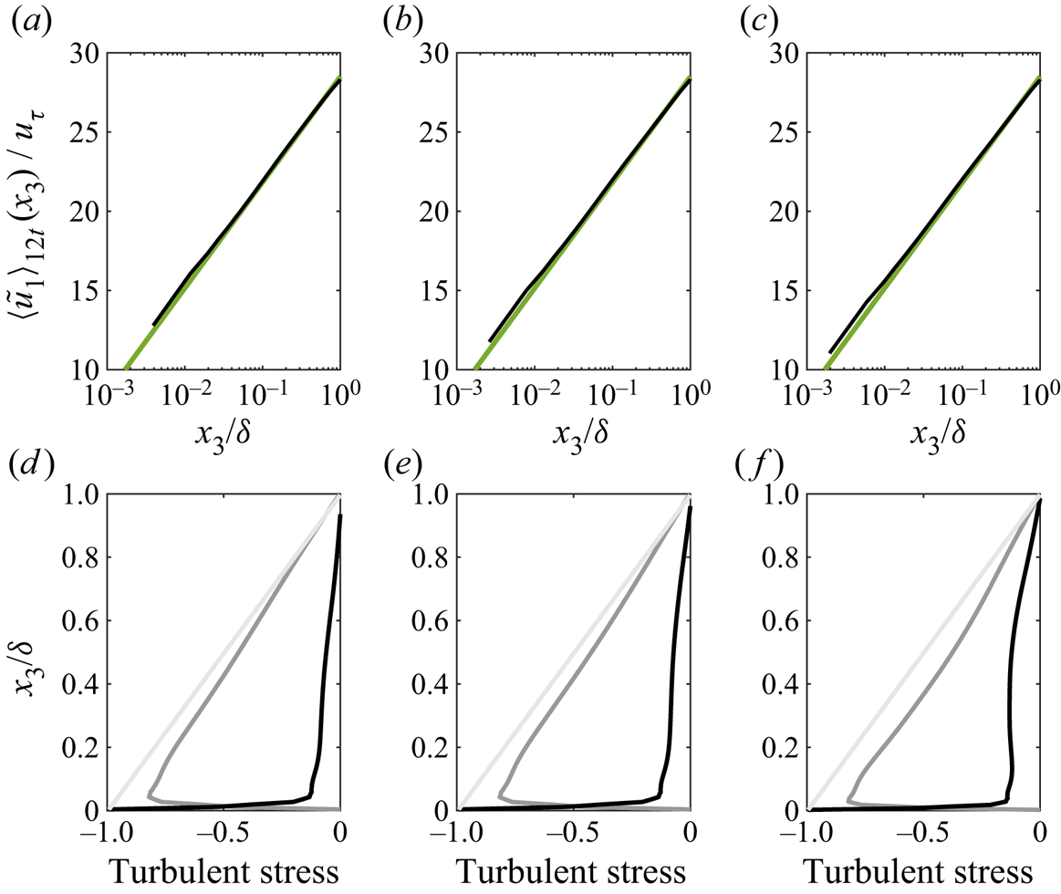
Figures 2(a), 2(b) and 2(c) show vertical profiles of time- and plane-averaged streamwise velocity for cases A, B and C, respectively (case attributes are defined in table 1). For clarity, the wall-normal elevation (abscissa) is shown in logarithmic scale, and in all cases it is clear that the equilibrium (logarithmic) conditions have been attained. Moreover, the profiles agree closely, illustrating resolution insensitivity in first-order flow quantities. Note also that a logarithmic profile can be fitted to the LES profiles a posteriori to recover an effective roughness length,  $U(x_3)/u_\tau = \kappa ^{-1} \log ( x_3 / \ell _{Eff.} )$; results indicate that
 $\ell _{Eff.}/\delta \approx \ell / \delta$, providing further support for the LES results used herein.
First- and second-order turbulence statistics recovered a posteriori from LES of the cases in table 1. Vertical profiles of plane- and time-averaged (a–c) streamwise velocity and (d–e) streamwise–wall-normal stresses, for cases A (a,d), B (b,e) and C (c,f). In (a–c), green profile denotes logarithmic profile for predefined roughness length,  $\ell /\delta = 1 \times 10^{-5}$, which is identical to the prescribed roughness length with each LES (see also § 3). In (d–f) profile colours correspond to: subgrid-scale stress,
 $\langle \tau _{13} \rangle _{12t} / u_\tau ^{2} (x_3)$ (black); resolved stresses,
 $\langle \tilde {u}_1^{\prime } \tilde {u}_3^{\prime } \rangle _{12t} /u_\tau ^{2} (x_3)$ (grey); and total stresses,
 $\langle \mathsf T_{13} \rangle _{12t} / u_\tau ^{2} (x_3) = \langle \tilde {u}_1^{\prime } \tilde {u}_3^{\prime } \rangle _{12t} / u_\tau ^{2} (x_3) + \langle \tau _{13} \rangle _{12t} /u_\tau ^{2} (x_3)$ (light grey). Resolved fluctuations are defined via standard protocols for channel turbulence,
 $\widetilde {\boldsymbol u}^{\prime } = \widetilde {\boldsymbol u} - \langle \widetilde {\boldsymbol u} \rangle _{12t}$.

Figure 2(d–f) shows vertical profiles of time- and plane-averaged streamwise–wall-normal turbulent (Reynolds) stresses, which are recovered a posteriori via addition of the resolved and subgrid-scale stresses,  $\langle \mathsf T_{13} \rangle _{12t}/u_\tau ^{2} = \langle \tilde u_1^{\prime } \tilde u_3^{\prime } \rangle _{12t}/u_\tau ^{2} + \langle \tau _{13} \rangle _{12t}/u_\tau ^{2}$. Figures 2(d), 2(e) and 2(f) show results for cases A, B and C, respectively, where individual case details are summarized in table 1. Inspection of the panels demonstrates, firstly, that all LES cases have been numerically advanced for sufficient time to capture a balance of momentum between the imposed forcing and opposing surface stress, i.e.
 $\langle \mathsf T_{13} \rangle _{12t}/\rho u_\tau ^{2} = - 1$. In addition, we observe correct trends in the relative contributions via the resolved (dark grey) and subgrid-scale stresses (black), where, by definition, the resolved stresses are zero at the wall. These results are consistent with those of prior studies (Bou-Zeid et al. Reference Bou-Zeid, Meneveau and Parlange2005; Anderson & Meneveau Reference Anderson and Meneveau2010).
4.2. Instantaneous streamwise velocity
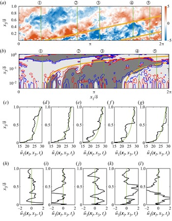
Having established resolution insensitivity and underlying efficacy of the LES code in the preceding section, we transition now to focus on dynamics of UMZs and fidelity of the wake-scaling arguments reviewed in § 2. Figure 3(a,b) shows an arbitrarily selected instantaneous streamwise–wall-normal transect of grid-filtered streamwise velocity fluctuation,  $\tilde {u}_1^{\prime } = \tilde {u}_1 - \langle \tilde {u}_1 \rangle _t$, for case C. Figure 3(a) shows the colourflood contour of
 $\tilde {u}_1^{\prime }$ with both axes shown in linear scaling, while in figure 3(b) the ordinate axis is shown in logarithmic scale. In figure 3(b), regions of
 $\tilde {u}_1^{\prime } < 0$ and
 ${>}0$ are shaded with dark and light grey, respectively, for illustrative purposes; note also that isocontours of positive and negative vertical gradients of
 $\tilde {u}_1^{\prime }$ are also shown, to illustrate interfacial shear between successive UMZs. In both panels, we have superimposed the inclination line associated with a prototypical LSM,
 $\gamma = 16^{\circ }$ (Marusic & Heuer Reference Marusic and Heuer2007). From figure 3(a,b), a clear parcel of inclined, relative momentum excess is anchored to the wall at
 $0 \lesssim x_1 \lesssim 1$ and is elongated above a parcel of relative momentum deficit over region
 $1 \lesssim x_1 \lesssim 3 {\rm \pi}/ 2$. Figure 3(b) illustrates that the observed outer-layer structure continues to the lowest-resolved levels of the computational domain.
Instantaneous velocity data from case C (table 1). Colourflood contours of resolved streamwise velocity fluctuations with (a) linear and (b) logarithmic ordinate scaling. In (a), the complete range of  $\tilde {u}^\prime$ values at the arbitrary time step are shown; isocontours of the limiting 5 % values of vorticity thickness (equation (4.1)) are superimposed, for perspective, where
 $\delta _\omega$ has been signed by the local gradient and where positive and negative values correspond to solid black and solid grey isocontours, respectively. In (b), for perspective, zones of
 $\tilde {u}^\prime < 0$ and
 $\tilde {u}^\prime > 0$ are shown with solid zones of dark and light grey, respectively, with isocontours of
 $\partial _3 \tilde {u}_1^\prime = 1$ (red) and
 $\partial _3 \tilde {u}_1^\prime = -0.2$ (blue) included for perspective. In (a,b), solid yellow lines denote inclination angle,
 $\gamma = 16^{\circ }$ (Marusic & Heuer Reference Marusic and Heuer2007). Instantaneous (c–g) streamwise and (h–l) vertical velocity profiles at locations
 ${\bigcirc{\kern-6pt 1}}$ to
 ${\bigcirc{\kern-6pt 5}}$ (locations denoted by vertical green lines in (a,b)). In (c–g) and (h–l), green profiles correspond to Reynolds-average streamwise velocity profile (logarithmic, based on
 $\ell /\delta = 1 \times 10^{-5}$, see also figure 2(a–c) and accompanying discussion) and vertical velocity profile (
 $\langle \tilde {u}_3 \rangle _{12t}(x_3) = 0$), respectively.

In figure 3(a,b), we have arbitrarily selected a series of streamwise locations ( ${\bigcirc{\kern-6pt 1}}$ to
 ${\bigcirc{\kern-6pt 5}}$) at which profiles of
 $\tilde {u}_1 ({\boldsymbol x}_l, x_3, t)$ and
 $\tilde {u}_3 ({\boldsymbol x}_l, x_3, t)$ are shown (
 ${\boldsymbol x}_l$ denotes an arbitrary location in the
 $x_1$–
 $x_2$ plane; profiles shown in figure 3c–l). This approach has been utilized previously by others, as it provides clear illustration of the ‘staircase’ pattern in
 $\tilde {u}_1 ({\boldsymbol x}_l, x_3, t)$ with increasing
 $x_3$ (de Silva et al. Reference de Silva, Philip, Hutchins and Marusic2017; Bautista et al. Reference Bautista, Ebadi, White, Chini and Klewicki2019; Anderson & Salesky Reference Anderson and Salesky2021). In figure 3(a), we have superimposed the limiting 5 % values of vorticity thickness, signed by the local vertical gradient in streamwise vorticity – thereby revealing retro- and prograde vortices in the interfacial zones (Heisel et al. Reference Heisel, de Silva, Hutchins, Marusic and Guala2021). The signed isocontours of vorticity thickness in figure 3(a) confirm that interfacial shear between successive UMZs represents a distinct signal that coexists within the distribution of length scales associated with ambient shear.
At location  ${\bigcirc{\kern-6pt 1}}$ (figure 3c,h), two notable ‘steps’ are evident at
 $x_3/\delta \approx 0.3$ (excess to deficit) and 0.75 (deficit to excess), where the former and latter correspond to positive and negative gradients, respectively, across the relative momentum deficit. This can be appreciated from figure 3(c), too, with a pronounced region of momentum deficit – relative to the Reynolds average – across the depth of the flow. As might be expected given the overwhelming dominance of anti-correlated motion in the production of turbulence, regions of relative streamwise momentum excess and deficit correspond to regions of relative vertical momentum deficit and excess, respectively (Wallace (Reference Wallace2016) and references therein). These anti-correlated dynamics – termed sweeps and ejections for motions with aggregate
 $\{\tilde {u}_1 ({\boldsymbol x} , t), \tilde {u}_3 ({\boldsymbol x} , t)\} \equiv \{ >0,<0 \}$ and
 $\equiv \{<0,>0\}$, respectively – have been thoroughly addressed in prior studies and are not further reviewed here.
The lowest step observed at location  ${\bigcirc{\kern-6pt 1}}$ is the lower bound of a UMZ interface observed at
 $x_3/\delta \approx 0.2$ (location
 ${\bigcirc{\kern-6pt 2}}$),
 $\approx 0.4$ (location
 ${\bigcirc{\kern-6pt 3}}$) and
 $\approx 0.5$ (location
 ${\bigcirc{\kern-6pt 4}}$); a large-scale undulation at location
 ${\bigcirc{\kern-6pt 5}}$ precludes continuation of the inclined interface, although abrupt gradients are nevertheless evident. The aforementioned UMZ interface – and associated band of elevated shear – is above and below a region of relative momentum deficit and excess, respectively. As noted, the accompanying vertical velocity attributes are consistent with preceding insights on relative dominance of sweeps and ejections in the production of turbulence.
Note, finally, that the instantaneous results presented in figure 3(c–l) provide rudimentary support for the wake-scaling arguments outlined in § 1. That is, we observe a general attenuation in the amplitude of streamwise velocity increases with increasing wall-normal location – as per (2.20). In contrast, the relative incremental variation in vertical velocity does not exhibit such monotonic attenuation with  $x_3$ – at least based on the instantaneous results shown – and this result is consistent with (2.23) (exhaustive results are shown in subsequent sections).
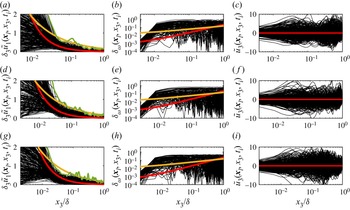
To further the analysis, in figure 4 we show a random sampling of vertical profiles of  $\partial _3 \tilde {u}_1 ({\boldsymbol x}_l,x_3,t)$ (figure 4a,d,g), vorticity thickness
 \begin{equation} {\delta_\omega ({\boldsymbol x}_l,x_3,t)} = \frac{| \delta {\tilde{u}_1 ({\boldsymbol x}_l,x_3,t)}|}{\underbrace{\textrm{max}}_{12} (|\partial_3 \tilde{u}_1 ({\boldsymbol x}_l,x_3,t)|)} \end{equation}
(figure 4b,e,h) and vertical velocity (figure 4c,f,i). Note that the numerator in (4.1),  $\delta \tilde {u}_1 ({\boldsymbol x}_l,x_3,t)$, is based on the absolute value of the spatial difference in the vertical direction (the absolute value is required given the resultant quantity is a length). The profiles are based on an arbitrary sampling in time and in the
 ${\boldsymbol x}_l = \{x_{1,l},x_{2,l} \}$ plane. Superimposed on figure 4(a,d,g) and figure 4(c,f,i) are the Reynolds-averaged profiles,
 $\mathrm {d}_3 \langle \tilde {u}_1 \rangle _{12t} (x_3) = u_\tau / (\kappa x_3)$ and
 $\langle \tilde {u}_3 \rangle _{12t} (x_3) = 0$, respectively (red lines). For perspective, a notional Reynolds-averaged vorticity thickness is superimposed,
 $\langle \delta _\omega \rangle _{12t} (x_3)/\delta \approx (x_3/\delta ) \log (1 + \delta _3 x / x_3) \approx C_1 x_3/\delta$ for small
 $\delta _3 x$, where
 $C_1$ is a dimensionless constant. With the obvious exception of vertical velocity, it is clear that these shear-based quantities instantaneously depart from Reynolds-averaged predictions.
Vertical profiles of instantaneous velocity statistics from an arbitrary survey of streamwise–spanwise locations for cases A (a–c), B (d–f) and C (g–i), for (a,d,g)  $\partial _3 \tilde {u}_1 ({\boldsymbol x}_l,x_3,t_i)$, (b,e,h) vorticity thickness (4.1) and (c,f,i) vertical velocity,
 $\tilde {u}_3 ({\boldsymbol x}_l,x_3,t_i)$. In all panels, red lines denote Reynolds-averaged profiles, i.e.
 $\mathrm {d}_3 \langle \tilde {u}_1 \rangle _{12t} (x_3) = u_\tau /(\kappa x_3) \sim x_3^{-1}$ (a,d,g),
 $\langle \delta _\omega \rangle _{12t} (x_3) = C x_3 \sim x_3$ (b,e,h), where
 $C$ is a proportionality constant used only for the purpose of illustration, and
 $\langle \tilde {u}_3 \rangle _{12t} (x_3) = 0$ (c,f,i). In (a,d,g), green profile represents the maximum value of
 $\partial _3 \tilde {u}_1 ({\boldsymbol x}_l,x_3,t_i)$ at each elevation. In addition, yellow profiles in (a,d,g) and (b,e,h) correspond to
 $\partial _3 \tilde {u}_1 ({\boldsymbol x}_l,x_3,t_i) \sim x_3^{-1/2}$ and
 $\delta _\omega \sim x_3^{1/2}$, respectively. The results in (a,d,g) and (c,f,i) are consistent with (2.20) and (2.15a,b), respectively.

In figure 4(a,d,g), the green profile denotes the silhouette of maximum values – which departs sharply from logarithmic (equilibrium) scale arguments – but does so in a repeatable manner: in fact, the accompanying yellow profile denotes  $C_2 x_3^{-1/2}$, where
 $C_2$ is an amplitude. Recall that the wake-scaling arguments yield the result
 $\partial _3 \tilde {u}_1 \sim x_3^{-1/2}$, which thus agrees with the fitted profile,
 $C_2 x_3^{-1/2}$ (Anderson & Salesky Reference Anderson and Salesky2021). This result lends further support to the underlying argument that UMZs are the consequence of structure collisions in the sublayer, which yield the plumes of quasi-uniform momentum observed as UMZs. This structure necessitates the narrow bands of interfacial shear, with shear intensity declining monotonically with
 $x_3$ as the structural coherence homogenizes due to ambient shear.
In figure 4(b,e,h), we leverage the figure 4(a,d,g) result that  $\partial _3 \tilde {u}_1 \sim x_3^{-1/2}$ by providing the line
 $\delta _\omega \sim x_3^{1/2}$ (yellow), which agrees closely against the reported vorticity thickness profiles. Note, also, that
 $\delta _\omega \sim x_3^{1/2}$ is a necessary consequence of the wake-scaling arguments (equation (2.15a,b) and accompanying text) outlined in Tennekes & Lumley (Reference Tennekes and Lumley1972). Finally, to further integrate the LES results against the wake-scaling arguments, figure 4(c,f,i) shows a sampling of
 $\tilde {u}_3 ({\boldsymbol x}_l,x_3,t)$. Note that the amplitude of
 $\tilde {u}_3 ({\boldsymbol x}_l,x_3,t)$ variability does not exhibit significant
 $x_3$ dependence for
 $x_3/\delta \gtrsim 10^{-1}$. This result is also consistent with deductions from the wake-scaling framework (equation (2.23) and accompanying text). Note that vertical profiles of resolved vertical velocity variance,
 $\langle (\tilde {u}_3^{\prime })^{2} \rangle _{12t}(x_3)$, do exhibit the expected wall-normal decay (Anderson & Meneveau Reference Anderson and Meneveau2010).
Figure 4 provides further evidence of monotonic trends of turbulence statistics, since figures 4(a–c), 4(d–f) and 4(g–i) correspond to results from LES of cases A, B and C (table 1).
4.3. Conditionally averaged results
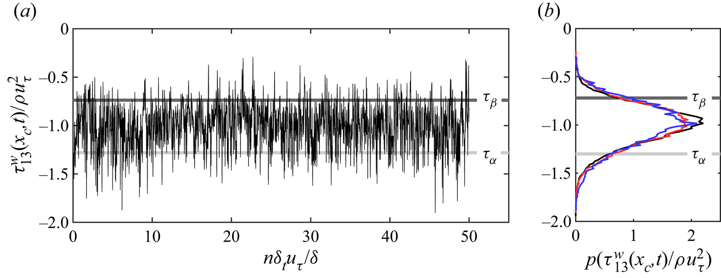
In order to isolate structural attributes of UMZs with greater clarity, we have used conditional-sampling protocols outlined below. Conditional sampling has been used frequently in such studies (Antonia Reference Antonia1981; Sheng, Malkiel & Katz Reference Sheng, Malkiel and Katz2009; Hutchins et al. Reference Hutchins, Monty, Ganapathisubramani, Ng and Marusic2011); in fact, Jacob & Anderson (Reference Jacob and Anderson2017) used conditional sampling to highlight the correlation between large-scale outer-layer motions and surface stress. Given the focus of this article – sublayer and outer-layer structure – we have used an approach similar to that of Jacob & Anderson (Reference Jacob and Anderson2017) here. Figure 5(a) shows time-series evolution of local surface stress for case B (comparable time-series visualization for cases A and C is omitted for brevity), where the relatively less and more negative values are known to correlate with low- and high-momentum regions aloft (Jacob & Anderson Reference Jacob and Anderson2017). To provide more detail of the time-series attributes, figure 5(b) shows probability density functions for cases A, B and C (line colour coding defined in the caption).
Statistics of space-local surface stress,  $\tau _{13}^{w} ({\boldsymbol x}_c,t)/\rho u_\tau ^{2}$, at central location,
 ${\boldsymbol x}_c = \{L_1/2, L_2/2 \}$. (a) Results for case B over an arbitrary sampling period during LES. (b) Resultant probability density function for all cases, where black, red and blue lines correspond to cases A, B and C. In both panels, light and dark grey lines illustrate sampling thresholds,
 $\tau _\alpha$ and
 $\tau _\beta$, respectively, used in subsequent conditional sampling (equation (4.2a,b); discussed in the text).

As has been widely reported, local stress exhibits large variability and is skewed towards low-probability, high-impact events (Jacob & Anderson Reference Jacob and Anderson2017). Indeed, Jacob & Anderson (Reference Jacob and Anderson2017) demonstrated that large-scale deviation in surface stress from its Reynolds-average value correlates precisely with the presence of LSMs aloft (this group quantified a wide range of conditionally sampled flow attributes, all of which supported the premise that LSMs correlated with the presence of stress excursions). Note that this result is supported by literature on amplitude modulation/correlation, wherein LSMs aloft correlate strongly with inner-layer processes (amplitude and frequency of quantities relevant to surface stress; Mathis et al. Reference Mathis, Hutchins and Marusic2009; Marusic et al. Reference Marusic, Mathis and Hutchins2010; Mathis et al. Reference Mathis, Marusic, Chernyshenko and Hutchins2013; Anderson Reference Anderson2016). It is for this reason that we also use surface stress as a ‘triggering’ event for the recovery of LSMs. In order to isolate attributes of large-scale momentum excesses and deficits, we nominate thresholds  $\tau _\alpha$ and
 $\tau _\beta$, respectively; both thresholds are graphically indicated in figure 5, where the thresholds correspond to relatively low-probability, high-impact activity. The conditional-sampling protocols are imposed via the following:
 \begin{align} \langle \widetilde{\boldsymbol u} \rangle_\alpha ({\boldsymbol x}) = \langle \widetilde{\boldsymbol u}(\boldsymbol x,t)| \tau_{13}^{w} (\boldsymbol x_c,t) \le \tau_\alpha \rangle_{N_\alpha}\quad\textrm{and}\quad \langle \widetilde{\boldsymbol u}\rangle_\beta ({\boldsymbol x}) = \langle \widetilde{\boldsymbol u}(\boldsymbol x,t)| \tau_{13}^{w} (\boldsymbol x_c,t) \ge \tau_\beta \rangle_{N_\beta}, \end{align}
where  $N_\alpha$ and
 $N_\beta$ are the number of ensembles associated with exceedance of the predefined surface stress triggers.
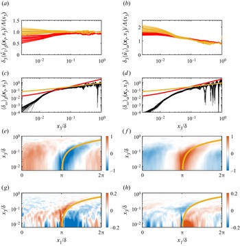
Results from application of (4.2a,b) sampling protocols are presented in figure 6. Results are shown only for case B (table 1). Results of comparison against conditionally sampled results for cases A and C show no discernible variability, and as such these results were omitted for brevity; likewise, it is noted that selection of differing thresholds does not materially affect structural attributes and associated scientific conclusions. Figures 6(a) and 6(b) show vertical profiles of the vertical gradient of  $\langle \tilde {u}_1 \rangle _\beta$ and
 $\langle \tilde {u}_1 \rangle _\alpha$, respectively; the yellow and red profiles are based upon normalization by
 $\varLambda (x_3) = A x_3^{-1/2}$ and
 $\varLambda (x_3) = A x_3^{-1}$, respectively. Readers are reminded that
 $\varLambda (x_3) = A x_3^{-1/2}$ captures the wall-normal scaling dependence of interfacial shear under the wake-scaling arguments (equation (2.20), figure 4a,d,g);
 $\varLambda (x_3) = A x_3^{-1}$ is the wall-normal scaling argument under equilibrium (logarithmic) conditions (equation (1.1a,b)). It is immediately clear that shear embodied within the conditionally sampled structures is poorly captured by the logarithmic law, but does agree closely with predictions based on wake-scaling arguments. This lends further support to the conceptual depiction outlined in figure 1 and accompanying text. It is notable that the conditionally sampled flow departs from logarithmic conditions for
 $\tau _\alpha$ and
 $\tau _\beta$; for
 $\tau _\alpha$, wake-scaling arguments are also weak for
 $x_3/\delta \lesssim 10^{-1}$. Note, however, that
 $\tau _\alpha$ corresponds to the presence of a relative momentum excess aloft the sampling point. As per figure 1 and accompanying discussion, the entire development is predicated upon bluff-body-like interactions between relative momentum excesses and deficits, so wake-scaling arguments are not expected to be realized for sampling based on
 $\tau _\alpha$.
Conditionally averaged results for case B based on application of the conditional-sampling protocols outlined with (4.2a,b) for  $\tau _\beta$ (a,c,e,g) and
 $\tau _\alpha$ (b,d,f,h). (a,b) Vertical gradient of conditionally sampled streamwise velocity normalized by
 $\varLambda = A x_3^{-1/2}$ (yellow lines) and
 $\varLambda = B x_3^{-1}$ (red lines), where
 $A$ and
 $B$ are proportionality constants used only to illustrate dependence upon
 $x_3$. (c,d) Conditionally sampled vorticity thickness alongside profiles
 $A x_3^{1/2}$ (yellow lines) and
 $B x_3^{1}$, where
 $A$ and
 $B$ are proportionality constants used only to illustrate dependence upon
 $x_3$. Colourflood contours of (e,f) conditionally sampled streamwise velocity and (g,h) vertical gradient of conditionally sampled streamwise velocity; yellow profile in both denotes structural inclination angle,
 $\gamma = 16^{\circ }$.

Vorticity thickness developed within the conditionally sampled flow departs markedly from equilibrium conditions,  $\sim x_3^{1}$ (red lines in figure 6c,d), but agrees closely with wake-scaling arguments,
 $\sim x_3^{1/2}$. For further clarity, figures 6(e,f) and 6(g,h) show conditionally sampled velocity and vertical gradient of conditionally sampled velocity, respectively. As might be expected, a relative deficit and excess in streamwise velocity resides above the sampling point for
 $\tau _\beta$ and
 $\tau _\alpha$. Note, too, that the topology of the sampled structures conforms closely with inclination of LSMs, further supporting results and deductions made herein. Likewise, colourflood contours of the vertical gradient of
 $\langle \tilde {u}_1 \rangle _\beta$ and
 $\langle \tilde {u}_1 \rangle _\alpha$ are shown in figures 6(g) and 6(h), respectively. For
 $\partial _3 \langle \tilde {u}_1 \rangle _\beta$, the narrow band of elevated shear encompasses the momentum deficit, which is the interfacial shear between successive UMZs. The results for
 $\partial _3 \langle \tilde {u}_1 \rangle _\alpha$ (figure 6h) are consistent with figure 6(f), but again it is noted that this conditional sampling does not capture the conditions thought to initiate UMZs under the wake-scaling arguments.
5. Concluding remarks
The flow physics associated with UMZs has received significant attention from the community (Meinhart & Adrian Reference Meinhart and Adrian1995), particularly in recent years (de Silva et al. Reference de Silva, Philip, Hutchins and Marusic2017; Laskari et al. Reference Laskari, de Kat, Hearst and Ganapathisubramani2018; Bautista et al. Reference Bautista, Ebadi, White, Chini and Klewicki2019; Heisel et al. Reference Heisel, de Silva, Hutchins, Marusic and Guala2020; Montemuro et al. Reference Montemuro, White, Klewicki and Chini2020; Heisel et al. Reference Heisel, de Silva, Hutchins, Marusic and Guala2021). Such UMZs,  $\delta$-scale regions of quasi-uniform momentum, are inclined in the streamwise direction and encompassed by bands of elevated shear in the interfacial regions separating adjacent structures. Recently, Anderson & Salesky (Reference Anderson and Salesky2021) leveraged access to a transformative DNS dataset to study instantaneous three-dimensional attributes of UMZs for inertia-dominated channel turbulence (Lee & Moser Reference Lee and Moser2015). The results and insights were framed in the context of pre-existing arguments on the structure of inertia-dominated turbulent wakes (Tennekes & Lumley Reference Tennekes and Lumley1972). In this sense, Anderson & Salesky (Reference Anderson and Salesky2021) argue that bluff-body-like collisions within the autonomous cycle yield regions of quasi-uniform momentum, which manifest as UMZs as time advances. These results were all based on insights from DNS, but a great many flows of practical importance exhibit inertial conditions requiring LES.
For this article, details of the wake-scaling arguments were reviewed for asymptotic  $Re_\tau$ channel turbulence conditions. In addition, attributes of the development were further advanced for new predicted scaling arguments. Also, LES was used to model asymptotic
 $Re_\tau$ channel turbulence, which thus precludes resolution of the inner cycle (instead, the lowest
 $\approx$10 % of the domain is occupied by a roughness/inner layer). Nevertheless, we find that the underlying wake-scaling arguments agree closely against predictions from LES. The perception of a harmonious transition from deductions realized via DNS and LES is, of course, regulated by LES resolution. Herein, we have used carefully designed LES cases that are able to capture UMZ interfaces within the computational mesh, thus resolving inertial-range processes and ensuring modelled subgrid-scale effects associated with descendent processes. And results presented herein illustrate insensitivity of the results to three computational mesh resolutions considered. In the transition to an unsteady-Reynolds-averaged treatment, such flow structures – and deductions presented here – would not be realized.
It is stressed once more that the arguments underpinning this work – bluff-body-like interactions generate inertial-layer wakes that manifest as UMZs – are presented as a candidate explanation for observed dynamics in wall-sheared turbulence. This presupposed existence of a ‘bottom up’ hierarchy is itself the topic of ongoing work, and there are formidable counter arguments to these suppositions (e.g. Hwang & Cossu Reference Hwang and Cossu2010; Dong et al. Reference Dong, Lozano-Duran, Sekimoto and Jimenez2017).
Funding
This work was supported by AFOSR grant no. FA9550-19-1-0134 (W.A.). High-performance computing resources were provided by the Texas Advanced Computing Center at the University of Texas.
Declaration of interests
The authors report no conflict of interest.