1 Introduction
In microfluidic devices, manipulation of the flow and the suspended phases such as cells, droplets/bubbles, macromolecules (for example, DNAs), etc. is commonly needed. The flow manipulation includes mixing, pumping, valving, sensing and related operations. In order to achieve these functions, different strategies have been developed. One of the most intuitive approaches is to introduce into the microfluidic device a rotary element, whose rotation is achieved by applying an external electric (Bart et al. Reference Bart, Mehregany, Tavrow, Lang and Senturia1992) or magnetic field (Ahn & Allen Reference Ahn and Allen1995; Döpper et al. Reference Döpper, Clemens, Ehrfeld, Jung, Kaemper and Lehr1997; Ryu et al. Reference Ryu, Shaikh, Goluch, Fan and Liu2004; Agarwal et al. Reference Agarwal, Sridharamurthy, Beebe and Jiang2005; van den Beld et al. Reference van den Beld, Cadena, Bomer, de Weerd, Abelmann, van den Berg and Eijkel2015). On the other hand, such elements are also able to rotate passively without resorting to any external fields, but propelled by the underlying flow alone if they are placed asymmetrically with respect to the flow. This approach has been demonstrated by Zaki, Sen & Gad-el-Hak (Reference Zaki, Sen and Gad-el-Hak1994) and Day & Stone (Reference Day and Stone2000), where the latter was inspired by the experimental work of rotating an asymmetrically placed cylinder to pump fluid in a duct (Sen, Wajerski & Gad-el-Hak Reference Sen, Wajerski and Gad-el-Hak1996). More recently, Moon, Tsai & Hwang (Reference Moon, Tsai and Hwang2015) have succeeded in driving rotary microgears by the underlying flow in a microfluidic channel. Each of their microgears consisted of eight paddles equally spaced in angle, and was fabricated and installed via in situ polymerisation based on flow lithography. The authors also showed that a pair of microgears was able to transmit the hydrodynamic torque from one gear to the other. Likewise, a similar flow-driven wheel was implemented by Attia (Reference Attia2008) (PhD thesis in French) as a flow sensor to measure the flow speed in a microfluidic channel.
Motivated by such microfluidic experiments, we hereby carry out a theoretical and numerical study on the low-Reynolds-number hydrodynamics of such flow-driven rotary devices resembling micro-scale ‘watermills’. We aim to provide design principles for their applications in microsystems. After presenting the problem set-up in § 2, we describe in § 3 the methodologies including the classical resistive force (RF) theory and numerical methods. The results obtained are compared in § 4, which identifies the role of hydrodynamic interactions absent from the classical RF theory. Therefore, an improved RF theory taking hydrodynamic interactions into account is developed in § 5.1 based on the recent theoretical work of Man, Koens & Lauga (Reference Man, Koens and Lauga2016). We use the improved theory to solve the resistance and mobility problems of a simplified version of the watermill, and compare the theoretical predictions with the numerical results. Finally, we conclude and discuss our results in § 6.
2 Problem set-up
We consider a watermill-like rotary device consisting of
 $N\geqslant 1$
cylindrical rods equally distributed in a plane in the azimuthal direction (see figure 1). The angle between two successive rods is
 $\unicode[STIX]{x1D719}=2\unicode[STIX]{x03C0}/N$
. All of the rods are jointed on a common end on the rotation axis of the device that is along the
 $z$
direction. Hence the device rotates in the horizontal
 $xy$
plane. The length of a rod is
 $L$
, with its circular cross-section of radius
 $a$
, and the slenderness of the rod is defined as
 $\unicode[STIX]{x1D716}=a/L\ll 1$
. We place the watermill in an unbounded Poiseuille flow
 $\boldsymbol{U}^{\infty }=U_{0}(1-x^{2}/R^{2})\boldsymbol{e}_{y}$
, with the position
 $\boldsymbol{x}_{joint}$
of the watermill’s joint (rotation axis) away from the centre (
 $x=0$
) of the flow domain by distance
 $b\geqslant 0$
, i.e.
 $\boldsymbol{x}_{joint}=b\boldsymbol{e}_{x}$
. Two non-dimensional parameters
 $$\begin{eqnarray}\displaystyle & \unicode[STIX]{x1D6FD}=b/L, & \displaystyle\end{eqnarray}$$
 $$\begin{eqnarray}\displaystyle & \unicode[STIX]{x1D70C}=R/L, & \displaystyle\end{eqnarray}$$
 $\unicode[STIX]{x1D703}$
between the first rod (arbitrarily labelled without losing generality) and the
 $x$
-axis. The rotational velocity
 $\unicode[STIX]{x1D714}_{z}=\,\text{d}\unicode[STIX]{x1D703}/\text{d}t$
of the watermill depends on its orientation
 $\unicode[STIX]{x1D703}\in [0,\unicode[STIX]{x1D719}]$
.
The dynamic viscosity of the fluid is
 $\unicode[STIX]{x1D707}$
. We choose
 $U_{0}$
,
 $L$
,
 $L/U_{0}$
,
 $\unicode[STIX]{x1D707}U_{0}/L$
,
 $\unicode[STIX]{x1D707}U_{0}L$
and
 $\unicode[STIX]{x1D707}U_{0}L^{2}$
as, respectively the characteristic velocity, length, time, stress, force and torque. Non-dimensional quantities are denoted by ¯ from hereafter. We fix
 $\unicode[STIX]{x1D716}=0.02$
in this study.
A watermill free to rotate in an underlying Poiseuille flow. (a) Sketch of an anchored, freely rotating watermill comprised of
 $N$
rigid cylindrical rods equally spaced in angle. The motion is driven by an unbounded Poiseuille flow
 $\boldsymbol{U}^{\infty }$
. (b) The rotation axis of the watermill is aligned in the
 $z$
direction and is away from the centre of the flow by a distance
 $b$
in the
 $x$
direction.

3 Methodologies
We carry out our study in the low-Reynolds-number flow regime and thus solve the Stokes equations. By employing the classical resistive force (RF) theory, we calculate the rotational velocities of a freely rotating watermill consisting of equally spaced rods. In § 4, the results are compared with those computed by direct numerical simulations of the Stokes equations. The comparisons indicate that inter-rod hydrodynamic interactions neglected by the RF theory play an important role in certain configurations. This feature thus motivates us to conduct a theoretical study adopting the recently developed RF-based mathematical framework of Man et al. (Reference Man, Koens and Lauga2016) that accounts for hydrodynamic interactions; this ‘RF-HI’ theory will be described in § 5. The classical RF theory and numerical methods are documented in §§ 3.1 and 3.2, respectively.
3.1 Classical resistive force theory
We define an arclength
 $s\in [0,L]$
on each rod, with
 $s=0$
and
 $s=L$
corresponding to the joint and free end, respectively. The RF theory dictates that the hydrodynamic force per unit length
 $\boldsymbol{f}^{(k)}$
exerted by the fluid on the
 $k$
th rod is a function of the arclength
 $s$
according to
 $$\begin{eqnarray}\displaystyle \boldsymbol{f}^{(k)}(s)=-\unicode[STIX]{x1D645}^{(k)}\boldsymbol{\cdot }\left[\frac{\unicode[STIX]{x2202}\boldsymbol{r}^{(k)}}{\unicode[STIX]{x2202}t}-\boldsymbol{U}^{\infty }(\boldsymbol{r}^{(k)})\right], & & \displaystyle\end{eqnarray}$$
where
 $\boldsymbol{r}(s)$
and
 $\boldsymbol{t}(s)=\unicode[STIX]{x2202}\boldsymbol{r}/\unicode[STIX]{x2202}s$
denote, respectively, the local coordinates and tangent of the rod’s centreline;
 $\unicode[STIX]{x1D645}(\boldsymbol{t})=\unicode[STIX]{x1D709}_{\bot }\unicode[STIX]{x1D644}+(\unicode[STIX]{x1D709}_{\Vert }-\unicode[STIX]{x1D709}_{\bot })\boldsymbol{t}\boldsymbol{t}$
, where
 $\unicode[STIX]{x1D709}_{\bot }$
and
 $\unicode[STIX]{x1D709}_{\Vert }$
are the drag coefficients for the motion of rod in the directions perpendicular and parallel to
 $\boldsymbol{t}$
. Note that
 $\unicode[STIX]{x1D709}_{\bot }=2\unicode[STIX]{x1D709}_{\Vert }\approx 4\unicode[STIX]{x03C0}\unicode[STIX]{x1D707}/\ln \unicode[STIX]{x1D716}^{-1}$
(Lighthill Reference Lighthill1975).
The hydrodynamic torque exerted on the
 $k$
th rod about the joint is
 $\boldsymbol{T}^{(k)}=\int _{0}^{L}(\boldsymbol{r}^{(k)}-\boldsymbol{x}_{joint})\times \boldsymbol{f}^{(k)}\,\text{d}s$
. Since the watermill only rotates in the
 $xy$
plane, we only consider the
 $z$
-component of the torque on the
 $k$
th rod, whose non-dimensional value is
 $$\begin{eqnarray}\bar{T}_{z}^{(k)}=\frac{1}{3\unicode[STIX]{x1D70C}^{2}\ln \unicode[STIX]{x1D716}^{-1}}[6(\unicode[STIX]{x1D6FD}^{2}-\unicode[STIX]{x1D70C}^{2})\cos \unicode[STIX]{x1D703}^{(k)}+8\unicode[STIX]{x1D6FD}\cos ^{2}\unicode[STIX]{x1D703}^{(k)}+3\cos ^{3}\unicode[STIX]{x1D703}^{(k)}+4\unicode[STIX]{x1D70C}^{2}\bar{\unicode[STIX]{x1D714}}_{z}],\end{eqnarray}$$
where
 $\bar{\unicode[STIX]{x1D714}}_{z}$
is the non-dimensional rotational velocity of the watermill;
 $\unicode[STIX]{x1D703}^{(k)}$
denotes the angle between the
 $k$
th rod and the
 $x$
-axis and
 $\unicode[STIX]{x1D703}^{(1)}=\unicode[STIX]{x1D703}$
. The total torque on the rotary device,
 $\bar{T}_{z}=\sum _{k=1}^{N}\bar{T}_{z}^{(k)}$
, from which we find
 $$\begin{eqnarray}\displaystyle 3\unicode[STIX]{x1D70C}^{2}(\ln \unicode[STIX]{x1D716}^{-1})\bar{T}_{z} & = & \displaystyle \mathop{\sum }_{k=1}^{N}\left\{\left[6(\unicode[STIX]{x1D6FD}^{2}-\unicode[STIX]{x1D70C}^{2})+\frac{9}{4}\right]\cos \unicode[STIX]{x1D703}^{(k)}+4\unicode[STIX]{x1D6FD}\cos 2\unicode[STIX]{x1D703}^{(k)}+\frac{3}{4}\cos 3\unicode[STIX]{x1D703}^{(k)}\right\}\nonumber\\ \displaystyle & & \displaystyle +\,4N(\unicode[STIX]{x1D6FD}+\unicode[STIX]{x1D70C}^{2}\bar{\unicode[STIX]{x1D714}}_{z}).\end{eqnarray}$$
Since the rods are equally spaced on a circle, we use the properties of the roots of unity (detailed in appendix A) to obtain
 $$\begin{eqnarray}\displaystyle \mathop{\sum }_{k=1}^{N}\cos \unicode[STIX]{x1D703}^{(k)}=\left\{\begin{array}{@{}ll@{}}\cos \unicode[STIX]{x1D703},\quad & N=1\\ 0,\quad & N\geqslant 2,\end{array}\right. & & \displaystyle\end{eqnarray}$$
 $$\begin{eqnarray}\displaystyle \mathop{\sum }_{k=1}^{N}\cos 2\unicode[STIX]{x1D703}^{(k)}=\left\{\begin{array}{@{}ll@{}}\cos 2\unicode[STIX]{x1D703},\quad & N=1\\ 2\cos 2\unicode[STIX]{x1D703},\quad & N=2\\ 0,\quad & N\geqslant 3,\end{array}\right. & & \displaystyle\end{eqnarray}$$
and
 $$\begin{eqnarray}\displaystyle \mathop{\sum }_{k=1}^{N}\cos 3\unicode[STIX]{x1D703}^{(k)}=\left\{\begin{array}{@{}ll@{}}\cos 3\unicode[STIX]{x1D703},\quad & N=1\\ 0,\quad & N=2\\ 3\cos 3\unicode[STIX]{x1D703},\quad & N=3\\ 0,\quad & N\geqslant 4,\end{array}\right. & & \displaystyle\end{eqnarray}$$
so that the total torque
 $\bar{T}_{z}$
can be written as
 $$\begin{eqnarray}\displaystyle & & \displaystyle 3\unicode[STIX]{x1D70C}^{2}(\ln \unicode[STIX]{x1D716}^{-1})\bar{T}_{z}\nonumber\\ \displaystyle & & \displaystyle \quad =\left\{\begin{array}{@{}ll@{}}[6(\unicode[STIX]{x1D6FD}^{2}-\unicode[STIX]{x1D70C}^{2})+\frac{9}{4}]\cos \unicode[STIX]{x1D703}+4\unicode[STIX]{x1D6FD}\cos 2\unicode[STIX]{x1D703}+\frac{3}{4}\cos 3\unicode[STIX]{x1D703}+4(\unicode[STIX]{x1D6FD}+\unicode[STIX]{x1D70C}^{2}\bar{\unicode[STIX]{x1D714}}_{z}),\quad & N=1\\ 8\unicode[STIX]{x1D6FD}\cos 2\unicode[STIX]{x1D703}+8(\unicode[STIX]{x1D6FD}+\unicode[STIX]{x1D70C}^{2}\bar{\unicode[STIX]{x1D714}}_{z}),\quad & N=2\\ \frac{9}{4}\cos 3\unicode[STIX]{x1D703}+12(\unicode[STIX]{x1D6FD}+\unicode[STIX]{x1D70C}^{2}\bar{\unicode[STIX]{x1D714}}_{z}),\quad & N=3\\ 4N(\unicode[STIX]{x1D6FD}+\unicode[STIX]{x1D70C}^{2}\bar{\unicode[STIX]{x1D714}}_{z}),\quad & N\geqslant 4.\end{array}\right.\nonumber\\ \displaystyle & & \displaystyle\end{eqnarray}$$
The rotational velocity of a freely rotating watermill can be obtained by applying the torque-free condition
 $\bar{T}_{z}=0$
and we find
 $$\begin{eqnarray}\displaystyle \bar{\unicode[STIX]{x1D714}}_{z}=\left\{\begin{array}{@{}ll@{}}-\text{cos}\,\unicode[STIX]{x1D703}[6(\unicode[STIX]{x1D6FD}^{2}-\unicode[STIX]{x1D70C}^{2})+8\unicode[STIX]{x1D6FD}\cos \unicode[STIX]{x1D703}+3\cos ^{2}\unicode[STIX]{x1D703}]/(4\unicode[STIX]{x1D70C}^{2}),\quad & N=1\\ -2\unicode[STIX]{x1D6FD}\cos ^{2}\unicode[STIX]{x1D703}/\unicode[STIX]{x1D70C}^{2},\quad & N=2\\ -[16\unicode[STIX]{x1D6FD}+3\cos 3\unicode[STIX]{x1D703}]/(16\unicode[STIX]{x1D70C}^{2}),\quad & N=3\\ -\unicode[STIX]{x1D6FD}/\unicode[STIX]{x1D70C}^{2},\quad & N\geqslant 4.\end{array}\right. & & \displaystyle\end{eqnarray}$$
3.2 Numerical methods
To determine the rotational velocity of the watermill numerically, we carry out three-dimensional direct numerical simulations (DNS) based on a commercial finite-element method (FEM) solver COMSOL. We have experience in performing COMSOL simulations for viscoelastic flows, for example, Pak et al. (Reference Pak, Zhu, Brandt and Lauga2012), where the propulsion of two touching rotating spheres in viscoelastic fluids was investigated and the numerical results were in excellent agreement with the asymptotic analysis in the small-Deborah-number regime. It is worth noting that prior studies of interacting slender bodies in viscous flows have adopted other numerical implementations (Yamamoto & Matsuoka Reference Yamamoto and Matsuoka1995; Ross & Klingenberg Reference Ross and Klingenberg1997; Saintillan & Shelley Reference Saintillan and Shelley2007; Nazockdast et al. Reference Nazockdast, Rahimian, Zorin and Shelley2017).
Since we assume that the Reynolds number
 $Re=\unicode[STIX]{x1D70C}_{f}U^{\infty }L/\unicode[STIX]{x1D707}$
is small (
 $\unicode[STIX]{x1D70C}_{f}$
denotes the fluid density), inertial effects are negligible, and we solve the non-dimensional steady Stokes equations
 $$\begin{eqnarray}\displaystyle & -\unicode[STIX]{x1D735}\bar{p}+\unicode[STIX]{x1D6FB}^{2}\bar{\boldsymbol{u}}=\mathbf{0}, & \displaystyle\end{eqnarray}$$
 $$\begin{eqnarray}\displaystyle & \unicode[STIX]{x1D735}\boldsymbol{\cdot }\bar{\boldsymbol{u}}=0. & \displaystyle\end{eqnarray}$$
For a channel flow, we impose a Dirichlet boundary condition (BC) with the Poiseuille flow profile in the inlet of the domain and a constant pressure BC at the outlet. Utilising the mirror symmetry of the set-up, we only need to consider the upper half (
 $z\geqslant 0$
) of the domain by applying a symmetry BC at the
 $z=0$
plane. We adopt the same symmetry BC at the
 $z=H_{z}/2$
plane, which effectively corresponds to an array of watermills equally spaced along the
 $z$
direction by distance
 $H_{z}$
. No-slip BCs are specified on the two lateral walls at
 $x=\pm R$
. Since both the RF and RF-HI theories are derived for unbounded flows, i.e. without accounting for wall effects, the boundedness of the computational domain needs to be considered carefully for a reasonable comparison of the theoretical and numerical results. We choose the length
 $H_{y}$
of the domain equal to
 $100L$
. To mitigate the confinement effects of the lateral walls, the characteristic width of the channel flow
 $\unicode[STIX]{x1D70C}=5$
is used in most of our cases. We have varied the distance
 $H_{z}$
in the range
 $\in [0.25,4]L$
and find
 $H_{z}=2L$
is sufficiently large to guarantee that the hydrodynamic interaction between the watermill and its mirror image about the symmetry BC at
 $z=H_{z}/2$
is negligible.
The BC imposed at position
 $\boldsymbol{x}_{w}$
on the surface
 $S_{w}$
of the watermill is
 $$\begin{eqnarray}\displaystyle \bar{\boldsymbol{u}}\left(\bar{\boldsymbol{x}}_{w}\right)=\bar{\unicode[STIX]{x1D714}}_{z}\boldsymbol{e}_{z}\times (\bar{\boldsymbol{x}}_{w}-\bar{\boldsymbol{x}}_{joint}), & & \displaystyle\end{eqnarray}$$
where
 $\bar{\boldsymbol{x}}_{joint}=\unicode[STIX]{x1D6FD}\boldsymbol{e}_{x}$
denotes the non-dimensional position of the joint of the watermill. Note that the rotational velocity
 $\bar{\unicode[STIX]{x1D714}}_{z}$
is an unknown and it is solved together with the flow field
 $(\bar{p},\bar{\boldsymbol{u}})$
by incorporating the constraint of zero hydrodynamic torque on the watermill
 $$\begin{eqnarray}\displaystyle \int _{S_{w}}(\bar{\boldsymbol{x}}_{w}-\bar{\boldsymbol{x}}_{joint})\times [(-\bar{p}\unicode[STIX]{x1D644}+\unicode[STIX]{x1D735}\bar{\boldsymbol{u}}+\unicode[STIX]{x1D735}\bar{\boldsymbol{u}}^{\text{T}})\boldsymbol{\cdot }\boldsymbol{n}_{w}]\,\text{d}S=\mathbf{0}, & & \displaystyle\end{eqnarray}$$
where
 $\boldsymbol{n}_{w}$
denotes the unit normal vector on
 $S_{w}$
.
The numerical set-up is validated for a resistance and a mobility problem. For the resistance problem, we consider a cylindrical rod rotating at a constant velocity
 $\unicode[STIX]{x1D714}\boldsymbol{e}_{z}$
about one of its ends, with its revolution axis on the
 $z=0$
plane. The hydrodynamic torque
 $T_{z}/(\unicode[STIX]{x1D707}\unicode[STIX]{x1D714}L^{3})$
calculated numerically agrees well with the RF predictions for varying slenderness
 $\unicode[STIX]{x1D716}$
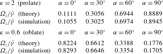
, as shown in table 1. For the mobility problem, we consider the free rotation of a spheroid in a shear flow,
 $\boldsymbol{U}^{\infty }=-\dot{\unicode[STIX]{x1D6FE}}y\boldsymbol{e}_{x}$
, where the revolution axis of the spheroid is on the shear plane (
 $z=0$
). We define
 $2\unicode[STIX]{x1D705}$
as the length of the axis of revolution scaled by the radius of a sphere with the same volume, and
 $\unicode[STIX]{x1D6FC}$
as the angle between the revolution axis and the
 $x$
-axis. We compute the instantaneous rotational velocity
 $\unicode[STIX]{x1D734}=\unicode[STIX]{x1D6FA}_{z}\boldsymbol{e}_{z}$
of the spheroid as a function of
 $\unicode[STIX]{x1D705}$
and
 $\unicode[STIX]{x1D6FC}$
, and validate the results against the analytical theory (Jeffery Reference Jeffery1922),
 $\unicode[STIX]{x1D6FA}_{z}/\dot{\unicode[STIX]{x1D6FE}}=0.5[1-(\unicode[STIX]{x1D705}^{3}-1)/(\unicode[STIX]{x1D705}^{3}+1)\cos 2\unicode[STIX]{x1D6FC}]$
. The comparison shown in table 2 shows a maximum discrepancy of below 1 %.
The non-dimensional hydrodynamic torque
 $\bar{T}_{z}=T_{z}/(\unicode[STIX]{x1D707}\unicode[STIX]{x1D714}L^{3})$
exerted on a single rod of varying slenderness
 $\unicode[STIX]{x1D716}$
which rotates about one of its ends at a prescribed rotational velocity
 $\unicode[STIX]{x1D714}$
in the
 $xy$
plane.

The non-dimensional rotational velocity
 $\unicode[STIX]{x1D6FA}_{z}/\dot{\unicode[STIX]{x1D6FE}}$
of a prolate (
 $\unicode[STIX]{x1D705}=2$
) and an oblate (
 $\unicode[STIX]{x1D705}=0.6$
) spheroid in shear flow
 $\boldsymbol{U}^{\infty }=-\dot{\unicode[STIX]{x1D6FE}}y\boldsymbol{e}_{x}$
as a function of the angle
 $\unicode[STIX]{x1D6FC}$
between its axis of revolution and the streamwise (
 $x$
) direction. The theoretical results are from Jeffery (Reference Jeffery1922).

4 Results: RF without hydrodynamic interactions
4.1 One individual rod:
 $N=1$

We first investigate one rod and plot its instantaneous rotational velocity
 $\bar{\unicode[STIX]{x1D714}}_{z}$
as a function of its orientation
 $\unicode[STIX]{x1D703}$
in figure 2(a). The off-centre displacement
 $\unicode[STIX]{x1D6FD}=1/8$
is fixed, and three characteristic channel widths
 $\unicode[STIX]{x1D70C}=2$
, 4 and 6 are studied. In the most confined case
 $\unicode[STIX]{x1D70C}=2$
, the RF results deviate with respect to the DNS data when
 $\unicode[STIX]{x1D703}=0$
, where the rod is oriented towards the nearest lateral wall; the relative difference between the two is approximately 24 %. This result is expected considering the rather strong confinement. When
 $\unicode[STIX]{x1D70C}=4$
and 6, the maximum discrepancy between the RF and DNS results is below 10 %. We thus conclude that the effect of this level of confinement can be neglected and will not be considered further.
(a) Instantaneous rotational velocity
 $\bar{\unicode[STIX]{x1D714}}_{z}$
of a single rod with an off-centre displacement
 $\unicode[STIX]{x1D6FD}=1/8$
in a channel flow. Empty and solid symbols denote, respectively, the results of resistive theory (RF) and DNS for three characteristic widths of flow
 $\unicode[STIX]{x1D70C}=2$
(circle),
 $\unicode[STIX]{x1D70C}=4$
(diamond) and
 $\unicode[STIX]{x1D70C}=6$
(square). The configurations of the rod corresponding to the fixed points
 $\unicode[STIX]{x1D703}_{f}=\unicode[STIX]{x03C0}/2$
and
 $\unicode[STIX]{x1D703}_{f}=3\unicode[STIX]{x03C0}/2$
are depicted in (b) and (c), respectively.

We can consider
 $\,\text{d}\unicode[STIX]{x1D703}/\text{d}\bar{t}=\bar{\unicode[STIX]{x1D714}}_{z}(\unicode[STIX]{x1D703})$
as a one-dimensional dynamical system and investigate the fixed points
 $\unicode[STIX]{x1D703}_{f}$
satisfying
 $\bar{\unicode[STIX]{x1D714}}_{z}(\unicode[STIX]{x1D703}_{f})=0$
and their stability. Noticing that
 $\unicode[STIX]{x1D6FD}+1\leqslant \unicode[STIX]{x1D70C}$
because the rod cannot penetrate the sidewalls and
 $\cos \unicode[STIX]{x1D703}\in [-1,1]$
, and using (3.8) we observe that
 $[6(\unicode[STIX]{x1D6FD}^{2}-\unicode[STIX]{x1D70C}^{2})+8\unicode[STIX]{x1D6FD}\cos \unicode[STIX]{x1D703}+3\cos ^{2}\unicode[STIX]{x1D703}]>0$
. Therefore,
 $\cos \unicode[STIX]{x1D703}_{f}=0$
leads to the two fixed points:
 $\unicode[STIX]{x1D703}_{f}=\unicode[STIX]{x03C0}/2$
, where the rod is aligned with the flow direction (figure 2
b), and
 $\unicode[STIX]{x1D703}_{f}=3\unicode[STIX]{x03C0}/2$
, where the rod is oriented opposite to the flow direction (figure 2
c). Their stability are dictated by the sign of the slope
 $\,\text{d}\bar{\unicode[STIX]{x1D714}}_{z}/\text{d}\unicode[STIX]{x1D703}|_{\unicode[STIX]{x1D703}_{f}}$
. We hence observe that the former/latter fixed point is stable/unstable because
 $\,\text{d}\bar{\unicode[STIX]{x1D714}}_{z}/\text{d}\unicode[STIX]{x1D703}|_{\unicode[STIX]{x1D703}_{f}=\unicode[STIX]{x03C0}/2}<0$
and
 $\,\text{d}\bar{\unicode[STIX]{x1D714}}_{z}/\text{d}\unicode[STIX]{x1D703}|_{\unicode[STIX]{x1D703}_{f}=3\unicode[STIX]{x03C0}/2}>0$
, as is also indicated in figure 2(a). We conclude that the watermill consisting of one rod will adopt a steady equilibrium position in the channel flow.
4.2 Two rods:
$N=2$

(a) Instantaneous rotational velocity
 $\bar{\unicode[STIX]{x1D714}}_{z}$
of a
 $N=2$
watermill with an off-centre displacement
 $\unicode[STIX]{x1D6FD}=1/8$
(diamond),
 $\unicode[STIX]{x1D6FD}=1/4$
(square) and
 $\unicode[STIX]{x1D6FD}=1/2$
(triangle) in a channel with a characteristic width
 $\unicode[STIX]{x1D70C}=5$
. Panels (b) and (c) indicate, respectively, the unstable (
 $\unicode[STIX]{x1D703}\rightarrow {\unicode[STIX]{x1D703}_{f}}^{-}$
) and stable (
 $\unicode[STIX]{x1D703}\rightarrow {\unicode[STIX]{x1D703}_{f}}^{+}$
) configurations of the half-stable fixed point
 $\unicode[STIX]{x1D703}_{f}=\unicode[STIX]{x03C0}/2$
.

We now consider a watermill consisting of two rods separated by
 $\unicode[STIX]{x03C0}$
, which of course is equivalent to a single rod of length
 $2L$
with its centre jointed at the rotation axis. The geometry has
 $2$
-fold rotational symmetry about the joint and hence its rotational velocity preserves the periodicity
 $\bar{\unicode[STIX]{x1D714}}_{z}(\unicode[STIX]{x1D703})=\bar{\unicode[STIX]{x1D714}}_{z}(\unicode[STIX]{x1D703}+\unicode[STIX]{x03C0})$
. Figure 3(a) shows
 $\bar{\unicode[STIX]{x1D714}}_{z}(\unicode[STIX]{x1D703})$
for
 $\unicode[STIX]{x1D703}\in [0,\unicode[STIX]{x03C0}]$
of the watermill displaced by three off-centre distances
 $\unicode[STIX]{x1D6FD}$
for a fixed channel width
 $\unicode[STIX]{x1D70C}=5$
. The rotational velocity reveals the mirror symmetry about
 $\unicode[STIX]{x1D703}=\unicode[STIX]{x03C0}/2$
. This result is indicated by the analytical expression equation (3.8) when
 $N=2$
, which also reflects the reversibility of the Stokes flow. The RF theory agrees reasonably well with the DNS data when the offset
 $\unicode[STIX]{x1D6FD}=1/4$
and
 $1/2$
; the
 $\unicode[STIX]{x1D703}$
-averaged relative difference between the theory and DNS is approximately 14 %. This difference, however, increases to 27 % for
 $\unicode[STIX]{x1D6FD}=1/8$
, because the absolute value of
 $\bar{\unicode[STIX]{x1D714}}_{z}$
becomes small and slight differences can introduce large relative deviations. It is worth noting that the slight asymmetry of the DNS data about
 $\unicode[STIX]{x1D703}=\unicode[STIX]{x03C0}/2$
reveals the role of weak confinement captured by the simulations.
By setting
 $\bar{\unicode[STIX]{x1D714}}_{z}(\unicode[STIX]{x1D703}_{f})=0$
, we identify the only fixed point
 $\unicode[STIX]{x1D703}_{f}=\unicode[STIX]{x03C0}/2$
representing the configuration when two rods are perfectly aligned with the flow direction. Since the slope
 $\,\text{d}\bar{\unicode[STIX]{x1D714}}_{z}/\text{d}\unicode[STIX]{x1D703}|_{\unicode[STIX]{x1D703}_{f}}=0$
, this fixed point is neither stable or unstable, but is regarded as half-stable (Strogatz Reference Strogatz2014), being unstable when
 $\unicode[STIX]{x1D703}\rightarrow {\unicode[STIX]{x1D703}_{f}}^{-}$
(positive slope) and stable when
 $\unicode[STIX]{x1D703}\rightarrow {\unicode[STIX]{x1D703}_{f}}^{+}$
(negative slope). The stability of this equilibrium position thus depends on the sign of perturbations: subject to a negative perturbation
 $\unicode[STIX]{x1D6FF}\unicode[STIX]{x1D703}<0$
, the system would rotate half a circle before it recovers to the equilibrium state (see figure 3
b); otherwise, it is immediately stabilised to the equilibrium state (see figure 3
c). In fact, this half-stability is in analogy with that of a prolate particle following Jeffery’s orbit in the shear plane when the particle’s axis of revolution is along the flow direction (Jeffery Reference Jeffery1922). The results imply that the two-rod watermill cannot be used in practice for flow manipulation on demand.
4.3 Three rods:
$N=3$

We present the RF-based rotational velocity
 $\bar{\unicode[STIX]{x1D714}}_{z}=-[16\unicode[STIX]{x1D6FD}+3\cos (3\unicode[STIX]{x1D703})]/16\unicode[STIX]{x1D70C}^{2}$
(see (3.8)) and its DNS counterpart in figure 4(a) for a three-rod watermill. The solution is characterised by the 3-fold rotational symmetry about the joint, so the rotation of the watermill satisfies the periodic condition
 $\bar{\unicode[STIX]{x1D714}}_{z}(\unicode[STIX]{x1D703})=\bar{\unicode[STIX]{x1D714}}_{z}(\unicode[STIX]{x1D703}+2\unicode[STIX]{x03C0}/3)$
. The agreement between the RF and DNS results is in general less favourable compared to the cases of
 $N=1$
and 2; the relative difference between them is approximately 23 %, 19 % and 20 % for
 $\unicode[STIX]{x1D6FD}=1/8$
,
 $1/4$
and
 $1/2$
, respectively. When
 $\unicode[STIX]{x1D6FD}=1/2$
, the magnitude of
 $\bar{\unicode[STIX]{x1D714}}_{z}$
is systematically underestimated by the RF theory. When
 $\unicode[STIX]{x1D6FD}=1/4$
or
 $1/2$
,
 $\bar{\unicode[STIX]{x1D714}}_{z}$
is negative regardless of the watermill orientation
 $\unicode[STIX]{x1D703}$
, so the watermill rotates continuously. However, when
 $\unicode[STIX]{x1D6FD}=1/8$
,
 $\bar{\unicode[STIX]{x1D714}}_{z}$
is positive only as
 $\unicode[STIX]{x1D703}$
is close to
 $\unicode[STIX]{x03C0}/3$
. In fact, the analytical expression indeed indicates that the fixed-point solutions satisfying
 $\cos (3\unicode[STIX]{x1D703})=-16\unicode[STIX]{x1D6FD}/3$
appear when
 $\unicode[STIX]{x1D6FD}$
is less than or equal to a critical value
 $\unicode[STIX]{x1D6FD}_{\ast }=3/16$
; otherwise when
 $\unicode[STIX]{x1D6FD}>\unicode[STIX]{x1D6FD}_{\ast }$
,
 $\bar{\unicode[STIX]{x1D714}}_{z}(\unicode[STIX]{x1D703})<0$
for any
 $\unicode[STIX]{x1D703}$
. In the former case, we can identify only one fixed point
 $\unicode[STIX]{x1D703}_{f}=[2\unicode[STIX]{x03C0}-\arccos (-16\unicode[STIX]{x1D6FD}/3)]/3$
and it is stable. The DNS results for
 $\bar{\unicode[STIX]{x1D714}}_{z}$
reach their maximum when
 $\unicode[STIX]{x1D703}=\unicode[STIX]{x03C0}/3$
, which is consistent with the RF prediction. In figure 4(b), we plot
 $\bar{\unicode[STIX]{x1D714}}_{z}|_{\unicode[STIX]{x1D703}=\unicode[STIX]{x03C0}/3}$
given by DNS as a function of the offset
 $\unicode[STIX]{x1D6FD}$
. The results show that the critical offset is slightly above
 $1/8$
, qualitatively confirming the theoretical prediction
 $\unicode[STIX]{x1D6FD}_{\ast }=3/16$
. We conclude that in order to continuously rotate, a three-rod watermill needs to be placed a critical distance away from the flow centre.
(a) Instantaneous rotational velocity
 $\bar{\unicode[STIX]{x1D714}}_{z}$
of a
 $N=3$
watermill with an off-centre displacement
 $\unicode[STIX]{x1D6FD}=1/8$
(diamond),
 $\unicode[STIX]{x1D6FD}=1/4$
(square) and
 $\unicode[STIX]{x1D6FD}=1/2$
(triangle) in a channel flow of a characteristic width
 $\unicode[STIX]{x1D70C}=5$
. (b) DNS results of
 $\bar{\unicode[STIX]{x1D714}}_{z}$
versus
 $\unicode[STIX]{x1D6FD}$
for a fixed orientation
 $\unicode[STIX]{x1D703}=\unicode[STIX]{x03C0}/3$
.

4.4 More than three rods:
$N\geqslant 4$

Instantaneous rotational velocity
 $\bar{\unicode[STIX]{x1D714}}_{z}$
of a watermill with an off-centre displacement (a)
 $\unicode[STIX]{x1D6FD}=0.1$
, (b)
 $\unicode[STIX]{x1D6FD}=1/2$
and (c)
 $\unicode[STIX]{x1D6FD}=1$
in a channel with a characteristic width
 $\unicode[STIX]{x1D70C}=5$
. The horizontal dashed line corresponds to the RF prediction
 $\bar{\unicode[STIX]{x1D714}}_{z}=-\unicode[STIX]{x1D6FD}/\unicode[STIX]{x1D70C}^{2}$
and the symbols represent the orientation-discrete DNS results for the watermill consisting of
 $N=4$
(cross), 5 (square), 6 (star), 7 (diamond), 8 (circle) and 9 (triangle) rods.

An important observation from the simple RF theory is that as long as
 $N\geqslant 4$
, the rotational velocity of the watermill
 $\bar{\unicode[STIX]{x1D714}}_{z}=-\unicode[STIX]{x1D6FD}/\unicode[STIX]{x1D70C}^{2}$
is independent of
 $N$
or its orientation
 $\unicode[STIX]{x1D703}$
(see (3.8)). This striking independence stems from the torque calculation that involves linear combinations of
 $\cos \unicode[STIX]{x1D703}$
,
 $\cos 2\unicode[STIX]{x1D703}$
and
 $\cos 3\unicode[STIX]{x1D703}$
, as indicated by (3.7), which is the mathematical reason that leads to the
 $N\geqslant 4$
threshold for a rotation speed independent of
 $N$
(see appendix A for the details). This prediction is qualitatively confirmed by the comparison between the RF and DNS data in figure 5 for
 $N\in [4,9]$
with three off-centre distances
 $\unicode[STIX]{x1D6FD}=0.1$
,
 $1/2$
and 1. Due to the periodicity of
 $\bar{\unicode[STIX]{x1D714}}_{z}$
in
 $\unicode[STIX]{x1D703}$
, as demonstrated in the previous sections, the rotational velocity is plotted versus
 $\unicode[STIX]{x1D703}/\unicode[STIX]{x1D719}$
to ease the comparison between different
 $N$
. Figure 5 shows that the RF results agree with the numerical data qualitatively. Compared to the independence of
 $\bar{\unicode[STIX]{x1D714}}_{z}$
on
 $\unicode[STIX]{x1D703}$
predicted by RF, the DNS suggests that
 $\bar{\unicode[STIX]{x1D714}}_{z}$
exhibits a weak dependence on the orientation
 $\unicode[STIX]{x1D703}$
at
 $\unicode[STIX]{x1D6FD}=0.1$
while its variation in
 $\unicode[STIX]{x1D703}$
is negligible at
 $\unicode[STIX]{x1D6FD}=1/2$
and 1. We also observe that the RF theory underestimates
 $\bar{\unicode[STIX]{x1D714}}_{z}$
systematically compared to the DNS data, resulting in a relative difference of approximately 30 %. Another important observation is that the magnitude of
 $\bar{\unicode[STIX]{x1D714}}_{z}$
increases in general with the number
 $N$
of rods.
We infer that the underestimation of RF theory might be attributed to its lack of accounting for the inter-rod hydrodynamic interactions, which promotes the rotation of the watermill. Intuitively, the hydrodynamic interactions depend significantly on the separation distance (indicated by
 $\unicode[STIX]{x1D719}$
) between every two successive rods, and hence it should become stronger with decreasing
 $\unicode[STIX]{x1D719}$
(increasing
 $N$
). This intuition might also explain the positive relation between
 $\bar{\unicode[STIX]{x1D714}}_{z}$
and
 $N$
that is unaccounted for by the RF theory. We address these ideas further in the next section.
5 RF considering hydrodynamic interactions
5.1 Theoretical framework
The above results suggest that there are configurations where it is important to take hydrodynamic interactions into account in order to provide a more accurate prediction of the rotational velocities than the classical RF theory. As far as we know, theoretical efforts have been reported to address the hydrodynamic interactions between a slender body and a wall (Mestre Reference Mestre1973; Russel et al.
Reference Russel, Hinch, Leal and Tieffenbruck1977; Barta & Liron Reference Barta and Liron1988) or two walls (Katz Reference Katz1974). Based on the classical RF theory, we hereby make an attempt by utilising a theoretical framework which Man et al. (Reference Man, Koens and Lauga2016) recently developed for two interacting weakly deformable filaments that are in parallel in their relaxed state (see figure 6
a). As a first step, we will consider a simplified configuration rather than the original set-up, focusing on two or three rods, i.e.
 $N\leqslant 3$
; further, the separation angle
 $\unicode[STIX]{x1D719}$
is independent of
 $N$
and is tuned arbitrarily to be much smaller than
 $2\unicode[STIX]{x03C0}/N$
, in contrast to the value
 $\unicode[STIX]{x1D719}=2\unicode[STIX]{x03C0}/N$
of the original set-up.
Sketch of two interacting rods/filaments. (a) The configuration of two filaments studied by Man et al. (Reference Man, Koens and Lauga2016), where the dashed lines denote their initial, undeformed states. The rods are aligned (b) in the
 $\boldsymbol{e}_{bi}=\boldsymbol{e}_{y}$
direction and (c) in an arbitrary direction
 $\boldsymbol{e}_{bi}=\cos \unicode[STIX]{x1D703}\boldsymbol{e}_{x}+\sin \unicode[STIX]{x1D703}\boldsymbol{e}_{y}$
; the dashed arrow indicates the internal bisector of the two rods. (d) The configuration of three rods.

We start with a two-rod watermill and consider the limit that
 $\unicode[STIX]{x1D716}\ll \unicode[STIX]{x1D719}\ll 1$
(see figure 6
b,c). This limit indicates first that the two rods are approximately parallel, viz.
 $\boldsymbol{t}^{(1)}\approx \boldsymbol{t}^{(2)}\approx \boldsymbol{e}_{bi}$
, where
 $\boldsymbol{e}_{bi}$
is the orientation of their internal bisector; second, their typical separation distance
 $h\sim L\unicode[STIX]{x1D719}$
is much smaller than
 $L$
but much larger than the radius
 $a$
, namely
 $a\ll h\ll L$
. Note that in the near-hinge segment with sufficiently small arclength
 $s\leqslant a$
, the latter approximation is violated. However, the introduced errors of computing the corresponding hydrodynamic torque is rather limited, because of the very small prefactor, namely the distance
 $s$
away from the hinge.
The hydrodynamic force per unit length
 $\boldsymbol{f}^{(k)}$
exerted by the fluid on the two rods is
 $$\begin{eqnarray}\displaystyle & \displaystyle \boldsymbol{f}^{(1)}-\unicode[STIX]{x1D645}^{(1)}\boldsymbol{\cdot }\boldsymbol{v}^{(2)\rightarrow (1)}=-\unicode[STIX]{x1D645}^{(1)}\boldsymbol{\cdot }\left[\frac{\unicode[STIX]{x2202}\boldsymbol{r}^{(1)}}{\unicode[STIX]{x2202}t}-\boldsymbol{U}^{\infty }(\boldsymbol{r}^{(1)})\right], & \displaystyle\end{eqnarray}$$
 $$\begin{eqnarray}\displaystyle & \displaystyle \boldsymbol{f}^{(2)}-\unicode[STIX]{x1D645}^{(2)}\boldsymbol{\cdot }\boldsymbol{v}^{(1)\rightarrow (2)}=-\unicode[STIX]{x1D645}^{(2)}\boldsymbol{\cdot }\left[\frac{\unicode[STIX]{x2202}\boldsymbol{r}^{(2)}}{\unicode[STIX]{x2202}t}-\boldsymbol{U}^{\infty }(\boldsymbol{r}^{(2)})\right], & \displaystyle\end{eqnarray}$$
 $\boldsymbol{v}^{(2)\rightarrow (1)}$
denotes the velocity induced by the second rod on the first rod. Following Man et al. (Reference Man, Koens and Lauga2016), we first assume that the orientation of the two rods
 $\boldsymbol{e}_{bi}$
is parallel with
 $\boldsymbol{e}_{y}$
(see figure 6
b). The induced velocity
 $\boldsymbol{v}^{(2)\rightarrow (1)}$
can be integrated asymptotically in the limit of
 $a\ll h\ll L$
(Man et al.
Reference Man, Koens and Lauga2016),
 $$\begin{eqnarray}\displaystyle \boldsymbol{v}^{(2)\rightarrow (1)}=\frac{1}{4\unicode[STIX]{x03C0}\unicode[STIX]{x1D707}}\ln \left(\frac{h(s)}{L}\right)(\unicode[STIX]{x1D644}+\boldsymbol{e}_{y}\boldsymbol{e}_{y})\boldsymbol{\cdot }\boldsymbol{f}^{(2)}(s), & & \displaystyle\end{eqnarray}$$
where
 $\boldsymbol{h}(s)=\boldsymbol{r}^{(1)}(s)-\boldsymbol{r}^{(2)}(s)$
denotes the local displacement vector between the two points
 $\boldsymbol{r}^{(1)}(s)$
and
 $\boldsymbol{r}^{(2)}(s)$
on the rods’ centrelines, and
 $h(s)=|\boldsymbol{h}(s)|=2s\,\text{sin}(\unicode[STIX]{x1D719}/2)$
. We will retain the functional form with the sine, so as to possibly see whether this approach might work for large
 $\unicode[STIX]{x1D719}$
values, though recognise that the self-consistency for small
 $\unicode[STIX]{x1D719}$
implies
 $\sin (\unicode[STIX]{x1D719}/2)\sim \unicode[STIX]{x1D719}/2$
.
Because
 $\boldsymbol{t}^{(1)}\approx \boldsymbol{t}^{(2)}\approx \boldsymbol{e}_{y}$
, we obtain
 $\unicode[STIX]{x1D645}^{(1)}(\boldsymbol{t}^{(1)})\approx \unicode[STIX]{x1D645}^{(2)}(\boldsymbol{t}^{(2)})\approx \unicode[STIX]{x1D645}(\boldsymbol{e}_{y})=\unicode[STIX]{x1D709}_{\bot }(\unicode[STIX]{x1D644}-\boldsymbol{e}_{y}\boldsymbol{e}_{y}/2)$
. Thus, the force density involving the induced velocity can be reformulated as
 $$\begin{eqnarray}\displaystyle -\unicode[STIX]{x1D645}^{(1)}\boldsymbol{\cdot }\boldsymbol{v}^{(2)\rightarrow (1)}=\unicode[STIX]{x1D706}(s)\boldsymbol{f}^{(2)}, & & \displaystyle\end{eqnarray}$$
where
 $\unicode[STIX]{x1D706}(s)=\ln (h(s)/L)/\ln \unicode[STIX]{x1D716}$
. An important observation is that (5.3) does not depend on the orientation
 $\boldsymbol{e}_{bi}$
of the two rods. Because of this independence from
 $\boldsymbol{e}_{bi}$
, by considering a general orientation
 $\boldsymbol{e}_{bi}=\cos \unicode[STIX]{x1D703}\boldsymbol{e}_{x}+\sin \unicode[STIX]{x1D703}\boldsymbol{e}_{y}$
(see figure 6
c), we can always rewrite (5.1) and obtain a linear system with its left-hand side independent of
 $\unicode[STIX]{x1D703}$
as
 $$\begin{eqnarray}\displaystyle & \displaystyle \boldsymbol{f}^{(1)}+\unicode[STIX]{x1D706}(s)\boldsymbol{f}^{(2)}=-\unicode[STIX]{x1D645}^{(1)}\boldsymbol{\cdot }\left[\frac{\unicode[STIX]{x2202}\boldsymbol{r}^{(1)}}{\unicode[STIX]{x2202}t}-\boldsymbol{U}^{\infty }(\boldsymbol{r}^{(1)})\right], & \displaystyle\end{eqnarray}$$
 $$\begin{eqnarray}\displaystyle & \displaystyle \boldsymbol{f}^{(2)}+\unicode[STIX]{x1D706}(s)\boldsymbol{f}^{(1)}=-\unicode[STIX]{x1D645}^{(2)}\boldsymbol{\cdot }\left[\frac{\unicode[STIX]{x2202}\boldsymbol{r}^{(2)}}{\unicode[STIX]{x2202}t}-\boldsymbol{U}^{\infty }(\boldsymbol{r}^{(2)})\right]. & \displaystyle\end{eqnarray}$$
We note that (5.4) is slightly different from equation (25) of Man et al. (Reference Man, Koens and Lauga2016). In their work, they aimed to model two flexible filaments initially undeformed and oriented parallel to the
 $\boldsymbol{e}_{y}$
direction (see figure 6
a). Once deformed, they become slightly misaligned, and
 $\boldsymbol{t}^{(k)}(s)$
and
 $\unicode[STIX]{x1D645}^{(k)}(\boldsymbol{t}^{(k)}(s))$
, with
 $k=1,2$
, on their centrelines, both vary with the arclength
 $s$
. Adopting the long-wavelength approximation,
 $\unicode[STIX]{x1D645}^{(k)}\approx \unicode[STIX]{x1D645}^{(k)}(\boldsymbol{e}_{y})$
is assumed; that said, they took the initial direction
 $\boldsymbol{e}_{y}$
of the filaments to approximately calculate
 $\unicode[STIX]{x1D645}^{(k)}$
, neglecting the influence of deformation. Similar to Man et al. (Reference Man, Koens and Lauga2016), we compute
 $\unicode[STIX]{x1D645}^{(k)}$
on the left-hand side of (5.1) based on
 $\boldsymbol{e}_{bi}$
, the approximate orientation of the two rods, hence we have
 $\unicode[STIX]{x1D645}^{(k)}\approx \unicode[STIX]{x1D645}^{(k)}(\boldsymbol{e}_{bi})$
. This step facilitates the expression of
 $-\unicode[STIX]{x1D645}^{(k)}\boldsymbol{\cdot }\boldsymbol{v}^{(j)\rightarrow (k)}$
as a function of local force density
 $\boldsymbol{f}^{(j)}$
, with
 $k\neq j$
. Therefore, maintaining generality in geometry, the orientations of our rigid rods
 $\boldsymbol{t}^{(k)}$
are well defined as
 $$\begin{eqnarray}\displaystyle \left.\begin{array}{@{}c@{}}\boldsymbol{t}^{(1)}=\cos \left(\unicode[STIX]{x1D703}-\unicode[STIX]{x1D719}/2\right)\boldsymbol{e}_{x}+\sin \left(\unicode[STIX]{x1D703}-\unicode[STIX]{x1D719}/2\right)\boldsymbol{e}_{y},\\ \boldsymbol{t}^{(2)}=\cos \left(\unicode[STIX]{x1D703}+\unicode[STIX]{x1D719}/2\right)\boldsymbol{e}_{x}+\sin \left(\unicode[STIX]{x1D703}+\unicode[STIX]{x1D719}/2\right)\boldsymbol{e}_{y},\end{array}\right\} & & \displaystyle\end{eqnarray}$$
which are used to compute
 $\unicode[STIX]{x1D645}^{(k)}(\boldsymbol{t}^{(k)})$
on the right-hand side of (5.1). These steps lead to a discrepancy in computing
 $\unicode[STIX]{x1D645}^{(k)}$
on the left- and right-hand sides of (5.1), which vanishes asymptotically when
 $\unicode[STIX]{x1D719}\rightarrow 0$
. In the small-
 $\unicode[STIX]{x1D719}$
limit, our derivations are consistent.
By inverting the matrix of equation (5.4), we obtain the force density
 $\boldsymbol{f}^{(k)}$
 $$\begin{eqnarray}\displaystyle \boldsymbol{f}^{(k)}(s) & = & \displaystyle -\frac{1}{1-\unicode[STIX]{x1D706}^{2}(s)}\left(\unicode[STIX]{x1D645}^{(k)}\boldsymbol{\cdot }\left[\frac{\unicode[STIX]{x2202}\boldsymbol{r}^{(k)}}{\unicode[STIX]{x2202}t}-\boldsymbol{U}^{\infty }(\boldsymbol{r}^{(k)})\right]-\unicode[STIX]{x1D706}(s)\unicode[STIX]{x1D645}^{(j)}\boldsymbol{\cdot }\left[\frac{\unicode[STIX]{x2202}\boldsymbol{r}^{(j)}}{\unicode[STIX]{x2202}t}-\boldsymbol{U}^{\infty }(\boldsymbol{r}^{(j)})\right]\right),\nonumber\\ \displaystyle & & \displaystyle \quad k\neq j.\end{eqnarray}$$
The above approach has been extended to the case of three rods (see figure 6 d). By considering the mutual hydrodynamic interactions between every pair of two rods, we obtain the linear system as
 $$\begin{eqnarray}\displaystyle & \displaystyle \boldsymbol{f}^{(1)}+\unicode[STIX]{x1D706}(s)\boldsymbol{f}^{(2)}+\unicode[STIX]{x1D6EC}(s)\boldsymbol{f}^{(3)}=-\unicode[STIX]{x1D645}^{(1)}\boldsymbol{\cdot }\left[\frac{\unicode[STIX]{x2202}\boldsymbol{r}^{(1)}}{\unicode[STIX]{x2202}t}-\boldsymbol{U}^{\infty }(\boldsymbol{r}^{(1)})\right], & \displaystyle\end{eqnarray}$$
 $$\begin{eqnarray}\displaystyle & \displaystyle \boldsymbol{f}^{(2)}+\unicode[STIX]{x1D706}(s)(\,\boldsymbol{f}^{(1)}+\boldsymbol{f}^{(3)})=-\unicode[STIX]{x1D645}^{(2)}\boldsymbol{\cdot }\left[\frac{\unicode[STIX]{x2202}\boldsymbol{r}^{(2)}}{\unicode[STIX]{x2202}t}-\boldsymbol{U}^{\infty }(\boldsymbol{r}^{(2)})\right], & \displaystyle\end{eqnarray}$$
 $$\begin{eqnarray}\displaystyle & \displaystyle \boldsymbol{f}^{(3)}+\unicode[STIX]{x1D706}(s)\boldsymbol{f}^{(2)}+\unicode[STIX]{x1D6EC}(s)\boldsymbol{f}^{(1)}=-\unicode[STIX]{x1D645}^{(3)}\boldsymbol{\cdot }\left[\frac{\unicode[STIX]{x2202}\boldsymbol{r}^{(3)}}{\unicode[STIX]{x2202}t}-\boldsymbol{U}^{\infty }(\boldsymbol{r}^{(3)})\right], & \displaystyle\end{eqnarray}$$
 $\unicode[STIX]{x1D6EC}(s)=\ln (H(s)/L)/\ln \unicode[STIX]{x1D716}$
, and
 $H(s)=2s\sin \unicode[STIX]{x1D719}$
denotes the distance between the centreline points
 $\boldsymbol{r}^{(1)}(s)$
and
 $\boldsymbol{r}^{(3)}(s)$
of the first rod and third rod separated by
 $2\unicode[STIX]{x1D719}$
. Abbreviating
 $\unicode[STIX]{x1D645}^{(k)}\boldsymbol{\cdot }[\unicode[STIX]{x2202}\boldsymbol{r}^{(k)}/\unicode[STIX]{x2202}t-\boldsymbol{U}^{\infty }(\boldsymbol{r}^{(k)})]$
by
 $\boldsymbol{R}^{(k)}$
, we obtain the force densities as
 $$\begin{eqnarray}\displaystyle & \displaystyle \boldsymbol{f}^{(1)}=\frac{(1-\unicode[STIX]{x1D706}^{2})\boldsymbol{R}^{(1)}+\unicode[STIX]{x1D706}(\unicode[STIX]{x1D6EC}-1)\boldsymbol{R}^{(2)}+(\unicode[STIX]{x1D706}^{2}-\unicode[STIX]{x1D6EC})\boldsymbol{R}^{(3)}}{(1-\unicode[STIX]{x1D6EC})(2\unicode[STIX]{x1D706}^{2}-\unicode[STIX]{x1D6EC}-1)}, & \displaystyle\end{eqnarray}$$
 $$\begin{eqnarray}\displaystyle & \displaystyle \boldsymbol{f}^{(2)}=\frac{(\unicode[STIX]{x1D6EC}+1)\boldsymbol{R}^{(2)}-\unicode[STIX]{x1D706}(\boldsymbol{R}^{(1)}+\boldsymbol{R}^{(3)})}{2\unicode[STIX]{x1D706}^{2}-\unicode[STIX]{x1D6EC}-1}, & \displaystyle\end{eqnarray}$$
 $$\begin{eqnarray}\displaystyle & \displaystyle \boldsymbol{f}^{(3)}=\frac{(\unicode[STIX]{x1D706}^{2}-\unicode[STIX]{x1D6EC})\boldsymbol{R}^{(1)}+\unicode[STIX]{x1D706}(\unicode[STIX]{x1D6EC}-1)\boldsymbol{R}^{(2)}+(1-\unicode[STIX]{x1D706}^{2})\boldsymbol{R}^{(3)}}{(1-\unicode[STIX]{x1D6EC})(2\unicode[STIX]{x1D706}^{2}-\unicode[STIX]{x1D6EC}-1)}. & \displaystyle\end{eqnarray}$$
5.2 Results: resistance problems
We start with the resistance problems. We consider a quiescent environment, where two or three rods rotate in the
 $xy$
plane about the joint at a prescribed rotational velocity
 $\unicode[STIX]{x1D714}$
. The non-dimensional hydrodynamic torque
 $T_{z}/(\unicode[STIX]{x1D707}\unicode[STIX]{x1D714}L^{3})$
exerted on one rod is computed by RF, RF-HI theory and DNS, and shown in figure 7. For two rods (figure 7
a), we observe that when they get closer to each other, i.e.
 $\unicode[STIX]{x1D719}$
decreases, the torque calculated by DNS decreases significantly. This implies the role of hydrodynamic interactions to reduce the hydrodynamic resistances. The RF theory cannot predict any hydrodynamic interactions, while the RF-HI predictions agree with the DNS data very well when
 $\unicode[STIX]{x1D719}\leqslant \unicode[STIX]{x03C0}/24$
. At the smallest separation angle,
 $\unicode[STIX]{x1D719}=\unicode[STIX]{x03C0}/36$
, the relative errors of the RF and RF-HI predictions are 68 % and 0.3 %, respectively. Increasing
 $\unicode[STIX]{x1D719}$
, the RF-HI theory deviates from the DNS data, which is expected considering the
 $\unicode[STIX]{x1D719}\rightarrow 0$
asymptotic limit in which the RF-HI theory is derived. When
 $\unicode[STIX]{x1D719}=\unicode[STIX]{x03C0}/3$
, the relative errors of the RF and RF-HI predictions are 11 % and 8 %; the RF-HI theory fails to improve the prediction significantly.
In the case of three rods (figure 7
b), the DNS data shows that the torque on the middle rod is less than that on the side rods because the middle rod experiences stronger hydrodynamic interactions than the other two. The RF-HI theory predicts the hydrodynamic interactions well when
 $\unicode[STIX]{x1D719}\leqslant \unicode[STIX]{x03C0}/12$
. For example, for the side rod, when
 $\unicode[STIX]{x1D719}=\unicode[STIX]{x03C0}/36$
, the relative error is 87 % for the RF prediction, which drops to 2 % for the RF-HI prediction; when
 $\unicode[STIX]{x1D719}=\unicode[STIX]{x03C0}/3$
, the errors for the two are 15 % and 6 %, respectively.
Non-dimensional hydrodynamic torque
 $T_{z}/(\unicode[STIX]{x1D707}\unicode[STIX]{x1D714}L^{3})$
exerted on a single rod of a (a) two-rod and (b) three-rod watermill rotating in the
 $xy$
plane at a prescribed velocity
 $\unicode[STIX]{x1D714}$
. The torques computed by RF, RF-HI theory and DNS are shown versus the separation angle
 $\unicode[STIX]{x1D719}$
. For three rods, solid/hollow symbols indicate the torques on the middle/side rod.

The instantaneous non-dimensional rotational velocity
 $|\unicode[STIX]{x1D714}_{z}|/\dot{\unicode[STIX]{x1D6FE}}$
of a shear-driven two-rod watermill oriented at (a)
 $\unicode[STIX]{x1D703}=0$
and (b)
 $\unicode[STIX]{x1D703}=\unicode[STIX]{x03C0}/2$
, as a function of the separation angle
 $\unicode[STIX]{x1D719}$
. The DNS data, RF-HI and RF predictions are compared.

The instantaneous non-dimensional rotational velocity
 $|\unicode[STIX]{x1D714}_{z}|/\dot{\unicode[STIX]{x1D6FE}}$
of a shear-driven three-rod watermill oriented at (a)
 $\unicode[STIX]{x1D703}=0$
and (b)
 $\unicode[STIX]{x1D703}=\unicode[STIX]{x03C0}/2$
, as a function of the separation angle
 $\unicode[STIX]{x1D719}$
. The DNS data, RF-HI and RF predictions are compared.

5.3 Results: mobility problems
Having demonstrated the resistance problems, we next address the mobility problems. Namely, for a freely rotating two/three-rod watermill subject to an ambient shear flow
 $\boldsymbol{U}^{\infty }=\dot{\unicode[STIX]{x1D6FE}}y\boldsymbol{e}_{x}$
, where
 $\dot{\unicode[STIX]{x1D6FE}}$
is the shear rate, we solve for its rotational velocity
 $\unicode[STIX]{x1D714}_{z}$
based on the condition that the total hydrodynamic torque exerted on the watermill is zero. The rotation of the watermill depends on its orientation,
 $\unicode[STIX]{x1D703}$
, defined here as the angle between the bisector of the two rods when
 $N=2$
or the middle rod when
 $N=3$
with respect to the
 $x$
-axis (see figure 6
c,d). For two orientations
 $\unicode[STIX]{x1D703}=0$
and
 $\unicode[STIX]{x03C0}/2$
, the non-dimensional rotational velocities
 $\unicode[STIX]{x1D714}_{z}/\dot{\unicode[STIX]{x1D6FE}}$
versus the separation angle
 $\unicode[STIX]{x1D719}$
are shown in figure 8 for
 $N=2$
and figure 9 for
 $N=3$
. As expected from familiarity with the Jeffery orbit of a rigid rod subject to a shear flow (Jeffery Reference Jeffery1922), in both cases, the watermill rotates faster when it is aligned with the shear direction (
 $\unicode[STIX]{x1D703}=\unicode[STIX]{x03C0}/2$
) than when it is aligned with the flow direction (
 $\unicode[STIX]{x1D703}=0$
). This feature can be explained by decomposing the shear flow by a clockwise rotational flow and a planar hyperbolic flow that stretches (respectively compresses) fluid elements in the
 $x=y$
(respectively
 $x=-y$
) direction. Indeed, Jeffery (Reference Jeffery1922) determined that a single rod under shear attained its maximum rotational velocity
 $|\unicode[STIX]{x1D714}_{z}|=\dot{\unicode[STIX]{x1D6FE}}$
at
 $\unicode[STIX]{x1D703}=\unicode[STIX]{x03C0}/2$
and minimum
 $|\unicode[STIX]{x1D714}_{z}|=0$
at
 $\unicode[STIX]{x1D703}=0$
. Figure 8 shows that in the
 $\unicode[STIX]{x1D719}\rightarrow 0$
limit, the two rods merge to one whose rotational velocity indeed approaches these two extremes. With increasing
 $\unicode[STIX]{x1D719}$
, the two rods located at
 $\unicode[STIX]{x1D703}=0$
begin to move away from the low-rotation region and hence
 $|\unicode[STIX]{x1D714}_{z}|$
increases with
 $\unicode[STIX]{x1D719}$
; its decrease with
 $\unicode[STIX]{x1D719}$
when they are located at
 $\unicode[STIX]{x1D703}=\unicode[STIX]{x03C0}/2$
can be explained likewise. The RF theory deviates with the DNS data considerably for all of the
 $\unicode[STIX]{x1D719}$
values, while the RF-HI theory agrees with the DNS data when
 $\unicode[STIX]{x1D719}\leqslant \unicode[STIX]{x03C0}/24$
but otherwise exhibits limited improvement over the RF theory. More specifically, when
 $\unicode[STIX]{x1D703}=0$
, the relative errors of the RF and RF-HI predictions for
 $\unicode[STIX]{x1D719}=\unicode[STIX]{x03C0}/36$
are 78 % and 0.5 %, respectively; they become 34 % and 24 % for
 $\unicode[STIX]{x1D719}=\unicode[STIX]{x03C0}/4$
. The physical picture for
 $N=3$
presented in figure 9 resembles that of
 $N=2$
; a notable difference is that the agreement between the RF-HI theory and DNS data has improved, which does not degrade significantly with
 $\unicode[STIX]{x1D719}$
until
 $\unicode[STIX]{x1D719}\geqslant 5\unicode[STIX]{x03C0}/24$
.
We finally present in figure 10 the rotational velocities
 $\bar{\unicode[STIX]{x1D714}}_{z}$
versus
 $\unicode[STIX]{x1D719}$
of a two-rod watermill oriented at (a)
 $\unicode[STIX]{x1D703}=0$
, (b)
 $\unicode[STIX]{x1D703}=\unicode[STIX]{x03C0}/3$
and (c)
 $\unicode[STIX]{x1D703}=5\unicode[STIX]{x03C0}/6$
in a channel flow with a characteristic width
 $\unicode[STIX]{x1D70C}=5$
and off-centre displacement
 $\unicode[STIX]{x1D6FD}=1$
. For all the orientations, the magnitude of
 $\bar{\unicode[STIX]{x1D714}}_{z}$
increases with decreasing
 $\unicode[STIX]{x1D719}$
. Both the RF and RF-HI theories predict such a trend and agree with the DNS data: when
 $\unicode[STIX]{x1D703}=0$
, the relative errors of the RF and RF-HI predictions for
 $\unicode[STIX]{x1D719}=\unicode[STIX]{x03C0}/36$
are 15 % and 11 %, respectively; they are 19 % and 13 % for
 $\unicode[STIX]{x1D719}=\unicode[STIX]{x03C0}/4$
. Overall, the RF-HI theory makes a limited improvement over the RF counterpart. The results of a three-rod watermill are similar to this two-rod case and hence are not reported here.
Similar to the set-up in figure 8, but subject to a channel flow (instead of shear flow) with a characteristic width
 $\unicode[STIX]{x1D70C}=5$
and off-centre displacement
 $\unicode[STIX]{x1D6FD}=1$
, where the watermill is oriented at (a)
 $\unicode[STIX]{x1D703}=0$
, (b)
 $\unicode[STIX]{x1D703}=\unicode[STIX]{x03C0}/3$
and (c)
 $\unicode[STIX]{x1D703}=5\unicode[STIX]{x03C0}/6$
.

6 Conclusions and discussions
Electrically or magnetically driven rotary components are commonly applied in microfluidic devices for pumping and mixing. In this work, we have performed a theoretical and computational study on the hydrodynamics of an anchored watermill as a model passive rotary microfluidic element whose motion is created by the flow. This idea was already studied for configurations with a freely rotating cylinder in a flow (Day & Stone Reference Day and Stone2000). Our work for a watermill configuration is motivated by the recent experiments of Moon et al. (Reference Moon, Tsai and Hwang2015), which utilised the underlying flow alone to rotate microgears in a microfluidic channel.
We model the watermill as a collection of slender cylindrical rods (like paddles) jointed on a common end, focusing on its hydrodynamic behaviour in an unbounded low-Reynolds-number, pressure-driven flow. The classical RF theory linking the hydrodynamic forces on the rods and their velocities is used to find the relation between the hydrodynamic torque on the watermill and its rotational velocity. By employing the torque-free condition of the flow-rotated watermill, we obtain the rotational velocities as a function of the number
 $N$
of rods, the off-centre displacement
 $\unicode[STIX]{x1D6FD}$
and orientation
 $\unicode[STIX]{x1D703}$
of the watermill, and the characteristic width
 $\unicode[STIX]{x1D70C}$
of the channel flow. For
 $N\leqslant 3$
, the rotational velocity
 $\bar{\unicode[STIX]{x1D714}}_{z}(\unicode[STIX]{x1D703})=\,\text{d}\unicode[STIX]{x1D703}/\text{d}\bar{t}$
of the watermill is a function of its orientation
 $\unicode[STIX]{x1D703}$
. By regarding
 $\bar{\unicode[STIX]{x1D714}}_{z}(\unicode[STIX]{x1D703})$
as a one-dimensional dynamical system, we have analysed its fixed points (indicating the equilibrium orientations of the watermill) and their stability. For
 $N=1$
, the single-rod watermill will adopt a stable equilibrium orientation that is aligned with the downstream flow direction. For
 $N=2$
, one half-stable fixed-point solution emerges, corresponding to the configuration in which the two-rod watermill is parallel with the underlying flow. For
 $N=3$
, when it is placed close enough to the centre of the flow, the watermill is aligned with a stable equilibrium orientation; otherwise it keeps rotating in flow, implying the absence of fixed points when
 $\unicode[STIX]{x1D6FD}$
is above a critical value. More interestingly, when
 $N\geqslant 4$
, the rotational velocity
 $\bar{\unicode[STIX]{x1D714}}_{z}=-\unicode[STIX]{x1D6FD}/\unicode[STIX]{x1D70C}^{2}$
is independent of
 $N$
and
 $\unicode[STIX]{x1D703}$
. Namely, the watermill is able to rotate at a constant velocity as long as it is not exactly on the centreline of the Poiseuille flow. To the best of our knowledge, this striking independence has not been reported by the previous studies. We believe that these results will provide a fundamental yet practical guide for the future experimental implementation of such flow-driven rotary devices.
It is worth pointing that the independence of the rotational velocity predicted by the RF theory reveals the full rotational symmetry (that is of infinite order) as long as the geometry of the watermill exhibits a rotational symmetry of at least order four; see (3.8). We note that a referee pointed out this observation exemplifies how a lower-fold symmetry may lead to a subtle unexpectedly higher-fold symmetry and it is analogous to the full rotational symmetry of the moment of inertia (second moment) of a two-dimensional cross-section characterised by a rotational symmetry of at least order three. We comment that the symmetry argument of our RF predictions applies only for this particular configuration and flow, and it holds only in the limit of no hydrodynamic interactions. The numerical results indicate that this independence is not a general feature of rotationally symmetric objects in Stokes flow.
We have developed a well-validated FEM toolkit based on COMSOL and performed DNS to verify the theoretical results. The RF predictions are compared with the DNS results, and qualitative agreement between them is observed. When
 $N\geqslant 4$
, a systematic underestimation by the RF theory is observed. This feature seems to imply that the important role of hydrodynamic interactions neglected by the RF theory needs to be considered for a more accurate prediction. Consequently, an RF-based investigation considering hydrodynamic interactions is carried out by leveraging the mathematical framework proposed by Man et al. (Reference Man, Koens and Lauga2016); this RF-HI theory is asymptotically valid in the small-
 $\unicode[STIX]{x1D719}$
limit (indicating every two successive rods are approximately parallel).
We solve both the resistance and mobility problems of a simpler watermill that only consists of two or three closely spaced rods. For a watermill of two/three rods rotating with a prescribed velocity in a quiescent flow, the hydrodynamic torques predicted by the RF-HI theory agree with the numerical results quantitatively when
 $\unicode[STIX]{x1D719}$
is sufficiently small (within
 $(0,\unicode[STIX]{x03C0}/24]$
), where the relative difference is of order
 $O(1\,\%)$
. The differences between the two increase with
 $\unicode[STIX]{x1D719}$
as expected; nevertheless, hydrodynamic interactions are qualitatively captured even for
 $\unicode[STIX]{x1D719}\rightarrow \unicode[STIX]{x03C0}/3$
. We then investigate a freely rotating watermill driven by shear and Poiseuille flows: for shear flow, the RF-HI theory and DNS agree well in the small-
 $\unicode[STIX]{x1D719}$
limit, deviating with respect to each other with increasing
 $\unicode[STIX]{x1D719}$
; for Poiseuille flow, the RF-HI predictions agree better with the DNS results than the RF predictions, while no quantitative agreement between RF-HI and DNS results is achieved even in the small-
 $\unicode[STIX]{x1D719}$
limit.
We recognise that the RF-based theories for the hydrodynamic forces/torques on slender bodies are not as accurate in a channel flow as compared to the quiescent case or shear flow. This fact might be attributed to the strong arclength dependence of the velocity of the rod relative to the underlying flow; in the channel flow, this relative velocity might vary its direction along the arclength, which is zero at a particular position of the rod. Thus, the force densities in the region encompassing the zero-relative-velocity position are poorly predicted owing to the failure of RF’s basic hypothesis, viz., the local force densities linearly depend on the local relative velocities; in that low-relative-velocity region, the induced velocity from the hydrodynamic interaction among different rod segments dominates, and therefore determines the force densities (Johnson & Brokaw Reference Johnson and Brokaw1979). The RF-based theories cannot take into account such self-interaction, and hence underperform. We infer that the RF-based theories work better when the slender structures move in an quiescent environment, uniform flow or a flow varying slowly in space.
On the computational aspect, it is worth noting that our strategy of using FEM to solve mobility problems in the Stokes regime shares the same convenience of using the boundary integral method (BIM), viz., for an instantaneous configuration, the translational/rotational velocity of freely translating/rotating objects is obtained by solving once a linear system that embeds the force/torque-free condition in the discretised form of Stokes equations. In our experience, this FEM approach is more computationally expensive than a BIM solver for an unbounded configuration, while the overhead reduces significantly for bounded simulations. More importantly, this approach naturally offers accurate flow fields that are cumbersome to obtain based on BIM solvers.
The flow-driven micro-scale watermill can be applied for flow sensing, viz., measuring the local flow rate and/or shear rate based on the rotational velocity of a watermill. This approach was reported in Attia (Reference Attia2008), in analogy with the soft spring method (Attia et al. Reference Attia, Pregibon, Doyle, Viovy and Bartolo2009). We also expect that such rotary elements can be potentially used for low-Reynolds-number fluid mixing as a generic and important process of microfluidic applications (Whitesides Reference Whitesides2006). It is worth noting that the underlying steady flow becomes unsteady but periodic when perturbed continuously by a rotating watermill. This feature indicates the promising potential of this strategy that relies on its capacity to introduce time-dependent perturbations into the flow ‘passively’, which are known to generally enhance mixing, instead of actively relying on external fields.
Acknowledgements
We acknowledge useful discussions with Drs Y. Man and S. Mao, and Professors O. S. Pak, E. Lauga and F. Gallaire. We thank the anonymous referees for their insightful remarks. L.Z. thanks the Swedish Research Council for a VR International Postdoc grant (2015-06334). The computer time was provided by SNIC (Swedish National Infrastructure for Computing).
Appendix A. Roots of unity and rotational symmetry
We hereby prove (3.4)–(3.6). The orientation of the
 $k$
th (
 $1\leqslant k\leqslant N$
) rod is
 $\unicode[STIX]{x1D703}^{(k)}=\unicode[STIX]{x1D703}+(k-1)\unicode[STIX]{x1D719}$
, with
 $\unicode[STIX]{x1D719}=2\unicode[STIX]{x03C0}/N$
. We denote the
 $N$
roots of unity satisfying
 $w^{N}-1=0$
as
 $$\begin{eqnarray}\displaystyle w_{k-1}=\exp [\text{i}\left(k-1\right)\unicode[STIX]{x1D719}],\quad 1\leqslant k\leqslant N. & & \displaystyle\end{eqnarray}$$
We write
 $\cos m\unicode[STIX]{x1D703}^{(k)}=\text{Re}[\exp (\text{i}m\unicode[STIX]{x1D703})w_{k-1}^{m}]$
and
 $$\begin{eqnarray}\displaystyle \mathop{\sum }_{k=1}^{N}\cos m\unicode[STIX]{x1D703}^{(k)}=\text{Re}\left[\exp \left(\text{i}m\unicode[STIX]{x1D703}\right)\mathop{\sum }_{k=1}^{N}w_{k-1}^{m}\right]. & & \displaystyle\end{eqnarray}$$
Now we recall the following properties of unit roots
 $$\begin{eqnarray}\displaystyle \mathop{\sum }_{k=1}^{N}w_{k-1}^{m}=\left\{\begin{array}{@{}ll@{}}0,\quad & \text{if }m\text{ is not a multiple of }N,\\ N,\quad & \text{if }m\text{is a multiple of }N,\end{array}\right. & & \displaystyle\end{eqnarray}$$
which physically represents the total
 $m$
th moment of
 $N$
unit point masses equally spaced on a unit circle; the first and second moments represent the centre of mass and moment of inertia, respectively. By substituting
 $m=1$
, 2 and 3 into (A 2) and using (A 3), we derive (3.4), (3.5) and (3.6), respectively. Note that (3.5) (second moment) implies the full rotational symmetry of the moment of inertia of a two-dimensional cross-section with at least
 $3$
-fold rotational symmetry. On the other hand, equation (3.2) indicates that the hydrodynamic torque exerted on an individual rod involves up to the third moment; accordingly, the torque presents full rotational symmetry when the watermill is featured by a rotational symmetry of at least order four.