INTRODUCTION
Ice sheets have surpassed glaciers and ice caps as the leading contributor to modern global sea level rise (Bamber et al., Reference Bamber, Westaway, Marzeion and Wouters2018), largely due to increased discharge from ice margins in contact with the ocean (i.e., marine-terminating ice sheet regions). Numerous studies have demonstrated that both oceanic and atmospheric conditions play a major role in the mass balance of marine-terminating ice sheet sectors (Joughin et al., Reference Joughin, Alley and Holland2012; Carr et al., Reference Carr, Stokes and Vieli2013). However, due to the limited timescales of modern observations, the long-term (i.e., centennial-scale and longer) impact of these processes on the stability of marine-terminating ice sheet sectors is still poorly understood.
The last deglaciation is defined as the interval between the end of the global Last Glacial Maximum (LGM; ~26-19 ka; Clark et al., Reference Clark, Dyke, Shakun, Carlson, Clark, Wohlfarth, Mitrovica, Hostetler and McCabe2009) and the Holocene (~11.7 ka to the present; Walker et al., Reference Walker, Johnsen, Rasmussen, Popp, Steffensen, Gibbard, Hoek, Lowe, Andrews and Björck2009). The last deglaciation was characterized by overall planetary warming of several degrees and contained within it millennial-scale oscillations between warm and cold climate states, although their expressions varied spatially (Clark et al., Reference Clark, Shakun, Baker, Bartlein, Brewer, Brook, Carlson, Cheng, Kaufman and Liu2012; Shakun et al., Reference Shakun, Clark, He, Marcott, Mix, Liu, Otto-Bliesner, Schmittner and Bard2012). Well-constrained chronologies of ice sheet change during the last deglaciation provide key insights into the long-term controls on ice sheet behavior. Here, we reconstruct the deglaciation of a marine-terminating Cordilleran Ice Sheet (CIS) margin in coastal Southeast Alaska (Fig. 1) to improve the ice retreat chronology and to assess the impact of deglacial climate change on ice sheet stability. Previous research has demonstrated the sensitivity of land-based CIS regions to deglacial warming (Menounos et al., Reference Menounos, Goehring, Osborn, Margold, Ward, Bond, Clarke, Clague, Lakeman and Koch2017), and several recent studies have generated direct chronologies of CIS margin retreat in Southeast Alaska and coastal British Columbia (e.g., Darvill et al., Reference Darvill, Menounos, Goehring, Lian and Caffee2018; Lesnek et al., Reference Lesnek, Briner, Lindqvist, Baichtal and Heaton2018). However, the causes and progression of marine-terminating CIS recession during the last deglaciation remain largely unexplored.
Map of the Cordilleran and Laurentide ice sheets with locations of relevant chronologies. Study area in Southeast Alaska is indicated by the black box. The approximate location and direction of the Alaska Current (Weingartner et al., Reference Weingartner, Danielson and Royer2005) is shown by the red arrows. Shaded light blue areas are ice sheet extents at ~17.3 cal ka BP (Dyke, Reference Dyke, Ehlers and Gibbard2004). Black dots indicate locations of marine sediment cores: SO202-27-6 (Maier et al., Reference Maier, Zhang, Abelmann, Gersonde, Mulitza, Werner, Méheust, Ren, Chapligin and Meyer2018), EW0408-85JC (Davies et al., Reference Davies, Mix, Stoner, Addison, Jaeger, Finney and Wiest2011; Praetorius and Mix, Reference Praetorius and Mix2014; Praetorius et al., Reference Praetorius, Mix, Walczak, Wolhowe, Addison and Prahl2015), EW0408-22JC (Praetorius et al., Reference Praetorius, Mix, Jensen, Froese, Milne, Wolhowe, Addison and Prahl2016), and MD02-2946 (Cosma and Hendy, Reference Cosma and Hendy2008; Hendy and Cosma, Reference Hendy and Cosma2008; Taylor et al., Reference Taylor, Hendy and Pak2014). Yellow dots indicate locations of terrestrial CIS chronology: APGC = Alaska Peninsula Glacier Complex (Misarti et al., Reference Misarti, Finney, Jordan, Maschner, Addison, Shapley, Krumhardt and Beget2012), Kodiak Island (Mann and Peteet, Reference Mann and Peteet1994), Mt. Logan (Fisher et al., Reference Fisher, Osterberg, Dyke, Dahl-Jensen, Demuth, Zdanowicz, Bourgeois, Koerner, Mayewski and Wake2008), Haida Gwaii (Clague et al., Reference Clague, Mathewes and Warner1982; Mathewes and Clague, Reference Mathewes and Clague2017), and Calvert Island (Darvill et al., Reference Darvill, Menounos, Goehring, Lian and Caffee2018). (For interpretation of the references to color in this figure legend, the reader is referred to the web version of this article.)

REGIONAL SETTING
During the LGM, much of Southeast Alaska was covered by the CIS (Carrara et al., Reference Carrara, Ager and Baichtal2007; Lesnek et al., Reference Lesnek, Briner, Lindqvist, Baichtal and Heaton2018), and at its maximum extent the ice sheet likely terminated somewhere on the continental shelf (Dyke, Reference Dyke, Ehlers and Gibbard2004; Carrara et al., Reference Carrara, Ager and Baichtal2007). Some regions along the outermost coast may have remained unglaciated during the LGM (Carrara et al., Reference Carrara, Ager and Baichtal2007), although recent evidence from 10Be surface exposure dating indicates that several of these hypothesized ice-free refugia were covered by the CIS (Lesnek et al., Reference Lesnek, Briner, Lindqvist, Baichtal and Heaton2018). Radiocarbon-dated marine sediments suggest that the CIS reached its late Pleistocene maximum in Southeast Alaska sometime after 25 ka (Mann and Hamilton, Reference Mann and Hamilton1995; Barrie and Conway, Reference Barrie and Conway1999), and Lesnek et al. (Reference Lesnek, Briner, Lindqvist, Baichtal and Heaton2018) combined 10Be and 14C dating to further constrain the timing of CIS maximum extent to between ~19.8 and ~17.0 ka in the Prince of Wales Island region. On Calvert Island (Fig. 1), ~400 km south of the Alaskan/Canadian border, Darvill et al. (Reference Darvill, Menounos, Goehring, Lian and Caffee2018) found that CIS margins were in retreat by ~18.0 ka, in agreement with minimum- and maximum-limiting 14C ages from Haida Gwaii (e.g., Warner et al., Reference Warner, Mathewes and Clague1982; Mathewes and Clague, Reference Mathewes and Clague2017). While the timing of the CIS maximum is now established at several localities along the Pacific coast, knowledge relating to post-LGM deglaciation is comparatively scarce. Radiocarbon-dated clam shells from glaciomarine mud in central Dixon Entrance sediment cores indicate deglaciation as early as 16,650 ± 400 cal yr BP (Barrie and Conway, Reference Barrie and Conway1999). Farther south, in Hecate Strait (Fig. 1), open water conditions by 15,790 ± 410 cal yr BP have been inferred from marine sediments (Hetherington et al., Reference Hetherington, Barrie, Reid, MacLeod, Smith, James and Kung2003). Direct chronological constraints on deglaciation from terrestrial settings remain scant but suggest ice-free conditions in the easternmost portions of Southeast Alaska by the onset of the Holocene (Ives et al., Reference Ives, Levin, Oman and Rubin1967; Yehle, Reference Yehle1978; Mann, Reference Mann, Hamilton, Reed and Thornson1986; Viens, Reference Viens2001; Ager et al., Reference Ager, Carrara, Smith, Anne and Johnson2010).
Our study area is located in the southern Alexander Archipelago of Southeast Alaska (Fig. 1). The archipelago consists of more than 1000 islands, most of which reside in the Tongass National Forest. Peaks in the inland portion of the study area support local snowfields and glaciers (Fig. 2). Outer islands in the Alexander Archipelago rise from a shallow continental shelf that is crossed by deep, glacially-scoured troughs (Fig. 2). The regional climate is characterized by cool summers and mild winters, with heavy rainfall year-round. During the winter months, snow accumulation in low-elevation areas is minimal (https://wrcc.dri.edu/summary/Climsmak.html), but in high elevation areas, particularly among the inland mountains, snow accumulation can be more substantial. The bedrock geology of Southeast Alaska is a complex assemblage of accreted terranes of varying age, with quartz-bearing units composed of granite, granodiorite, and diorite (Wilson et al., Reference Wilson, Hults, Mull and Karl2015).
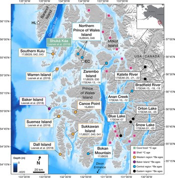
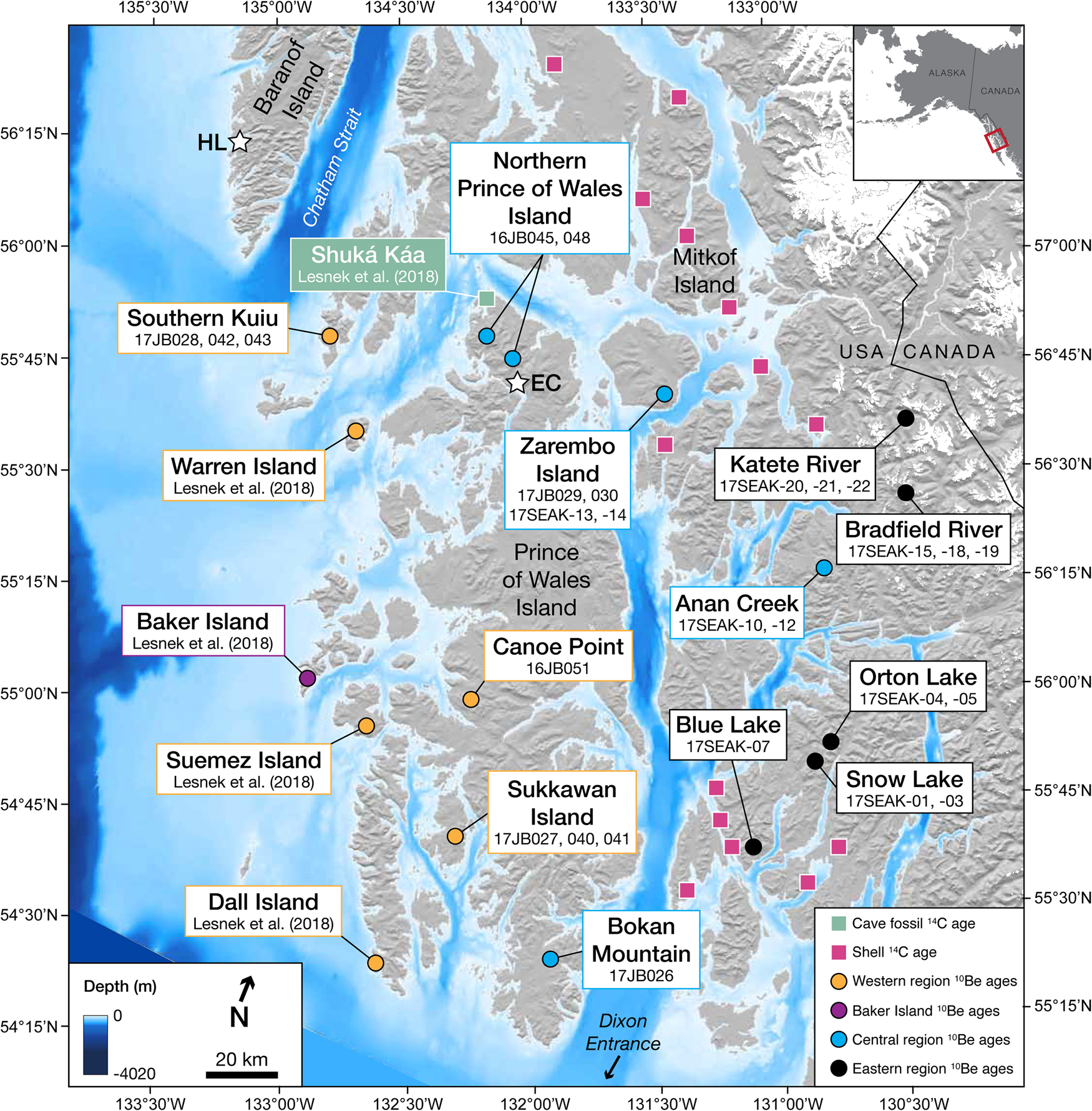
Map of study area. 10Be sampling sites are indicated by the dots. Sites are color coded, where yellow = western region, purple = Baker Island (local glaciers), blue = central region, and black = eastern region. 14C sampling locations are indicated by squares. Green = Shuká Káa cave (Lesnek et al., Reference Lesnek, Briner, Lindqvist, Baichtal and Heaton2018), pink = shell-bearing raised marine sediments. White stars indicate locations of previous work mentioned in the text. HL = Hummingbird Lake (Ager et al., Reference Ager2019), EC = El Capitan Cave (Wilcox et al., Reference Wilcox, Dorale, Baichtal, Spötl, Fowell, Edwards and Kovarik2019). Modern glacier extents (white) are from version 6 of the Randolph Glacier Inventory (NSIDC, 2005, updated 2018). (For interpretation of the references to color in this figure legend, the reader is referred to the web version of this article.)
METHODS
10Be dating
Sampling procedures and locations
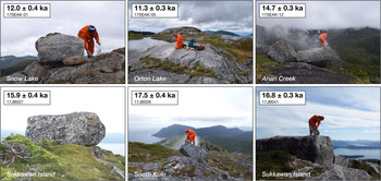
To directly date the timing of CIS recession, we sampled perched boulder (n = 24) and bedrock (n = 3) surfaces from 12 different locations in Southeast Alaska for 10Be exposure dating (Figs. 2 and 3). We sampled locations from the western coastline to the inland mountains with the goal of constraining deglaciation through the archipelago. Due to thick forest cover in low-lying regions, we targeted upland areas with exposed bedrock for sampling. Our sampling focused on granitic intrusions (Wilson et al., Reference Wilson, Hults, Mull and Karl2015), which allowed us to obtain sufficient quartz for 10Be dating. We collected samples from the upper ~2 cm of rock surfaces using a rock saw, hammer, and chisel. We recorded sample locations and elevations using a handheld GPS with ~5 m vertical uncertainty, and we measured topographic shielding using a clinometer. In general, sampling sites were located on the unvegetated tops of bedrock ridges or the outlets of small cirques; the sites ranged in elevation from 581 to 1345 m above sea level (m asl) (Table 1), well above the local marine limit (Shugar et al., Reference Shugar, Walker, Lian, Eamer, Neudorf, McLaren and Fedje2014; Carlson and Baichtal, Reference Carlson and Baichtal2015).
(color online) Examples of surfaces sampled for 10Be dating. 10Be ages are shown at 1 SD internal uncertainty. See online supplemental information for photographs of all samples.

10Be age information.
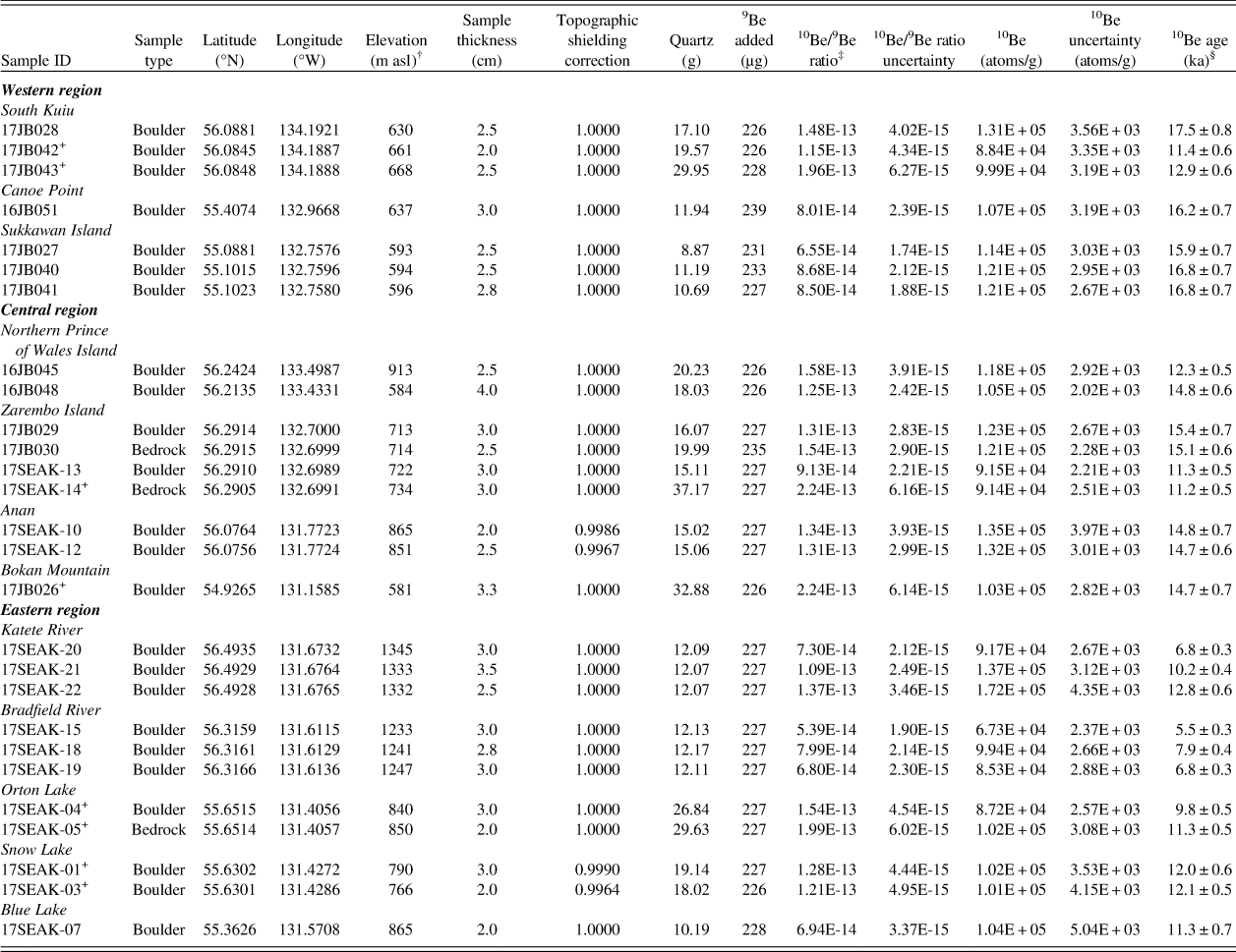
† Elevations and positions were recorded in the field with a Garmin handheld GPS receiver (~5 m vertical uncertainty).
‡ AMS results are standardized to 07KNSTD (Nishiizumi et al., Reference Nishiizumi, Imamura, Caffee, Southon, Finkel and McAninch2007); ratios are blank-corrected and shown at 1 SD uncertainty.
§ Be ages reported at 1σ external uncertainties and calculated with version 3 of the CRONUS-Earth calculator (Balco et al., Reference Balco, Stone, Lifton and Dunai2008) using the Arctic/Baffin Bay prouction rate (Young et al., Reference Young, Schaefer, Briner and Goehring2013) and Lm scaling.
'+ Measured at PRIME Lab; all other samples measured at Lawrence Livermore National Laboratory.
Here, we provide a more detailed description of each of the sampling sites. The first site, Southern Kuiu Island, lies just east of Chatham Strait, a deep glacially-scoured trough (Fig. 2). Samples from this site were collected from a ridge at ~650 m asl that separates several cirques. The second site, Canoe Point, is a small ridge that sits at ~640 m asl on central Prince of Wales Island. Our third site, Sukkawan Island, is ~3 km off the coast of Prince of Wales Island. We collected samples at this site from a ridge on the central portion of the island that lies ~590 m asl. At the fourth site on northern Prince of Wales Island, we collected two boulder samples on two unnamed rounded summits. These peaks are roughly 11 km south of Shuká Káa (125 m asl), an archeological site where mammal and bird bones ranging in age from more than 57 ka to modern have been excavated (Heaton and Grady, Reference Heaton, Grady, Schubert, Mead and Graham2003; Lesnek et al., Reference Lesnek, Briner, Lindqvist, Baichtal and Heaton2018). At the northern of the two summits, the boulder we sampled was perched on lichen-free bedrock at 913 m asl. At the southern peak, the sample was perched on lichen- and moss-covered bedrock.
The fifth site, Zarembo Island, sits ~40 km east of northern Prince of Wales Island. On Zarembo Island, we sampled rock surfaces on local topographic highs. Where exposed, the bedrock on this island was somewhat lichen-covered, and the few perched boulders that we found were low lying (~0.5 m in height). The sixth site, Anan Creek (~860 m asl), is a sculpted bedrock ridge that protrudes ~100 m above the valley floor; the exposure ages from this site record regional CIS deglaciation rather than retreat of local glaciers. Perched boulders at Anan Creek were plentiful and larger than those at other locations. Our seventh site, Bokan Mountain (~580 m asl), is situated on the southern tip of Prince of Wales Island. The site consisted of lichen-covered, sculpted bedrock.
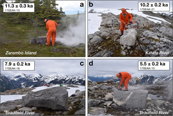
The eighth site, Katete River (~1330 m asl), is the highest elevation site in the study region. Exposed bedrock at this site had minimal lichen cover. We sampled three boulders from a local topographic high that protruded ~3 m above a snowfield that was present during sampling in July 2017 (Fig. 4). Two boulders were perched on bedrock, and one boulder was perched on a field of small, potentially frost-shattered cobbles. The ninth site, Bradfield River (~1240 m asl), also supported a snowfield during our sampling campaign in July 2017. The three boulders sampled at this site were perched on sculpted bedrock that jutted at least 4 m above the snowfield surface (Fig. 4). The tenth site, Orton Lake, is a bedrock ridge (~845 m asl) surrounded by steep drops (>500 m) on all sides. The bedrock at Orton Lake was ice-sculpted and had indicators of glacial erosion such as chattermarks. However, we found few large, stable perched boulders at this site; we sampled one of these boulders for 10Be dating. The eleventh site, Snow Lake, lies ~3 km southwest of Orton Lake. Snow Lake is a small cirque <1 km in diameter. We sampled two perched boulders near the cirque outlet. At the twelfth site, Blue Lake, we sampled one boulder on the right-lateral margin of a cirque. The cirque at Blue Lake was relatively small, and the boulder was located ~400 m from the headwall.
(color online) Samples with 10Be ages that are potentially impacted by snow shielding. Photos were taken during field work in July 2017. All 10Be ages are shown at 1 SD internal uncertainty. (A) Boulder from Zarembo Island. The boulder surface is lichen-covered, but the boulder is less than 1 m in height. (B) Boulder from the Katete River site. Note the largely lichen-free surface and snow field in the background. Sample is ~3 m above the snow surface. (C–D) Boulders from the Bradfield River site. The boulders are large and appear to be stable, but the lack of lichen on their surfaces may be indicative of seasonal snow cover. Samples are ~4 m above the snowfield surface.

Quartz isolation and accelerator mass spectrometry
Samples underwent physical and chemical preparation at the University at Buffalo Cosmogenic Isotope Laboratory using standard procedures (Kohl and Nishiizumi, Reference Kohl and Nishiizumi1992; Corbett et al., Reference Corbett, Bierman and Rood2016). Samples were processed in five separate batches and spiked with ~226-239 μg of 9Be (Table 1) using either the PRIME Lab low-level beryllium carrier (2017.11.17-Be; 9Be concentration of 1074 ± 8 ppm) or the GFZ German Research Centre for Geosciences Phenakite standard (9Be concentration of 372.5 ± 3.5 ppm). Accelerator mass spectrometry (AMS) was completed at Lawrence Livermore National Laboratory's Center for Accelerator Mass Spectrometry or PRIME Lab at Purdue University (Table 1). Samples measured at PRIME Lab were spiked with the PRIME Lab carrier, whereas samples measured at Lawrence Livermore National Lab were spiked with the GFZ Phenakite carrier. All sample ratios were measured with respect to the 07KNSTD standard, which has an assumed 10Be/9Be ratio of 2.85 × 10⁻¹² (Nishiizumi et al., Reference Nishiizumi, Imamura, Caffee, Southon, Finkel and McAninch2007). Sample ratios were corrected using batch-specific blank values that ranged from 1.17 × 10⁻¹⁵ to 3.35 × 10⁻¹⁵ (average = 2.25 × 10⁻¹⁵; n = 5). AMS analytical uncertainty ranged from 1.9 to 4.8%, with an average value of 2.8%.
10Be age calculations and assumptions
All ages were calculated using version 3 of the online CRONUS Earth exposure age calculator (hess.ess.washington.edu; Balco et al., Reference Balco, Stone, Lifton and Dunai2008; Balco, Reference Balco2017) using the Baffin Bay/Arctic production rate (Young et al., Reference Young, Schaefer, Briner and Goehring2013) and time-dependent (Lm) scaling (Lal, Reference Lal1991). For ease of comparison with the 14C ages from raised marine sediments, we subtracted 67 years from the raw 10Be ages; thus, all 10Be ages are reported with respect to AD 1950.
Changes in crust elevation over a rock surface's exposure duration result in a time-varying rate of 10Be production. Sample elevations can be corrected for this effect using regional emergence curves, which are constrained by either glacial isostatic adjustment models or relative sea level histories (Jones et al., Reference Jones, Whitehouse, Bentley, Small and Dalton2019). However, along the westernmost coast of Southeast Alaska, relative sea level history in the early deglacial period is largely unconstrained (Shugar et al., Reference Shugar, Walker, Lian, Eamer, Neudorf, McLaren and Fedje2014). A wave-cut terrace at ~165 m below sea level may correlate with a late Pleistocene lowstand (Carlson, Reference Carlson2007), but this feature is undated. The migration of a crustal forebulge (Carlson and Baichtal, Reference Carlson and Baichtal2015) through the outer islands of Southeast Alaska likely caused a relative sea level rise until ~10.6 ka, reaching a maximum of 25 m asl, followed by sea level fall to the present (Baichtal and Carlson, Reference Baichtal and Carlson2010). Farther inland, land surfaces experienced net isostatic uplift (i.e., relative sea level fall) following deglaciation, with a maximum elevation change of 191 m since ~13.7 ka. In addition, atmospheric compression above a sample site that has moved up or down in elevation, and shifts in the air pressure field due to a site's proximity to the ice margin, may counteract the effects of isostatic rebound on 10Be production rates (Staiger et al., Reference Staiger, Gosse, Toracinta, Oglesby, Fastook and Johnson2007). Due to (1) the variable and unconstrained nature of relative sea level change in this region, (2) the potential effects of changing atmospheric pressure through time at our sampling sites, and because (3) the production rate calibration dataset used to calculate our ages was not corrected for isostatic adjustment (Young et al., Reference Young, Schaefer, Briner and Goehring2013), we report our 10Be ages without elevation corrections.
We made no corrections for post-depositional erosion. We observed pristine, glacially-scoured surfaces on bedrock adjacent to our perched boulder samples, suggesting minimal surface erosion since deglaciation. Extended intervals of thick snow cover over a rock surface can lead to erroneously young apparent exposure ages. Modern snowfall data (since the 1940s) from the Western Regional Climate Center (https://wrcc.dri.edu/summary/Climsmak.html) indicates that most of the low-lying regions in Southeast Alaska have an average wintertime snow depth of fewer than 10 to 20 centimeters. It is likely that our high elevation sampling sites experienced more snow cover than the weather stations referenced above (see Discussion). However, the lack of snowfall data for these regions leads us to report our exposure ages without snow shielding corrections. Therefore, the 10Be ages reported here should be viewed as minimum exposure ages.
When interpreting 10Be surface exposure ages, an important consideration is the erosional capacity of the overriding ice. Overriding by weakly or non-erosive (i.e., cold-based) ice allows accumulated isotopes from previous exposure periods to remain in a surface (Bierman et al., Reference Bierman, Marsella, Patterson, Davis and Caffee1999; Corbett et al., Reference Corbett, Bierman, Graly, Neumann and Rood2013). To test for isotopic inheritance in our study area, we measured 10Be concentrations in adjacent boulder and bedrock surfaces.
14C dating
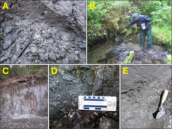
An extensive literature search and years of field reconnaissance have resulted in a dataset of over 620 shell-bearing raised marine deposits throughout Southeast Alaska. A select subset of this data is reported here. Samples of shell-bearing strata were found in various locations across the islands of Southeast Alaska. We collected material from raised marine deposits at 25 sites across the study area (Fig. 2) following the procedures outlined in Carlson and Baichtal (Reference Carlson and Baichtal2015). Many sites were exposed during road, quarry, or building excavations. Some are from deposits exposed in landslides, river and creek beds, or along wave-cut shorelines. In general, the deposits were stratified (Fig. 5), and where possible, samples were collected from multiple layers within the same set of sediments. Elevation measurements were taken using hand-held barometric digital altimeters accurate to ± 1 m and were zeroed twice daily. When possible, LiDAR-generated data points were averaged to obtain elevations or to create a local datum. All elevations were calculated relative to mean lower low water (MLLW), measured multiple times, and averaged. Subsequently, some elevations were verified from LiDAR data acquired in 2017 and 2018.
(color online) Representative raised marine sediments and samples for 14C dating. (A) Shells embedded in raised marine sediments on Mitkof Island. (B) Marine sediments on Wrangell Island. (C) Section of raised marine sediments from Kupreanof Island. (D) Shells from Gravina Island. (E) Section of raised marine sediments on Revillagigedo Island.

Bulk samples were taken of the shell materials and carried from the field in gallon-sized resealable plastic bags. Recovered samples were washed and screened though two graduated U.S.A. Standard Testing Sieves, #16, 1.18 microns (0.0469 inches) and #200, 0.075 microns (0.0029 inches). Samples were air-dried. Large shells, bone and wood samples were separated out for identification to genus and species when possible. The finer sediment was examined under varying magnification and handpicked for shell, fish bone, charcoal, wood and plant fragments, foraminifera, ostracods, and otoliths and identified to genus and species when possible. To ensure that that long-lived shell species would not bias the dating process, fragments of small shells, gastropods, and barnacle plates were selected for dating. Because living clams can burrow through sediment to a great depth, effectively burrowing into older strata, paired valves in growth position were not dated. However, samples of paired valves in growth position were collected for species identification. We also collected barnacles and serpulid worm casts for dating (Table 2). In all, these invertebrates are generally found in the intertidal to subtidal zones, and provide closely-limiting constraints on sea level, and therefore CIS retreat.
14C age information.

Samples were prepared for AMS measurements at the Beta Analytic laboratory or the USGS 14C Laboratory, and 14C measurements were completed at Beta Analytic or Lawrence Livermore National Laboratory. We corrected shell ages using a locally calibrated marine reservoir age, where ΔR is 700 years (total reservoir correction = 1100 years; Josenhans et al., Reference Josenhans, Fedje, Pienitz and Southon1997; Addison et al., Reference Addison, Beget, Ager and Finney2010). Ages were calculated in OxCal version 4.3 (Bronk Ramsey, Reference Bronk Ramsey2009) using the Marine13 calibration curve (Reimer et al., Reference Reimer, Bard, Bayliss, Beck, Blackwell, Ramsey, Buck, Cheng, Edwards and Friedrich2013), and are shown at two standard deviation (2 SD) uncertainty.
Ice flow mapping
To reconstruct CIS flow direction, we identified and mapped glacial flow indicators across coastal Southeast Alaska through a combination of field reconnaissance and remote sensing. Throughout the study area, we measured the direction of 231 striations in the field using a handheld compass. We also identified land-based ice flow indicators such as drumlins and crag and tail features using publicly available LiDAR Digital Terrain Models (DTMs) for Prince of Wales Island from the Alaska Division of Geological and Geophysical Surveys (https://elevation.alaska.gov). The LiDAR surveys were flown in 2017 and the resulting DTMs have a vertical accuracy of 19.6 cm or better at the 95% confidence interval. We created hillshade maps of Prince of Wales Island using an illumination azimuth and inclination of 315° and 30°, respectively. In addition, we mapped streamlined bedforms, such as drumlins and mega-scale glacial lineations, on the seafloor using Bathymetric Attributed Grid (BAG) shaded relief maps downloaded from the NOAA National Centers for Climate Information (https://maps.ngdc.noaa.gov/viewers/bathymetry/).
RESULTS
10Be ages
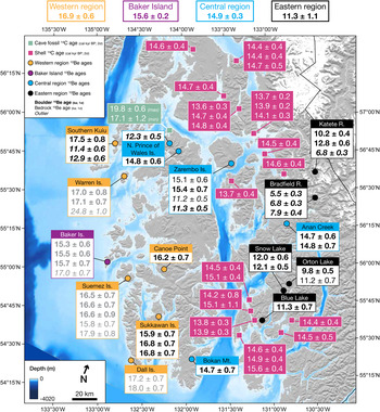
All 10Be ages are discussed in the following paragraphs are presented in Figure 6. Normalized kernel density estimates for each site are shown in Figures 7 through 9, and Figure 10 shows combined normalized kernel density estimates. All 10Be ages reported at 1 SD external uncertainty, which includes production rate uncertainty.
Map of Southeast Alaska with deglaciation chronology. Ages are color coded by type and region.14C ages from Shuká Káa (Lesnek et al., Reference Lesnek, Briner, Lindqvist, Baichtal and Heaton2018) are shown in green boxes with white text. Minimum-limiting 14C ages from raised marine sediments are shown in pink boxes with white text. All 14C ages are calibrated and shown at 2 SD uncertainty. 10Be ages from this study are shown in white boxes with black text. Previously published 10Be ages (Lesnek et al., Reference Lesnek, Briner, Lindqvist, Baichtal and Heaton2018) are indicated with gray text. Boulder ages are in bold text, bedrock ages are in normal text. All 10Be ages are color coded by region: yellow = western region, purple = Baker Island (local glaciers), blue = central region, and black = eastern region. Outliers are indicated by italic text. All 10Be ages are shown at 1 SD external uncertainty. Average 10Be ages for each region (mean ± 1 SD) are shown at the top of the image. (For interpretation of the references to color in this figure legend, the reader is referred to the web version of this article.)

(color online) Normalized kernel density estimates for 10Be ages in the western region of the study area. All 10Be ages are plotted with 1 SD internal uncertainty. In the bottom panel, all ages from the western region are summed, and the average age for the western region group excludes three outliers (two young outliers, one old outlier that is not pictured) that were 2 SD outside of the mean.

On southern Kuiu Island, exposure ages from three perched boulders are 17.5 ± 0.8, 12.9 ± 0.6, and 11.4 ± 0.6 ka. At Canoe Point on west central Prince of Wales Island, a perched boulder yields an exposure age of 16.2 ± 0.7 ka. On Sukkawan Island, west of Prince of Wales Island, three perched boulders have exposure ages of 15.9 ± 0.7, 16.8 ± 0.7, and 16.8 ± 0.7 ka. Combined with nine 10Be ages previously reported by Lesnek et al. (Reference Lesnek, Briner, Lindqvist, Baichtal and Heaton2018), the average exposure age for this outer region is 16.9 ± 0.6 ka (mean ± 1 SD; n = 12; Fig. 7). This average excludes three outliers, which fall more than 2 SD outside of the mean (15SEAK-12, 17JB042, 17JB043; Table 1).
On northern Prince of Wales Island, two boulders have exposure ages of 14.8 ± 0.5 and 12.3 ± 0.5 ka. On Zarembo Island, two perched boulders yield exposure ages of 15.4 ± 0.7 and 11.3 ± 0.5 ka, and two bedrock surfaces have exposure ages of 15.1 ± 0.6 and 11.3 ± 0.2 ka. At Anan Creek, two boulders yield 10Be ages of 14.7 ± 0.6 and 14.8 ± 0.7 ka. Finally, at Bokan Mountain on southern Prince of Wales Island, one perched boulder has an exposure age of 14.7 ± 0.7 ka. Although these four sites are separated by as much as 150 km in the north-south direction, we find no trend in age across the region; we therefore average all the 10Be ages for the central region. Excluding three young outliers whose ages fall more than 2 SD outside the mean of the population (16JB045, 17SEAK-13, 17SEAK-14; Table 1), the 10Be ages average 14.9 ± 0.3 ka (mean ± 1 SD; n = 6; Fig. 8).
(color online) Normalized kernel density estimates for 10Be ages in the central region of the study area. All 10Be ages are plotted with 1 SD internal uncertainty. In the bottom panel, all ages from the central region are summed, and the average age for the central region excludes three young outliers.

Normalized kernel density estimates for 10Be ages in the eastern region of the study area. In the bottom panel, all ages from the eastern region are summed, and the average age for the eastern region excludes six young outliers.

(color online) Normalized kernel density estimates for 10Be ages in all regions in the study area, including Baker Island.

At the Katete River site (~1335 m asl), three boulder ages have exposure ages of 12.8 ± 0.6, 10.2 ± 0.4, and 6.8 ± 0.3 ka. At the Bradfield River site (~1240 m asl), three boulders perched directly on bedrock or smaller clasts on bedrock yield 10Be ages of 7.9 ± 0.4, 6.8 ± 0.3, and 5.5 ± 0.3 ka. At Orton Lake, we sampled a perched boulder and the upper surface of a sculpted bedrock ridge. The boulder has a 10Be age of 9.8 ± 0.5 ka, whereas the sculpted bedrock has a 10Be age of 11.3 ± 0.5 ka. At Snow Lake, two boulders in a small cirque yield ages of 12.1 ± 0.5 and 12.0 ± 0.6 ka. At Blue Lake, one perched boulder on the right-lateral margin of a small cirque has an exposure age of 11.3 ± 0.7 ka.
14C ages
The dated materials from raised marine deposits across the field area (Figs. 5 and 6) provide minimum-limiting constraints on CIS deglaciation. The elevations of these deposits are not consistent across the study area; this variability is due to differential isostatic uplift since deglaciation. The ages range from 13,610 ± 300 to 15,580 ± 370 cal yr BP (n = 25), and there is no spatially coherent pattern with age.
CIS extent and flow direction
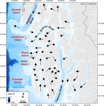
Based on our 10Be dating in the western region (this study; Lesnek et al., Reference Lesnek, Briner, Lindqvist, Baichtal and Heaton2018) and seafloor geomorphology (see Methods), we reconstructed the maximum extent of the CIS during the latest Pleistocene (Fig. 11). Previously published chronology indicates that CIS maximum extent was achieved between ~20 and 17 ka (Lesnek et al., Reference Lesnek, Briner, Lindqvist, Baichtal and Heaton2018). This updated mapping builds on work published by Carrara et al. (Reference Carrara, Ager and Baichtal2007), who identified several areas along the western coast of Southeast Alaska that may have served as ice-free refugia during the LGM. In our refined reconstruction (Fig. 11), Dall, Suemez, and Warren Islands, which were listed as potential refugia by Carrara et al. (Reference Carrara, Ager and Baichtal2007), are covered by ice during the CIS maximum stage because 10Be ages from these islands indicate deglaciation at ~17 ka (this study; Lesnek et al., Reference Lesnek, Briner, Lindqvist, Baichtal and Heaton2018). However, because we do not have exposure ages from other locations identified as potential refugia by Carrara et al. (Reference Carrara, Ager and Baichtal2007), including portions of Baranof, Coronation, Noyes, Baker, and Forrester islands, we cannot rule out the possibility that those locations escaped cover by the CIS (but perhaps not local glaciers) during the regional LGM (Fig. 11). As such, in this updated reconstruction, we follow the original interpretations of Carrara et al. (Reference Carrara, Ager and Baichtal2007) and leave these areas ice-free. While the ice extent map presented here is an improvement on previous work, we emphasize that this new map is largely speculative, and needs to be further refined with chronology from the potential refugia.
Map of inferred CIS maximum extent (~20-17 ka) and flow direction during the latest Pleistocene. CIS extent (white lines and shading) is updated from Carrara et al. (Reference Carrara, Ager and Baichtal2007) and inferred from 10Be ages in the western region of the study area and bathymetry. Ice-free refugia may have existed on Baranof, Coronation, Noyes, Baker, and Forrester islands (red text). Black arrows represent average ice flow based on groups of at least five directional indicators, such as striations, drumlins, and crag and tails. For additional details on the ice flow indicators, we direct the reader to the online supplementary information. (For interpretation of the references to color in this figure legend, the reader is referred to the web version of this article.)

LiDAR-based Digital Evaluation Models (DEMs) of Prince of Wales Island reveal hundreds of ice flow indicators, including crag and tail features (n = 336) and drumlins (n = 1249). These features vary in both size and density on the landscape, with the largest and most concentrated occurrences appearing on the eastern side of Prince of Wales Island, flowing into Clarence Strait (see online supplemental material). We also used striations preserved on bedrock to infer flow direction throughout the study region (Fig. 11). In some cases, striations close to one another are not parallel, suggesting either complex local flow during the last glacial period or multiple phases of ice flow during deglaciation. Additionally, streamlined bedforms up to 5 km in length are found on the seafloor in Clarence, Sumner, and Chatham straits (Fig. 11). These bedforms generally follow topography, and may be indicative of grounded ice streams during the LGM (Eyles et al., Reference Eyles, Moreno and Sookhan2018).
DISCUSSION
Chronology of Cordilleran Ice Sheet retreat in Southeast Alaska
Based on the clustering of 10Be ages across the study area (Fig. 10), we have grouped the sites into three distinct phases of glacial retreat. The first group, which we term the “western region,” encompasses sites that date the initial retreat of the CIS from what is now the westernmost coast of Southeast Alaska. The second group, termed the “central region,” is composed of sites that track CIS recession through the fjords in Southeast Alaska. The last group, the “eastern region,” consists of cirque floors or ridgetops between cirques that date the final retreat of small glaciers independent of the CIS.
Our 10Be ages from perched boulders and bedrock in the western region place ice retreat from the outer islands of the Alexander Archipelago at 16.9 ± 0.6 ka (mean ± 1 SD; n = 12). The anomalously old exposure age from bedrock on Warren Island (15SEAK-12; 24.8 ± 1.0 ka) is likely due to inherited 10Be that accumulated prior to the most recent deglaciation and was previously discussed in Lesnek et al. (Reference Lesnek, Briner, Lindqvist, Baichtal and Heaton2018). We identified two young outliers at the Southern Kuiu Island site: one perched boulder (17JB042; 11.4 ± 0.6 ka; boulder height ~1.25 m) and one bedrock sample (17JB043; 12.9 ± 0.6 ka). The coastal location of the site, the lichen-covered boulder surface, and the sample elevation (~665 m asl) suggest that in modern times, the site does not experience much snow accumulation during the winter months. A 1.5-m-tall perched boulder ~400 m north of the above samples returned an exposure age of 17.5 ± 0.8 ka, which aligns well with 10Be ages from other perched boulders and bedrock in our western region (Lesnek et al., Reference Lesnek, Briner, Lindqvist, Baichtal and Heaton2018).
The 10Be ages from the central region of the study area suggest the CIS evacuated the fjords in coastal Southeast Alaska by 14.9 ± 0.3 ka (mean ± 1 SD; n = 6). This average excludes three ages from two locations in the central region: northern Prince of Wales Island and Zarembo Island. The age of 12.3 ± 0.5 ka from a boulder on northern Prince of Wales Island (Fig. 6; 16JB045) may be too young due to sediment shielding, or perhaps snow shielding as the sample lies at a relatively high elevation of 913 m asl. The 10Be ages from Zarembo Island are more difficult to interpret. We collected two boulder-bedrock pairs at this site, and one pair returned ages of ~15.3 ka while the other pair yielded exposure ages of ~11.3 ka (Fig. 6). The boulder-bedrock pairs come from similar locations, and are separated by fewer than 100 m laterally. The younger ages are from a slightly higher elevation (~730 vs. ~713 m asl). The two boulders collected from this site are also similar in height and their degree of lichen cover, and both boulders were perched on vegetated (currently stable) bedrock. From this site alone, it would be challenging to determine which of the two boulder-bedrock pairs more accurately dates the timing of CIS retreat. However, 10Be ages from elsewhere in the central region and the minimum-limiting 14C ages from raised marine sediments (Fig. 6) suggest the CIS had evacuated southern Southeast Alaska's fjords sometime between ~15.6 and 13.6 cal ka BP. This interpretation is supported by previous work in the region; for example, radiocarbon-dated marine sediments suggest the outlet glacier occupying Dixon Entrance (Fig. 2) had receded to the modern coastline by ~14.5 cal ka BP (Barrie and Conway, Reference Barrie and Conway1999). Additionally, on southwestern Baranof Island (Fig. 2), 14C-dated lake sediments suggest ice-free conditions by ~14.6 cal ka BP (Ager, Reference Ager2019). In all, the available chronology suggests that the ~15.3 ka ages on Zarembo Island are more likely accurately dating regional deglaciation than the ~11.3 ka ages. Thus, the older ages from Zarembo Island are included in the regional average 10Be age of 14.9 ± 0.3 ka (mean ± 1 SD; n = 6).
The 10Be ages from inland cirques and ridges are more scattered than those from the other two regions (Figs. 6 and 9), and consequently definitive interpretations are more difficult to make. Scatter in the exposure ages is particularly apparent at the Bradfield River and Katete River sites, which are both situated >1200 m asl. These sites host snowfields that persisted through the summer in 2017 (Fig. 4). Boulders at these sites lacked significant lichen cover on their surfaces, suggesting that even under modern climatic conditions, they retain persistent snow cover throughout most of the year. Thus, the 10Be ages from the Bradfield and Katete river sites should strictly be viewed as minima. Ages from the southern sites in the eastern region (Orton, Snow, and Blue lakes) are more coherent; samples are from lower elevations and field evidence is less consistent with persistent snow cover. Samples from Orton, Snow, and Blue lakes return exposure ages that average 11.3 ± 1.1 ka (mean ± 1 SD; n = 5). This age for deglaciation at these sites is supported by 36Cl exposure ages from glacially-abraded bedrock on the summit of Mitkof Island (Fig. 2), which indicate deglaciation by ~11.3 ka (Viens, Reference Viens2001). In aggregate, our results from the eastern region suggest that local glaciers were probably present in the southern Southeast Alaskan Coast Mountains until at least the early Holocene.
In all three regions of the study area, we find surfaces with early Holocene exposure ages (Fig. 10). At one site in the western region (Southern Kuiu Island) and two sites in the central region (northern Prince of Wales Island and Zarembo Island), these surfaces are several thousand years younger than the mean deglaciation age, which is 16.9 ± 0.6 ka and 14.9 ± 0.3 ka, respectively. When combined with 10Be ages from the eastern region, these samples average 11.5 ± 0.9 ka (n = 12). The clustering of ages about this mean, at sites that are separated in some cases by more than 150 km, suggests these ages may have climatic significance, which we discuss further below.
Cordilleran Ice Sheet deglaciation across the North Pacific
Our results are consistent with previously published reconstructions from other marine-terminating CIS margins along the North Pacific coast, implying that broad regions of the ice sheet behaved synchronously during deglaciation. Our ages from the western region suggest that initial CIS retreat was underway by ~17 ka. Immediately to the south of our study area, 14C ages from Haida Gwaii and nearby Hecate Strait (Fig. 1) suggest the CIS may have been retreating as early as ~19 ka (Clague et al., Reference Clague, Mathewes and Warner1982; Blaise et al., Reference Blaise, Clague and Mathewes1990; Mathewes and Clague, Reference Mathewes and Clague2017). Farther south, 10Be ages from Calvert Island (Fig. 1) suggest that the CIS had retreated to the modern coastline at ~18 ka (Darvill et al., Reference Darvill, Menounos, Goehring, Lian and Caffee2018). Similarly, terrestrial 14C ages from Kodiak Island, southern Alaska (Mann and Peteet, Reference Mann and Peteet1994), and the Alaska Peninsula Glacier Complex (Misarti et al., Reference Misarti, Finney, Jordan, Maschner, Addison, Shapley, Krumhardt and Beget2012) indicate initial glacier retreat ~17 ka (Fig. 1). Ice-rafted debris records from the Southeast Alaska margin (Praetorius et al., Reference Praetorius, Mix, Jensen, Froese, Milne, Wolhowe, Addison and Prahl2016), the Vancouver Island shelf (Fig. 12g; Cosma et al., Reference Cosma, Hendy and Chang2008), and the coastal Gulf of Alaska (Praetorius and Mix, Reference Praetorius and Mix2014) show a period of intense iceberg calving around North Pacific beginning between ~18 and 17 ka. Likewise, observations of surface freshening in the central Gulf of Alaska (Fig. 12c; Davies et al., Reference Davies, Mix, Stoner, Addison, Jaeger, Finney and Wiest2011; Maier et al., Reference Maier, Zhang, Abelmann, Gersonde, Mulitza, Werner, Méheust, Ren, Chapligin and Meyer2018) suggest widespread calving of the western CIS beginning ~18 ka.
Glacial and climate history of the Pacific coast. (A) GISP2 δ18O (Grootes and Stuiver, Reference Grootes and Stuiver1997). (B) Global eustatic sea level stack (Spratt and Lisiecki, Reference Spratt and Lisiecki2016). (C) Gulf of Alaska surface δ18O from marine sediment core SO202-27-6, which relates to salinity (Maier et al., Reference Maier, Zhang, Abelmann, Gersonde, Mulitza, Werner, Méheust, Ren, Chapligin and Meyer2018). (D) Sea surface temperatures derived from alkenones in marine sediment core EW0408-85JC (Praetorius et al., Reference Praetorius, Mix, Walczak, Wolhowe, Addison and Prahl2015). (E) Surface (light blue dotted line) and subsurface (dark blue solid line) ocean temperatures derived from Mg/Ca ratios in foraminifera in marine sediment core MD02-2946 (Taylor et al., Reference Taylor, Hendy and Pak2014). (F) Time distance diagrams for the marine-terminating CIS margin in coastal Southeast Alaska. Circles represent average 10Be ages plotted against distance from the CIS maximum extent, color coded by group. Triangles are 14C ages; green triangles are 14C ages on ringed seal bones in Shuká Káa (Lesnek et al., Reference Lesnek, Briner, Lindqvist, Baichtal and Heaton2018), pink triangles are on shells in raised marine sediments (this study). (G) Ice-rafted debris in marine sediment core MD02-2946, offshore Vancouver Island (Cosma and Hendy, Reference Cosma and Hendy2008). (For interpretation of the references to color in this figure legend, the reader is referred to the web version of this article.)

Radiocarbon-dated marine sediments suggest that following the onset of deglaciation, marine-terminating CIS margins receded through fjords across Southeast Alaska and British Columbia until about ~15 ka (Mann and Hamilton, Reference Mann and Hamilton1995; Barrie and Conway, Reference Barrie and Conway1999; Lacourse and Mathewes, Reference Lacourse, Mathewes, Fedje and Mathewes2005). In the central Gulf of Alaska, sea surface salinity and ice-rafted debris deposition decreased between ~16 and 15 ka (Fig. 12c; Maier et al., Reference Maier, Zhang, Abelmann, Gersonde, Mulitza, Werner, Méheust, Ren, Chapligin and Meyer2018), indicating that some formerly marine-terminating CIS termini began to recede onto land at this time, which reduced the delivery of icebergs and ice sheet meltwater to the open ocean. Radiocarbon-dated glaciomarine sediments from core EW0408-85JC on the southern Alaskan margin (Fig. 1) suggest major CIS outlet glaciers had transitioned from marine-terminating to land-terminating by ~14.8 ka (Davies et al., Reference Davies, Mix, Stoner, Addison, Jaeger, Finney and Wiest2011). This period coincides with an interval of marked CIS thinning in coastal British Columbia (Darvill et al., Reference Darvill, Menounos, Goehring, Lian and Caffee2018), and evidence from Baker Island demonstrates that local glaciers in coastal Southeast Alaska also disappeared by ~15.5 ka (Fig. 6; Lesnek et al., Reference Lesnek, Briner, Lindqvist, Baichtal and Heaton2018). Taken together, the available data point to widespread retreat of marine-terminating CIS margins between ~18 and 15 ka.
Retreat of western CIS margins continued after ~15 ka, and by the early Holocene what remained of the CIS was restricted to mainland British Columbia (Margold et al., Reference Margold, Jansson, Kleman, Stroeven and Clague2013; Margold et al., Reference Margold, Stroeven, Clague and Heyman2014; Menounos et al., Reference Menounos, Goehring, Osborn, Margold, Ward, Bond, Clarke, Clague, Lakeman and Koch2017). In the absence of major CIS outlet glaciers, high-elevation areas fringing the Pacific coast likely hosted small, localized ice caps and cirque glaciers (Fedje and Mathewes, Reference Fedje and Mathewes2005), but the history of glacier change along the Pacific coast between ~15 ka and the onset of the Holocene at 11.7 ka is unknown. Glacier readvances in the interior regions of British Columbia occurred during the Younger Dryas (Menounos et al., Reference Menounos, Goehring, Osborn, Margold, Ward, Bond, Clarke, Clague, Lakeman and Koch2017), but from the data presented here, it is unclear if similar readvances occurred in Southeast Alaska. Additional detailed, site-specific work should take place to further constrain Younger Dryas and Holocene glacier fluctuations in Southeast Alaska. By 11 ka, ice in western Canada had retreated significantly from its late Pleistocene maximum (Clague, Reference Clague2017), consistent with our results from the Southeast Alaskan coast.
Causes of marine-terminating Cordilleran Ice Sheet change
The shift from the end of the LGM (~19 ka) to the start of the Holocene interglacial was accompanied by dramatic changes in global eustatic sea level (Spratt and Lisiecki, Reference Spratt and Lisiecki2016), ocean temperature (Bereiter et al., Reference Bereiter, Shackleton, Baggenstos, Kawamura and Severinghaus2018), and air temperature (Shakun et al., Reference Shakun, Clark, He, Marcott, Mix, Liu, Otto-Bliesner, Schmittner and Bard2012). In addition, the glaciological structure of the CIS may have shifted when the ice sheet reached its maximum volume, resulting in the formation of large ice streams in many regions along the Pacific coast (Eyles et al., Reference Eyles, Moreno and Sookhan2018). In this section, we explore the potential impact of each of these factors on CIS change in Southeast Alaska and western British Columbia during the last deglaciation.
Based on our record in coastal Southeast Alaska as well as other records across the North Pacific (Blaise et al., Reference Blaise, Clague and Mathewes1990; Cosma and Hendy, Reference Cosma and Hendy2008; Praetorius and Mix, Reference Praetorius and Mix2014; Praetorius et al., Reference Praetorius, Mix, Jensen, Froese, Milne, Wolhowe, Addison and Prahl2016; Maier et al., Reference Maier, Zhang, Abelmann, Gersonde, Mulitza, Werner, Méheust, Ren, Chapligin and Meyer2018), the period between ~18 and 15 ka was one of intense calving of marine-terminating CIS margins. One mechanism that may have triggered widespread ice sheet retreat was sea level rise in the early deglacial period. Somewhat unusually for recently deglaciated landscapes (which typically experience relative sea level fall due to isostatic rebound), sea level in Southeast Alaska and western British Columbia likely rose during the early deglacial period due to a combination of eustatic sea level rise (Fig. 12b; Spratt and Lisiecki, Reference Spratt and Lisiecki2016) and the migration and collapse of a crustal forebulge (Addison et al., Reference Addison, Beget, Ager and Finney2010; Shugar et al., Reference Shugar, Walker, Lian, Eamer, Neudorf, McLaren and Fedje2014; Carlson and Baichtal, Reference Carlson and Baichtal2015). These two processes, when working together, could have destabilized grounded ice margins and driven iceberg production (Clague, Reference Clague and Fulton1989) during the early deglacial period. The presence of streamlined bedforms in troughs around the Pacific coast suggests that CIS outlet glaciers (and possibly ice streams; see Eyles et al., Reference Eyles, Moreno and Sookhan2018) in Southeast Alaska and British Columbia were grounded in their fjords when the CIS was at its maximum extent (Herzer and Bornhold, Reference Herzer and Bornhold1982; Blaise et al., Reference Blaise, Clague and Mathewes1990). These fast-flowing ice margins may have been especially vulnerable to sea-level-driven instability (Hendy and Cosma, Reference Hendy and Cosma2008; Bassis et al., Reference Bassis, Petersen and Mac Cathles2017; Eyles et al., Reference Eyles, Moreno and Sookhan2018).
Warming of the ocean in contact with ice sheet margins may have contributed to initial CIS retreat at ~17 ka (Joughin et al., Reference Joughin, Alley and Holland2012), and several studies have documented major changes in eastern Pacific Ocean conditions during the last deglaciation. On the Vancouver Island shelf, Mg/Ca ratios in surface- and subsurface-dwelling foraminifera show warming of ~2°C and ~5°C, respectively, between ~17.2 and 15 ka (Fig. 12e; Taylor et al., Reference Taylor, Hendy and Pak2014). A similar warming trend was underway by ~18 ka on the Gulf of Alaska shelf, with peak temperatures reached by ~14 ka following a warming of ~9°C. (Fig. 12d; Praetorius et al., Reference Praetorius, Mix, Walczak, Wolhowe, Addison and Prahl2015). However, between ~14 and 12 ka (i.e., during the Bølling-Allerød and Younger Dryas), surface temperatures in the Gulf of Alaska decreased by ~5°C (Praetorius et al., Reference Praetorius, Mix, Walczak, Wolhowe, Addison and Prahl2015). Due to the lack of detailed glacial chronology in Southeast Alaska during this interval, the influence of these fluctuations in ocean temperature just before the Pleistocene-Holocene transition on CIS and local glacier mass balance is unknown.
Changes in atmospheric temperature and precipitation could have enhanced the CIS margin response to sea level rise and ocean warming. Yet, because the CIS covered much of the Pacific coast until ~15 ka, terrestrial paleoclimate archives that span the early deglacial period are scarce. One of the few available continuous deglacial climate records comes from the Mt. Logan ice core; however, Fisher et al. (Reference Fisher, Osterberg, Dyke, Dahl-Jensen, Demuth, Zdanowicz, Bourgeois, Koerner, Mayewski and Wake2008) suggest variations in ice core δ18O correlate to changes in source region rather than temperature, and the chronology in the earlier part of the record is somewhat imprecise. In Southeast Alaska, Ager (Reference Ager2019) generated a ~15 ka pollen record from Hummingbird Lake on southwestern Baranof Island (Fig. 2). The pollen record from this site documents several shifts in vegetation communities (and thus climate) during the Pleistocene–Holocene transition. From ~15 to 14 ka, pine (Pinus) species are the most abundant, which are interpreted to represent relatively warm temperatures. Similarly, on Haida Gwaii, which is thought to have hosted only local glaciers during the LGM (Clague, Reference Clague and Fulton1989), terrestrial vegetation became established by ~15 ka (Lacourse and Mathewes, Reference Lacourse, Mathewes, Fedje and Mathewes2005), suggesting the first significant post-glacial warming did not occur until then (Mathewes and Clague, Reference Mathewes and Clague2017). In Hummingbird Lake, increases in alder (Alnus) pollen percentage and decreases in pine pollen percentage between ~14 and 11 ka suggest that air temperatures generally cooled, a result that is consistent with marine temperature reconstructions across the North Pacific (Taylor et al., Reference Taylor, Hendy and Pak2014; Praetorius et al., Reference Praetorius, Mix, Walczak, Wolhowe, Addison and Prahl2015). If this cooling occurred during the summer months, it may have slowed CIS retreat, or perhaps even triggered readvances of the CIS and/or local glaciers before the onset of the Holocene (e.g., Menounos et al., Reference Menounos, Goehring, Osborn, Margold, Ward, Bond, Clarke, Clague, Lakeman and Koch2017).
Our results indicate that local glaciers (in the eastern region) and persistent snow patches (in the western and central regions) lingered in coastal Southeast Alaska until the early Holocene. What caused the demise of these glaciers and snow patches? At present, terrestrial climate conditions in the region have been reconstructed from pollen assemblages and speleothem records. The appearance of Sitka spruce (Picea sitchensis), mountain hemlock (Tsuga mertensiana), and western hemlock (Tsuga heterophylla) pollen in Hummingbird Lake sediments after ~11 ka is interpreted as a response to warming summer air temperatures at the beginning of the Holocene (Ager, Reference Ager2019). These interpretations from pollen are corroborated by cave deposits from El Capitan Cave on northern Prince of Wales Island (Fig. 2; Wilcox et al., Reference Wilcox, Dorale, Baichtal, Spötl, Fowell, Edwards and Kovarik2019). There, a hiatus in speleothem deposition between and 41.5 ± 0.2 and 13.4 ± 0.2 ka BP suggests the presence of discontinuous permafrost and/or the CIS, and therefore mean annual air temperatures below 0°C, during MIS 2 and the early deglacial period. Stable oxygen isotope measurements on speleothem material that dates from 13.4 ± 0.2 to 11.1 ± 0.3 ka BP show warming temperatures in the late Bølling-Allerød followed by mild cooling during the Younger Dryas, then a return to warmer conditions at the start of the Holocene (Wilcox et al., Reference Wilcox, Dorale, Baichtal, Spötl, Fowell, Edwards and Kovarik2019). This interval of summertime warming in Southeast Alaska after ~11 ka, identified in two independent archives, may have been sufficient to drive retreat of local glaciers in the Coast Mountains and also melt persistent snow patches in the western and central regions of the study area, resulting in surfaces with early Holocene exposure ages in these three regions (Figs. 6 and 10).
To summarize, in Southeast Alaska and western British Columbia, the initial retreat of marine-terminating CIS margins from their maximum extent was probably driven by factors acting on the ice-ocean interface, including sea level rise and ocean warming, leading to intense ice loss via calving in the early stages of deglaciation. The sensitive response of marine-terminating CIS regions to sea level and ocean temperature change during the early deglacial period may have been a consequence of the onset of ice streaming once the CIS reached its maximum volume (Eyles et al., Reference Eyles, Moreno and Sookhan2018). During the later stages of deglaciation (after ~15 ka), terrestrial climate reconstructions suggest that atmospheric warming also contributed to CIS margin recession.
CONCLUSIONS
We present a new chronology for the recession of a marine-terminating CIS margin in southern Southeast Alaska. Our results suggest that ice retreat occurred in two pulses, with an initial phase occurring between ~17 and 15 ka, as ice retreated from the outermost coast through the major fjords. This retreat may have been a result of eustatic sea level rise and oceanic warming acting in concert to destabilize grounded outlet glaciers and/or ice streams. After ~15 ka, the CIS retreated into inland British Columbia, eventually leaving only small, localized ice caps in high-elevation areas that receded by ~11 ka. Due to a lack of chronology between ~15 and 11 ka, at this time our record cannot be used to assess the response of local glaciers in Southeast Alaska to hemispheric climate events such as the Younger Dryas. Overall, our reconstruction of deglaciation is consistent with other findings in marine-terminating CIS regions, suggesting a widespread response of the western CIS to deglacial climate change, including oceanic and perhaps atmospheric warming.
ACKNOWLEDGMENTS
The authors would like to thank Risa J. Carlson, Jane L. Smith, Dennis J. Landwehr, Katherine Prussian, Anna Harris, and Nicholas Schmuck for assistance in the field, and Christopher Sbarra for assistance in the field and the lab. Christopher Darvill and Nick Eyles provided thoughtful comments that improved this manuscript. Funding for this research was provided by an NSF Doctoral Dissertation Research Improvement Grant to Jason P. Briner and Alia J. Lesnek (award no. BCS-1657065) and by the Tongass National Forest Geology Program of the U.S. Forest Service.
SUPPLEMENTARY MATERIAL
The supplementary materials for this article can be found at https://doi.org/10.1017/qua.2020.32.