


1. Introduction
For several decades, various models of cellular networks based on stochastic geometry have been mathematically analyzed and applied for service quality evaluation ([Reference ElSawy, Hossain and Haenggi11, Reference Haenggi, Andrews, Baccelli, Dousse and Franceschetti14]). A long-term goal is to improve our understanding of the trade-off between reliability and latency in response to increasing data rates. The quantitative and qualitative implications for system performance under varying policies remain challenging as technical developments continue at a rapid pace and the characteristics of user traffic keep changing.
This work provides a rigorous and comprehensive framework for quantifying and analyzing Shannon capacity as a performance measure in a stochastic geometric model of a buffered cellular network with a retransmission policy. The setup covers pure-loss, limited-loss, and no-loss models, offering insight into network performance under realistic conditions. The channel capacity is parameterized by the input rate of data and the system bandwidth. To evaluate the performance of the system, we construct a region of admissible pairs of input data rate and bandwidth, such that the channel capacity is large enough to allow the system to sustain the incoming signal intensity over time without over-saturation. Moreover, to address some of the challenges in modern dense networks, we implement frequency reuse and densification in the model and discuss changes in network performance. The results are stated for the scenario of downlink traffic and are particularly explicit for the case of unbounded attenuation and no noise. For this case, we discuss the connection with other works, in particular [Reference Andrews, Baccelli and Ganti4], where a similar approach to densification is implemented. We adopt their idea to our model, extending the analysis by considering densification from both the user and base station (BS) perspective, and providing a different view on the capacity scaling limits. Finally, we investigate a scaled limiting scheme of balanced network densification. We establish that the simplified limiting form of the channel capacities and the associated sets of admissible parameters are generic and useful performance metrics.
1.1. Background
Despite the sophistication of signal processing methods to allow for the available bandwidth to be efficiently shared by many users, a common issue in mobile communications is bandwidth contention leading to transmission failure and signal loss. Frequent transmission failures negatively influence service quality, as it takes time to restore missing information. One of the possible ways to keep losses under control is the implementation of a retransmission protocol to ensure delayed delivery of at least some previously failed signals. The most common example of a network with retransmissions is the transmission control protocol, where damaged data can be recovered and re-sent to the receiver. This setup ensures more reliable traffic; however, it also introduces delays, resulting in reduced service quality. Therefore, it is crucial to evaluate the trade-offs between achieving high reliability and minimizing delays. Although performance evaluation of such a network may be done using various metrics, Shannon capacity is traditionally viewed as a generic tool. Shannon capacity (or channel capacity), indicates the theoretical maximum rate at which any channel in the network can reliably transmit signals in the presence of interference. Alternatively, this metric is associated with the maximal capacity available in the network across different coding schemes. A common example of a coding scheme is a network with a fixed signal-to-interference-and-noise ratio (SINR) threshold. In this case, Shannon’s capacity is evaluated across different threshold values. From the point of view of theoretical modeling, a further challenge is to clarify the potential use of channel capacity to assess performance with respect to latency and reliability balance. This includes clarifying the general behavior of channel capacity as a function of input rate and bandwidth, and other network parameters such as average transmission power and path loss attenuation exponent.
1.2. Previous and related work
Various models of cellular networks have been previously analyzed using the stochastic geometric approach, typically assuming that communication nodes are placed in space according to Poisson point processes (PPP) and that the success of signal transmission is determined by a suitable SINR ratio. In this tradition, with the main focus on network performance analysis using the coverage probability, some of the most relevant background works are [Reference Baccelli and Blaszczyszyn6], which established the mathematical foundations of stochastic geometry for wireless networks; [Reference Andrews, Baccelli and Ganti4], which derived tractable expressions for downlink coverage probability and achievable rate; and [Reference Novlan, Dhillon and Andrews18], which extended these results to the uplink setting. We also note the tutorial presentation in [Reference Andrews, Gupta and Dhillon3], which provides a comprehensive overview of stochastic geometry methods for cellular networks. The first systematic studies of Shannon capacity in this context are [Reference Andrews, Baccelli and Ganti4] for downlink and [Reference Novlan, Dhillon and Andrews18] for uplink traffic. Variations of the basic model with general fading distribution, general path loss functions, and random noise are studied in [Reference Baccelli and Biswas5] and [Reference Nguyen and Kountouris17], emphasizing the behavior of network statistics under scaling as the user density tends to infinity, representing ultra-dense networks. In related work, [Reference AlAmmouri, Andrews and Baccelli2] considers the effect of densification on the spectral efficiency measured by channel capacity, which is a subject we continue to work on in this contribution. A somewhat similar network topology, although with the multi-tier setting, is studied in [Reference Zhao, Wang, Liu and Zhang21], where the main focus is also on densification in 5G networks and increased traffic demand. Another type of insight into dense 5G systems is proposed in [Reference Comisso, Vatta, Buttazzoni and Babich10], using a random waypoint mobility model as an alternative to the spatial Poisson approach, and in [Reference Ericson, Thurfjell and Bruin12], where the capacity behavior is examined as the network becomes more dense. Similarly, [Reference Liang, Zhu, Xin, Tang and Zhang16] considers a buffered network focusing on energy consumption and performance evaluation using steady-state analysis. The dynamics and performance of ultra-reliable low-latency networks are studied in [Reference Wang, Pan, Ren, Xu, Zhang and Nallanathan19], where the authors derive the loss probability and an optimal packet block length to fulfill the throughput constraints. An idea of finding the optimal SINR threshold is presented in [Reference Ghatak, De Domenico and Coupechoux13], although with a different network setting than ours. The authors of [Reference Ghatak, De Domenico and Coupechoux13] also mention an individual “cell load” and cell area, which we address through the relation of the average number of users to the average cell size. Similar interpretations of cell load have been discussed from other perspectives in [Reference Blaszczyszyn, Jovanovic and Karray8, Reference Bonald and Proutiere9].
1.3. Our contribution
The present work extends the range of applications of a stochastic geometric model of a buffered cellular network with retransmissions ([Reference Ingemar and Taisiia15]). Base stations (BS) and user equipment (UE, also referred to as users) are distributed as PPP and communicate in a slotted system with interference, fading, and path-loss. Each transmitter is equipped with a buffer that stores failed transmissions, and the activity of a node is determined by its buffer and new signal arrivals. Using a Lindley-type recursion and a balance relation between arrival rate and coverage probability, the earlier work established the existence of a stationary activity probability and explicitly characterized performance metrics such as coverage probability, buffer distribution, loss probability, and delay. The present paper has a shift in focus from the buffer dynamics of the network and the resulting coverage probabilities to the information transmission capability of the system in terms of Shannon capacity.
The main contributions are as follows. First, we derive explicit representations of the Shannon capacity for the buffered cellular network in terms of coverage probabilities. This leads to capacity formulas that depend on the traffic intensity, the bandwidth, and the maximal buffer size. Second, using these representations, we introduce capacity-based performance criteria that characterize admissible regions of the system. In particular, we identify parameter regimes in which the available channel capacity is sufficient to handle the incoming traffic load. Third, we analyze how the resulting capacity depends on the buffering mechanism, distinguishing between pure-loss systems, systems with finite buffers, and no-loss systems. Finally, we investigate the capacity under frequency reuse and network densification. Specifically, we introduce a balanced densification scheme in which the number of users per cell increases while the traffic intensity per transmitter decreases. This scaling regime, in line with the standard Poisson approximation in the limit of many users with a small success probability, leads to simplified capacity expressions and reveals limiting performance regimes for networks with different buffer sizes.
The remainder of this article is structured as follows. Section 2 describes the model of a buffered cellular network with a single tier, derives the downlink coverage probabilities in a stationary regime, and provides upper bounds of these as functions of the SINR threshold. In Section 3, the mentioned upper bounds are used to construct the Shannon capacity, and we present a comprehensive analysis of this metric for the general system and for some special cases. In Section 4, we focus on the impact of densification on network performance and briefly discuss other relevant research.
2. System model
Following a general approach to handling stochastic networks [Reference Andrews, Baccelli and Ganti4], we apply spatial (PPP) in  $\mathbb R^d$ to capture the topology of the network. Let
 $\Phi_{BS} \sim \mbox{PPP}(\lambda_1)$ and
 $\Phi_{UE} \sim \mbox{PPP}(\lambda_0)$ be the random locations of BS and UE, respectively. Both BSs and users are static; therefore, their locations are fixed throughout the analysis. The spatial dimension
 $d$ is considered mainly for analytical insight. Although the practically relevant case is
 $d=2$, allowing general
 $d$ helps clarify how capacity depends on dimensionality and highlights dimension-specific effects, as is common in stochastic geometry. The BS nodes generate a Poisson–Voronoi tessellation of space with the average cell volume
 $1/\lambda_1$, and the UE nodes associate with the BS at the closest distance. Because users are located as
 $\mbox{PPP}(\lambda_0)$ and the average Voronoi cell area is
 $1/\lambda_1$, the bandwidth
 $w$ of the system, the mean number of users in a cell, is
 \begin{equation*}
w=\lambda_0/\lambda_1.
\end{equation*}
We adopt a model of a parallel communication protocol, where the nodes transmit signals simultaneously, causing intercellular interference between transmitters that share the same channel. In a given time slot, each sending node obtains a new signal with probability  $p$ and transmits it independently to a typical user. In other words, the parameter
 $p$ is the network input rate.
In this study, we employ a Rayleigh model to represent signal attenuation in the line-of-sight scenario ([Reference Yacoub20]). In this case, the signaling power follows an exponential distribution to capture the effects of random fading, with transmitted signals modeled as  $S \sim \exp(\mu)$. Let
 $\ell_0$ be the radius of a ball in
 $\mathbb R^d$ of the same mean area as a Voronoi cell. The attenuation of the signal is given by the function
 \begin{equation}
a(x) = \frac{1+\kappa}{\kappa + |x/\ell_0|^{\beta}},
\end{equation}
where  $|x|$ is the distance to the origin,
 $\kappa\ge 0$ is a tuning parameter, and
 $\beta \gt d$ is the path-loss exponent. Thus, we normalize the signal power so that
 $\mathbb E[S\,a(\ell_0)]=1/\mu$, close to the cell border. As is often the case in the performance modeling of cellular networks, we allow the case
 $\kappa=0$ of unbounded attenuation, despite the (nonphysical) singularity at the origin. The receiving nodes that suffer from interference may encounter transmission failures. To ensure transmission reliability and reduce signal loss, each BS is equipped with a buffer that temporarily stores unsuccessfully transmitted signals. The buffered signals are scheduled for retransmission in subsequent time slots, without restriction on the number of retransmission attempts. To facilitate further analysis, we classify BSs on the basis of their operational state. We define active nodes (or busy nodes) as BSs that are currently engaged in handling a newly arrived or previously buffered signal. Let
 $B_n$ denote the number of buffered signals in a typical transmitter during the slot
 $n$. The activity probability, the probability that a typical BS is active in slot
 $n$, is given by
 \begin{equation}
q_n = 1 - (1 - p) \mathbb P(B_n = 0), \quad n \ge 1.
\end{equation}
In other words, a BS remains idle only when it has neither received a new signal nor retained any previously buffered ones. Let  $K \ge 0$ be the maximum number of signals that can be stored in a buffer, the same for all transmitters. The case
 $K = \infty$ is allowed and represents a no-loss system. By analogy, the case
 $K = 0$ is referred to as a pure-loss system and describes a network where all undelivered signals are permanently lost. Note that for the case of the pure-loss system, it follows from (2) that the probability of activity coincides with the input rate, that is,
 $q_n \equiv p$.
In downlink traffic, signal arrivals originate in the BS with probability  $p$ per cell per slot. Each generated signal is transmitted to a destination user selected uniformly at random among the users located in the same cell, and the success or failure of the transmission is evaluated. The number of users in the cell is approximately
 $w=\lambda_0/\lambda_1$, and therefore the total traffic load imposed on the BS is
 $pw$. As in [Reference Blaszczyszyn, Jovanovic and Karray8], traffic intensity can also be addressed as a traffic demand per cell. For a typical cell, the interference field consists of actively transmitting links outside this cell. A typical cell is a Voronoi cell centered at the origin.
While the analysis in this paper applies to downlink traffic, it is worth mentioning possible extensions to uplink. For uplink traffic, signal arrivals originate at the users and the BS is the receiver. The mean number of new arrivals per cell is  $pw$, and therefore, with traffic viewed at the cell level, the same fundamental quantity
 $pw$ appears as the traffic intensity associated with a typical cell. In the uplink, this quantity corresponds to the total number of user-generated signal arrivals in a cell, which are then handled one per slot. In the downlink, BS-generated traffic is transmitted slot-wise to cover each user, leading to the same normalized load per cell. The focus on downlink traffic in this paper is primarily motivated by considerations of modeling convenience and analytical tractability. In the downlink, signal arrivals naturally occur at the BS queue, and scheduling decisions are made centrally by the BS, which allows the buffer dynamics to be formulated directly at the cell level. Moreover, many cellular scheduling policies and interference models are most naturally described from the perspective of BS transmissions. However, the analytical framework itself is not restricted to the downlink. Central quantities describing the dynamics of the system are defined at the cell level and depend mainly on the aggregate traffic intensity and the transmission process. Since the same average traffic intensity per cell arises in the uplink, the framework can be extended to that case with only minor modifications in coverage probability expressions.
2.1. Signal-interference ratio and coverage probability
We consider the classical signal-to-noise-plus-interference ratio (SINR) of a typical transmitter-receiver pair in slot  $n$ connected by a link between origin and location
 $x$,
 \begin{equation}
\mathrm{SINR}_n(x)= \frac{Q_n S_n a(x)}{\mathcal I_n(x) +\sigma^2}, \qquad \mathcal I_n(x) = \sum_{y\in \Phi_{x}} a(y) S^{(y)}_n Q^{(y)}_n, \quad n \ge 1,
\end{equation}
where  $S_n$ is the exponential signal power of the sender,
 $a(x)$ is the attenuation of the signal introduced in (1),
 $\mathcal I_n(x)$ is the interference experienced by the link at a distance
 $x$ from the origin generated by active nodes at the positions
 $\Phi_x$ of neighboring cell emitters, and
 $\sigma^2$ is additional noise. Moreover,
 $\{S_n^{(y)}\}$ is an i.i.d. sequence of exponentially distributed random variables that represents the signal power of interference transmitters at locations
 $y$. All signals are independent over time. Furthermore,
 $Q_n$ is the indicator function for the event that the BS in position
 $x$ is active, and
 $Q_n^{(y)}$,
 $y\in \Phi_x$, are indicator functions for the activity of the interference BSs.
The main simplifying assumption in our model framework is that, for all  $n\ge 1$,
 \begin{equation}
Q_n\sim\mathrm{Bin}(1,q_n),\quad Q_n^{(y)} \sim \mathrm{Bin}(1,q_n)
\end{equation}
and all indicator functions are independent in a given slot  $n$. We note that in a realistic buffered cellular network, transmitter activity is determined by the evolution of local queues, hence depends on past transmissions and interference conditions. However, the primary goal of the present work is to develop a tractable capacity model that captures the behavior of an average transmitter rather than that of each BS individually. Based on our previous assumptions of simplistic but natural properties of single-tier networks, all BSs are subjected to the same traffic conditions (same input rate
 $p$, same average signal strength, etc.), so it is reasonable that all servers are busy with the same probability
 $q_n$. Assumption (4), that activity indicators have the same distribution for each BS should be understood as a mean-field approximation that replaces the interacting queue dynamics with a system of network cells with the same average activity level
 $q_n$.
We now derive the coverage probability, essentially the probability of successful transmission, in the following steps. First, given  $x$ and
 $\Phi_x$, using that all signals have an exponential distribution,
 \begin{align*}
V_T(q_n\,; x,\Phi_x) &=\mathbb P(\mbox{SINR}_n(x) \gt T|\,\Phi_x) \\
& = q_n
\exp\Big\{\int_{\mathbb R^d} \ln \Big(1-\frac{q_n\,T a(y)}{a(x)+T
a(y)} \Big)\,\Phi_x(dy)-\frac{\mu T\sigma^2}{a(x)}\Big\}.
\end{align*}
Next, averaging over the Poisson locations in  $ \Phi_x $, the associated transmission success probability, conditional on the link position
 $x$,
 $V_T(q_n\,;x)=\mathbb E[V_T(q_n\,; x,\Phi_x)]$, is obtained as a radial function of
 $|x|$,
 \begin{equation*}
V_T(q\,; x)=
q
\exp\Big\{-\int_{|y|\ge |x|} \frac{\lambda_0 q\,T a(y)}{a(x)+T
a(y)}\,dy-\frac{\mu T\sigma^2}{a(x)}\Big\}.
\end{equation*}
Let us also apply a change to polar coordinates  $u=|y/\ell_0|^d$, and re-write as
 \begin{align*}
V_T(q\,;x)=
q e^{-\mu T\sigma^2/a(x)}\exp\Big\{- \frac{\lambda_0 q}{\lambda_1}
\int_{|x/\ell_0|^d}^\infty \frac{Ta(u^{1/d}\ell_0)}{a(x)+T
a(u^{1/d}\ell_0)}\,du\Big\}.
\end{align*}
In a final step, we take the expected value over the known random link position in a Voronoi cell,
 \begin{align*}
V_T(q) &= \lambda_1 \int_{\mathbb R^d} V_T(q_n\,; x)e^{-\lambda_1|B(0,1)||x|^d}\,dx\\
&= \int_0^\infty V_T(q\,; v^{1/d}\ell_0)\,e^{-v}\,dv,
\end{align*}
which yields the probability of coverage as a function of threshold  $T$, activity probability
 $q$, and the remaining parameters
 $p$,
 $\lambda_0$,
 $\lambda_1$,
 $\kappa$,
 $\sigma^2$,
 $\beta$, and
 $d$. To reduce the number of parameters, we use the dimension-scaled parameter
 $\delta = \beta/d \gt 1$ and the ratio
 $w=\lambda_0/\lambda_1$, which can be interpreted as the cell bandwidth. Integrating over
 $v$, we obtain the stationary downlink coverage probability
 \begin{equation}
V_T(q) = \int_0^\infty q\,
\exp\Big\{-\frac{\mu
T\sigma^2(\kappa+v^\delta)}{1+\kappa} - q\int_v^\infty \frac{wT(\kappa+v^\delta)}
{\kappa+u^\delta+T(\kappa+v^\delta)}\,du\Big\}e^{-v}\,dv.
\end{equation}
2.2. Buffer dynamics and activity probability
Since  $\{1-V_T(q)\}_{T\ge 0}$ are probability distribution functions, we can associate the coverage probabilities in (5) with a sequence of random variables
 $\{\mbox{SINR}_n\}_{n\ge 1}$, such that
 \begin{equation}
\mathbb P(\mbox{SNIR}_n \gt T) = V_T(q_n).
\end{equation}
Here,  $\mathbb P(\mbox{SNIR}_n \gt 0)=V_0(q_n)=q_n$ and hence
 $\mbox{SNIR}_n$ is identically zero with probability
 $1-q_n$. Let us define the ratio
 \begin{equation}
U(q_n)=V_T(q_n)/q_n,
\end{equation}
which is the conditional probability of successful transmission in a cell where the buffer is active in the slot  $n$. Let also
 $\{B_n\}$ be the sequence of buffer sizes in a typical cell and
 $K$,
 $0\le B_n\le K$, be the maximal buffer capacity. That is, any failed signal that arrived when
 $K$ signals are already stored in the buffer is permanently lost. Note that because only one transmission per cell per slot is allowed,
 $\{B_n\}$ is a finite birth-and-death process. Using (2) and (7), the jump probabilities are defined as
 \begin{equation}
\begin{split}
\mathbb P(B_{n+1}-B_n=1|0\le B_n\le K-1)&=p(1-U(q_n)),\\
\mathbb P(B_{n+1}-B_n=-1|1\le B_n\le K-1)&=(1-p)U(q_n), \\
\mathbb P(B_{n+1}-B_n=-1|B_n=K)&=U(q_n),\\
\mathbb P(B_n=0)&=(1-q_n)/(1-p).
\end{split}
\end{equation}
The equilibrium model of a cellular network, where all the dependence between cells is channeled through the coverage probability and the buffer sequences in separate cells are independent and satisfy the system of equations (8), is analyzed in [Reference Ingemar and Taisiia15]. It is shown that  $\{B_n\}_{n\ge 0}$ with
 $B_0=0$ is a nonhomogeneous Markov chain, which is strongly ergodic with a unique asymptotic distribution
 $\pi=\{\pi_k\}_{0\le k\le K}$. This result relies on an iterative technique to determine the busy-link probability
 $q^*=q^*(p,w,T)$, as the limit of the increasing sequence
 \begin{equation*}
p=q_0\le q_1\le \dots,\le q_n
\nearrow q^*, \quad \mbox{as} \quad n\to \infty,
\end{equation*}
for  $T$ less than the maximal SINR threshold that can be achieved in the network, that is,
 \begin{equation}
T \lt T^*_\mathrm{max}(p,w)
=\sup\{t \gt 0: \{q_n\}\ \mbox{has a limit}\ q^*(p,w,t),\ \mbox{such that}\ p \lt q^*\le 1\}.
\end{equation}
It turns out that for limited loss systems,  $1\le K \lt \infty$, the limit
 $q^*$ exists for all
 $(p,w,T)$, so
 $T^*_\mathrm{max}(p,w)=\infty$, and
 $q^*$ is the minimal solution of the non-linear equation
 \begin{equation}
q=F_K(q),\qquad F_K(q)=1-\frac{U(q)-p}{U(q)-p\,A(q)^K},
\quad A(q)=\frac{p(1-U(q))}{(1-p)U(q)} \gt 0.
\end{equation}
It is a crucial feature for the proof of  $(10)$, that
 $U(q)$ defined in (7) is decreasing (non-increasing) in
 $q$. The function
 $F_K$ is well defined in the special case
 $U(q)=p$, and has the equivalent representation
 \begin{equation}
F_K(q)={1-(1-p)\pi_0}
=1-\frac{1-p}{1-p +\frac{p}{U(q)}
\Big(1+\dots +A(q)^{K- 1}\Big)},
\end{equation}
In fact, re-writing (10) as
 \begin{equation*}
1-F_K(q)=\frac{(U(q)-p)(1-p)^KU(q)^K}{U(q)^{K+1}(1-p)^K-p^{K+1}(1-U(q))^K},
\end{equation*}
the relation (11) follows by a polynomial division of the denominator with 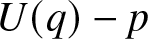 $U(q)-p$. As an alternative, this result can be derived from the probabilistic representation of the buffer size distribution as in [Reference Ingemar and Taisiia15, Corollary 1]. The resulting system is in a steady state with throughput
 $V_T(q^*) \lt p$ and loss probability given by
 $\mathbb{P}_{\text{loss}} = 1 - V_T(q^*)/p$. The loss probability specifically quantifies the likelihood of transmission failure for newly arrived signals. In contrast, the conventional outage probability is
 $1 - V_T(q^*)$, which represents the probability of transmission failure for an arbitrary signal, regardless of its origin. The no-loss system
 $K = \infty$, on the other hand, has
 $T^*_\mathrm{max}(p,w) \lt \infty$. The defining relation for
 $\{q_n\}$ with
 $q_0=p$ is
 $q_n=p/U(q_{n-1})$,
 $n\ge 1$, and
 $(p,w,t)$ is restricted to
 $t \lt T^*_\mathrm{max}(p,w)$, where there exists a minimal solution
 $q^*$ of the recursion
 $q_n=(p/V_t(q_{n-1}))q_{n-1}$, which satisfies the balance equation
 \begin{equation}
V_t(q^*)=p
\end{equation}
([Reference Ingemar and Taisiia15, Lemma 4]). The equilibrium buffer size in the no-loss model is the geometric distribution
 \begin{equation}
\pi_k=\frac{1-q^*}{1-p}\Big(1-\frac{1-q^*}{1-p}\Big)^k,\quad k\ge 0.
\end{equation}
We also observe that the reference case of pure loss,  $K=0$, has
 $B_n=0$ and
 $q_n=p$ for all
 $n$, hence
 $q^*=p$.
To complement the previous results, for maximum buffer size  $K$,
 $1\le K \lt \infty$, and given
 $(p,w,t)$, we let
 $q_K^*=q_K^*(p,w,t)$ be the minimal solution of the balance equation
 $q=F_K(q)$. It follows from (10) or (11) that
 $F_K$ increases in
 $K$; that is,
 $F_K(q)\le F_{K+1}(q)$,
 $0 \lt q \lt 1$. Moreover, we know that
 $p \lt F_K(q) \lt 1$ for each
 $q$,
 $p \lt q \lt 1$. Thus, the solutions
 $q_K^*=F_K(q_K^*)$ and
 $q_{K+1}^*=F_{K+1}(q_{K+1}^*)$ must satisfy
 $q_K^*\le q_{K+1}^*$, and we have the monotonicity in
 $K$, that is
 \begin{equation}
q_K^*\le q_{K+1}^*,\quad K\ge 1.
\end{equation}
Restricting to  $t \lt T^*_\mathrm{max}(p,w)$, these properties extend to
 $K=\infty$.
2.3. Coverage probability as a function of the  $\mbox{SINR}$ threshold

To further develop the approach described above, we state upper bounds for the coverage probability, which will ensure suitable integrability properties of  $\{V_t(q)\}_{t\ge 0}$. For convenience, we introduce the additional notation
 \begin{equation}
G_\delta(t)=
\int_1^\infty \frac{du}{1+(1+u^\delta)/t},\quad t \gt 0.
\end{equation}
Lemma 1. The family of downlink coverage probability functions  $V_t(q)$ in (5) for any
 $\sigma^2, \kappa \ge 0$ and
 $t\ge t_0 \gt 0$ satisfies the upper bound
 \begin{equation*}
V_t(q)\le \frac{q}{1+G_\delta\!(t_0)\,(t/t_0)^{1/\delta}\,qw }.
\end{equation*}
Proof. For downlink traffic with  $\sigma^2\ge 0$,
 $\kappa\ge 0$, using straightforward estimates in (5) and the auxiliary function
 $G_\delta(t)$ in (15),
 \begin{align*}
V_t(q) &\le \int_0^\infty q\, \exp\Big\{-v \int_1^\infty \frac{qw} {1+\frac{\kappa+v^\delta u^\delta}{t(\kappa +v^\delta)}}\,du\Big\}e^{-v}\,dv \nonumber \\
&\le \int_0^\infty q\, \exp\Big\{-v\int_1^\infty \frac{qw}
{1+(1+u^\delta)/t}\,du\Big\}e^{-v}\,dv
=\frac{q}{1+G_\delta\!(t)\, wq}.
\end{align*}
Moreover, using  $t\ge t_0$,
 \begin{equation}
G_\delta(t)=\int_1^\infty \frac{du}
{1+(1+u^\delta)/t}
= \int_{(t_0/t)^{1/\delta}}^\infty \frac{(t/t_0)^{1/\delta}\,du }
{1+1/t+u^\delta/t_0}
\ge G_\delta(t_0)\, (t/t_0)^{1/\delta},
\end{equation}
which gives the stated upper bound.
We note that in the simplest case when  $\kappa=0$ and
 $\sigma^2 = 0$, the coverage probabilities in (5) simplify considerably into the closed-form formula for downlink traffic
 \begin{equation}
V_T(q) = \frac{q}{1+H_\delta(T)\, w\,q},
\end{equation}
where
 \begin{equation}
H_\delta(t)=\int_1^\infty \frac{du}{1+u^\delta/t}
,\quad t \gt 0.
\end{equation}
As an example, the no-loss cellular downlink network with unbounded attenuation and no noise ( $K=\infty$,
 $\kappa=0$,
 $\sigma^2=0$), has a traffic distribution in equilibrium satisfying (12) if
 $p\le 1/(1+w\,H_\delta(T))$, in which case the probability of activity
 $q^*$ and the geometric buffer distribution
 $\pi$ in (13) are determined by
 \begin{equation}
q^*=\frac{p}{1-pw H_\delta(T)},\quad
\pi_0=\frac{1-p-pwH_\delta(T)}{(1-p)(1-pwH_\delta(T))}.
\end{equation}
3. Representation of the Shannon capacity
Here, we outline the definition of Shannon capacity for the buffered system under consideration, referring to [Reference Andrews, Baccelli and Ganti4] for the background and the interpretation of channel capacity in a comparable modeling situation. It should be emphasized that the resulting capacity expressions are not intended to represent an exact performance characterization of the interacting queuing system. Rather, they should be interpreted as analytical approximations that capture the average transmission capabilities of the wireless channel under the stochastic interference model.
Our goal is to determine a suitable region of admissible data rate-bandwidth pairs  $(p, w)$ to ensure that the system’s average transmission capacity is sufficient to accommodate the traffic intensity
 $pw$ in a steady-state regime. To achieve this, we relate the initial definition of coverage probability (6) with (9). By construction of (9), we have
 $\mathbb P(\mbox{SINR}_n \lt T^*_\mathrm{max}(p,w))=1$, and hence
 \begin{equation*}
V_T(q_n)=\mathbb P(T^*_\mathrm{max}(p,w) \gt \mbox{SINR}_n \gt T), \quad T \ge 0.
\end{equation*}
Then we associate with each time slot  $ n $ the (expected) Shannon capacity
 \begin{align*}
\mathbb E[w \log_2(1+\mathrm{SINR}_n)]
&= \frac{w}{\ln 2} \mathbb E\Big[\int_0^{\mathrm{SINR}_n} \frac{1}{1+t}\,dt\Big]\\
&= \frac{w}{\ln 2} \mathbb E\Big[\int_0^{T^*_\mathrm{max}(p,w)} \frac{\mathbf 1_{\{\mathrm{SINR}_n \gt t\}}} {1+t}\,dt\Big]
= \frac{w}{\ln 2} \int_0^{T^*_\mathrm{max}(p,w)}
\frac{V_t(q_n)}{1+t}\,dt, \quad n \ge 1,
\end{align*}
whenever the integral on the RHS exists finitely, and define the Shannon capacity  $\mbox{Cap}_K(p,w)$ for the
 $K$-buffer cellular network model as
 \begin{equation}
\mbox{Cap}_K(p,w)
=\lim_{n\to\infty} \frac{w}{\ln 2} \int_0^{T^*_\mathrm{max}(p,w)} \frac{V_t(q_n)}{1+t}\,dt,
\end{equation}
whenever this limit exists. In wireless communication theory, the quantity  $w\log_2(1+\mathrm{SINR})$ represents the instantaneously achievable transmission rate over a channel with bandwidth
 $w$ and signal-to-noise ratio SINR. In the model considered here, the SINR is a random variable, and the Shannon capacity defined in (20) therefore corresponds to the expected spectral efficiency of a typical link in the network. The integral representation in (20) is chosen so that the capacity can be expressed in terms of the coverage probabilities
 $V_t(q_n)=\mathbb{P}(\mathrm{SINR}_n \gt t)$. The upper integration limit
 $T^*_{\max}(p,w)$ is the maximal SINR threshold that can be reached in the network for the given traffic intensity and bandwidth parameters. Beyond this threshold, the system is unable to maintain successful transmissions, and consequently, the coverage probability becomes zero.
Before stating our first result on Shannon capacity, we highlight the key distinction between finite and infinite buffer networks. For any finite buffer size  $ 1\le K \lt \infty $, and given values of
 $ p $,
 $ w $, and
 $ t $, there exists a limit probability
 $q_n\to q^*=q^*(p,w,t) $, which represents the equilibrium probability that a typical transmitter is busy. The corresponding throughput satisfies
 $V_t(q^*) \lt p$, indicating that the system is always able to fully utilize the offered load. In contrast, for the infinite buffer system (
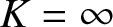 $ K = \infty $), the critical threshold
 $T^*_\mathrm{max}(p,w)$ is finite, such that, as long as
 $t \lt T^*_\mathrm{max}(p,w)$, there is a limit probability
 $q^*$, which ensures that the throughput reaches the offered load, in the sense
 $V_t(q^*)=p$.
From now on, the simpler notation  $T_\mathrm{max}(p,w)$ will denote the maximal critical transmission rate for the no-loss network,
 \begin{equation}
T_\mathrm{max}(p,w)=\sup\{t \gt 0:
V_t(q)=p\;\; \mbox{for some}\ q\in (p,1]\} \lt \infty.
\end{equation}
Hence, for  $K=\infty$,
 $T^*_\mathrm{max}(p,w)$ introduced in (9) coincides with
 $T_\mathrm{max}(p,w)$.
Theorem 3.1. For the various cases of the wireless network model, the expected Shannon capacity is finite,  $\mathrm{Cap}_K(p,w) \lt \infty$, and
i) for the pure-loss model  $K=0$,
 \begin{equation}
\mathrm{Cap}_0(p,w)
=\frac{w}{\ln 2} \int_0^\infty
\frac{V_t(p)}{1+t}\,dt,
\end{equation}
ii) for the loss and delay model with buffer size  $1\le K \lt \infty$,
 \begin{equation}
\mathrm{Cap}_K(p,w)=\frac{w}{\ln 2} \int_0^\infty
\frac{V_t(q^*_K(p,w,t))}{1+t}\,dt,
\end{equation}
iii) and for the no-loss model  $K=\infty$,
 \begin{equation}
\mathrm{Cap}_\infty(p,w)= wp \log_2(1+T_\mathrm{max}(p,w))
\end{equation}
with  $T_\mathrm{max}(p,w)$ defined in (21).
Proof. By Lemma 1 for downlink traffic,
 \begin{equation*}
V_t(q_n)\le \mathbf 1_{\{t\le t_0\}}
+ \frac{q_n}{1 + w \,G_\delta\!(t_0) (t/t_0)^{1/\delta}q_n}\mathbf 1_{\{t \gt t_0\}}.
\end{equation*}
Hence,  $V_t(q_n)\le g_\mathrm{down}(t)$, where
 \begin{equation*}
g_\mathrm{down}(t)= \mathbf 1_{\{t\le t_0\}}
+ \frac{1}{1 + w \,G_\delta\!(t_0) (t/t_0)^{1/\delta}}\mathbf 1_{\{t \gt t_0\}}, \quad t\ge 0.
\end{equation*}
The function  $g_\mathrm{down}$ is integrable, in the sense
 \begin{equation*}
\int_0^\infty \frac{g_\mathrm{down}(t)}{1+t}\,dt
=\ln(1+t_0)+\int_{t_0}^\infty \frac{1}{1 + w \,G_\delta\!(t_0) (t/t_0)^{1/\delta}} \frac{dt}{1+t} \lt \infty.
\end{equation*}
For the reference case i), it is now immediate from (2) and the definition (20) that  $\mathrm{Cap}_0(p,w) \lt \infty$, as for the case of no buffers we have
 $B_n=0$ and
 $q_n=p$ for all
 $n$.
For case ii), the limited loss network with buffers of maximal size  $K$,
 $1 \leq K \lt \infty$, we use the convergence
 $q_n\to q^* (p,w,t)$ and the continuity of the function in (5) to conclude that the integrand in (20) has the limit
 $V_t(q_n)\to V_t(q^*(p,w,t))$, as
 $n\to\infty$. The dominating function
 $g_\mathrm{down}$ for
 $V_t(q_n)$ are independent of
 $n$ and integrable with respect to
 $dt/(1+t)$. Now (23) follows by an application of the Lebesgue dominated convergence theorem.
Turning to the no-loss network iii) with  $K = \infty$,
 \begin{equation}
V_t(q_n)\nearrow V_t(q^*)=p,\quad t \lt T_\mathrm{max}(p,w).
\end{equation}
Therefore,
 \begin{align}
\mbox{Cap}_\infty(p,w)
&=\frac{w}{\ln 2} \int_0^{T_\mathrm{max}(p,w)}
\frac{V_t(q^*(p,t))}{1+t}\,dt \nonumber \\
&=\frac{pw}{\ln 2} \int_0^{T_\mathrm{max}(p,w)} \frac{dt}{1+t}
\nonumber\\
&= pw \log_2(1+T_\mathrm{max}(p,w)).
\end{align}
Part i) of the theorem is an extension of [Reference Andrews, Baccelli and Ganti4, Theorem 3], where the authors consider a pure loss, saturated downlink system with constantly active transmitters, normalized bandwidth, and the interference is Rayleigh fading. In our setting, this corresponds to the pure loss case  $K = 0$ with
 $\kappa=0$,
 $p=q=1$,
 $w=1$, and
 $\beta \gt d=2$, which means that the system always works at the highest activity level. For example, also assuming no-noise
 $\sigma^2=0$ and path loss coefficient
 $\beta=4$ in dimension
 $d=2$, so
 $\delta = 2$, it follows from (17) that
 \begin{equation*}
V_T(1) = \frac{1}{1 + \sqrt{T} (\pi/2 - \arctan(1/\sqrt{T}))},
\end{equation*}
and then (22) yields
 \begin{equation*}
\mathrm{Cap}_0(1,1)=\int_0^\infty \frac{V_t(1)}{1+t}\,dt
=\int_0^\infty \frac{1}{1 + \sqrt{e^t-1} (\pi/2 - \arctan(1/\sqrt{e^t-1}))}\,dt,
\end{equation*}
now measured in  $\mathrm{nats}=\ln 2 \,\,\mathrm{bits}$ per slot.
We make some further remarks on the interpretation of Theorem 3.1. In parallel to (6), for a given  $K\ge 1$, let
 $\mbox{SINR}^*$ be a random variable with
 $\mathbb P(\mbox{SINR}^*=0)=1-q^*_K (p,w,0)$ and
 $\mathbb P(\mbox{SINR}^* \gt t)=V_t(q^*_K(p,w,t))$. Then, for
 $K \lt \infty$,
 \begin{equation*}
\mbox{Cap}_K(p,w)=w\,\mathbb E[\log_2(1+\mbox{SINR}^*)].
\end{equation*}
In particular, the distribution of  $\mbox{SINR}^*$ for the case of the unbounded buffer network
 $K=\infty$, is simply given by
 $\mathbb P(\mbox{SINR}^*=0)=1-p$ and
 $\mathbb P(\mbox{SINR}^*=T_\mathrm{max}(p,w))=p$, which yields (24). As an additional comment, using the loss probability of a signal in our model, namely
 $P_\mathrm{loss}(p,w,t)=1-V_t(q^*(p,w),t)/p$, the Shannon capacity for
 $K \lt \infty$ has the representation
 \begin{equation*}
\mathrm{Cap}_K(p,w)=\frac{pw}{\ln 2} \int_0^\infty
\frac{1-P_\mathrm{loss}(p,w,t)} {1+t}\,dt.
\end{equation*}
Thus, at least indirectly, the loss rates distributed over a scheme of available SINR values determine the resulting capacity.
3.1. Admissible capacity regions
To relate the Shannon capacity more directly to the traffic handled by the network, we introduce a notion of admissible operating parameters. Intuitively, the system should be considered in working order whenever the average transmission capacity of the channel exceeds the traffic demand. To address overload, we apply the Shannon capacity to distinguish between two types of network states, specifically oversaturated and non-oversaturated systems, which represent “non-workable” and “workable” networks, respectively. This motivates the definition of a region of admissible data rate-bandwidth pairs.
Definition 3.2. A wireless system with buffer size  $K$, data rate
 $p$ and bandwidth
 $w$ is said to be capacity-admissible, if
 $(p,w)\in R_K$, where
 $R_K$ is the capacity-admissible region of data rate and bandwidth defined as
 \begin{equation}
R_K=\{(p,w): \mathrm{Cap}_K(p,w)\ge pw\}.
\end{equation}
From an engineering perspective, the capacity-admissible region  $R_K$ describes the set of operating parameters
 $(p,w)$ for which the wireless system is able to maintain the incoming traffic. The quantity
 $pw$ represents the average traffic demand per cell, while the Shannon capacity
 $Cap_K(p,w)$ characterizes the average transmission capacity of the channel in the presence of interference and retransmissions. The condition
 $Cap_K(p,w)\ge pw$ therefore identifies a regime such that the available transmission resources are sufficient to process the incoming signals without long-term overload of the buffers. Parameters outside this region correspond to an over-saturated system where the traffic demand exceeds the achievable capability. In other words, the system is capacity-admissible if, for fixed bandwidth, the data rate is small enough so that the capacity exceeds the external traffic intensity. Equivalently, for a fixed data rate, the condition (27) holds if the bandwidth is small enough for the traffic intensity to stay below the Shannon capacity. For example, for
 $K=\infty$ we see from (24) that the system is capacity-admissible if
 $\log_2(1 + T_\mathrm{max}(p, w)) \ge 1$, that is,
 $T_\mathrm{max}(p,w)\ge 1$.
3.1.1. Special case
$\kappa=\sigma^2=0$

Toexplicitly compute the capacity-admissible region, we consider the coverage probability in (17) for downlink traffic without noise and with unbounded attenuation, 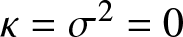 $\kappa=\sigma^2=0$. It is seen immediately in Theorem 3.1 i) that the Shannon capacity of the pure-loss system with
 $K=0$ is
 \begin{equation}
\mbox{Cap}_0(p,w) = \frac{pw}{\ln2} \int_0^{\infty} \frac{1}{1+H_\delta(t)\,w p}\frac{1}{1 + t}\,dt.
\end{equation}
The associated capacity-admissible region is
 \begin{equation}
R_0=\Big\{(p,w): \frac{pw}{\ln 2}\int_0^\infty \frac{1}{1+w p H_\delta(t)}\frac{1}{1+t}\,dt
\ge pw \Big\},
\end{equation}
which is the set  $\{(p,w): pw\le \alpha\}$, with
 $\alpha$ the constant determined by
 \begin{equation*}
\int_0^\infty \frac{1}{1+\alpha H_\delta(t)}\frac{1}{1+t}\,dt=\ln 2.
\end{equation*}
Turning to the other extrema case of the no-loss system  $K = \infty$, we noticed in (19) that the limiting busy-link probability
 $q_\infty^*(p,w,t)$ is
 \begin{equation*}
q_\infty^*(p,w,t)=\frac{p}{1-pw H_\delta(t)},\quad t \lt T_\mathrm{max}(p,w),
\end{equation*}
where  $T_\mathrm{max}(p,w)$ is such that
 $q_\infty^*(p,w,t) \le 1$. Hence, using (18),
 $T_\mathrm{max}(p,w)$ is the solution of the equation
 \begin{equation}
H_\delta(T_\mathrm{max}(p,w))
=\int_1^\infty \frac{1}{1+u^\delta/T_\mathrm{max}(p,w)}\,du=\frac{1}{w} \big(\frac{1}{p}-1\big).
\end{equation}
By Theorem 3.1 iii) and the Definition 3.2, the no-loss system is capacity-admissible if  $T_\mathrm{max}(p,w)\ge 1$, that is,
 $H_\delta(T_\mathrm{max}(p,w))\ge H_\delta(1)$, which implies that the capacity-admissible region is
 \begin{equation}
R_\infty =\Big\{(p,w): p \le
\frac{1}{1+w H_{\delta}(1)}\Big\}.
\end{equation}
In the opposite situation of  $T_\mathrm{max}(p,w) \lt 1$, the capacity of the no-loss system no longer covers the input rate intensity, in the sense made precise in Definition 3.2. A possible interpretation is degradation in delay and network performance to the extent that the system becomes non-workable.
To continue with finite buffer sizes  $K\ge 1$, by (14), since
 $V_T(q)$ in (17) is an increasing function of
 $q$, it follows that
 $\mathrm{Cap}_K(p,w)$ defined in (23) also is increasing in
 $K$. Thus, we have
 \begin{equation}
\mathrm{Cap}_0(p,w)\le\dots\le \mathrm{Cap}_K(p,w)\le \mathrm{Cap}_{K+1}(p,w)\le
\dots
\end{equation}
For  $K=1$ the probability
 $q^*_1$ can be found explicitly as a function of
 $p$,
 $w$, and
 $t$ by solving the balance equation (10). The capacity
 $\mathrm{Cap}_1(p,w)$ and the region of admissible traffic
 $R_1$ are then obtained from (23). In principle, analogous numerical results can be derived for any finite buffer size
 $K \geq 1$. However, both theoretical and numerical analyses are increasingly challenging due to the growing complexity of the solutions
 $q^*_K$, which in turn affects the resulting capacity function
 $\mathrm{Cap}_K(p, w)$. To address this shortcoming, we propose an alternative approach to studying the Shannon capacity. Instead of computing the capacity for a specific value of
 $K$, we derive an upper bound as a generic measure of the Shannon capacity valid for any
 $K \lt \infty$. For this, we use
 $T_\mathrm{max}(p,w)$ defined in (30) and split the Shannon capacity in Theorem 2, ii) into two parts:
 \begin{equation}
\mathrm{Cap}_K(p,w)
= \frac{w}{\ln 2}\Big( \int_0^{T_\mathrm{max}(p,w)}
\frac{V_t(q^*)}{1+t}\,dt +\int_{T_\mathrm{max}(p,w)}^\infty
\frac{V_t(q^*)}{1+t}\,dt\Big).
\end{equation}
Since  $V_t(q^*)\le p$, the first integral in (33) is bounded by the no-loss capacity
 $wp\log_2(1+ T_\mathrm{max}(p,w))$ obtained in (24). For the second integral, since the function
 $V_t(q)$ for the special case (17) is monotone in
 $q$, the inequality
 $V_t(q^*)\le V_t(1)$ yields
 \begin{equation}
\mathrm{Cap}_K(p,w)\le C(p,w),
\end{equation}
where
 \begin{equation}
C(p,w)=\frac{wp}{\ln 2}
\ln(1+T_\mathrm{max}(p,w)) +\frac{w}{\ln 2}\int_{T_\mathrm{max}(p,w)}^\infty
\frac{1}{1+H_\delta(t)w}\frac{1}{1+t}\,dt.
\end{equation}
Next, we define
 \begin{equation}
R =\{(p,w): C(p,w)\ge pw\}
\end{equation}
to be the region of data rate-bandwidth pairs that are admissible for the capacity upper bound  $C(p,w)$. Then it follows from (34) that the admissible regions
 $R_K$ are contained within the region admissible for the upper bound,
 $R_K\subset R$, for every finite
 $K$.
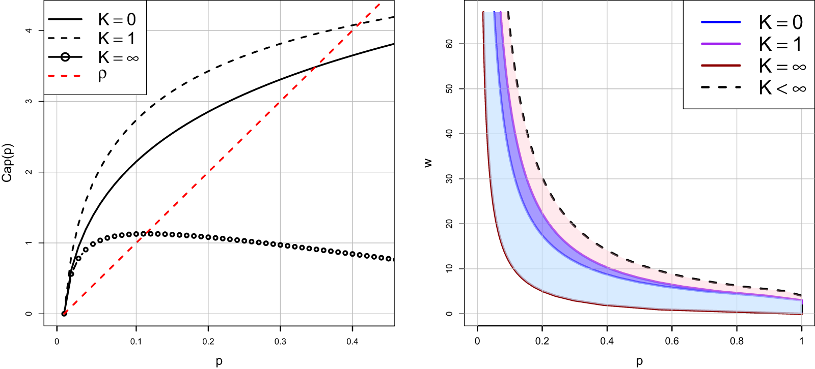
The numerical results are demonstrated in Figure 1, where plot (a) shows Shannon capacities  $\mathrm{Cap}_0(p,w), \mathrm{Cap}_1(p,w)$ and
 $\mathrm{Cap}_\infty(p,w)$ together with the traffic intensity
 $\rho = pw$ as functions of
 $p$ for the choice
 $\delta=2$ and
 $w=10$. The plot (b) shows the admissible regions for capacity (cases
 $K = 0, 1, \infty$) as well as the admissible region
 $R$ from (36) for the upper limit of capacity for general
 $K$. The contour set
 $\{(p,w): C(p,w)=pw\}$ for varying
 $p$ and
 $w$ is displayed as a dashed line. It follows from (32) that the admissible regions
 $R_K$ are increasing sets with increasing
 $K \lt \infty$.
Shannon capacity for different buffer sizes  $K$ and associated admissible regions. The parameters are
 $\kappa=0$,
 $\sigma^2=0$,
 $\delta=2$,
 $w=10$. Left panel (a): Shannon capacity
 $\mathrm{Cap}_K(p,10)$ for
 $K=0,1,\infty$, and traffic intensity
 $\rho=wp$. Right panel (b): The admissible regions
 $R_0$,
 $R_1$, and the set
 $R$ introduced in (36), as well as
 $R_\infty$, which for these parameters satisfy
 $R_\infty\subset R_0$.

1 Long description
Line graph with legend entries: K equals 0, K equals 1, K equals infinity and rho. The horizontal axis label is p, with tick labels 0, 0.1, 0.2, 0.3, 0.4. The vertical axis label is Cap(p), with tick labels 0, 1, 2, 3, 4. A solid curve labeled K equals 0 starts near (0, 0) and rises to about (0.1, 2.1), (0.2, 2.8), (0.3, 3.3) and about (0.45, 3.8). A dashed curve labeled K equals 1 starts near (0, 0) and rises above the solid curve to about (0.1, 2.7), (0.2, 3.5), (0.3, 3.9) and about (0.45, 4.3). A curve marked with open circle points labeled K equals infinity starts near (0, 0), rises to about (0.05, 1.0), reaches about (0.1, 1.1), stays near about 1.1 around p from 0.1 to 0.2, then decreases to about (0.3, 1.0) and about (0.45, 0.8). A dashed straight line labeled rho runs upward from near (0, 0) through about (0.1, 1.0), (0.2, 2.0), (0.3, 3.0) and about (0.45, 4.5). Plot with a horizontal axis label p and tick labels 0, 0.2, 0.4, 0.6, 0.8, 1 and a vertical axis label w with tick labels 0, 10, 20, 30, 40, 50, 60. The legend entries are K equals 0, K equals 1, K equals infinity and K less than infinity. Three filled regions are bounded by curves that decrease as p increases. The boundary curve for K equals infinity is the lowest, passing near about (0.1, 10), (0.2, 5), (0.4, 2), (0.6, 1.2), (0.8, 0.8) and (1, 0.6). The boundary curve for K equals 0 lies above it, passing near about (0.1, 20), (0.2, 12), (0.4, 6), (0.6, 4), (0.8, 3) and (1, 2.5). The boundary curve for K equals 1 lies above the K equals 0 curve, passing near about (0.1, 25), (0.2, 15), (0.4, 7), (0.6, 4.5), (0.8, 3.2) and (1, 2.7). A dashed curve labeled K less than infinity lies above the filled regions, passing near about (0.1, 35), (0.2, 20), (0.4, 10), (0.6, 7), (0.8, 5) and (1, 4).
3.1.2. General case
The observations discussed in the previous subsection demonstrate that pure loss and finite buffer networks possess a potential gain in capacity relative to no-loss networks in the scenario where  $\kappa = \sigma^2 = 0$. This increase arises from the fact that loss systems retain access to higher transmission rates at
 $t \geq T_{\mathrm{max}}(p, w)$. To briefly discuss the capacity behavior in a more general network, we keep
 $\kappa=0$ but allow
 $\sigma^2\ge 0$ in (5). The associated coverage probability
 $V_t^{(\sigma^2)}(q)$, which in this case also depends on the parameter
 $\mu$, satisfies
 $V_t^{(\sigma^2)}(q)\le V_t^{(0)}(q)$ for all
 $t \gt 0$ and
 $q$. Moreover, the maximum transmission rate is reduced,
 $T_\mathrm{max}^{(\sigma^2)}(p,w)\le T_\mathrm{max}^{(0)}(p,w)$ and therefore
 \begin{equation*}
\mbox{Cap}^{(\sigma^2)}_0(p,w)\le
\mbox{Cap}_0(p,w), \qquad
\mbox{Cap}^{(\sigma^2)}_\infty(p,w)\le
\mbox{Cap}_\infty(p,w).
\end{equation*}
4. Densification and frequency reuse
To continue the analysis of Shannon capacity in a new direction, we turn to the study of frequency reuse and network densification. Frequency reuse is a fundamental principle in cellular network design that enables efficient spectrum utilization by partitioning a network area into multiple cells ([Reference Ahaneku and Chijindau1]). Each cell is assigned a subset of the available frequency spectrum, which can be reused in cells that are not adjacent to minimize interference. This technique allows for a significant increase in network capacity by enabling multiple users to communicate simultaneously over the same frequency bands while maintaining an acceptable level of interference. A similar effect is achieved by employing network densification, where additional BSs are deployed to improve overall network performance and potentially increase channel capacity. Hence, the concept of both frequency reuse and densification is closely related to studies of the Shannon capacity measure, and, as a result, is of particular relevance to our analysis of the considered model.
The scaling analysis considered in this section is motivated by the design of dense cellular networks where the number of users and BSs increases over time. In the buffered system described in Section 2, such changes directly influence the traffic intensity per cell, the interference field, and the resulting queue dynamics. The analytical results obtained below therefore describe how the long-term throughput of the spatial queueing network evolves as system parameters such as bandwidth, user density, or frequency reuse are varied. In particular, the capacity limits derived in the following subsections correspond to performance regimes that would be observed in long-time simulations of the underlying stochastic network. From an engineering perspective, increasing the density of users or BSs initially improves the average transmission capability of the network by providing more transmission opportunities and more efficient spatial reuse. This improvement appears in our analysis as an increase in the Shannon capacity for larger buffer sizes. However, as densification continues, interference between simultaneously active transmitters becomes more significant and the achievable SINR levels decrease, which limits further gains. As a result, the capacity improvements obtained through densification eventually saturate and reach their limits.
4.1. Frequency reuse
To meet realistic coverage targets with a sufficiently high probability, it is common to apply frequency-reuse methods. In this approach, the reuse factor  $k\ge 1$ is the number of frequency bands available in the network. The higher the number of frequency bands, the lower the number of cells that share the same frequency ([Reference Andrews, Baccelli and Ganti4]). Since each BS can pick one of
 $k$ different frequency bands, the interference field is reduced and now only occurs between the BSs that use the same frequency. Therefore, a simplified approach to implement frequency reuse is to reduce the bandwidth from
 $w$ to
 $w/k$, and hence obtain the relevant performance measures under frequency reuse as functions of
 $k$. For the pure-loss case, using (22), we implement the capacity frequency reuse as
 \begin{equation*}
\mathrm{Cap}_0(p,w/k)
= \frac{1}{\ln2} \int_0^{\infty}\frac{wp} {(k+H_\delta(t)\,wp)(1 + t)}\,dt.
\end{equation*}
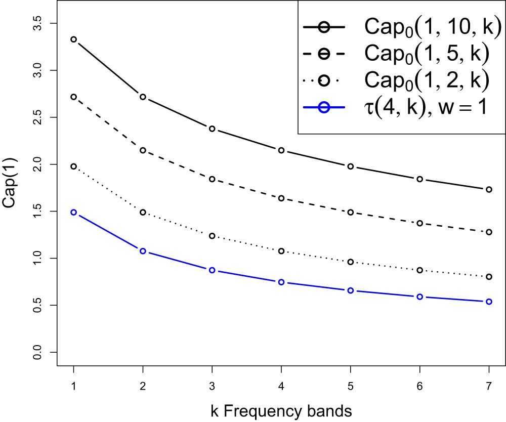
We see that the above function decreases with increasing reuse factor  $k$, and vanishes in the limit as
 $k\to\infty$. This is again consistent with the results presented in [Reference Andrews, Baccelli and Ganti4] in which a normalization
 $w=1$ applies. The function
 $\tau(4,k)$ in [Reference Andrews, Baccelli and Ganti4] is the same as our
 $\mathrm{Cap}_0(1,1/k)$ for
 $\delta=2$, compare Figure 2.
Comparison of the Shannon capacity  $Cap_0(1, w/k)$ for different bandwidths
 $w$ with
 $\tau(4, k)$ in [Reference Andrews, Baccelli and Ganti4, VI.B], as a function of the reuse factor
 $k$.

4.2. Densification
Earlier work on the performance analysis of wireless pure-loss systems also considered limit schemes in the opposite direction of increasing bandwidth. This is a densification setting, widely used in modern communication systems in light of ultra-dense 5G networks designed to handle vast amounts of data from a large number of users ([Reference Bhushan, Junyi, Malladi, Gilmore, Brenner, Damnjanovic, Sukhavasi, Patel and Geirhofer7]). In terms of our model, the increase in traffic demand can be implemented by letting the number of users per cell grow,  $\lambda_0\to\infty$, formalized as the limit relation
 $w=\lambda_0/\lambda_1 \to \infty$. In [Reference AlAmmouri, Andrews and Baccelli2, Theorem 1], under assumptions related to our pure-loss model, the authors study the expected average rate and obtain in the many-user limit the existence of a densification plateau, in practice a saturation limit of performance. In parallel, we obtain a similar capacity limit as the user density increases. By (23),
 \begin{align}
\mathrm{Cap}_0&(p, \infty) :=
\lim_{w \to \infty} \mathrm{Cap}_0(p, w) \nonumber \\
&=\frac{1}{\ln2} \int_0^\infty \lim_{w \to \infty}
\frac{wp} {(1+H_\delta(t)\,wp)(1 + t)}\,dt \nonumber \\
&= \frac{1}{\ln2} \int_0^{\infty}
\frac{dt}{H_\delta(t)(1 + t)} \lt \infty,
\end{align}
where we use dominated convergence to perform the limit-integral interchange. It is noted that the limit does not depend on the individual data rate  $p$.
To extend the analysis beyond the model investigated in [Reference AlAmmouri, Andrews and Baccelli2], we consider the same limit of densification for the no-loss system. Using (24) for  $K = \infty$ we compute the limiting capacity
 \begin{equation}
\mathrm{Cap}_{\infty}(p, \infty) :=
\lim_{w\to\infty} wp \log_2(1 + T_\mathrm{max}(p,w)),
\end{equation}
recalling from (30) that  $T_\mathrm{max} := T_\mathrm{max}(p,w)$ is the unique solution of
 \begin{equation*}
H_\delta(T_\mathrm{max})=(1-p)/pw.
\end{equation*}
Using this relation, it first follows that  $T_\mathrm{max} \to 0$ as
 $w\to\infty$ for a fixed
 $p$. Moreover, in this limit,
 \begin{equation*}
w\,T_\mathrm{max} = \frac{1 - p}{p} \frac{T_\mathrm{max}}{H_\delta(T_\mathrm{max})}
=\frac{1 - p}{p} \Big(\int_1^{\infty} \frac{du}{T_\mathrm{max} + u^{\delta}}\Big)^{-1} \to
\frac{(1 - p)(\delta-1)}{p}.
\end{equation*}
By expanding the logarithm in (38) this yields
 \begin{equation}
\mathrm{Cap}_{\infty}(p, \infty) =\frac{(1 - p)(\delta-1)}{\ln 2}.
\end{equation}
Furthermore, it can be checked for  $K=1$ that
 $\mathrm{Cap}_1(p, \infty)$ coincides with the limit obtained in (37). As a consequence, by (34) and (35), for any
 $K$,
 \begin{equation*}
\frac{1}{\ln2} \int_0^{\infty}
\frac{dt}{H_\delta(t)(1 + t)}
\le \mathrm{Cap}_K(p, \infty)
\le C(p, \infty)
= \frac{(1 - p)(\delta-1)}{\ln 2}
+\frac{1}{\ln2} \int_0^{\infty}
\frac{dt}{H_\delta(t)(1 + t)},
\end{equation*}
where  $C(p, \infty) = \lim_{w \to \infty} C(p, w)$ with
 $C(p,w)$ defined in (35). The limit result for the system with an unlimited buffer may seem counterintuitive. On the one hand, network densification forces the admissible maximal SINR threshold
 $T_\mathrm{max}$ to approach zero, indicating that the network cannot handle increasing traffic demand, but on the other hand, network performance improves as the average capacity reaches the plateau level in (39). To clarify, we let
 $p_\mathrm{max}$ be the maximal
 $p$, such that
 $(p,w)$ belongs to
 $R_\infty$, defined in (31). We then note that
 $p_\mathrm{max}$ also tends to zero as
 $w \to \infty$. The limiting network state, therefore, lies outside the admissible region
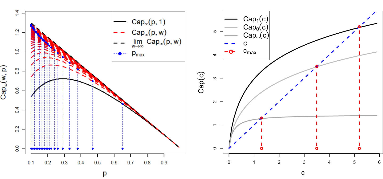
 $R_\infty$. Figure 3(a) illustrates the effect of densification on the no-loss capacity. The plot shows
 $\mathrm{Cap}_\infty(p,w)$ for increasing values of
 $w$ (dashed red lines), beginning from
 $w = 1$ (black line). For each
 $w$, the maximum rate
 $p_\mathrm{max}$ is displayed with dashed blue lines. The plot shows that the critical threshold
 $p_\mathrm{max}$ approaches
 $1$ when the limiting capacity approaches
 $0$, which is natural and consistent with the previous discussion.
Capacity limits in different representations for  $\delta=2$. (a) Convergence of the channel capacity
 $\mathrm{Cap}_\infty(p,w)$ as
 $w \to \infty$, starting from
 $w = 1$ (solid black line). The capacity increases for larger
 $w$, leading to
 $p_{max}$ approaching zero. (b) Capacity limit as a function of
 $c$ for
 $K = 0, K = 1$, and
 $K = \infty$.

Figure 3 Long description
A) Left plot with x-axis label p, ranging from 0.1 to 0.9 with ticks at 0.1 intervals. The y-axis label is Cap infinity (w, p), ranging from 0.0 to 1.4 with ticks at 0.2 intervals. A legend lists: Cap infinity (p, 1) as a solid line; Cap infinity (p, w) as dashed lines; lim w arrow infinity Cap infinity (p, w) as a dashed line; and p max as dotted markers with vertical dashed guide lines. The solid curve starts near about 0.55 at p equals 0.1, rises to a broad peak near about 0.7 around p between 0.25 and 0.35, then decreases, reaching about 0.5 near p equals 0.6 and approaching 0 near p equals 0.9. Multiple dashed curves form a band above the solid curve, with values near about 1.3 around p equals 0.1 and decreasing roughly linearly toward 0 as p approaches 0.9. A dashed limiting curve follows the upper envelope and also trends down to 0 near p equals 0.9. Along the bottom, dotted markers indicate p max positions and many vertical dashed guide lines rise from these markers up into the plot. B) Right plot with x-axis label c, ranging from 0 to 6 with ticks at 1 intervals. The y-axis label is Cap (c), ranging from 0 to 6 with ticks at 1 intervals. The legend lists Cap 1 (c), Cap 0 (c), Cap infinity (c), c and c max. Three smooth curves start near 0 at c equals 0 and increase with c. The top curve rises steeply at small c and then bends toward a plateau, reaching a little above 5 at c near 5 and about 5.4 near c equals 6. A middle curve increases more slowly, reaching about 4.0 near c equals 6. A lower curve increases and then flattens near about 1.4 by c around 2 to 6. A diagonal dashed line labeled c runs from near (0, 0) upward to near (6, 6). Three vertical dashed lines labeled c max are drawn at approximately c equals 1.3, c equals 3.4 and c equals 5.2, each with a circular marker at the top where it meets the top curve and a circular marker near the bottom on the x-axis.
4.3. Shannon capacity under balanced densification
In this section, we propose a new approach to studying capacity performance under densification. To better understand the limiting effects discussed in previous subsections, we also consider a balanced densification regime in which the bandwidth (or equivalently the number of users per cell) increases while the input rate per transmitter decreases in such a way that the overall traffic intensity remains constant. In this scaling limit, the capacity approaches a well-defined limit, and the analysis reveals a maximal throughput level. Such a scaling is motivated by dense cellular networks where the number of connected devices grows, while the traffic generated by each device is typically smaller. In this situation, the total load per cell may remain approximately constant even as the number of users increases. To exemplify, we restrict the analysis to the case  $\kappa=\sigma^2=0$, for which the coverage probability is given by (17).
Mathematically, we consider the joint convergence of increasing bandwidth  $w$ and decreasing data rate
 $p$, such that the system has a limiting traffic intensity
 $c \gt 0$, in the sense of
 \begin{equation}
wp\to c,\quad w\to \infty, \quad p\to 0.
\end{equation}
For convenience, we implement the limit procedure by setting  $p = c/w$ and allowing
 $w \to \infty$. It is easy to see that the maximal transmission rate sequence
 $T_{\mathrm{max}}(c/w,w)$ in (30) is non-decreasing in
 $w$. The limit, denoted as
 \begin{equation*}
T_{\mathrm{max}}(c) = \lim_{w\to\infty} T_{\mathrm{max}}(c/w,w),
\end{equation*}
is the solution to the equation
 \begin{equation}
H_\delta(T_{\mathrm{max}}(c)) = 1/c.
\end{equation}
Next, we define the limiting capacity under balanced densification for  $0 \leq K \leq \infty$, again with some abuse of notation, as
 \begin{equation}
\mathrm{Cap}_K(c) = \lim_{w\to\infty} \mathrm{Cap}_K(c/w,w),
\end{equation}
provided the relevant limit exists. Analogously to Definition 3.2, we say that the traffic intensity  $c$ falls within the balanced Shannon capacity if
 $c \in I_K = [0, c_{\mathrm{max}}]$, where
 \begin{equation}
I_K = \{c \gt 0 : \mathrm{Cap}_K(c) \geq c \},
\end{equation}
denotes the admissible interval of traffic intensities supported within the balanced Shannon capacity. The upper bound  $c_{\mathrm{max}}$ of this interval is the maximum throughput that can be sustained by the maximum average rate
 $T_{\mathrm{max}}(c)$, which therefore theoretically could be transmitted in the network.
Theorem 4.1. Under the assumption of balanced densification (40), the limiting Shannon capacity  $\mathrm{Cap}_K(c)$ and the maximal admissible intensity
 $c_\mathrm{max}$ are
i) for the pure-loss model  $K=0$,
 \begin{equation*}
\mathrm{Cap}_0(c) = \frac{1}{\ln 2} \int_0^\infty \frac{c}{1 + c H_{\delta}(t)}\frac{dt}{1 + t},
\end{equation*}
with  $c_\mathrm{max}$ the unique solution of
 \begin{equation*}
\frac{1}{\ln 2}\int_0^\infty \frac{1}{1 + c_\mathrm{max} H_{\delta}(t)}\frac{dt}{1 + t}=1;
\end{equation*}
ii) for the loss and delay models with any finite buffer size  $K\ge 1$,
 \begin{equation*}
\mathrm{Cap}_K(c) = c\,\log_2\big( 1 + T_\mathrm{max}(c) \big) + \frac{1}{\ln 2} \int_{T_\mathrm{max}(c)}^{\infty} \frac{dt}{H_{\delta}(t)(1 + t)} ,
\end{equation*}
with  $c_\mathrm{max}$ the solution
 $c$ of
 \begin{equation*}
\log_2\big( 1 + T_\mathrm{max}(c) \big) + \frac{1}{c\,\ln 2} \int_{T_\mathrm{max}(c)}^{\infty} \frac{dt}{H_{\delta}(t)(1 + t)}=1;
\end{equation*}
iii) and for the no-loss model  $K=\infty$,
 \begin{equation}
\mathrm{Cap}_{\infty}(c) = c\,\log_2\big( 1 + T_\mathrm{max}(c) \big),
\end{equation}
with  $c_\mathrm{max}=1/H_\delta(1)$.
Proof. In the pure-loss case,  $\mathrm{Cap}_0(c/w,w)$ derived in (28) does not depend on
 $w$ and we obtain immediately
 \begin{equation}
\mathrm{Cap}_0(c)=\frac{1}{\ln2} \int_0^\infty
\frac{c} {(1+H_\delta(t)\,c)(1 + t)}\, dt.
\end{equation}
By Definition 3.2, the limiting traffic intensity  $c$ is within balanced Shannon capacity whenever
 $\mathrm{Cap}_{0}(c) \geq c$. Hence, as stated,
 $c_\mathrm{max}$ is the solution of
 $\mathrm{Cap}_0(c) = c$. Turning to case ii), finite maximal buffer size
 $1\le K \lt \infty$, we first observe that the scaled coverage probability for any
 $K$ has the upper bound
 \begin{equation*}
V_t\left(q^*\left(\frac{c}{w},w,t \right)\right)\le \frac{c}{w} \cdot \mathbf 1_{\{t \lt T_\mathrm{max}(c)\}}
+ \frac{\mathbf 1_{\{t \gt T_\mathrm{max}(c)\}}}{1+wH_\delta(t)}.
\end{equation*}
Hence  $wV_t(q^*(c/w,w,t))$ has the dominating function
 \begin{equation}
wV_t(q^*(c/w,w,t))
\le c \cdot \mathbf 1_{\{t \lt T_\mathrm{max}(c)\}}
+ \frac{\mathbf 1_{\{t \gt T_\mathrm{max}(c)\}}}{H_\delta(t)},
\end{equation}
which is independent of  $w$ and integrable in
 $t$, such that
 \begin{equation*}
\int_0^\infty \Big(c \cdot \mathbf 1_{\{t \lt T_\mathrm{max}(c)\}}
+ \frac{1}{H_\delta(t)}\cdot \mathbf 1_{\{t \gt T_\mathrm{max}(c)\}}\Big)\frac{dt}{1+t} \lt \infty.
\end{equation*}
Thus,
 \begin{equation}
\mathrm{Cap}_K(c) =\frac{1}{\ln 2} \int_0^\infty \lim_{w\to\infty} wV_t(q^*(c/w,w,t)) \frac{dt}{1+t}.
\end{equation}
Moreover, it follows from (46),(47) that
 \begin{equation}
\mathrm{Cap}_K(c) \le
\frac{c}{\ln 2}\int_0^{T_\mathrm{max}(c)} \frac{dt}{1+t}+\frac{1}{\ln 2}\int_{T_\mathrm{max}(c)}^\infty \frac{1}{H_\delta(t)}\frac{dt}{1+t}.
\end{equation}
Now we return to the explicit result for  $K=1$ mentioned in Section 3.1. The defining relation for
 $q^* = q^*(p,w,t)$ is found by solving (10) with
 $K = 1$, and is obtained explicitly as
 \begin{equation*}
q^*=\frac{\sqrt{(1-w H_\delta(t) p)^2+4w H_\delta(t) p^2}-(1-w H_\delta(t) p)}{2w H_\delta(t) p}.
\end{equation*}
For this case
 \begin{equation*}
\mathrm{Cap}_1(c/w,w)\cdot \ln 2 =
\int_0^\infty \frac{1+cH_\delta(t)-\sqrt{(1-cH_\delta(t))^2+4c^2 H_\delta(t)/w} }{2H_\delta(t)(1-c/w) }\frac{dt}{1+t}.
\end{equation*}
By (47),
 \begin{align*}
\mathrm{Cap}_1(c) &=
\frac{1}{\ln 2} \int_0^\infty \frac{1+cH_\delta(t)-|1-cH_\delta(t)|} {2H_\delta(t)}\frac{dt}{1+t}\\
&= \frac{1}{\ln 2}\int_0^\infty
c\cdot \mathbf 1_{\{cH_\delta(t) \lt 1\}} +\frac{1}{H_\delta(t)} \mathbf 1_{\{cH_\delta(t) \gt 1\}} \, \frac{dt}{1+t}.
\end{align*}
Now,  $cH_\delta(t) \lt 1$ iff
 $t \lt T_\mathrm{max}(c)$ and, therefore, the derived expression for
 $\mathrm{Cap}_1(c)$ coincides with the upper bound of
 $\mathrm{Cap}_K(c)$ in (48). The conclusion is that all capacities
 $\mathrm{Cap}_K(c)$ for finite
 $K\ge 1$ are equal. The corresponding
 $c_{max}$ can be read as stated in claim ii).
Finally, for the no-loss system iii), we have
 \begin{equation*}
\mathrm{Cap}_{\infty}(c/w,w) = c \log_2(1 + T_\mathrm{max}(c/w,w)).
\end{equation*}
By monotone convergence,  $\mathrm{Cap}_{\infty}(c/w,w) \to c \log_2(1 + T_\mathrm{max}(c))$ as
 $w \to \infty$. In this case, the maximum admissible intensity
 $c_{max}$ is obtained by solving
 $c \log_2(1 + T_\mathrm{max}(c)) = c$, or equivalently,
 $T_\mathrm{max}(c) = 1$. Then it follows from (41) that
 $c_\mathrm{max} = 1/H_{\delta}(1)$.
The results presented in this section demonstrate that channel capacity remains an informative performance measure in the balanced scaling regime of small input rate and large UE density. In particular, channel capacity is an explicit, relatively simple, increasing function of scaled traffic intensity  $c$. A new aspect of the analysis is that, under balanced densification, the retransmission mechanism does not influence the channel capacity when the buffer size
 $K$ is finite. Thus, physically, irrespective of the coding scheme employed, the channel capacity remains consistent, distinguishing only between systems with no buffer, a finite buffer, and an infinite buffer. An additional conclusion from Theorem 4.1 is that only scaled traffic intensities within the admissible intervals
 $[0, c_\mathrm{max}]$ are covered by the balanced Shannon capacity, expressed as
 \begin{equation*}
\mathrm{Cap}_K(c) \geq c.
\end{equation*}
As  $c$ grows larger, the channel capacities approach asymptotic plateau values in the limit
 $c \to \infty$, given by
 \begin{equation}
\lim_{c\to\infty}\mathrm{Cap}_K(c)
=\frac{1}{\ln2}\Big((\delta-1)\mathbf 1_{\{1\le K\le \infty\}} +\int_0^\infty
\frac{1}{H_\delta(t)} \frac{dt}{1 + t} \,\mathbf 1_{\{0\le K \lt \infty\}}\Big).
\end{equation}
Figure 3(b) illustrates the three cases of channel capacity limits under balanced densification obtained in Theorem 4.1, for  $K=0$, finite
 $K\geq 1$, and
 $K=\infty$. The limit functions shown in the figure indicate that an increase in bandwidth combined with a reduction in input rate leads to an improvement in scaled capacity up to a certain threshold. Beyond this threshold, any further increase in
 $c$ no longer improves network performance. The dashed red lines represent the maximum values
 $c_\mathrm{max}$ for each type of network (finite buffer, infinite buffer, and no buffer). The interpretation of these values is similar to the capacity-admissible regions introduced in Definition 3.2. That is, the system is deemed workable whenever
 $c \le c_\mathrm{max}$, and non-workable otherwise.
Competing interests
The authors have no competing interests to declare.






 Open access

