1 Introduction
Spherical bodies are often used as an approximation in modelling irregularly shaped particles in particle-laden flows (Elghobashi Reference Elghobashi1994) and can also be considered as the prototype of bluff bodies commonly encountered in man-made structures. However, as a result of the inherent three-dimensionality of the flow field, there is a lack of fully resolved, quantitative measurements of the wake of the sphere while undergoing vortex shedding, and the majority of quantitative three-dimensional (3-D) flow field characteristics in the sphere wake at low Reynolds numbers (
 ${<}1000$
) have come from numerical simulations (e.g. Johnson & Patel Reference Johnson and Patel1999; Ploumhans et al.
Reference Ploumhans, Winckelmans, Salmon, Leonard and Warren2002; Yun, Kim & Choi Reference Yun, Kim and Choi2006).
Many have studied the 3-D flow structure in the wake of spheres using dye or smoke visualizations (Möller Reference Möller1938; Achenbach Reference Achenbach1974; Sakamoto & Haniu Reference Sakamoto and Haniu1990; Leweke et al.
Reference Leweke, Provansal, Ormieres and Lebescond1999; Chrust, Goujon-Durand & Wesfreid Reference Chrust, Goujon-Durand and Wesfreid2013). Experiments were performed by either towing the sphere in a quiescent bath (Taneda Reference Taneda1956; Wu & Faeth Reference Wu and Faeth1993), or by imposing a uniform, upstream air velocity (Achenbach Reference Achenbach1974; Sakamoto & Haniu Reference Sakamoto and Haniu1990). All studies found that the wake flow topology strongly depended on the Reynolds number,
 $Re=UD/\unicode[STIX]{x1D708}$
, where
 $U$
is the relative velocity between the sphere and the upstream fluid (in the present study,
 $U$
is the bulk flow velocity),
 $D$
the sphere diameter and
 $\unicode[STIX]{x1D708}$
the kinematic viscosity. At
 $Re=24$
, a steady recirculating wake begins to form at the rear of the sphere, its length linearly increasing with
 $\ln (Re)$
until oscillations begin at
 $Re=130$
, leading to a wave-like undulating wake (Taneda Reference Taneda1956). The onset of vortex shedding occurs at
 $Re\approx 270$
(Johnson & Patel Reference Johnson and Patel1999; Ghidersa & Dušek Reference Ghidersa and Dušek2000), and hairpin shaped vortices are periodically shed in a highly regular pattern in the range
 $270<Re<420$
(Sakamoto & Haniu Reference Sakamoto and Haniu1990). Beyond this range, shedding becomes less regular and when
 $Re$
exceeds 800, the large-scale hairpin vortices break apart and two shedding frequencies are observed, the lowest associated with the large-scale sphere shedding, and the highest with the small scales that appear as a result of shear layer instabilities (Kim & Durbin Reference Kim and Durbin1988; Sakamoto & Haniu Reference Sakamoto and Haniu1990). All the visualization studies (
 $270<Re<420$
) revealed shedding as a ‘train’ of hairpin vortices having the same orientation. However, the direct numerical simulations (DNS) by Johnson & Patel (Reference Johnson and Patel1999) at
 $Re=300$
challenged this paradigm and showed that previously unidentified, oppositely oriented, secondary (‘induced’) hairpin vortices (never observed in visualization studies) were also shed from the sphere. Johnson & Patel (Reference Johnson and Patel1999) showed that the secondary vortices resulted from the interaction between the wake flow and the outer flow. The results by Johnson & Patel (Reference Johnson and Patel1999) were later corroborated by the DNS of Ploumhans et al. (Reference Ploumhans, Winckelmans, Salmon, Leonard and Warren2002) who also showed the existence of secondary hairpin vortices at
 $Re=300$
.
In contrast to the numerical studies, fully resolved, quantitative three-dimensional (3-D) experimental data of the sphere wake are sorely lacking. Brücker (Reference Brücker2001) performed a spatio-temporal reconstruction of the 3-D wake structure based on time-resolved particle image velocimetry (TR-PIV) in a two-dimensional (2-D) transverse plane positioned three diameters downstream of the sphere centre at
 $Re=400$
, 500 and 700. He found evidence for the existence of secondary vortices at
 $Re=400$
and 500. At higher Reynolds numbers, Doh, Hwang & Saga (Reference Doh, Hwang and Saga2004) and Jang & Lee (Reference Jang and Lee2008), investigated the flow in the wake of a stationary sphere using 3-D particle tracking velocimetry (PTV,
 $Re=1130$
) and planar PIV (
 $Re=11\,000$
), respectively. Recently, Terra, Sciacchitano & Scarano (Reference Terra, Sciacchitano and Scarano2017) and van Hout et al. (Reference van Hout, Eisma, Elsinga and Westerweel2018a
) used tomographic particle image velocimetry (tomo-PIV) to measure the flow in the wake of a sphere in uniform flow (
 $Re=10\,000$
) and immersed in a turbulent boundary layer (
 $692<Re<959$
), respectively. In the latter case,
 $Re$
was based on the undisturbed mean velocity in the turbulent boundary layer at the wall-normal centre position of the sphere. Terra et al. (Reference Terra, Sciacchitano and Scarano2017) used the measurements to estimate the drag force acting on the sphere while van Hout et al. (Reference van Hout, Eisma, Elsinga and Westerweel2018a
) showed that wall proximity caused preferential alignment of shed vortices resulting in a wall-directed (negative) lift force.
As far as the authors are aware, no spatially resolved, 3-D measurements have been reported in the literature to verify the occurrence of the secondary vortices reported in the DNS studies but never seen in dye and smoke visualizations. The goal of the present experiments is to reveal the fully resolved 3-D topology of the vortex shedding in the wake of a sphere immersed in a uniform flow at
 $Re=465$
. In particular, the occurrence of secondary vortices and their generation are investigated. In § 2 the experimental set-up including the tomo-PIV system is described. Section 3 discusses the data processing and the vortex shedding characteristics are illustrated in § 4. A summary and discussion is provided in § 5.
2 Experimental set-up
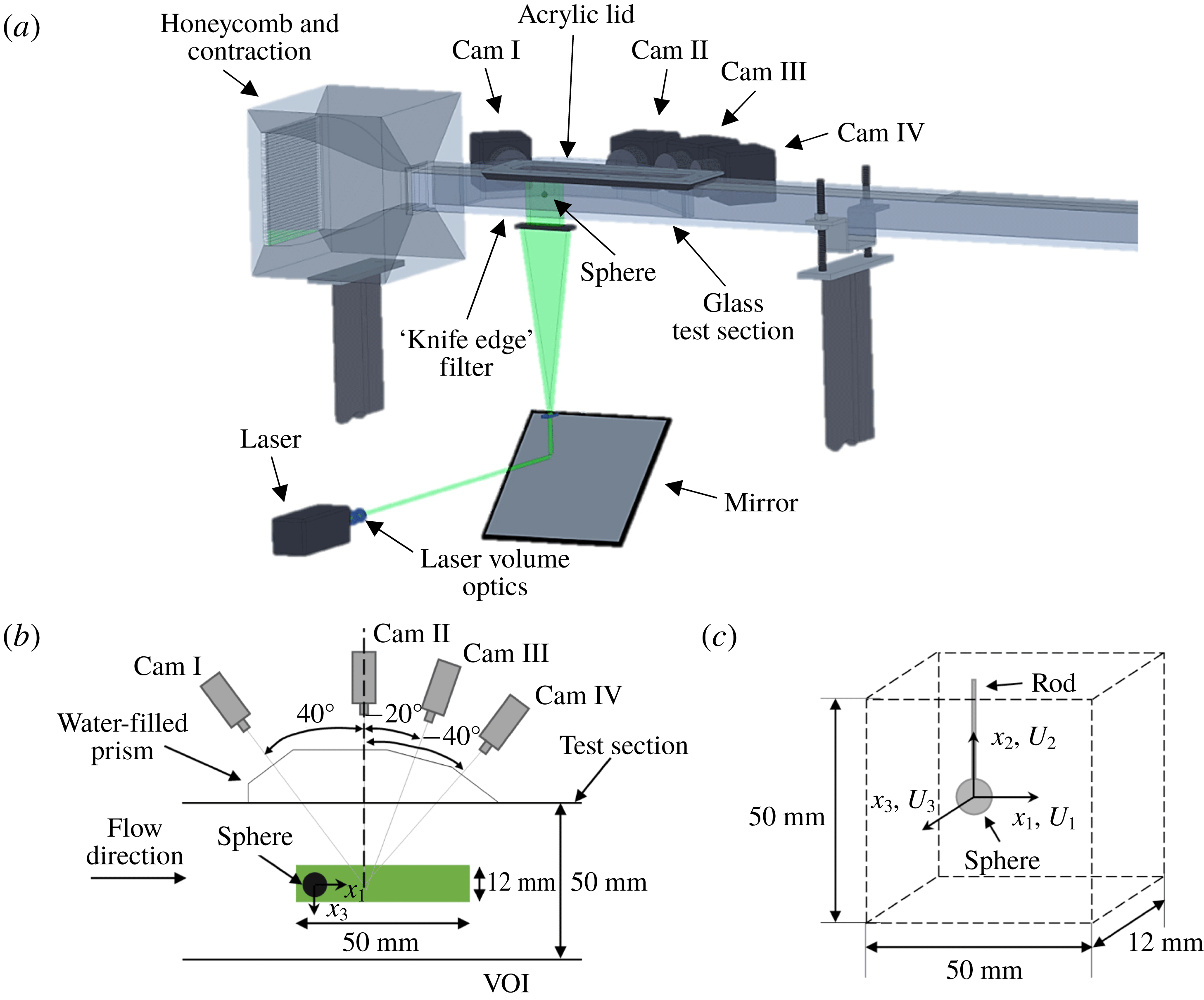
Experiments were performed in a closed-loop water tunnel (figure 1
a) comprising a centrifugal pump, magnetic flow meter, plenum, honeycomb flow straightener, contraction (9 : 1) and glass test section to ensure optical access from all sides. The square test section had an internal cross-section of
 $50\times 50~\text{mm}^{2}$
, and a total length of 2 m. Access into the test section from above was provided by an internally flush-mounted acrylic lid. The frequency controlled centrifugal pump was used to achieve bulk flow velocities in the range
 $0.03~\text{m}~\text{s}^{-1}<U<1.00~\text{m}~\text{s}^{-1}$
. For a more detailed description of the experimental facility the reader is referred to van Hout, Krakovich & Gottlieb (Reference van Hout, Krakovich and Gottlieb2010) and Eshbal, Krakovich & van Hout (Reference Eshbal, Krakovich and van Hout2012). A steel sphere of diameter
 $D=7.94\pm 0.01$
mm was mounted rigidly 14 cm downstream of the inlet to the test section by means of a vertical steel rod (diameter
 $d=0.75\pm 0.01$
mm, length
 $L=21.06\pm 0.01$
mm) attached to the acrylic lid. The ratio between the rod diameter and the sphere diameter,
 $d/D=0.094$
, was chosen to limit the effect of the rod on the sphere’s wake and prevent vibrations.
Schematic layout of (a) the tomo-PIV system, (b) the test section (top view) and (c) the volume of interest (VOI) and coordinate system.

The three-dimensional velocity field in the wake of the sphere was measured using tomo-PIV (Elsinga et al.
Reference Elsinga, Scarano, Wieneke and Van Oudheusden2006; Scarano Reference Scarano2013). The system (LaVision GmbH) consisted of four cameras (Imager Pro 4M,
 $2048\times 2048$
pixels), an Nd:YAG laser (Quantel 532 nm, max. 120 mJ at 15 Hz), laser volume optics and water filled prisms (figure 1) to limit the effects of refraction (Prasad Reference Prasad2000). Cameras I to IV were positioned in a horizontal plane (‘line setup’, Adrian & Westerweel Reference Adrian and Westerweel2011; Scarano Reference Scarano2013) at angles of
 $40^{\circ }$
,
 $0^{\circ }$
,
 $-20^{\circ }$
and
 $-40^{\circ }$
, relative to a line perpendicular to the flow direction (figure 1
b). Cameras were equipped with 50 mm lenses (Nikon, f-number: 22) including Scheimpflug adapters that were used to achieve focus across the image (Prasad Reference Prasad2000). The laser beam was expanded into a collimated beam having a rectangle cross-section of approximately
 $50\times 12~\text{mm}^{2}$
, using several plano-cylindrical lenses (5X and 8X magnification in perpendicular directions). In order to ensure sharp edges of the illuminated volume, the collimated beam was passed through a ‘knife-edge’ filter before entering the test section. The volume of interest (VOI) was approximately
 $50\times 50\times 12~\text{mm}^{3}$
and included the sphere (figure 1
c). Initial calibration was performed using a dual-plane calibration plate (LaVision, Type 22) that was mounted on a microstage (Thorlabs,
 $\pm 0.01$
mm) ensuring accurate translation to different calibration planes. In total, calibration was performed in 5 planes spaced 3 mm apart across the whole depth of the VOI.
Tomo-PIV data were acquired at 1 Hz and at a bulk flow velocity of
 $U=0.054\pm 0.002~\text{m}~\text{s}^{-1}$
corresponding to
 $Re=465\pm 15$
(
 $\unicode[STIX]{x1D708}=9.33\times 10^{-7}~\text{m}^{2}~\text{s}^{-1}$
at a water temperature,
 $T=23\,^{\circ }\text{C}$
). Near neutrally buoyant hollow glass spheres (20–
 $40~\unicode[STIX]{x03BC}\text{m}$
, Potters Industries), having negligible inertia in the current flow conditions (Melling Reference Melling1997), were used as tracer particles. In total, 1000 statistically independent double-frame (two exposures) particle volumes were imaged by each of the cameras and written directly to the computer’s hard disk. The time separation between exposures was
 $\unicode[STIX]{x0394}t=8$
ms corresponding to a tracer particle displacement of approximately 15 pixels in the free stream.
In addition to the tomo-PIV measurements at low acquisition frequency, 2-D time-resolved particle image velocimetry (TR-PIV) measurements were performed in a horizontal, equatorial plane. In this case, the PIV system comprised a high-speed laser (Pegasus, NewWave lasers, 10 mJ at 10 kHz), a high-speed CMOS camera (Photron, Ultima APX,
 $1024\times 1024$
pixels) and laser sheet optics (for more info the reader is referred to Krakovich, Eshbal & Van Hout Reference Krakovich, Eshbal and Van Hout2013). The field of view (FOV) was
 $47.2\times 47.2~\text{mm}^{2}$
and included the sphere. The TR-PIV images were taken at an acquisition frequency of 102 Hz ensuring time-resolved data for a total duration of 20 s. The processed TR-PIV images served as the basis for reconstructing the temporal 3-D vortex shedding as will be further discussed in the next section.
The presently used right-handed, Cartesian coordinate system attached to the centre of the sphere is depicted in figure 1(c);
 $x_{i}$
(
 $i=1,2,3$
) denote the streamwise and both transverse directions, respectively;
 $U_{i}$
denote the corresponding instantaneous flow velocities. Vectors and tensors are printed in bold typeface, ‘
 $\bar{\;}$
’, denotes ensemble or time averaging and angle brackets, ‘
 $\langle \;\rangle$
’, denote spatial averaging.
3 Data processing
The planar TR-PIV images were pre-processed to mask the sphere silhouette in the raw PIV images and to remove background noise. Subsequently, vector maps were determined using multi-pass, time series processing based on the fast Fourier transform algorithm (DaVis 7.4, LaVision GmbH) employing a decreasing window size (final size
 $32\times 32$
pixels at 50 % overlap), resulting in a final vector spacing of 0.737 mm. In between passes, outliers were removed and the final vector maps were smoothed by a
 $3\times 3$
Gaussian filter. The uncertainty of the instantaneous vectors was estimated as 1 %–2 % (Adrian & Westerweel Reference Adrian and Westerweel2011). More information on the data processing can be found in van Hout et al. (Reference van Hout, Krakovich and Gottlieb2010).
The acquired tomo-PIV images were first pre-processed using a
 $5\times 5$
pixels sliding minimum subtraction to remove non-uniformities in the background and normalized with the local average over
 $100\times 100$
pixels to remove inhomogeneities in the light intensity distribution. Subsequently the images were smoothed using a
 $3\times 3$
pixels Gaussian filter (Adrian & Westerweel Reference Adrian and Westerweel2011). The initial calibration based on the calibration plate was further improved by performing ‘self-calibration’ (Wieneke Reference Wieneke2005) until remaining disparities were less than 0.5 pixels. The 3-D tracer particle distribution (including the sphere) was reconstructed from the pre-processed images of the four cameras using the iterative tomographic reconstruction algorithm, MART (multiplicative algebraic reconstruction technique, Elsinga et al.
Reference Elsinga, Scarano, Wieneke and Van Oudheusden2006; Atkinson & Soria Reference Atkinson and Soria2009) as implemented in DaVis 8.2 (fast-MART, LaVision GmbH).
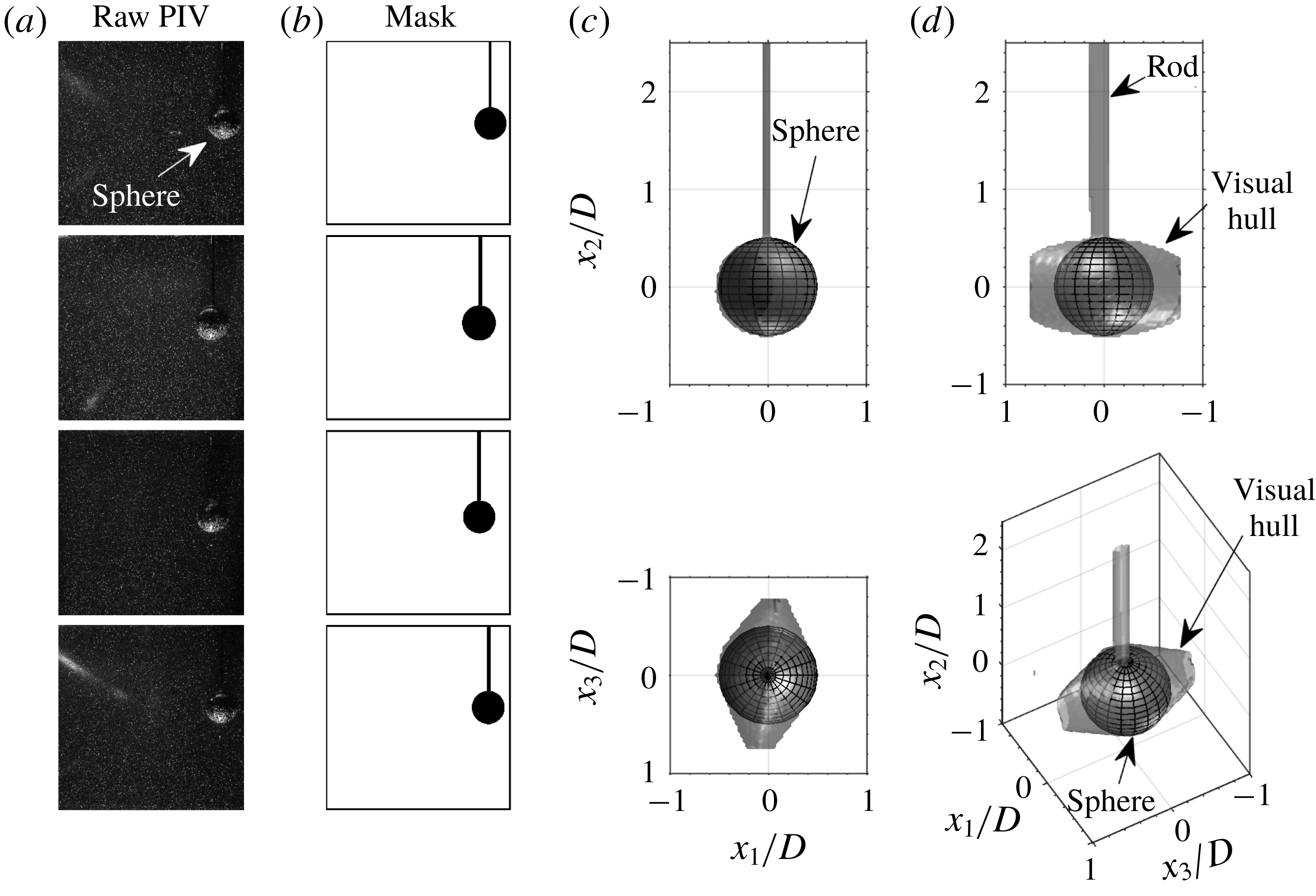
Due to the presence of the sphere in the VOI and the current camera configuration, some regions inside the VOI were not imaged. Prior to determining the vector fields, the sphere’s visual hull (including rod) was reconstructed based on 2-D masks of the sphere’s silhouette (figure 2, Adhikari & Longmire Reference Adhikari and Longmire2012; van Hout et al.
Reference van Hout, Eisma, Elsinga and Westerweel2018a
). Subsequently, the reconstructed 3-D particle volume was masked by the visual hull in order to remove ghost particles that appear within it and lead to spurious vectors. The visual hull resembles a dual cone (figure 2
c) as a result of the present camera layout (figure 1
b) and only its projection in the
 $x_{1}{-}x_{2}$
plane is circular.
Reconstruction of the visual hull. (a) Examples of raw PIV images for each camera and (b) the generated 2-D sphere masks; (c) projections of the reconstructed visual hull in the
 $x_{2}{-}x_{1}$
,
 $x_{3}{-}x_{1}$
,
 $x_{2}{-}x_{3}$
planes and a 3-D view of the visual hull. The sphere’s outer surface is illustrated by a grid in (c).

In order to determine the exact limits of the illuminated VOI in the
 $x_{3}$
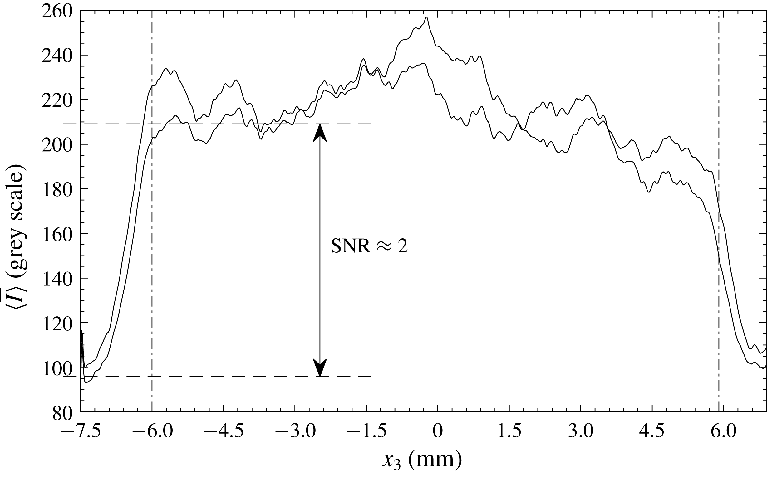
direction, the particle 3-D distribution was initially reconstructed over a larger depth than that of the VOI. The profile of the imaged particle intensity,
 $I$
, ensemble averaged over 20 reconstructed particle volumes and spatially averaged over
 $x_{1}$
and
 $x_{2}$
, resembled a top-hat profile (figure 3). Ghost particles at the outer limits of the reconstructed volume (figure 3) representing the noise level, displayed intensities of approximately 100 grey scales. Based on a signal-to-noise ratio,
 $\text{SNR}\approx 2$
(figure 3), the limits of the VOI in the
 $x_{3}$
direction (dash-dotted lines in figure 3) were defined by
 $-6.0~\text{mm}<x_{3}<6.0$
mm.
Ensemble and spatially averaged intensity profiles of the first and second exposure across the
 $x_{3}$
direction of the VOI.

Three-dimensional vector maps were obtained by multistep, 3-D cross-correlation while decreasing the interrogation volume in three steps from
 $64\times 64\times 64$
voxels (without overlap) to
 $40\times 40\times 40$
voxels with 75 % overlap, corresponding to a vector spacing of 0.2 mm. The dimension of the final interrogation volume was chosen to contain on average at least 5 particle pairs to ensure a high probability of valid vector detection (Adrian & Westerweel Reference Adrian and Westerweel2011). Between passes, universal outlier detection based on a median filter was performed (Westerweel & Scarano Reference Westerweel and Scarano2005) while at the end of each pass, a
 $3\times 3\times 3$
Gaussian smoothing filter was applied. The resulting vector maps were further spatially smoothed using a quadratic regression over 15 points in each direction (Elsinga et al.
Reference Elsinga, Adrian, van Oudheusden and Scarano2010) corresponding to 3 mm. Since at the present Reynolds number the sphere is characterized by large-scale structures (Sakamoto & Haniu Reference Sakamoto and Haniu1990; Johnson & Patel Reference Johnson and Patel1999) of the order of
 $D/2$
, the present choice of the regression scale is not expected to remove any relevant flow structures in the sphere wake. Spatial velocity gradients were based on the locally fitted quadratic regression (see Elsinga et al.
Reference Elsinga, Adrian, van Oudheusden and Scarano2010).
Instantaneous vortical structures in the flow were visualized using the
 $Q$
-criterion (Hunt, Wray & Moin Reference Hunt, Wray and Moin1988). The
 $Q$
-criterion defines vortices as regions where the magnitude of the rate-of-rotation exceeds that of the rate-of-strain:
 $$\begin{eqnarray}Q={\textstyle \frac{1}{2}}(\Vert \unicode[STIX]{x1D734}\Vert ^{2}-\Vert \unicode[STIX]{x1D64E}\Vert ^{2})>0,\end{eqnarray}$$
where
 $\unicode[STIX]{x1D61A}_{ij}=(\unicode[STIX]{x2202}U_{i}/\unicode[STIX]{x2202}x_{j}+\unicode[STIX]{x2202}U_{j}/\unicode[STIX]{x2202}x_{i})/2$
defines the rate-of-strain tensor, and
 $\unicode[STIX]{x1D6FA}_{ij}=(\unicode[STIX]{x2202}U_{i}/\unicode[STIX]{x2202}x_{j}-\unicode[STIX]{x2202}U_{j}/\unicode[STIX]{x2202}x_{i})/2$
defines the rate-of-rotation tensor. Note that
 $\Vert ..\Vert$
denotes the norm of a tensor, e.g.
 $\Vert \unicode[STIX]{x1D734}\Vert =[\text{tr}(\unicode[STIX]{x1D734}\unicode[STIX]{x1D734}^{\text{T}})]^{1/2}$
, where
 $\text{tr}$
denotes the trace of the tensor. Besides the
 $Q$
-criterion, the vorticity,
 $\unicode[STIX]{x1D74E}=\unicode[STIX]{x1D735}\times \boldsymbol{u}$
, was used to quantify the rotation direction of the vortices. The data quality and in particular the spatial velocity gradients, were assessed by evaluating the residual of the continuity equation for an incompressible fluid,
 $\unicode[STIX]{x2202}U_{i}/\unicode[STIX]{x2202}x_{i}=0$
. The joint probability distribution of
 $\unicode[STIX]{x2202}U_{3}/\unicode[STIX]{x2202}x_{3}$
and
 $-(\unicode[STIX]{x2202}U_{1}/\unicode[STIX]{x2202}x_{1}+\unicode[STIX]{x2202}U_{2}/\unicode[STIX]{x2202}x_{2})$
was distributed as an elongated ellipse along the diagonal that would represent a perfectly satisfied continuity equation (see also van Hout et al.
Reference van Hout, Eisma, Elsinga and Westerweel2018a
). The correlation coefficient,
 $R^{2}$
, between the two quantities was 0.87, i.e. comparable to
 $R^{2}$
values obtained by Zhang, Tao & Katz (Reference Zhang, Tao and Katz1997) and Casey, Sakakibara & Thoroddsen (Reference Casey, Sakakibara and Thoroddsen2013).
4 Results
4.1 Instantaneous 3-D vortex structure
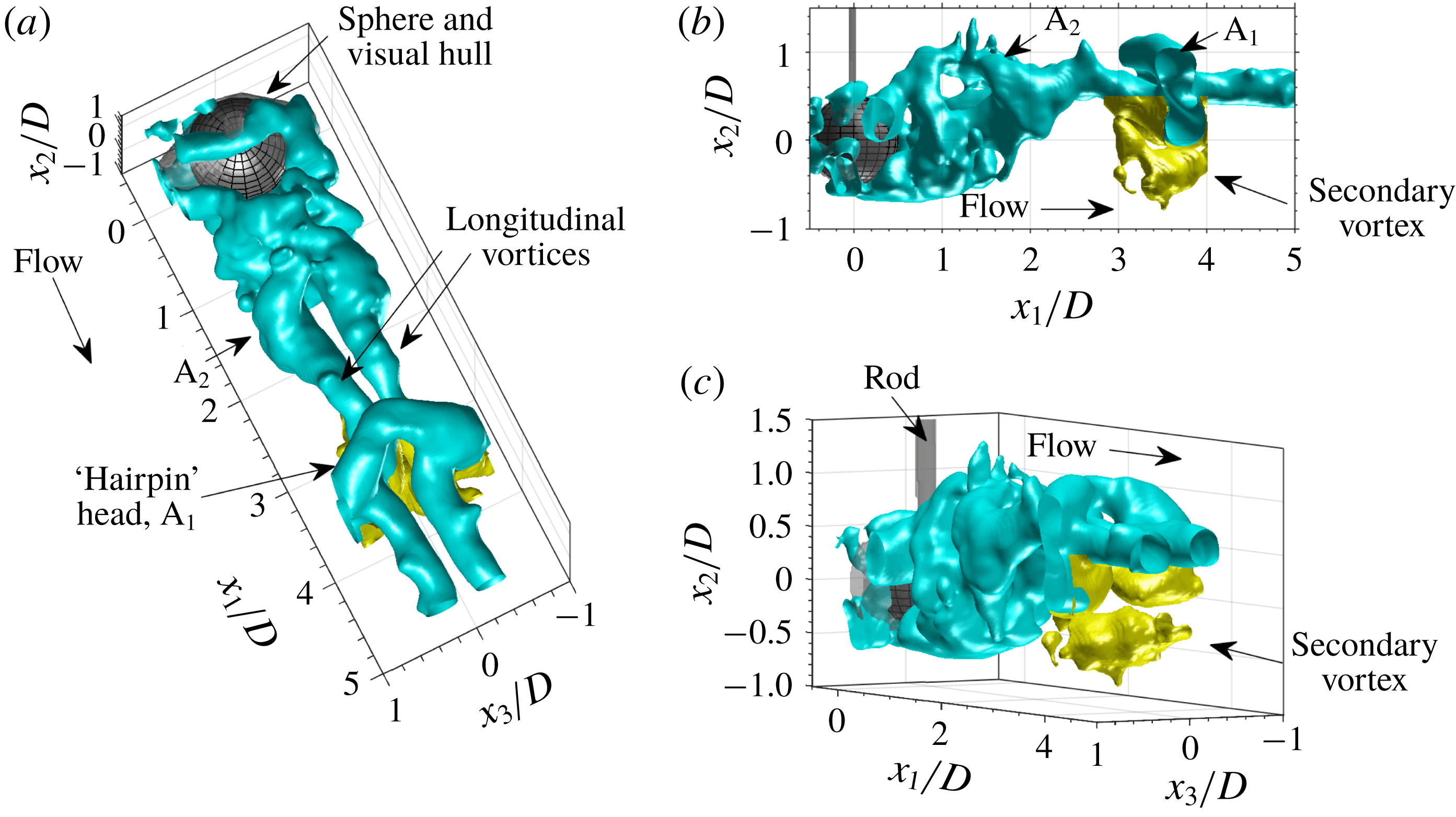
Example snapshot of the instantaneous 3-D vortex structure in the wake of the sphere visualized by the
 $Q$
-criterion (3.1). Cyan and yellow iso-surfaces depict the shed primary vortices and the secondary vortex, respectively. This snapshot corresponds to
 $tU/D=2.625$
(§§ 4.3 and 4.4, figure 15).

A representative snapshot of the instantaneous 3-D wake structure visualized by the
 $Q$
-criterion (3.1) is displayed in figure 4. The shed primary vortices (depicted in cyan) clearly resemble those observed in dye visualizations (e.g. Sakamoto & Haniu Reference Sakamoto and Haniu1990; Johnson & Patel Reference Johnson and Patel1999; Leweke et al.
Reference Leweke, Provansal, Ormieres and Lebescond1999). Two parallel, longitudinal vortices extend from the near-wake region of the sphere in the streamwise direction (figure 4
a) and are connected to each other by an upward directed arch completing a ‘hairpin’ head. Similar to dye visualizations, a series of entangled hairpin vortices can be observed in figure 4. The instantaneous snapshot shows one hairpin head (
 $\text{A}_{1}$
) located between
 $3<x_{1}/D<4$
while a second one (
 $\text{A}_{2}$
) positioned at
 $x_{1}/D\approx 1.5$
, is close to being shed. In the latter case, there is still a connection at the top but the upward pointing parts of the arch have already detached from the near wake (figure 4
b). Note that the hairpins were always shed at the same orientation with their ‘heads’ pointed upwards (figure 4
a). This constant orientation of the shed hairpins has been observed in most experimental and numerical studies at similar Reynolds numbers and once the first hairpin is created, the following are generated by a repeating process of cross-wake movement of the near-wake structure in a manner that maintains their orientation (see Johnson & Patel Reference Johnson and Patel1999). In the present measurements, the initial hairpin orientation is likely to be induced by the rod’s attachment location on the top of the sphere.
Besides the shed ‘hairpin’ vortices, secondary vortices (depicted in yellow in figure 4) were detected in the instantaneous snapshots. The latter have never been observed in dye visualization studies because the dye only marks streaklines, and have only been reported in the DNS results by Johnson & Patel (Reference Johnson and Patel1999) where they were coined ‘induced’ vortices, and in the planar PIV experiments by Brücker (Reference Brücker2001). The secondary vortices were weaker than the shed ‘hairpin’ vortices at this stage of their development and were always positioned below the ‘hairpin’ heads of the shed vortices. Distinct secondary vortex legs do not appear in the
 $Q$
-criterion visualization. Their generation mechanism will be further discussed in § 4.4.
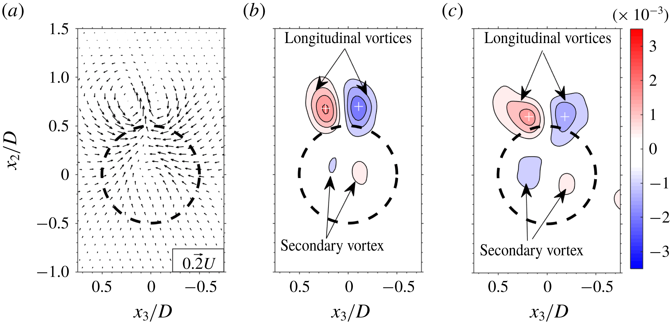
Transverse planes of (a) the instantaneous 2-D vector field (for clarity depicted at
 $1/12$
the actual spatial resolution) at
 $x_{1}/D=2.5$
, and the associated out-of-plane vorticity distribution,
 $\unicode[STIX]{x1D714}_{1}D/U$
, at
 $x_{1}/D$
 $=$
(b) 2.5, (c) 3.0. Data correspond to the instantaneous snapshot depicted in figure 4. Level list in (b) and (c):
 $\pm [0.5:0.5:3.5]\times 10^{-3}$
, denoting [lower limit : step size : upper limit]. Dashed circle depicts sphere perimeter.

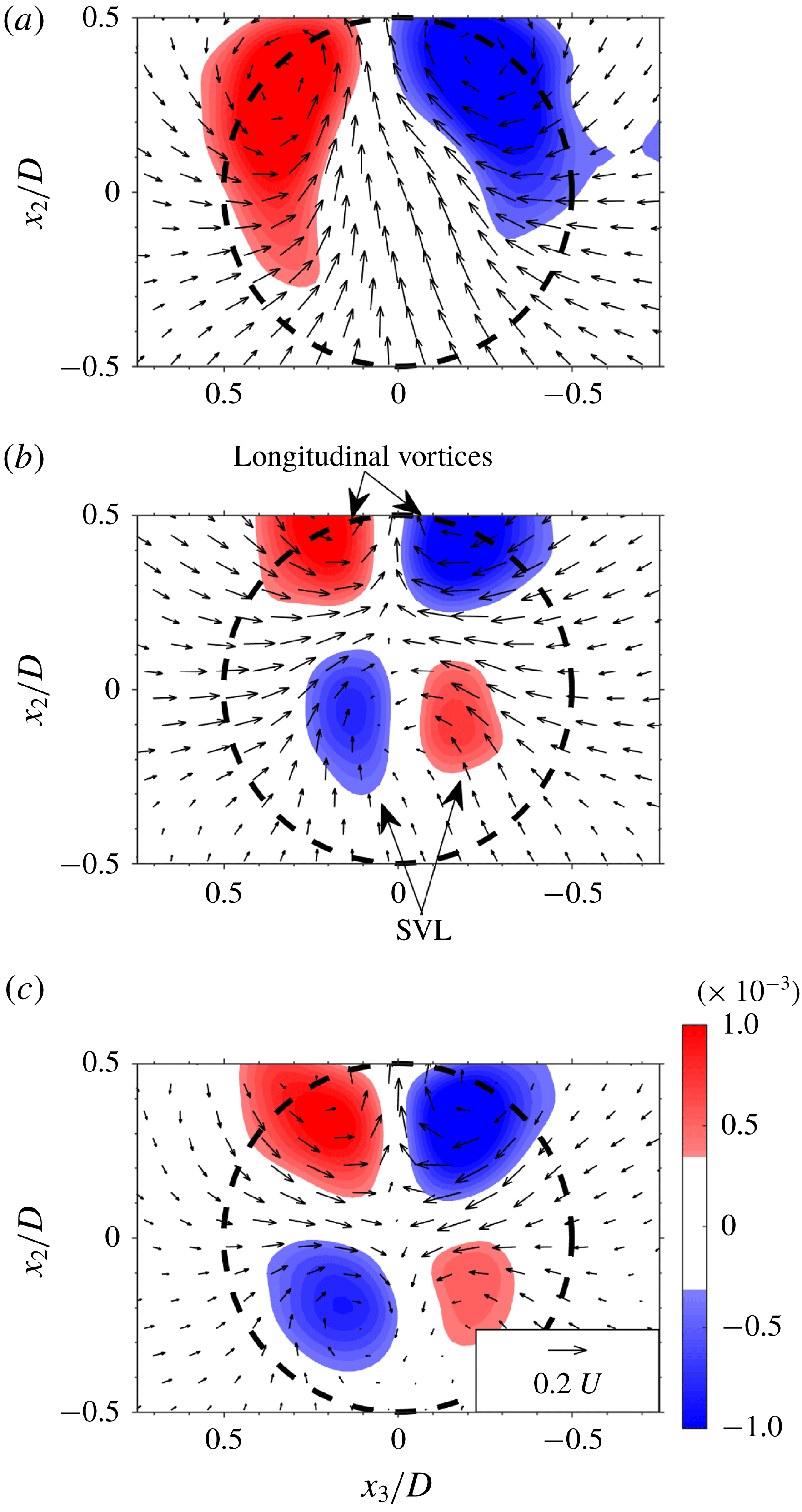
To get a better idea of the instantaneous flow field that is generated by the vortices depicted in figure 4, the instantaneous 2-D vector field and out-of-plane vorticity component are plotted in transverse planes at
 $x_{1}/D=2.5$
and 3.0 in figure 5 and in a vertical equatorial plane (
 $x_{3}/D=0$
) in figure 6. The instantaneous 2-D vector field and vorticity distribution displayed in figure 5 clearly show two counter-rotating vortices that are the cross-sections of the longitudinal vortices that connect between the ‘hairpin’ heads
 $\text{A}_{1}$
and
 $\text{A}_{2}$
in figure 4. As expected, these longitudinal vortices expel fluid upwards (in the positive
 $x_{2}$
-direction) in between them, and are located just above the sphere (its outline indicated by a dash black circle) as a result of self-induction. The vortex centres associated with the longitudinal vortices are located in the range
 $x_{2}/D\approx 0.6$
to 0.7 (indicated by ‘
 $+$
’ in figure 5
b,c). The streamwise vorticity distribution at
 $x_{1}/D=2.5$
and 3.0 (figure 5
b,c), is characterized by opposite sign patches of
 $\unicode[STIX]{x1D714}_{1}$
associated with the longitudinal vortices while smaller patches of counter-rotating vorticity associated with the secondary vortex appear inside the perimeter of the sphere. The latter’s rotation direction is opposite of those of the longitudinal vortices located just above them.
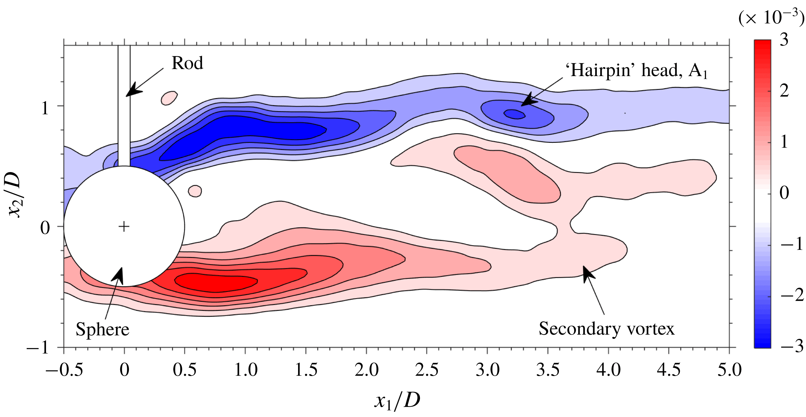
Vertical equatorial plane (
 $x_{3}/D=0$
) depicting the out-of-plane vorticity distribution,
 $\unicode[STIX]{x1D714}_{3}D/U$
. Data correspond to the instantaneous snapshot shown in figure 4.

The distribution of
 $\unicode[STIX]{x1D714}_{3}D/U$
in the vertical (
 $x_{1}{-}x_{2}$
) equatorial plane (figure 6) further illustrates the generated vorticity field. Strong shear layers extend from the periphery of the sphere in the streamwise direction. Both the ‘head’ of the hairpin,
 $\text{A}_{1}$
, as well as that of the secondary vortex are represented by patches of positive and negative
 $\unicode[STIX]{x1D714}_{3}$
, respectively, in the range
 $3.0<x_{1}/D<4.0$
.
4.2 Mean velocities
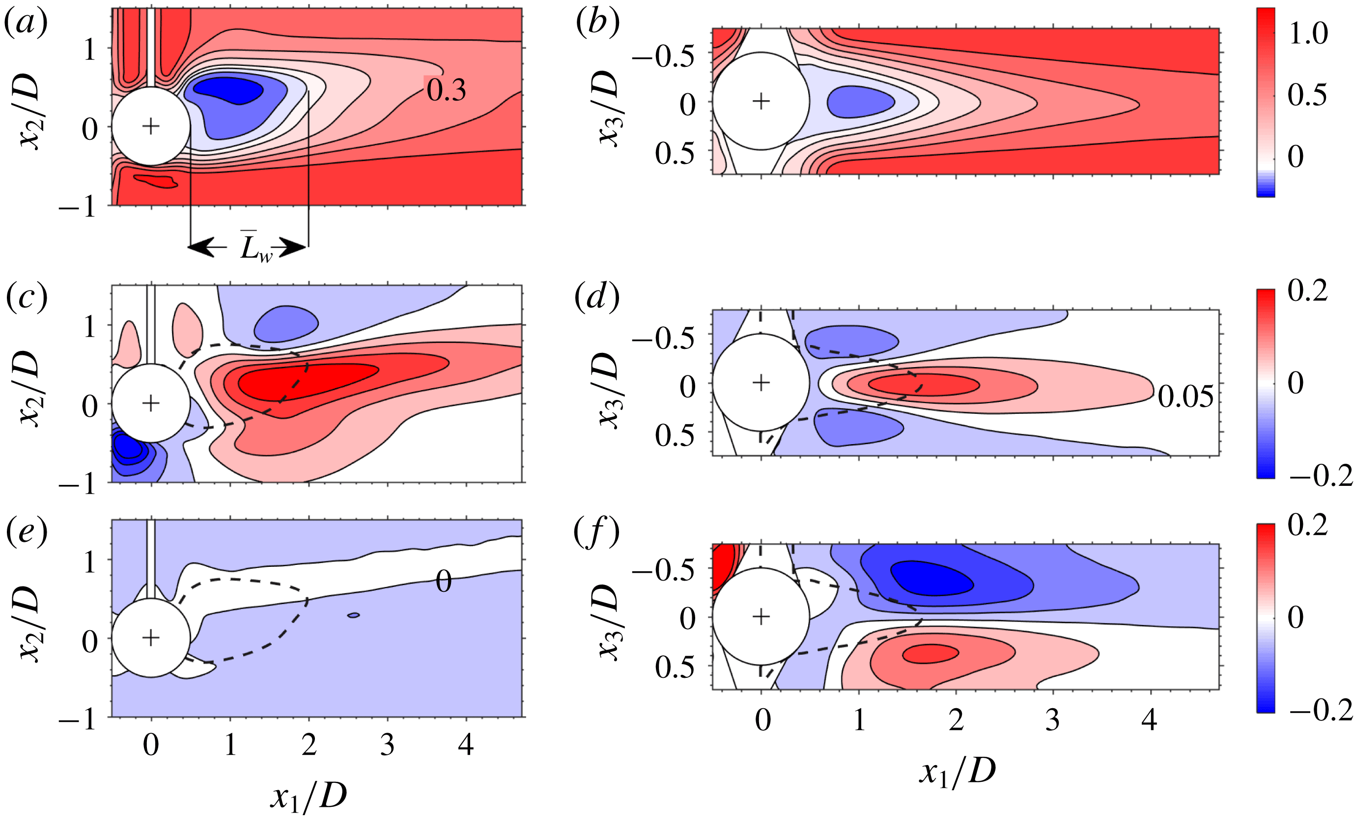
Normalized, ensemble averaged velocity components in equatorial planes. (a,c,e) Vertical (
 $x_{1}{-}x_{2}$
) planes, (b,d,f) horizontal (
 $x_{1}{-}x_{3}$
) planes; (a,b)
 $\overline{U}_{1}/U$
, (c,d)
 $\overline{U}_{2}/U$
, (e,f)
 $\overline{U}_{3}/U$
. The dashed black curve in (c–f) depicts the border of the ensemble averaged recirculating wake extracted from (a) and (b). Level lists: (a,b) [
 $-0.3:0.1:0~0.1:0.2:1.2$
], (c–f) [
 $-0.2:0.05:0.2$
]; example levels are depicted in (a,d,e). The silhouettes of the sphere, rod and visual hull are depicted in white and the sphere’s centroid by ‘
 $+$
’.

Contour plots of the normalized, time averaged velocity components,
 $\overline{U}_{i}/U$
(
 $i=1$
–3), are depicted in horizontal (
 $x_{1}{-}x_{3}$
) and vertical (
 $x_{1}{-}x_{2}$
) equatorial planes in figure 7. The streamwise component (figure 7
a,b) clearly shows a recirculating wake for which
 $\overline{U}_{1}/U<0$
(blue in figure 7
a,b). The mean recirculating wake length,
 $\overline{L}_{w}$
, is defined here as the distance from the downstream end of the sphere to the downstream position where
 $\overline{U}_{1}$
changes sign (figure 7
a). The border of the recirculating wake defined by the positions where
 $\overline{U}_{1}$
changes sign (
 $\overline{U}_{1}/U=0$
in figure 7
a,b), is depicted as a dashed black curve in figure 7(c–f). As observed, distributions of all three velocity components in the
 $x_{1}{-}x_{3}$
plane (figure 7
b,d,f) are symmetric with respect to
 $x_{3}/D=0$
. In contrast, the mean velocity distributions in the
 $x_{1}{-}x_{2}$
plane (figure 7
a,c,e) show that axisymmetry is lost at this Reynolds number (see also Sakamoto & Haniu Reference Sakamoto and Haniu1990; Johnson & Patel Reference Johnson and Patel1999; Ploumhans et al.
Reference Ploumhans, Winckelmans, Salmon, Leonard and Warren2002). The time averaged recirculating wake is directed upwards in the positive
 $x_{2}$
direction as a result of the induced motion of the shed primary vortices discussed in the previous section (figures 4 to 6). The mean induced velocity field in the
 $x_{2}$
-direction as a result of the rotational motion of the longitudinal vortices can be clearly observed in figure 7(c,d).
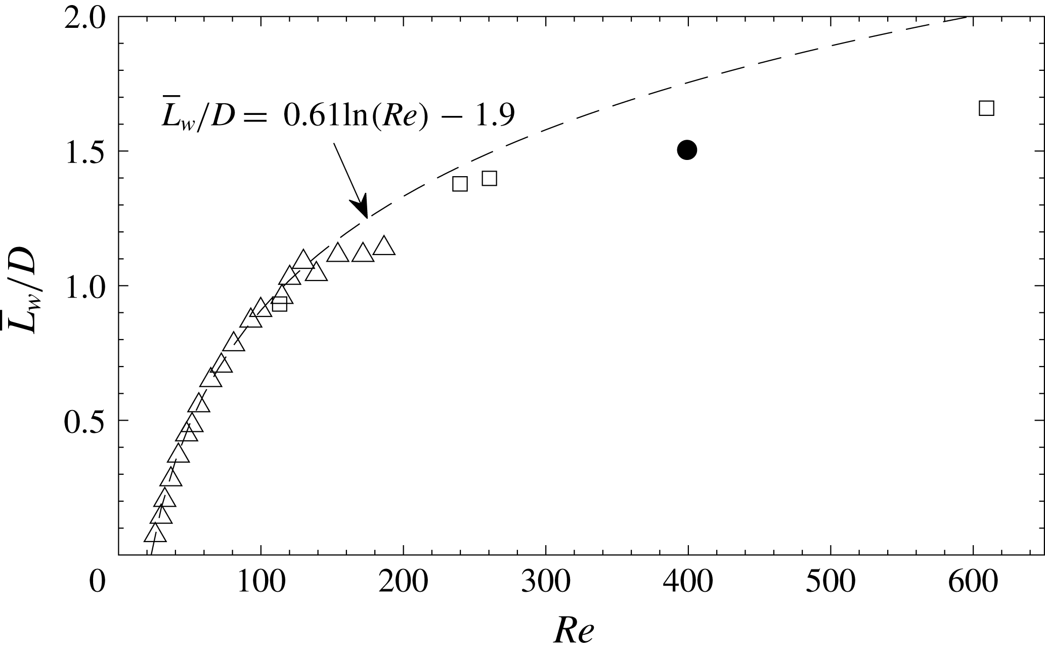
A comparison of the present mean, recirculating wake length to available measurements by Taneda (Reference Taneda1956) and DNS results by Bagchi & Balachandar (Reference Bagchi and Balachandar2004) (figure 8) shows that the present
 $\overline{L}_{w}$
falls well within the range investigated by Bagchi & Balachandar (Reference Bagchi and Balachandar2004) and follows the asymptotic behaviour with increasing
 $Re$
indicated by the results of Taneda (Reference Taneda1956) and Bagchi & Balachandar (Reference Bagchi and Balachandar2004). The rod does not seem to adversely affect the mean recirculating wake length. Furthermore up to
 $Re\approx 200$
,
 $\overline{L}_{w}/D$
is fitted well by the least-square exponential fit (based on the first 17 points of Taneda (Reference Taneda1956)) depicted in figure 8. Beyond this
 $Re$
,
 $\overline{L}_{w}/D$
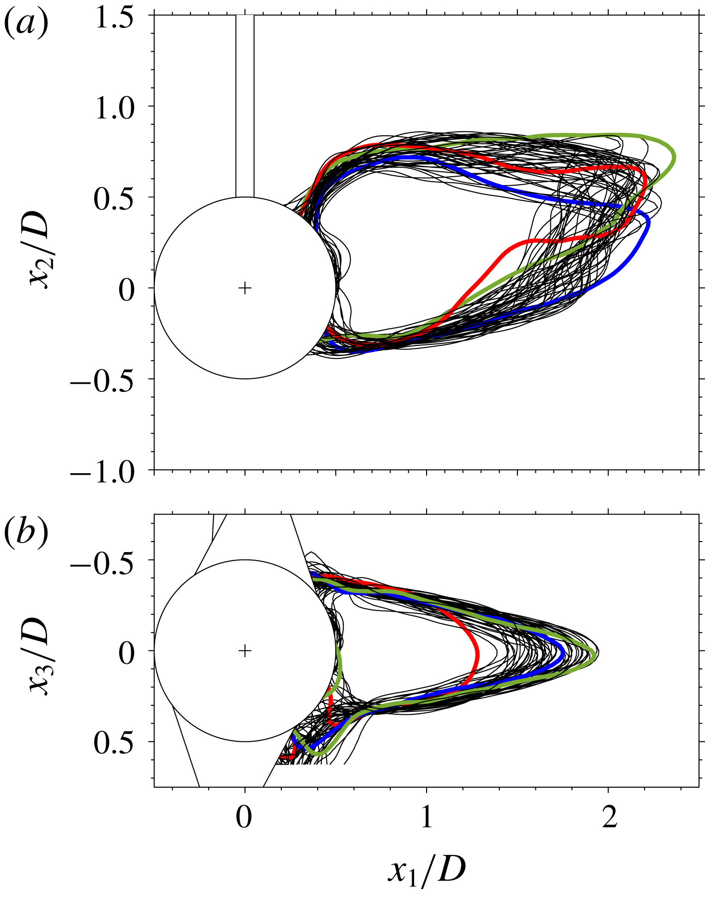
is overpredicted by the fit. To get an idea of the degree of wake unsteadiness as a result of vortex shedding, examples of superposed instantaneous borders of the recirculating wake defined as the locations where
 $U_{1}$
changes sign, are plotted in figure 9 in
 $x_{1}{-}x_{2}$
and
 $x_{1}{-}x_{3}$
planes. The instantaneous recirculating wake changes quite significantly both in shape as well as in extent at this
 $Re$
, similar to DNS results presented by Bagchi & Balachandar (Reference Bagchi and Balachandar2004).
The ensemble averaged, normalized recirculating wake length as a function of
 $Re$
. ▵ Taneda (Reference Taneda1956), ▫ Bagchi & Balachandar (Reference Bagchi and Balachandar2004), ● present result, (dashed curve) least-square exponential fit to first 17 points of Taneda (Reference Taneda1956).

Examples of superposed instantaneous recirculating wake borders (
 $U_{1}/U=0$
) in equatorial (a)
 $x_{1}{-}x_{2}$
and (b)
 $x_{1}{-}x_{3}$
planes. For clarity, some instantaneous borders are coloured. The silhouettes of the sphere, rod and visual hull are depicted in white and the sphere’s centroid by ‘
 $+$
’.

4.3 Vortex shedding sequence
The present tomo-PIV measurements were not temporally resolved. However, at this
 $Re$
, periodic vortex shedding is obtained (Sakamoto & Haniu Reference Sakamoto and Haniu1990), and in order to reconstruct an ensemble averaged vortex shedding sequence, the following data processing procedure based on combining the tomo-PIV with the planar TR-PIV was implemented. First, instantaneous tomo-PIV snapshots were binned based on the planar signatures of the directional swirling strength (e.g. Krakovich et al.
Reference Krakovich, Eshbal and Van Hout2013) in vertical equatorial planes. As discussed in § 4.1, vortex shedding is characterized by shed sequences of strong, longitudinal vortices interconnected by transverse arches (shed ‘hairpin’ heads) as well as weaker secondary vortices in the initial stages of their development (figure 4). Vertical equatorial planes of directional swirling strength isolate the vortex cores associated with the shed ‘hairpin’ heads (see van Hout et al.
Reference van Hout, Krakovich and Gottlieb2010) and using ‘blob’ analysis (Matlab toolbox) their centroid positions were determined (van Hout, Rinsky & Grobman Reference van Hout, Rinsky and Grobman2018b
). Based on the
 $x_{1}$
coordinate of the centroid positions, the instantaneous tomo-PIV snapshots were binned (bin size
 $\unicode[STIX]{x0394}x_{1}=0.5D$
) and subsequently ensemble averaged for each bin. The number of snapshots in each bin exceeded 80. The associated temporal information was determined from the TR-PIV by cross-correlating horizontal equatorial planes of
 $\unicode[STIX]{x1D714}_{2}$
with those of the ‘binned’ ensemble averaged tomo-PIV sequence. In addition to this, the temporal vortex shedding sequence was also reconstructed by directly cross-correlating the out-of-plane vorticity component (
 $\unicode[STIX]{x1D714}_{2}$
) obtained by the TR-PIV with overlapping instantaneous equatorial tomo-PIV planes and subsequent data binning. Similar end results were obtained by both procedures, but the first procedure was more robust and therefore its results are presented in the following discussion.
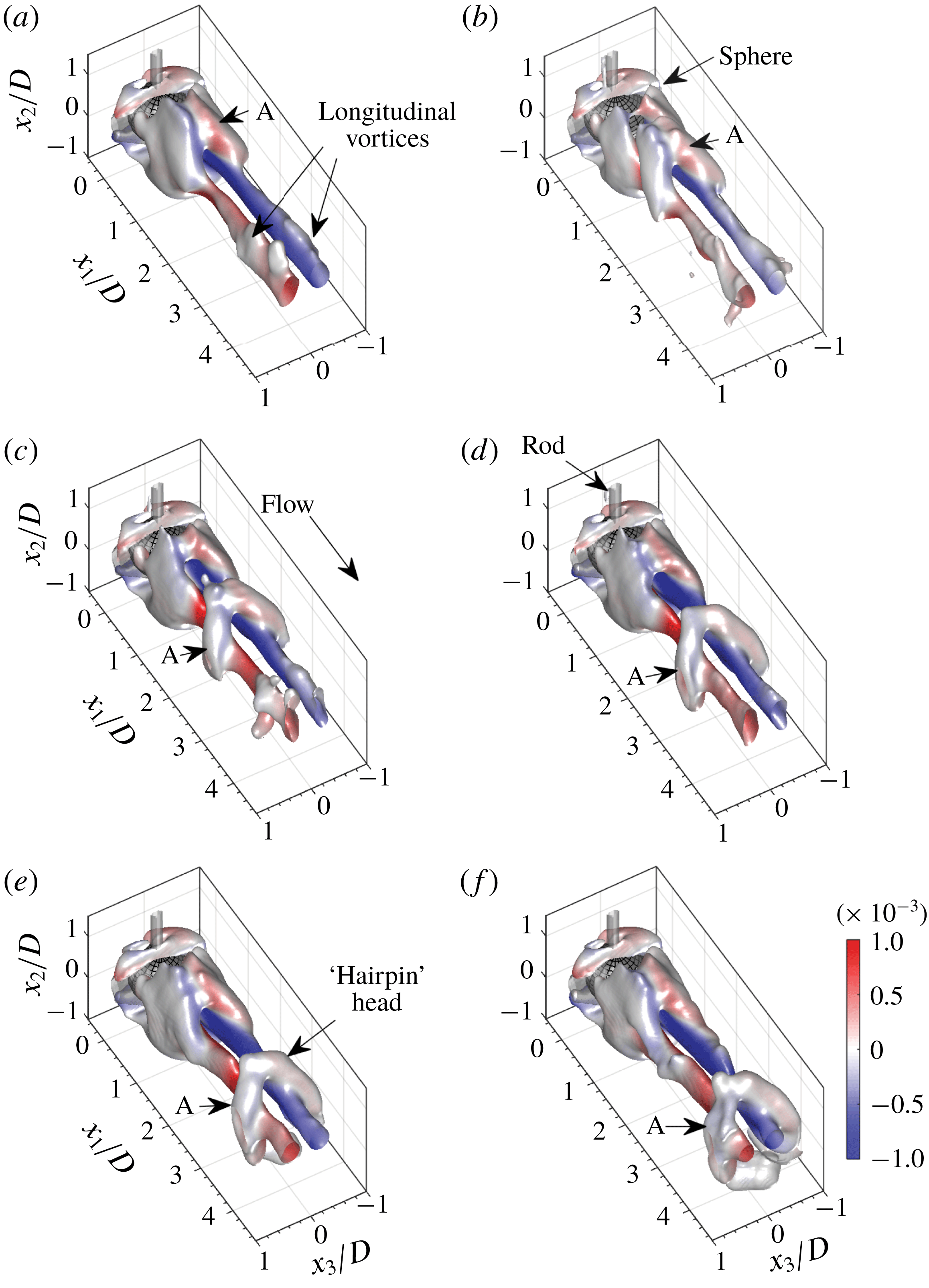
Top view of 3-D surface plots of the ensemble averaged, vortex shedding cycle in the wake of the sphere;
 $Q$
-criterion overlaid by
 $\overline{\unicode[STIX]{x1D714}}_{1}D/U$
.
 $tU/D$
 $=$
(a) 0, (b) 0.75, (c) 1.5, (d) 2.25, (e) 3.0 and (f) 3.75.

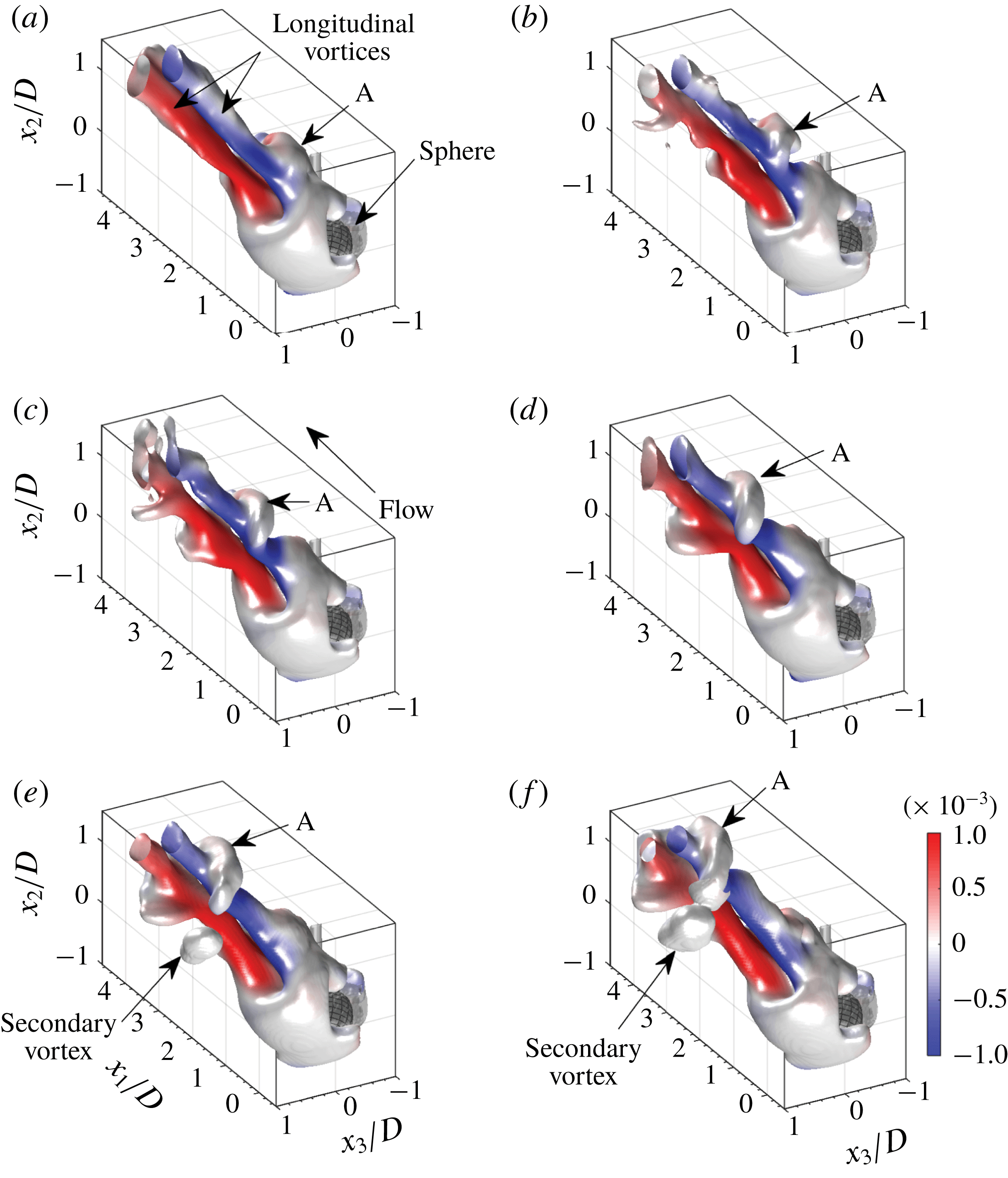
Bottom view of 3-D surface plots of the ensemble averaged, vortex shedding cycle in the wake of the sphere;
 $Q$
-criterion overlaid by
 $\overline{\unicode[STIX]{x1D714}}_{1}D/U$
.
 $tU/D$
 $=$
(a) 0, (b) 0.75, (c) 1.5, (d) 2.25, (e) 3.0 and (f) 3.75.

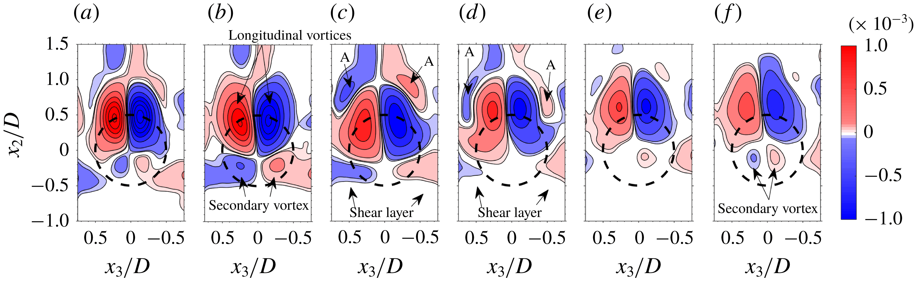
Three-dimensional, top and bottom views (looking from the downstream to the upstream direction) of the ensemble averaged vortex shedding sequence, overlaid by the normalized, ensemble averaged streamwise component of the vorticity,
 $\overline{\unicode[STIX]{x1D714}}_{1}D/U$
, are depicted in figures 10 and 11, respectively, at twice the available temporal resolution. As can be observed, the 3-D vortex structure in the instantaneous snapshot (figure 4) has been preserved. The two longitudinal vortices extending from the near wake are counter-rotating (figures 10 and 11) and expel fluid upwards (see also figures 4 and 5). In figure 10(a) (
 $tU/D=0$
), a ‘hairpin’ head (A) barely attached to the sphere’s recirculating wake is seen to have developed. It detaches in figure 10(b) (
 $tU/D=0.75$
) and moves downstream of the sphere with increasing
 $tU/D$
. It is seen that the ‘hairpin’ head ‘embraces’ the longitudinal vortices that do not show any discontinuity before and after it. The bottom view shown in figure 11, shows that the secondary vortex appears only after the shed ‘hairpin’ head, A, is already fully developed at
 $tU/D=3.0$
(figures 10
e and 11
e). Note that the first sign of the secondary vortex was detected at
 $tU/D=2.625$
(not shown). The streamwise inception location of the secondary vortex lies in the range
 $3.0<x_{1}/D<4.0$
in good agreement with the DNS of Johnson & Patel (Reference Johnson and Patel1999).
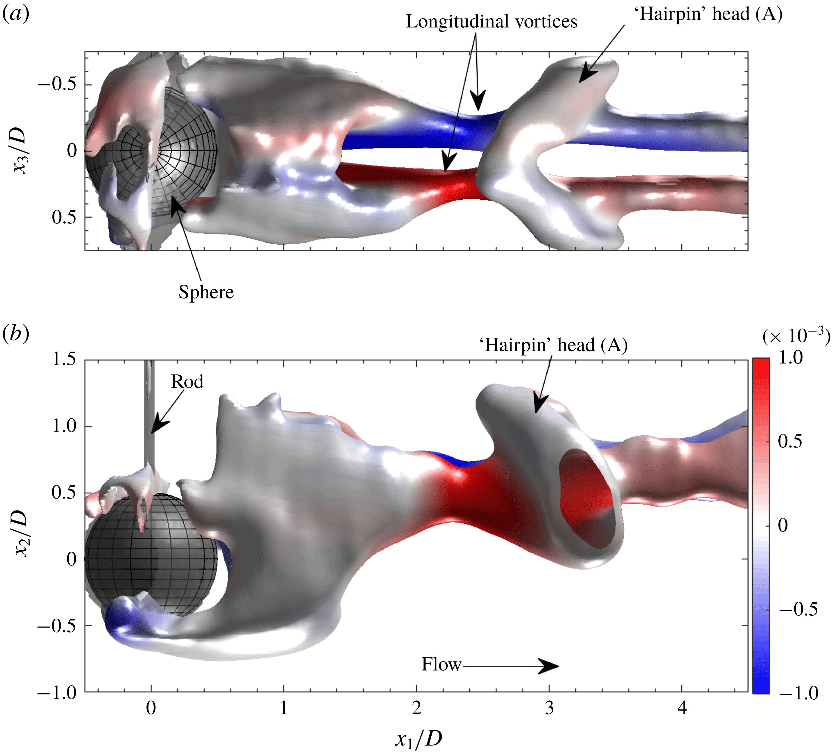
Projections of 3-D surface plots of the
 $Q$
-criterion overlaid by
 $\overline{\unicode[STIX]{x1D714}}_{1}D/U$
at
 $tU/D=2.25$
. (a) Top view, (b) side view.

Top and side views of the 3-D surface plot at
 $tU/D=2.25$
, just before the secondary vortex head appears, are shown in figure 12. Note that the ‘hairpin’ head (A) is tilted towards the sphere at an angle of about
 $50^{\circ }$
with the horizontal as a result of the rod. To get a better idea of the associated vorticity distribution, slices of
 $\overline{\unicode[STIX]{x1D714}}_{1}D/U$
contours in
 $x_{2}{-}x_{3}$
planes (figure 13) and
 $x_{1}{-}x_{3}$
planes (figure 14) at several
 $x_{1}/D$
and
 $x_{2}/D$
locations, respectively, are investigated for
 $tU/D=2.25$
(figures 10
d, 11
d and 12). As expected, the
 $x_{2}{-}x_{3}$
planes (figure 13) indicate strong regions of opposite sign
 $\overline{\unicode[STIX]{x1D714}}_{1}$
located at the centroid positions of the longitudinal vortices extending from the near wake (depicted in figure 12). At
 $x_{1}/D=2$
and 2.5 (figure 13
a,b) two small opposite sign, much weaker vorticity regions develop just below those associated with the longitudinal vortices (figure 13
b). These weak regions disappear at
 $x_{1}/D=3.0$
and 3.5 (figure 13
c,d) but reappear at
 $x_{1}/D=4.0$
and 4.5 (figure 13
e,f). They represent the planar vorticity signatures of parts of the secondary vortices observed in the instantaneous snapshots (figures 4 and 11
e,f) and have previously been observed in the DNS results by Johnson & Patel (Reference Johnson and Patel1999) and in the planar PIV measurements by Brücker (Reference Brücker2001). Their appearance at
 $x_{1}/D\approx 2.5$
and 4.5 shows that they consistently exist in conjunction with the ‘hairpin’ heads generated as a result of vortex shedding. The secondary vortices are weaker than the shed primary vortices and the present measurements only capture their initial development. In addition, vorticity patches associated with the ‘hairpin’ head (A) (see also figures 10 to 12) can be seen in the cross-sections at
 $x_{1}/D=3.0$
and 3.5, shown in figures 13(c) and 13(d), respectively.
The description above is further strengthened by vorticity contours of
 $\overline{\unicode[STIX]{x1D714}}_{1}D/U$
in
 $x_{1}{-}x_{3}$
planes at several
 $x_{2}$
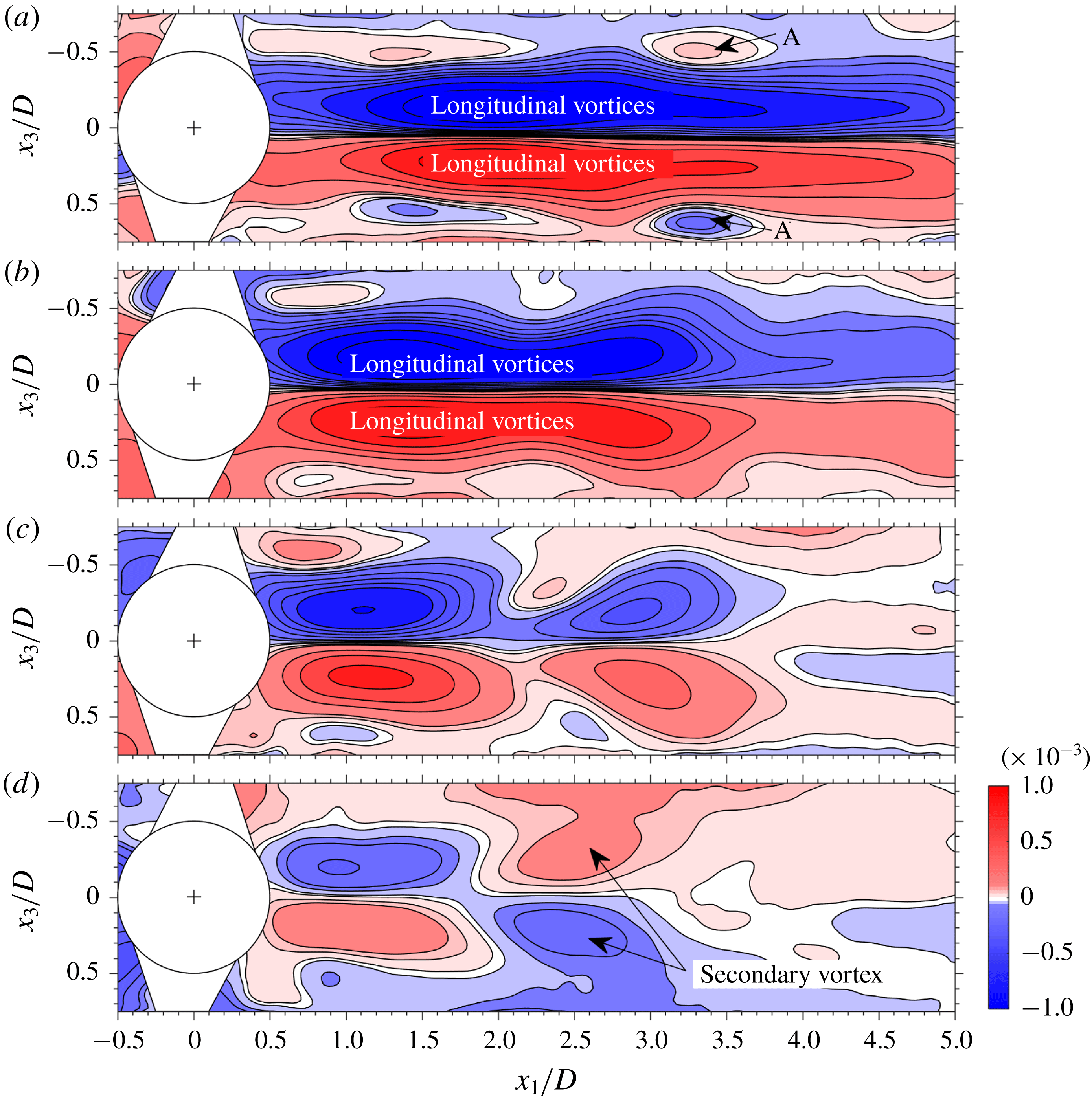
positions (depicted in figure 14). At
 $x_{2}/D=0.5$
and 0.25 (figure 14
a,b), strong planar vorticity signatures of the longitudinal vortices are seen. Two opposite sign vorticity patches associated with the hairpin head (A) are clearly observed in figure 14(a). The first indication of streamwise vorticity associated with the secondary vortices is seen at
 $x_{2}/D=0$
(figure 14
c) where at
 $x_{1}/D\approx 2.5$
small patches of opposite sign vorticity appear. These grow in size and strength at
 $x_{1}/D=-0.25$
(figure 14
d). The formation of the secondary vortices will be further discussed in § 4.4.
Contour slices in the
 $x_{2}{-}x_{3}$
plane of the ensemble averaged streamwise vorticity component,
 $\overline{\unicode[STIX]{x1D714}}_{1}D/U$
, at different downstream positions.
 $x_{1}/D$
 $=$
(a) 2.0, (b) 2.5, (c) 3.0, (d) 3.5, (e) 4.0 and (f) 4.5;
 $tU/D=2.25$
(see figures 10
d, 11
d and 12). Level list:
 $\pm [0.03~0.05~0.15:0.3:2.85]\times 10^{-3}$
.

Contour slices in the
 $x_{1}{-}x_{3}$
plane of the ensemble averaged streamwise vorticity component,
 $\overline{\unicode[STIX]{x1D714}}_{1}D/U$
, at different vertical positions,
 $x_{2}/D$
 $=$
(a) 0.5, (b) 0.25, (c) 0 and (d)
 $-0.25$
;
 $tU/D=2.25$
(see figures 10
d and 11
d). Level list:
 $\pm [0.01~0.06~0.1:0.1:0.5~0.8:0.4:2]\times 10^{-3}$
.

4.4 Vortex shedding mechanism and generation of secondary vortices
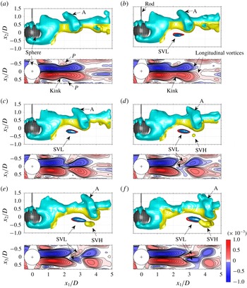
The present data allow us to investigate in detail the mechanism of vortex shedding and generation of the secondary vortices. The temporal vortex shedding sequence and the emergence of the secondary vortices are illustrated for the ensemble averaged data set in figure 15 by a combination of 3-D iso-surfaces of the
 $Q$
-criterion, of
 $\overline{\unicode[STIX]{x1D714}}_{1}D/U$
and associated contour plots of the streamwise vorticity component in equatorial
 $x_{1}{-}x_{3}$
planes. Prior to the emergence of the secondary vortex head (SVH) that first appears at
 $tU/D=2.625$
, in the range
 $3.0<x_{1}/D<3.5$
(figure 15
d), the secondary vortex legs (SVL) become visible in the iso-surfaces of the streamwise vorticity component (depicted in blue and red in figure 15) at
 $tU/D=1.875$
(figure 15
b). The secondary vortex head is located below the shed ‘hairpin’ head (A) and both are advected downstream while the secondary vortex gains strength (figure 15
d–f), resembling the DNS results by Johnson & Patel (Reference Johnson and Patel1999).
The equatorial (
 $x_{1}{-}x_{3}$
) planes of
 $\overline{\unicode[STIX]{x1D714}}_{1}D/U$
depicted below each iso-surface plot in figure 15 show that streamwise vorticity patches associated with the counter-rotating longitudinal vortices are strong and extend from the near wake of the sphere up to
 $x_{1}/D\approx 3.0$
(figure 15
a,b). A ‘kink’ appears at
 $x_{1}/D\approx 2.0$
(figure 15
a,b), as a result of a combination of vortex stretching and the drawing of fluid from below the sphere as will be discussed in the following. Furthermore, at this position at each side of the extended streamwise vorticity patches (associated with the longitudinal vortices), a small shear layer patch (
 $P$
) of opposite sign vorticity exists that is associated with the generation of the secondary vortex (see also figure 13). As the ‘hairpin’ head moves downstream (figure 15
d–f), the secondary vortex legs appear in the equatorial planes. As can be observed, they are positioned close to the centreline with their legs pointed inwards in the upstream direction. In none of the shedding stages, a connection between the upstream ‘hairpin’ head and the downstream secondary vortex legs could be detected. Note that the secondary vortex legs (SVL) first appear as iso-surfaces of
 $\overline{\unicode[STIX]{x1D714}}_{1}D/U$
at
 $tU/D=1.875$
(figure 15
b). At this downstream location, their rotation rate is not sufficiently strong compared to the strain rate and they do not appear in the
 $Q$
-criterion iso-surfaces.
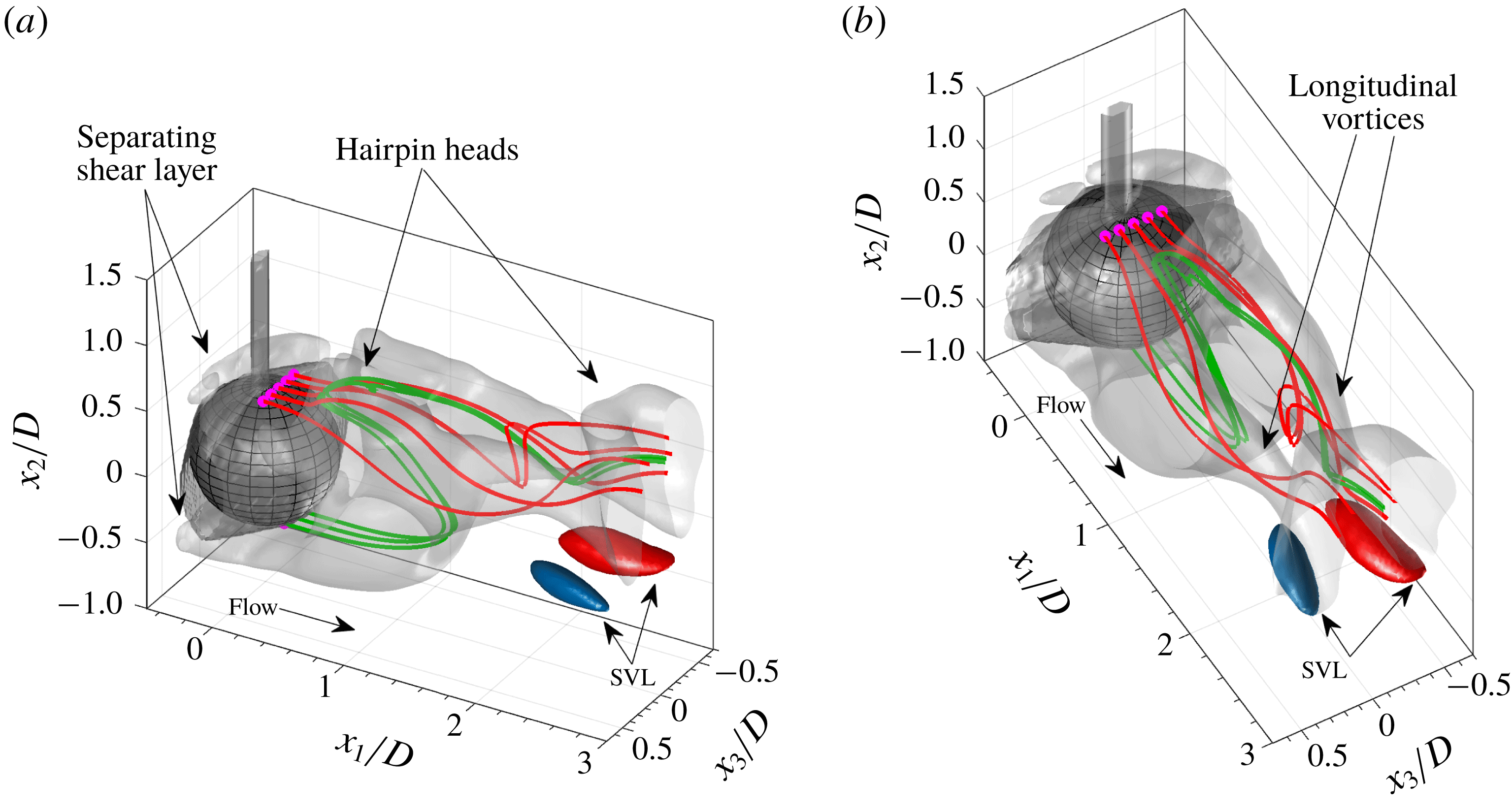
As observed in figures 10 and 11, the ‘hairpin’ heads (A) embrace the longitudinal vortices and do not form a logical extension to them. Magarvey & MacLatchy (Reference Magarvey and MacLatchy1965) and Taneda (Reference Taneda1978) described how transverse vorticity components resulting from the involution of the separating, annular shear layer are transformed into streamwise vorticity creating a pair of counter-rotating longitudinal vortices extending downstream. The pair of longitudinal vortices (figures 10 and 11) remains in place at all stages of the vortex shedding and are ‘fed’ by transforming transverse vorticity into streamwise vorticity by the lower bight in the near wake (see also Magarvey & MacLatchy Reference Magarvey and MacLatchy1965; Taneda Reference Taneda1978), while the upper bight is ‘rebuilt’ by a combination of shear layer involution and fluid drawn from below the sphere through the action of the pair of longitudinal vortices (Johnson & Patel Reference Johnson and Patel1999). As the upper bight moves away from the sphere and gains strength, a ‘hairpin’ head will be shed. This mechanism is illustrated in figure 16 that presents a close-up of the vortical structure in the near wake of the sphere just prior to shedding of the ‘hairpin’ head closest to the sphere, together with streamlines initiated just below the sphere (in green) and at the top of the sphere (in red). The separating shear layer sheet, a pair of longitudinal vortices as well as the ‘hairpin’ heads can be clearly discerned (see figure 16). Note that due to the visual hull and the rod, the separating shear layer is not fully resolved and only the top and bottom part are resolved (see also figure 12). The pair of longitudinal vortices draw fluid from below the sphere (
 $x_{2}/D<0$
) and streamlines (in green) started from below first enter the wake, subsequently are deflected by the ‘hairpin’ head and finally ‘ejected’ downstream into the counter-rotating longitudinal vortices, similar as described by Johnson & Patel (Reference Johnson and Patel1999). At this time instant, streamlines that are initiated from the top of the sphere (in red, figure 16) do not enter the wake nor the developing ‘hairpin’ head and are directed straight into the longitudinal vortices.
Temporal sequence illustrating the formation of the secondary vortex. In each panel, upper row: side views of 3-D iso-surface plots of the
 $Q$
-criterion (in yellow (level
 $1\times 10^{-9}~\text{s}^{-2}$
) and cyan (level
 $1\times 10^{-6}~\text{s}^{-2}$
), equation (3.1)) and of
 $\overline{\unicode[STIX]{x1D714}}_{1}D/U$
(level
 $\pm 1.03\times 10^{-4}$
) depicting the legs of the secondary vortex; bottom row: equatorial (
 $x_{1}{-}x_{3}$
) planes showing
 $\overline{\unicode[STIX]{x1D714}}_{1}D/U$
(Level list
 $\pm [0.02:0.02:0.08~0.1:0.1:0.8~2]\times 10^{-3}$
).
 $tU/D$
 $=$
(a) 1.5, (b) 1.875, (c) 2.25, (d) 2.625, (e) 3.0 and (f) 3.75.

Example streamlines superposed onto the 3-D iso-surfaces of the
 $Q$
-criterion (transparent grey). Red and green streamlines start from the top and bottom of the sphere, respectively. Iso-surfaces of
 $\overline{\unicode[STIX]{x1D714}}_{1}D/U$
(in red and blue, level
 $\pm 1.03\times 10^{-4}$
) depict the secondary vortex legs. (a,b) Depict two different oblique views at
 $tU/D=2.25$
.

In contrast, the secondary vortices are not the result of vortex shedding from the near wake of the sphere as is the case for the ‘hairpin’ heads. Instead, they are generated as a result of the interaction between the outer shear flow and the counter-rotating longitudinal vortices occurring at a stage where the ‘hairpin’ head has moved downstream. The pair of counter-rotating longitudinal vortices act as a ‘pump’ displacing fluid from bottom to top thereby creating a velocity field that pushes the vortices upwards by self-induction. This generates the secondary vortices (i.e. a pair of counter-rotating vortices ‘mirroring’ those of the longitudinal vortices) by transforming the transverse vorticity from the extending shear layer into streamwise vorticity that comprises the secondary vortices. As a result, in the frame of reference of the counter-rotating longitudinal vortices, a saddle point forms just below them (Leweke, Le Dizes & Williamson Reference Leweke, Le Dizes and Williamson2016). Evidence for this mechanism can be deduced from the transverse vector map slices depicted in figure 17 at several downstream locations. There is no sign of vorticity ‘blobs’ associated with the secondary vortices at
 $x_{1}/D=1.6$
(figure 17
a) but as the secondary vortex legs (SVL) emerge (figure 17
b,c), a clear saddle point appears. Note that these data were extracted from an instantaneous snapshot in which the secondary vortex was relatively strong. The ensemble averaged results were similar but less clear due to smearing as a result of averaging.
Examples of 2-D vector fields (composed of the
 $U_{2}$
and
 $U_{3}$
components) in transverse planes superposed onto contour plots of
 $\overline{\unicode[STIX]{x1D714}}_{1}D/U$
. Dashed circle denotes the sphere perimeter. Data extracted from instantaneous snapshot at
 $x_{1}/D$
 $=$
(a) 1.6, (b) 2.1 and (c) 2.5.

Equatorial (
 $x_{1}{-}x_{2}$
) planes depicting the ensemble averaged transverse vorticity component,
 $\overline{\unicode[STIX]{x1D714}}_{3}D/U$
, at different
 $tU/D$
 $=$
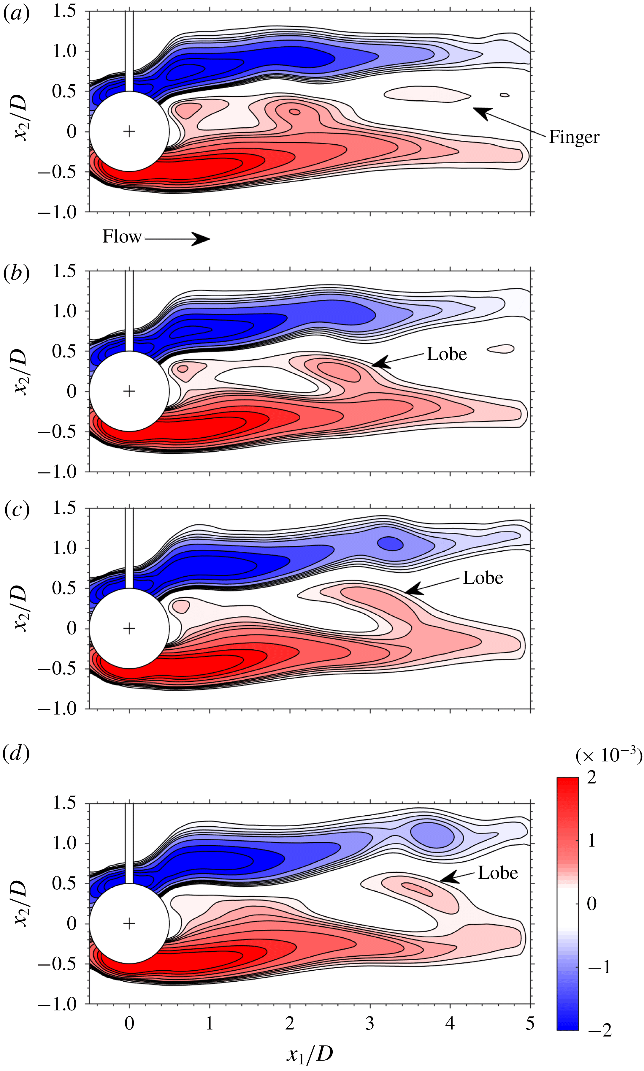
(a) 1.5, (b) 2.25, (c) 3.0 and (d) 3.75. Level list
 $\pm [0.3:0.1:0.7~1:0.5:2.5]\times 10^{-3}$
.

The temporal sequence of equatorial (
 $x_{1}{-}x_{2}$
) planes of
 $\overline{\unicode[STIX]{x1D714}}_{3}D/U$
depicted in figure 18 shows how the distribution of
 $\overline{\unicode[STIX]{x1D714}}_{3}$
changes as vortex shedding progresses. Positive
 $\overline{\unicode[STIX]{x1D714}}_{3}$
governs the near wake and at
 $tU/D=1.5$
(figure 18
a), a ‘finger’ of positive
 $\overline{\unicode[STIX]{x1D714}}_{3}$
extends downstream, similar to what was reported by Johnson & Patel (Reference Johnson and Patel1999). However, in addition a lobe of intense
 $\overline{\unicode[STIX]{x1D714}}_{3}$
is observed that becomes more pronounced as it is advected downstream. Just upstream of this lobe,
 $\overline{\unicode[STIX]{x1D714}}_{3}$
is strongly reduced as the secondary vortices are generated by transforming transverse vorticity components into the streamwise component.
Temporal sequence of 3-D iso-surfaces of
 $\overline{\unicode[STIX]{x1D714}}_{1}D/U$
projected onto the
 $x_{1}{-}x_{2}$
plane;
 $tU/D$
 $=$
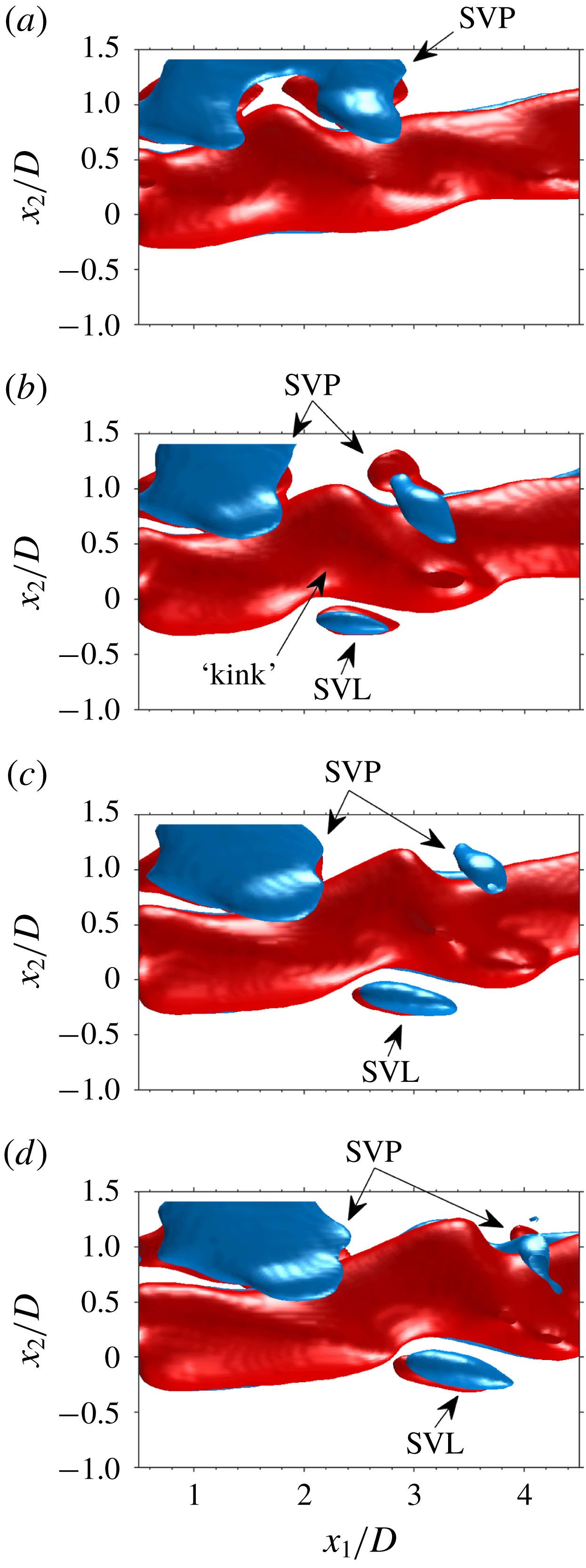
(a) 1.5, (b) 2.25, (c) 3.0 and (d) 3.75. Iso-surface levels are
 $1.03\times 10^{-4}$
(red) and
 $-1.03\times 10^{-4}$
(blue).

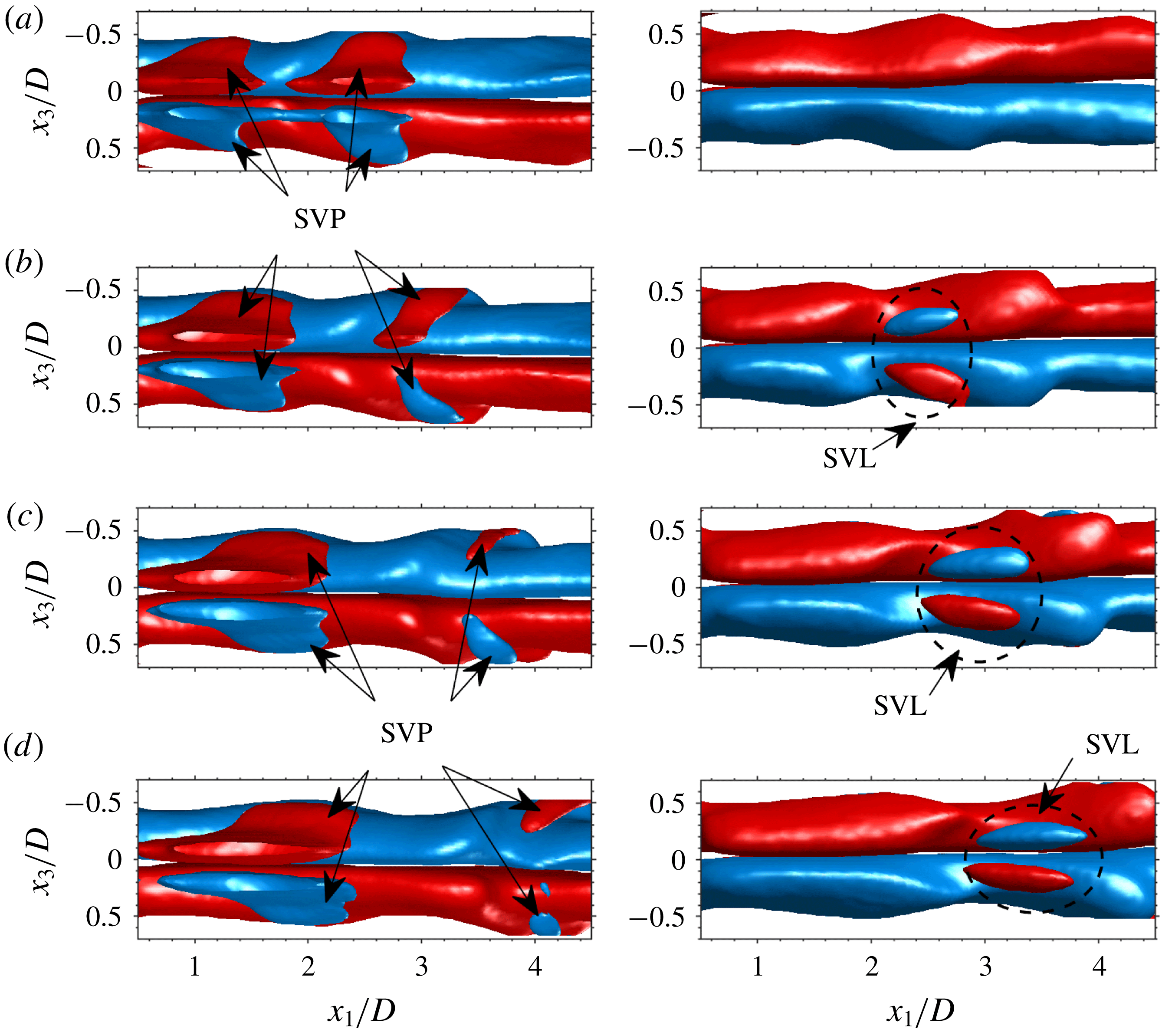
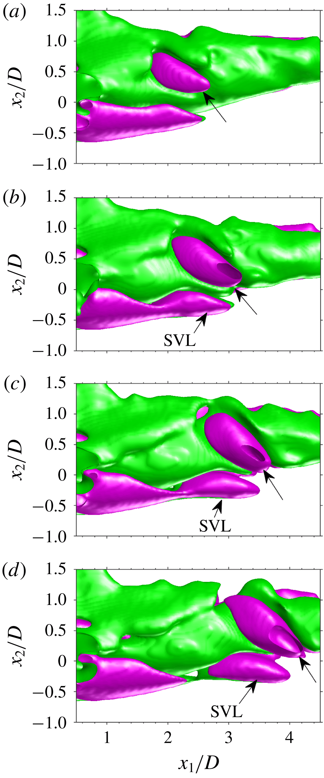
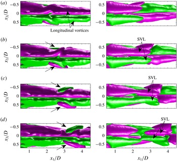
The three-dimensional topology of the streamwise vorticity component in the wake of the sphere is further illustrated in figures 19 and 20 by planar projections of iso-surface plots at different times in the vortex shedding cycle. The side and bottom views depicted in figures 19 and 20 (right column), respectively, clearly show that at
 $tU/D=2.25$
(figures 19
b, 20
b), the legs of the secondary vortex (‘SVL’) appear beneath those of the shed ‘hairpin’ head at
 $x_{1}/D\approx 2.5$
. The former grow slowly in streamwise extent as they are advected downstream. Note that although the ‘hairpin’ heads (top view in figure 20) are characterized by streamwise vorticity patches (SVP) ‘embracing’ the longitudinal vortices (figures 19
b and 20
c), our data never showed any connection between them and those of the equal sign legs of the secondary vortex (SVL), strengthening our results that the secondary vortex is generated by the action of the counter-rotating longitudinal vortices that become ‘kinked’ (figure 19
b) as the induced vortex is generated.
Temporal sequence of 3-D iso-surfaces of
 $\overline{\unicode[STIX]{x1D714}}_{1}D/U$
projected onto the
 $x_{1}{-}x_{3}$
plane;
 $tU/D$
 $=$
(a) 1.5, (b) 2.25, (c) 3.0 and (d) 3.75. Left and right columns depict top and bottom view, respectively. Iso-surface levels are
 $1.03\times 10^{-4}$
(red) and
 $-1.03\times 10^{-4}$
(blue).

Temporal sequence of 3-D iso-surfaces of
 $\overline{\unicode[STIX]{x1D61A}}_{1j}\overline{\unicode[STIX]{x1D714}}_{j}D^{2}/U^{2}$
projected onto the
 $x_{1}{-}x_{2}$
plane;
 $tU/D$
 $=$
(a) 1.5, (b) 2.25, (c) 3.0 and (d) 3.75. Iso-surface levels are
 $8.62\times 10^{-7}$
(green) and
 $-8.62\times 10^{-7}$
(purple). Arrows without text point at structures associated with the ‘hairpin’ head.

Temporal sequence of 3-D iso-surfaces of
 $\overline{\unicode[STIX]{x1D61A}}_{1j}\overline{\unicode[STIX]{x1D714}}_{j}D^{2}/U^{2}$
projected onto the
 $x_{1}{-}x_{3}$
plane;
 $tU/D$
 $=$
(a) 1.5, (b) 2.25, (c) 3.0 and (d) 3.75. Left and right columns depict top and bottom views, respectively. Iso-surface levels are
 $8.62\times 10^{-7}$
(green) and
 $-8.62\times 10^{-7}$
(purple). Arrows without text point at structures associated with the ‘hairpin’ head.

Further insight into the generation mechanism of the induced vortices can be deduced from looking at the streamwise component of the vortex stretching term that appears in the vorticity equation (Pope Reference Pope2000) given by:
 $$\begin{eqnarray}\frac{\text{D}\unicode[STIX]{x1D74E}}{\text{D}t}=\unicode[STIX]{x1D708}\unicode[STIX]{x1D6FB}^{2}\unicode[STIX]{x1D74E}+\unicode[STIX]{x1D74E}\boldsymbol{\cdot }\unicode[STIX]{x1D735}\boldsymbol{U},\end{eqnarray}$$
where
 $\text{D}/\text{D}t$
denotes the material derivative, the second term is vorticity diffusion by viscosity and the third term is the vortex stretching term. The latter can be shown to equal
 $\unicode[STIX]{x1D61A}_{ij}\unicode[STIX]{x1D714}_{j}$
(Panton Reference Panton2006). In the present work, we expect significant vortex stretching in the wake of the sphere as a result of the streamwise vortex stretching component when the secondary and shed primary vortices are created.
The temporal sequence of 3-D iso-surfaces of the streamwise component of the vortex stretching term,
 $\unicode[STIX]{x1D61A}_{1j}\unicode[STIX]{x1D714}_{j}$
, are shown as side and top/bottom views in figures 21 and 22, respectively. The 3-D topology has some similarities to the iso-surface plots of
 $\overline{\unicode[STIX]{x1D714}}_{1}D/U$
plotted in figures 19 and 20 but also several differences. Similar to
 $\overline{\unicode[STIX]{x1D714}}_{1}D/U$
, the distribution of
 $\overline{\unicode[STIX]{x1D61A}}_{1j}\overline{\unicode[STIX]{x1D714}}_{j}$
associated with the longitudinal vortices materializes as longitudinal structures aligned with the legs (see figure 22
a, top view). Both negative and positive
 $\overline{\unicode[STIX]{x1D714}}_{1}D/U$
are stretched by equally signed
 $\overline{\unicode[STIX]{x1D61A}}_{1j}\overline{\unicode[STIX]{x1D714}}_{j}$
. The patches of
 $\overline{\unicode[STIX]{x1D61A}}_{1j}\overline{\unicode[STIX]{x1D714}}_{j}$
associated with the ‘hairpin’ head (indicated by the arrows in figures 21 and 22
b–d, left column), are clearly observed at
 $tU/D=1.5$
and at the same time, elongated
 $\overline{\unicode[STIX]{x1D61A}}_{1j}\overline{\unicode[STIX]{x1D714}}_{j}$
‘lobes’ associated with the secondary vortex legs (denoted by ‘SVL’ in figures 21 and 22), develop at the bottom of the oppositely signed structures. As the ‘hairpin’ is advected downstream, these ‘lobes’ detach from the near-wake region as the secondary vortex develops further.
5 Summary and discussion
The instantaneous 3-D vortex structure in the wake of a stationary sphere at
 $Re=465$
has been measured using tomo-PIV. The results indicated that secondary vortices that appeared in the DNS of Johnson & Patel (Reference Johnson and Patel1999) as well as in the planar PIV measurements by Brücker (Reference Brücker2001) but were never seen in dye or smoke visualizations (e.g. Achenbach Reference Achenbach1974; Sakamoto & Haniu Reference Sakamoto and Haniu1990; Johnson & Patel Reference Johnson and Patel1999; Leweke et al.
Reference Leweke, Provansal, Ormieres and Lebescond1999) indeed exist. Combining the tomo-PIV with time-resolved planar PIV measurements together with vortex shedding periodicity at this
 $Re$
, the ensemble averaged vortex shedding cycle in the wake of the sphere was reconstructed. Strong shed primary vortices with their ‘hairpin’ heads always pointed in the same direction were shed from the near recirculating wake close to the sphere while counter-rotating longitudinal vortices extended from the near wake in the downstream direction at every stage of the shedding sequence. As the shed ‘hairpin’ head was advected downstream of the sphere, the interaction between the outer shear flow and the counter-rotating longitudinal vortices generates a secondary vortex by transforming transverse vorticity generated at the sphere into streamwise vorticity, and as a result a saddle point appears. The secondary vortex head emerged in the range
 $3.0<x_{1}/D<3.5$
, and was located below the shed ‘hairpin’ head in good agreement with the DNS by Johnson & Patel (Reference Johnson and Patel1999). Both were advected downstream. While the ‘legs’ of the secondary vortex were not clearly observed in the ensemble averaged shedding cycle based on the
 $Q$
-criterion, their generation was clearly observed in the 3-D iso-surface plots of the streamwise component of the vorticity and the vortex stretching term. In both cases, distinct opposite sign, elongated ‘lobes’ are observed prior to the appearance of the induced vortex head that was visualized by the
 $Q$
-criterion. As far as the authors are aware, these are the first spatially resolved, three-dimensional results that experimentally show the existence of the secondary vortices.
Acknowledgements
This research was partially supported by the Edmund J. Safra Philanthropic Foundation, the Wolfson Family Charitable Trust, the Technion Fund for Promotion of Research and the Israel Science Foundation under grant no. 1596/14.