Introduction
Benoit Mandelbrot (1924–2010) was a French and American mathematician (Fig. 1) who referred himself as “fractalist” [Reference Mandelbrot1] and is well recognized for his contribution to the field of fractal geometry, who coined the word “fractal” and developed the theory of “roughness and self-similarity” in nature. As a visiting professor at Harvard University, Mandelbrot began to study fractals called “Julia sets” based on previous work by Gaston Julia and Pierre Fatou. In 1982, he expanded his ideas in “The Fractal Geometry of Nature” [Reference Mandelbrot1] which brought fractals into the mainstream of professional and popular mathematics. His informal and passionate style of writing and his emphasis on visual and geometric intuition made “The Fractal Geometry of Nature” accessible to non-specialists which sparked widespread interest in fractals which is acceptable in almost every field from finance to physics to medicine.
Benoit Mandelbrot (Warsaw 1924–Cambridge 2010) considered as the father of Fractal Geometry [Wikipedia].

In the study of fractal structures, geometric series often arise as the perimeter, area, or volume of a self-similar structure. For example, the area of Koch snowflake [Reference Mandelbrot1] can be described as the union of infinitely many equilateral triangles (Fig. 2). Here, each side of the green triangle is exactly 1/3 the size of a side of the large blue triangle, and therefore has exactly 1/9 of the area. Similarly, each yellow triangle has 1/9 of the area of a green triangle, and so forth. Taking the blue triangle as a unit of area, the total area of the snowflake can be calculated as:

Geometry of a Koch snowflake [Reference Peitgen, Jurgens and Saupe2] [Wikipedia].

The first term of this series represents the area of the blue triangle, the second term represents the total area of the three green triangles, the third term represents the total area of the 12 yellow triangles, and so forth. Excluding the initial 1, this series is geometric with constant ratio r = 4/9. The first term of the geometric series is, a = 3(1/9) = 1/3, so the sum is:

Thus, the Koch snowflake has 8/5 of the area of the base triangle leading to convergent series formulation.
Also, perturbation theory can be used efficiently to obtain a prescription that recursively generates the structure of the abstract attracter. This technique can be used in the calculation of the fractal dimension of the attracter of certain two- or three-dimensional maps. Presently, significant attention is being paid for characterizing the deterministic chaotic behavior of dynamic systems. The idea of characterizing the fractal quality of chaotic attractors in light of dimension-like parameters can be traced back to the geometric approach presented by Mandelbrot [Reference Mandelbrot1].
Based on Set Theory, Iterated Function System (IFS) [Reference Peitgen, Jurgens and Saupe2,Reference Werner and Mittra3] is a method for constructing fractals which are self-similar in nature.IFS fractals are made up of the union of several copies of itself where each copy is being transformed by a function system. IFS is based on affine transformation series, “w” which is defined by:

Here real number coefficients (a, b, c, d, e, f) are responsible for the movement of fractal elements in space: a, d – scaling; b, c – rotation by φ 1, φ 2 angles with respect to axis of coordinating system; and e, f – linear translation by the vector (e, f) respectively. These coefficients are expressed as follows: a = δ 1cos φ 1, d = δ 2cos φ 2, b = δ 2sin φ 2, c = δ 1cos φ 1. A canonical example is shown in Fig. 3 which is called Sierpinski Gasket [Reference Mandelbrot1] that begins with a triangle and the middle piece is cut out as shown in the generator in Fig. 3. This results in three smaller triangles for which the process is continued. The nine resulting smaller triangles are cut in the same way and so forth, indefinitely. The gasket structure is perfectly self-similar, with an attribute of many fractal images where any triangular portion can be seen as an exact replica of the whole gasket.
Sierpinski gasket geometry till 4th iteration (0th, 1st, 2nd, 3rd, and 4th iteration) [Reference Peitgen, Jurgens and Saupe2].

L-systems introduced by Lindenmayer in 1968 [Reference Peitgen, Jurgens and Saupe2] is an albhabet based method which are used to describe the behavior of plant cells and to model the growth process of plant development. The recursive nature of L-system leads to self-similarity and fractal-like forms can also be described by L-systems. It is useful to create some fractals based on Hilbert and Peano curves.
A long-term effort by several researchers around the globe to combine fractal geometry with electromagnetic theory has led to a plethora of innovative antenna designs [Reference Peitgen, Jurgens and Saupe2,Reference Werner and Mittra3] which led to an era called fractal antenna engineering [Reference Werner and Ganguly4,Reference Werner5] which is primarily focused in two broad areas: the design of fractal antenna elements as well as the application of fractal to the design of antenna arrays. Fractal antenna geometries can be classified into two categories as deterministic and random. Random fractals are basically produced by the trajectories of non deterministic functions. Several studies on deterministic antenna structures for which the self-similarity property can be applied by a scaling factor have been carried out in this report. Several fractal geometries have been revisited for antennas with special characteristics, in the context of both antenna elements and spatial distribution functions for elements in antenna arrays.
In this review article, researches on fractal multiband antennas are summarized in section “Fractal antennas for multiband wireless applications”. Section “Fractal antennas for wideband applications” embodies summaries of fractal wideband antennas. In section “Fractal antennas for UWB applications”, fractal UWB antennas have been summarized and it concludes with a discussion on research trends in the field of fractal antenna arrays in section “Fractal array antennas”.
Fractal antennas for multiband wireless applications
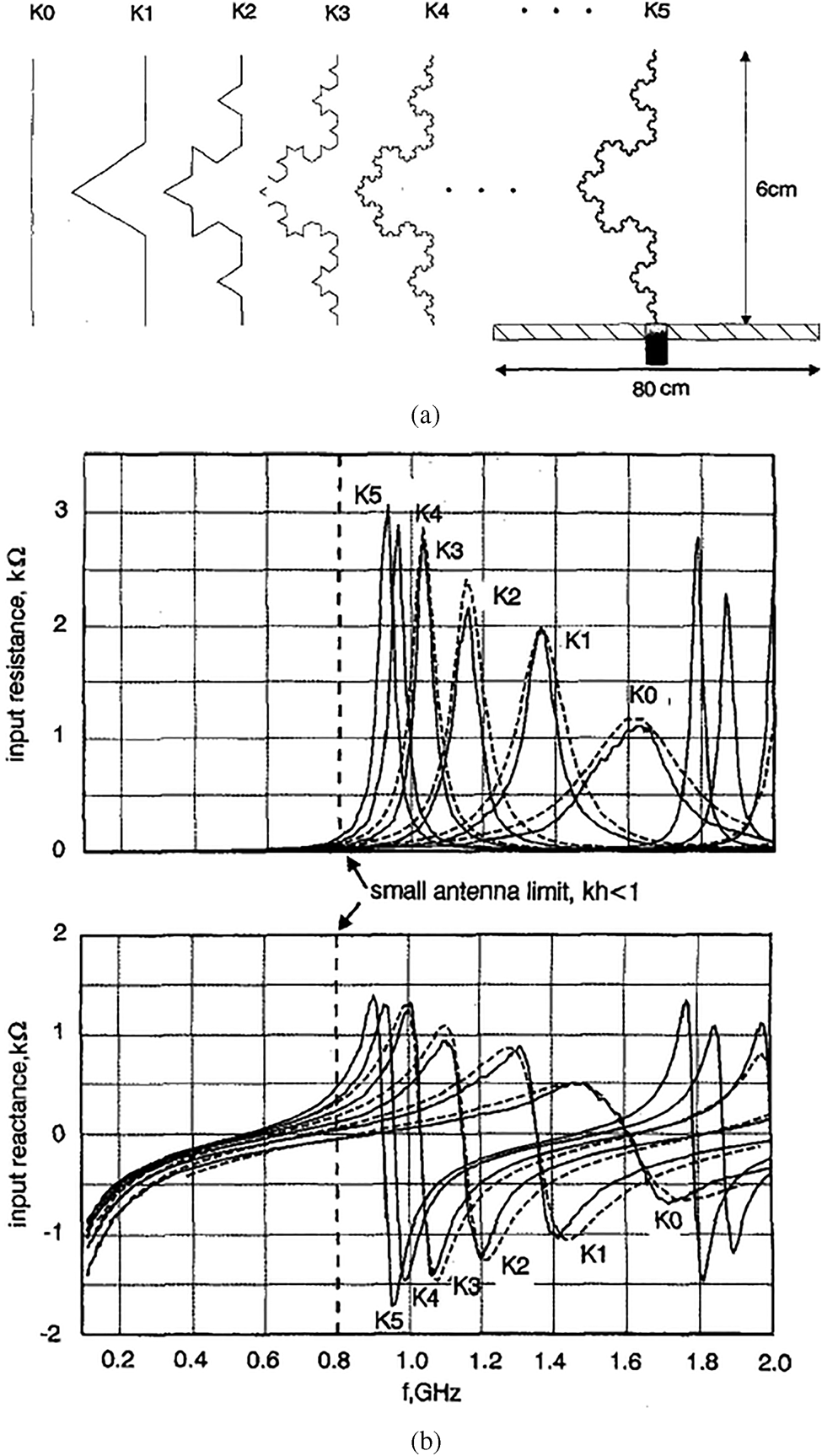
In modern scenario, a wireless device is often required to operate in more than one band of frequency. An antenna that covers multiple wireless communication bands is considered as a multiband antenna. This section revisited a few important works on fractal multiband antennas by various researchers. The application of fractal geometry for the design of wire antennas was first proposed in a series of articles by Cohen [Reference Cohen6–Reference Cohen11] which shows the fractalizing of the geometry of a standard dipole or loop antenna. Later, properties of Koch fractal monopole, investigated by Puente et al. in [Reference Puente, Romeu, Pous, Ramis and Hijazo12,Reference Puente, Romeu and Cardama13] have shown improved electrical performance over conventional linear monopole which is depicted in Fig. 4.
(a) Koch monopole antenna with various iterations. (b) Variation of input resistance and reactance with the frequency of the antenna for different iterations [Reference Puente, Romeu, Pous, Ramis and Hijazo12].
Monopole configurations with fractal top-loads have been considered here as an alternative technique for achieving size miniaturization. Puente et al. were the first to study a fractal two-dimensional (2-D) tree antenna which is inspired by a real tree where the top of every branch splits into more branches. It is seen that multiband behavior along with a denser band distribution than the Sierpinski antenna and the matched frequencies are found to be related to the length distribution over the fractal shape. Later, several antenna designs are considered [Reference Petko and Werner14] where fractal trees are shown to be as end-loads in order to miniaturize conventional dipole or monopole antennas (Fig. 5). Fractal antennas are not limited to only wire antennas rather it provides a medium which is easy to analyze and fabrication.
Fractal-tree dipole antennas [Reference Petko and Werner14].

In [Reference Rmili, Mrabet, Floc'h and Miane15], a random 3-D fractal antenna (Fig. 6) with an electrochemical deposition has been characterized by a monopole configuration. The novelty of this structure is the improvement of the impedance bandwidth compared to a similar 2-D fractal-tree antenna with less dense band distribution. In Fig. 6, fi represents different resonant frequencies throughout the operating band.
(a) Fractal-tree monopole antenna. (b) Measured return loss characteristics [Reference Rmili, Mrabet, Floc'h and Miane15].

Sierpinski triangle loop antenna with feed at the apex of the triangle [Reference Karami and Karami16] proposed by Karami and Karami, which has a radiation characteristic like a dipole. Electromagnetic characteristics of a Koch fractal antenna as an element and as an array are extensively examined by Deen et al. in [Reference Zainud-Deen, Awadalla, Khamis and El_shalaby17] using MoM (Method of Moments). Sierpinski fractal planar monopole [Reference Puente, Romeu, Pous, Garcia and Benítez18] antenna first reported by Puente et al. in 1996 which shows log periodic behavior in a single antenna itself with the number of resonances increasing with increasing iteration. Further studies on generalized antenna design based on Pascal Sierpinski gasket [Reference Romeu and Soler19] which are derived from Pascal triangle showed log periodic behavior. In [Reference Best20,Reference Best21], Best showed that the multiband characteristics of the Sierpinski gasket are basically a function of the periodic placement of the four gaps located along the central vertical axis of the antenna. It is concluded that the electromagnetic nature of Sierpinski gasket is a function of the periodic arrangement of the four gaps positioned along the central vertical axis of the antenna, which results in Parany gasket antenna. He further studied on Parany gasket antenna (Fig. 7) with perturbed gaps which showed identical allocation of frequency bands along with multiband behavior.
(a) Perturbed Parany gasket antenna. (b) S 11 characteristics compared to a conventional Sierpinski gasket monopole antenna [Reference Best20].

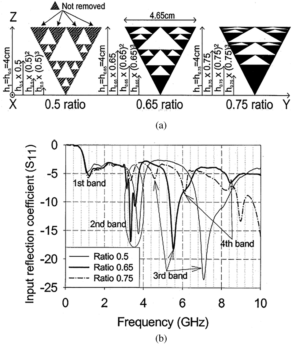
From the design point of view, mathematical expressions given in [Reference Mishra, Ghatak and Poddar22] for the calculation of the frequencies of resonance of the Sierpinski gasket are found necessary. It is seen that multiple ring monopoles [Reference Song, Hall, Ghafouri- Shiraz and Wake23,Reference Song, Hall and Ghafouri-Shiraz24] have similar characteristics to the Sierpinski gasket monopole antenna. When the circular shape is changed to an elliptic, there is an improvement in the bandwidth and radiation properties. From the return loss plots, it is observed that the impedance bandwidth increases for higher resonance and the lower ones are not prominent. Perturbed Sierpinski gasket monopole antenna studied by Song et al. [Reference Song, Hall and Ghafouri-Shiraz25] is extensively studied for overcoming the matching difficulties of a perturbed Sierpinski gasket fractal antenna (Fig. 8). These techniques enables multiband matching to a conventional 50 Ω SMA connector, without using any kind of matching circuits. A methodology for reducing the frequency separation between the first and second band of these triangular antennas has also been proposed. Based on Sierpinski gasket, a design for a triple-frequency broadband antenna based on a hybrid technique that combines a mono-band as well as dual-band broadband MPAs has been presented [Reference Anguera, Martandiacute, Puente, Borja and Soler26]. In [Reference Hwang27], a perturbed Sierpinski fractal patch with slotted ground plane is employed in a modified version to achieve dual broadband characteristics which is shown in Fig. 9. The proposed antenna has two operational bands (808–1008 and 1581–2760 MHz) covering GSM/DCS/PCS/ IMT-2000/ISM/satellite DMB services.
(a) A perturbed Sierpinski monopole. (b) Corresponding S 11 characteristics [Reference Song, Hall and Ghafouri-Shiraz25].
(a) Modified Sierpinski fractal patch with a slotted ground plane. (b) Simulated and measured S 11 characteristics of the antenna with fabricated prototype (ah = 5 mm, aw = 25 mm, s = 8.7 mm, w 1 = 1 mm, w 2 = 1 mm, l 1 = 20 mm, l 2 = 28 mm) [Reference Hwang27].

An RF MEMS reconfigurable fractal antenna [Reference Kingsley, Anagnostou, Tentzeris and Papapolymerou28] on a flexible organic polymer substrate for multiband applications has been reported which operates at several different frequencies between 4 and 18 GHz. Here, three sets of RF MEMS (microelectromechanical systems) switches with different actuation voltages are used to sequentially activate as well as deactivate parts of a multiband Sierpinski gasket which allows direct actuation of the electrostatic MEMS switches through the RF signal feed. The antenna structure and measured S 11 characteristics are shown in Fig. 10.
(a) MEMS reconfigurable Sierpinski antenna. (b) Measured return loss characteristics of the proposed antenna [Reference Kingsley, Anagnostou, Tentzeris and Papapolymerou28].

A dual-band fractal monopole antenna for handheld devices is proposed in [Reference Hwang29] where a modified half-Sierpinski gasket is used in the patch to cover two wideband frequencies with bandwidths of 55% (1517–2670 MHz) and 16% (5135–5828 MHz) which is shown in Fig. 11.
Simulated and measured S 11 characteristics of perturbed Sierpinski gasket monopole [Reference Hwang29].

A compact modified Sierpinski gasket monopole antenna with the ability to allocate both the 4 and 5.2 GHz ISM bands without a matching network is presented in [Reference Tsachtsiris, Soras, Karaboikis and Makios30]. Another modification of Sierpinski gasket (Fig. 12) is presented in [Reference Krzysztofik31] where a significant size reduction is seen than a traditional Sierpinski gasket by controlling the space factor between the first two resonances. Results show that locating an internal antenna at the rear of the mobile handset minimizes radiation pattern alteration as well as gain depression due to the proximity of human tissue. It has an ability to handle both 4 and 5.2 GHz ISM bands without a matching network.
(a) Numerical and physical model of the antenna [All dimensions are in 'mm']. (b) Simulated and measured S 11 characteristics of the antenna [Reference Krzysztofik31].

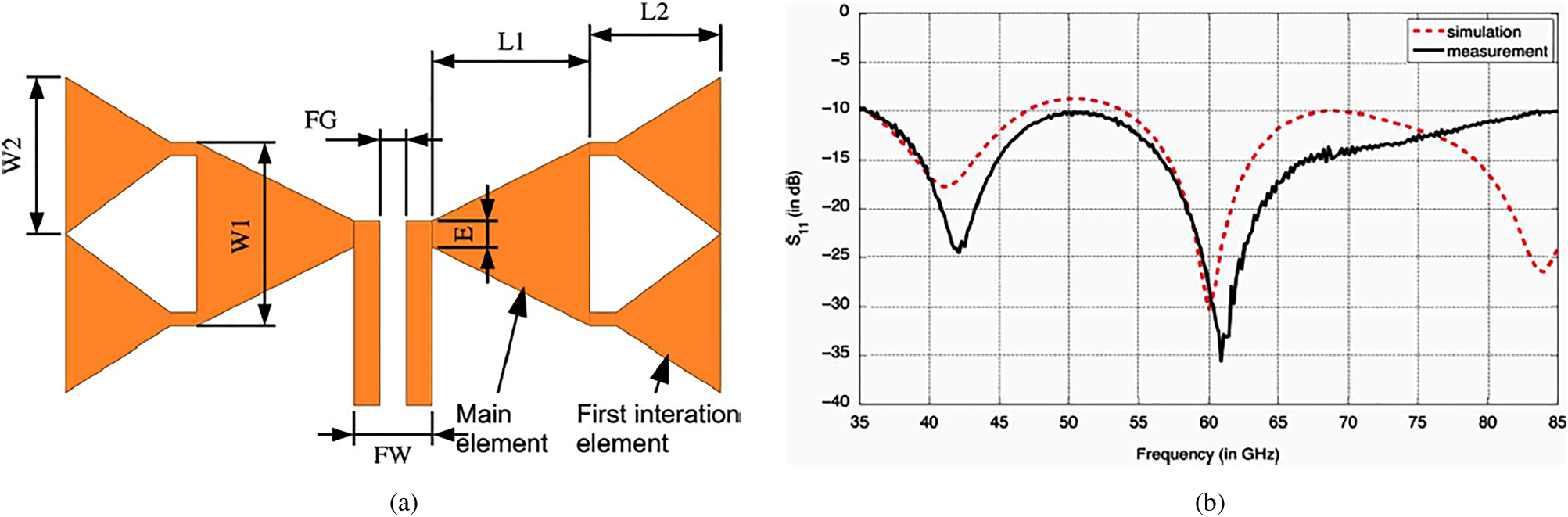
A dual-band compact PIFA (planar inverted-F antenna) implemented [Reference Soh, Vandenbosch, Ooi and Husna32] using the conductive textile shield is proposed for wearable application. The antenna can be used both in the 45 GHz and in the 5.2 GHz bands with omnidirectional radiation characteristics with a measured gain of about 3.1 dBi. Based on first iterative fractal bowtie antenna design, recently a new buckled cantilever plate-based on-chip compact dual-band (60and 77 GHz) antenna [Reference Marnat, Carreno and Conchouso33] using a CMOS compatible MEMS process has been proposed for efficient mm-wave applications (Fig. 13). It is vertically positioned with respect to the silicon substrate for better efficiency as compared to the horizontal position. An improved gain of 6 dB has been observed in simulation as well as in the measurement process of the antenna.
(a) Antenna geometry (L1 = 695 μm, L 2 = 818.3 μm, W 1 = 600 μm, W 2 = 760 μm, E = 25μm, FW = 60 μm, FG = 10 μm). (b) S 11 characteristics of the proposed antenna [Reference Marnat, Carreno and Conchouso33].
Another fractal geometry, which is well discussed by researchers in fractal antenna paradigm, is the Sierpinski carpet fractal (SCF). The SCF volume microstrip patch antenna is reported in [Reference Walker and James34] along with stacked SCF antenna over EBG (electromagnetic bandgap (EMBG)) ground plane. A multiband SCF antenna using transmission line feed is reported [Reference Rahim, Abdullah and Aziz35] with an impedance bandwidth of 47.1% at the resonant frequency of 7.93 GHz. In [Reference Ghatak, Mishra and Poddar36], a perturbed SCF planar antenna with CPW feed suitable for IEEE 8011a and 8011b lower and mid bands as well as for HiperLAN2 system is presented which is shown in Fig. 14. Another SCF patch antenna [Reference Li, Khan, Liu and He37] with a slant strip in the first iteration is proposed for dual WLAN application. A fractal PIFA based on SCF is presented in [Reference Saidatul, Azremi, Ahmad, Soh and Malek38] for mobile phone application. A printed dipole antenna [Reference Ooi and Selvan39] based on SCF has been reported for dual-band application with impedance bandwidths of 38.6 and 4.7% centered at 1.1 and 3 GHz. A novel microstrip patch antenna with a Koch prefractal edge and a U-shaped slot is presented [Reference Guterman, Moreira and Peixeiro40] for multi-standard application in GSM1800, UMTS, and HiperLAN2. It is implemented in PIFA configuration with a size reduction of 62% (Fig. 15).
(a) Dimension of the proposed antenna [g = 1 mm, Lg = 184 mm, h = 1.743 mm, Wg = 20.5 mm]. (b) Corresponding S 11 characteristics [Reference Ghatak, Mishra and Poddar36].

(a) Koch curve fractal patch antenna with fabricated prototype in inset [All dimensions in 'mm']. (b) S 11 characteristics of the antenna [Reference Guterman, Moreira and Peixeiro40].

Taking the advantage of Koch profile, a dual-band antenna [Reference Anguera, Puente, Borja and Soler41] is presented using reactive loading where the bandwidth is enhanced using a stacked parasitic technique. Another CPW-fed modified Koch fractal printed slot antenna is presented [Reference Krishna, Gopikrishna, Anandan, Mohanan and Vasudevan42] for dual wideband characteristics suitable for WLAN and WiMAX. Here, the introduction of a Koch fractal slot lowers the frequency of operation along with wide-band matching. In [Reference Ghatak, Poddar and Mishra43], input impedances and radiation characteristics of half-wavelength Koch fractal V-electric dipoles having included angles 60°, 90°, and 120° have been discussed. Recently in [Reference Fazal, Khan and Ihsan44], the introduction of partial Koch fractal boundaries to a traditional triangular patch results in antenna designs with high gain, low side lobe levels, and improved return loss. In [Reference Li and Mao45], a Koch-like sided fractal bowtie dipole is presented which can operate in multiband as well as ultra-wideband regime depending upon notch angle φ. When this angle increases in the range 0°–90°, UWB transform into multiband gradually. Another tri-band antenna [Reference Zhou, Luo, You and Yan46] which is end-loaded with Koch fractal loops is reported for radio frequency identification (RFID) applications. In [Reference Jalil, Abd Rahim, Samsuri, Murad, Majid, Kamardin and Azfar Abdullah47], a multiband Fractal Koch dipole textile antenna is proposed for wearable applications.
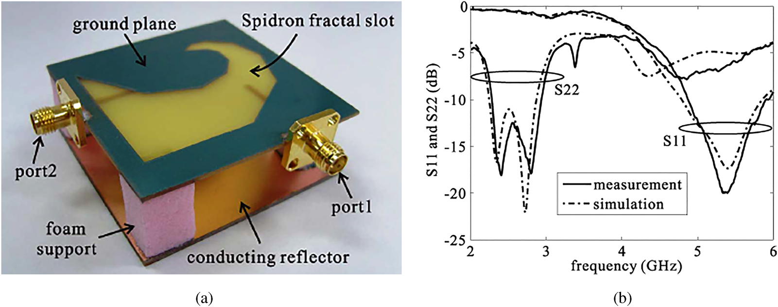
Slot antennas in fractal domain are attracting much more attention in recent times. In [Reference Sayem and Ali48], a third-order Hilbert slot antenna is reported with dual-resonance characteristics with a much smaller size to a printed half-wave dipole or full-wave slot antenna. Using Descartes circle theorem (DCT), a CPW-fed circular fractal slot antenna [Reference Chang, Zeng and Liu49] is proposed for dual-band applications. In [Reference Kim and Hwang50], a novel Spidron fractal slot antenna consists of a Spidron fractal slot, two microstrip feeding lines and a conducting reflector developed for multiband gap-filler application (Fig. 16). Here, two microstrip feeders are used to excite the Spidron fractal slot antenna at the 5 and 5.5 GHz frequency bands.
(a)Fabricated Spidron fractal slot antenna. (b) Corresponding return loss characteristics. [Reference Kim and Hwang50].
Some other types of fractal antennas are reported in [Reference Tang and Wahid51], where a novel hexagon fractal corner-fed patch antenna in dipole configuration is analyzed that showed multi-band characteristics. A new type of fractal microstrip patch antenna named as the crown square fractal antenna is studied in [Reference Dehkhoda and Tavakoli52]. Apart from showing multi-band characteristics and size reduction when compared to a near square patch antenna, these antennas are claimed to exhibit a pair of circularly-polarized bands in a wide VSWR bandwidth at high-frequency modes. A dual-band monopole antenna operating in the L1 and L2 GPS bands is presented in [Reference Azaro, Natale, Donelli, Zeni and Massa53]. The Kock prefractal antenna has been synthesized by means of a PSO for optimizing the values of the electrical parameters within the specifications. An alternative multiband approach [Reference Liu, Wu, Chen, Chang and Chen54] using Descartes theorem is presented for constructing a modified Sierpinski fractal monopole antenna where the resonances exhibit log periodic behavior. With increasing frequency, the patterns have an increasing number of lobes that exhibit array characteristic. Based on the Descartes theorem and non-constant fractal ratio, the multi-band performances of compound log-periodic Apollonian packing monopole antennas are presented in [Reference Liu, Wu, Chang and Liu55]. A triple-band patch antenna [Reference Azaro, Zeni, Rocca and Massa56] working in E5-L1 Galileo and WiMAX frequency bands is presented where the geometry of the antenna is defined by a Koch-like erosion in a Euclidian patch structure according to a Particle Swarm strategy.
A new type of fractal antenna [Reference Sinha and Jain57] called hybrid fractal has been reported for multiband application which behaves similarly to the Sierpinski gasket, repeating its resonant frequencies by a factor of two. A rectangular fractal dipole antenna with two operating bands for RFID is presented in [Reference Lee and Sun58]. By using a fractal slot and metal meander patch, the proposed antenna has wideband as well as dual return loss characteristics. A multi-band Cantor fractal monopole antenna covering GSM, DCS, PCS, UMTS, and WLAN applications have been presented in [Reference Manimegalai, Raju and Abhaikumar59]. In [Reference Ghosh, Sinha and Kartikeyan60], several dual-band cavity-backed fractal aperture antennas are investigated where the problem formulation is done by using a hybrid finite element-boundary integral method. A triangular monopole antenna [Reference Gemio, Granados and Castany61] on Sierpinski gasket fractal-based ground plane is proposed to obtain a dual-band characteristic for the 8011 standard (WLAN). It is observed that this fractal-based ground plane introduces new matched bands and can improve the existing ones. Based on real coded genetic algorithm in conjunction with electromagnetic simulations, a novel technique [Reference Ghatak, Poddar and Mishra62] for designing Sierpinski gasket fractal microstrip antenna is proposed. This method determines the side-length and the fractal iteration number of the antenna for the operations at 4.56, 7.51, and 11.78 GHz frequency bands. A monopole quad-band antenna based on a Hilbert self-affine prefractal geometry has been proposed in [Reference Azaro, Viani, Lizzi, Zeni and Massa63]. An innovative design of fractal monopole-like antenna [Reference Bor, Lu, Liu and Zeng64] with five series of Hilbert-curve configuration is proposed for IEEE 8011a/b/g WLAN as well as circular polarization applications. A miniaturized triple-band planar antenna working in GSM and Wi-Fi frequency bands is described in [Reference Azaro, Debiasi, Zeni, Benedetti, Rocca and Massa65] where a hybrid pre-fractal shape is obtained by integrating a Sierpinski and a Meander-like structure. A 2-D irregular fractal-jet printed antenna originated from a real image of a fractal jet fluid is designed [Reference Rmili, Floch and Zangar66] and characterized for 1–30 GHz multiband behavior. A modified fractal rhombic patch monopole multiband antenna [Reference Mahatthanajatuphat, Saleekaw and Akkaraekthalin67] has been proposed for multiple wireless communication system. Here, a modified ground plane has been employed to improve input impedance bandwidth and high-frequency radiation characteristics. Another compact printed RFID dipole antenna is proposed [Reference Kimouche, Zemmour and Atrouz68] which consist of different combination of fractals with the aim of reducing antenna size. For the matching purpose with the essentially complex impedance of the electronic chip directly embedded into the radiator, a double T-match structure is used. Another hybrid design of a compact ring fractal monopole antenna [Reference Pourahmadazar, Ghobadi, Nourinia and Shirzad69] with semi ellipse ground plane is proposed for modern mobile devices having WLAN as well as WiMAX applications. By increasing the fractal iterations, very good impedance characteristics are obtained. A trapezoid monopole antenna [Reference Hong, Gong, Liu and Jiang70] with quasi-fractal slotted ground plane is applied for dual-frequency applications where the dual operating bands of the antenna are determined by the sizes of the radiator as well as the quasi-fractal structure (Fig. 17).
Simulated and measured S 11 characteristics of the antenna [Reference Hong, Gong, Liu and Jiang70].

Here, quasi-fractal slotted ground plane is applied to improve the dual-band characteristics of the antenna. A compact dual-band circular polarized fractal antenna consists of a Hilbert-curve and self-complementary configuration is presented in [Reference Liu, Zeng, Chen, Bor and Chang71]. This design combines the inductively loaded monopole antenna and the self-complementary antenna to obtain a new monopole antenna configuration. The Hilbert curve with a longer strip line determines the lower band of 43 GHz and the Hilbert curve with shorter strip line decides the higher band of 5.35 GHz. It is seen that by appropriately choosing the fractal properties [Reference Vinoy and Pal72], the design of a dual-frequency microstrip ring antenna using Minkowski curves can be done. A star-shaped fractal patch antenna is presented in [Reference Thakare and Kumar73] for miniaturization and backscattering radar cross-section reduction. A compact multiband third iterative E-shape fractal patch antenna [Reference Bayatmaku, Lotfi, Azarmanesh and Soltani74] has been proposed for multiband application to achieve size reduction as well as to enhance the number of operating bands. This antenna operates on LTE/WWAN (GSM850/900/1800/1900/UMTS/LTE2300/2500) band. A procedure [Reference Eichler, Hazdra, Capek, Korinek and Hamouz75] of planar antenna design using modal methods has been provided where the information about motif behavior is presented. By this method, it is possible to effectively analyze even complicated shapes like fractals. Here, the physical behavior of a planar antenna has been explained by modal decomposition along with a design of patch feeding and a full-wave analysis. It is seen that modal radiation patterns could successfully predict antenna radiation characteristics such as polarization or main lobe direction.
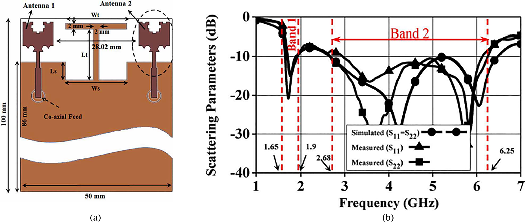
A design procedure is presented in [Reference Patnaik and Sinha76] for making custom-made fractal antennas using artificial neural networks and the particle swarm optimization (PSO) considering Sierpinski gasket and Koch monopole antennas. Based on a perturbed planar Sierpinski fractal shape, a dual-band monopole antenna suitable for Long Term Evolution (LTE) standard is proposed in [Reference Lizzi and Massa77] where the antenna geometry has been determined by means of a PSO. A compact modified Minkowski fractal loop monopole [Reference Chaimool, Chokchai and Akkaraekthalin78] antenna is proposed for USB dongle applications which cover Wi-Fi (4–484 and 5.15–5.35 GHz) and WiMAX (5–7 and 3.4–3.6 GHz) applications. Another compact microstrip antenna with a combination of square and Giuseppe Piano fractals [Reference Oraizi and Hedayati79] has been proposed for multiband operation along with circular polarization. Good axial ratio (AR) and radiation patterns prove the effectiveness and suitability of the proposed approach for wireless applications. A dual-band antenna obtained by replacing a segment of a square ring microstrip antenna with fractal Minkowski curve is studied in [Reference Behera and Vinoy80]. By increasing the indentation factor of the fractal radiator, the resonance frequencies of the antenna can be changed and by suitably optimizing this value, antenna can be designed with improved bandwidth with good gain at both the resonance frequencies. A dual-band microstrip RFID reader antenna [Reference Liu, Xu and Wu81] with tree-like fractal resonator is designed with 4.4 and 3.1% BW, respectively. Tri band RFID antennas [Reference Varadhan, Pakkathillam, Kanagasabai, Sivasamy, Natarajan and Palaniswamy82] are proposed for RFID reader as well as RFID tag for using in logistics management, traffic toll collection, and tagometry. Based on Minkowski island curve and Koch curve fractals, a hybrid fractal planar monopole MIMO antenna (Fig. 18) has been presented in [Reference Choukiker, Sharma and Behera83] which provides band widths of 14% for band-1 (1.65–1.9 GHz) and 80% for band-2 (68–6.25 GHz).
(a) Geometry of the proposed antenna. (b) Simulated scattering parameters of the antenna [Reference Choukiker, Sharma and Behera83].

A pseudo-self-complementary four-stage Parany monopole with side triangular complements and side-notched vertices has been proposed in [Reference Barroso, Mata and Diaz84] for multiband applcations. This antenna has a smaller physical area and length than the traditional Parany monopole. In [Reference Cai, Wang, Zhang and Shi85] a compact low-profile circularly-polarized (CP) antenna has been examined based on the combination of fractal metasurface and fractal resonator. A CPW-fed multiband fractal slot antenna [Reference Dhar, Patra, Ghatak, Gupta and Poddar86] loaded with a dielectric resonator for multiband wireless applications is proposed. Here the Minkowski fractal geometry is used to generate multiband behavior as well as helped in miniaturization than its Euclidian counterpart. In [Reference Farswan, Gautam, Kanaujia and Rambabu87], a circularly-polarized compact microstrip antenna using Koch fractal geometry for UHF RFID system is presented. A novel DRAF geometry is introduced in [Reference Orazi and Soleimani88] and implemented on an equilateral triangular patch for antenna miniaturization while keeping the bandwidth of the antenna constant. In [Reference Ratilal Prajapati, Gopala Krishna Murthy, Patnaik and Venkata Kartikeyan89], it is seen that the use of fractal DGS in the design of L-band planar antennas gives better antenna performance as compared with antennas without DGS (defected ground structure) and antennas with traditional DGS. In [Reference Taghadosi, Albasha, Qaddoumi and Ali90], a multiband antenna has been proposed to function as a receptor element in radio-frequency energy harvesting applications. In [Reference Velan, Sundarsingh, Kanagasabai, Sarma, Raviteja, Sivasamy and Pakkathillam91], the design of a dual-band wearable fractal-based monopole patch antenna integrated with an EBG structure is presented which covers the GSM-1800 and ISM-2.45 GHz bands. A multiport sharing compact antenna is presented in [Reference Wang, Wang, Gong and Ding92] where the radiator is composed of two Sierpinski fractal triangles. These two main ports have the operating band of 1–4 GHz where the auxiliary port with a multiband at around 2.4, 3.4, and 5.2 GHz provides an additional WLAN/WiMAX port. In [Reference Alibakhshi-Kenari, Naser-Moghadasi, Ali Sadeghzadeh, Virdee and Limiti93], a novel single-radiator card-type tag antenna is proposed using a series of Hilbert-curve loop and matching stub for HF/UHF dual-band RFID application. By merging the series Hilbert-curve HF coil along with square loop UHF antenna, a single radiator of RFID tag is obtained that meets the requirement of compactness and HF/UHF dual-band operation as shown in Fig. 19.
(a) Geometry of the proposed antenna. (b) Return loss characteristics of the antenna [Reference Alibakhshi-Kenari, Naser-Moghadasi, Ali Sadeghzadeh, Virdee and Limiti93].

In [Reference Wang, Wang and Li94], a sensor for a Moore fractal antenna is proposed to detect partial discharge (PD) in gas-insulated substations that can work at an ultra-high frequency. In [Reference Kgwadi and Drysdale95] a low-cost, frequency-agile triangular Sierpesnki gasket-based antenna is proposed for use by wireless sensor nodes in IoT applications. The antenna consists of PIN diodes, inductors as well as a single bias line to switch between two modes of operation. By switching the diodes on or off, the desired frequency agility between UHF (800 MHz) and the WLAN band (2400–2500 MHz) is achieved with corrosponding bandwidths of 200 and 1000 MHz, respectively. The concept called additive manufacturing techniques for the fabrication of 3-D fractal monopole antennas is presented in [Reference Jun, Sanz-Izquierdo, Parker, Bird and McClelland96]. The 3-D designs based on the Sierpinski fractal concept is studied and discussed. In [Reference Wei, Li, Wang, Xu and Xing97], a single-feed circularly-polarized antenna is presented where the CP radiation is achieved by adjusting the dimension of the fractal defected ground structure (DGS). In [Reference Chuma, de la Torre Rodríguez, Iano, Bravo Roger and Sanchez-Soriano98], a rectenna topology is presented by using a compact fractal patch antenna with the rectifier circuit that is integrated into the same physical structure suitable for harvesting and wireless power transfer applications. In [Reference Anguera, Andújar, Benavente, Jayasinghe and Kahng99], a single patch antenna is proposed to achieve the same directivity as an array with an equivalent area but without using the complex feeding network. In [Reference Braham Chaouche, Messaoudene, Benmabrouk, Nedil and Bouttout100], a CPW-fed reconfigurable antenna using crescent-shape fractal geometry is presented where the frequency reconfigurable approach is obtained by using RF PIN diodes, resistor, and inductors. The design allowed the reconfigurable switching up to eight frequency bands between 1.46 and 6.15 GHz. In [Reference Goswami, Ghatak and Poddar101], a novel multi-band microstrip line-fed metamaterial-based bisected Hilbert curve monopole antenna is designed with operating bands at WLAN 2.4, 5.8 GHz, Wi-max 3.5, 5.5 GHz, and RFID 5.2 GHz. In [Reference Mohammad Husain Ranjbaran and Mohanna102], an spiral antenna with a new fractal reflector for short-range sensing has been proposed to improve some features of the equiangular and Archimedean spiral antenna.
In [Reference Sharma, Lakwar, Kumar and Garg103], it is shown that SRRs can be applied for better impedance matching which can improve the bandwidth of a fractal antenna. This theory is successfully verified by designing a multiband circular fractal antenna which is loaded with SRRs, and the results have been compared for both the cases. The antenna shows improved impedance matching at all resonant frequencies. In [Reference Abed, Jit Singh and Islam104], for the proposed fractal antenna at each stage, a new modified square patch with a half size of that used in the previous stage is added to shape the dual fractal-structure antenna which is shown in Fig. 20.
(a) Configuration of the proposed antenna. (b) Return loss characteristics of the antenna [Reference Abed, Jit Singh and Islam104].

The antenna has dual-band characteristics that meet the specifications of the wireless fidelity Wi-Fi and WiMAX applications. The antenna also achieved an AR bandwidth (3 dB) which is 35% of the first operating band and 30% of the second operating band. In [Reference Elwi, Asaad Abdul Hassain and Almukhtar Tawfeeq105], an investigation is conducted on Hilbert metamaterial printed antenna to realize the possibility of organic materials usability in radio frequency (RF) electronics for RF-energy harvesting. A complementary stacked patch antenna based on Sierpinski fractal is introduced in [Reference Ghatak, Mishra and Poddar106] where it is seen that this new complementary structure enhances the antenna performances, retaining the basic characteristics of the Sierpinski antenna. Stacked patch antenna is proposed in [Reference Tiwari and Kartikeyan107] where fractal shaped defects have been etched from the patch surfaces which produce dual-band characteristics as well as size reduction. Based on Sierpinski gasket fractal, an electromagnetically coupled multilayer equilateral triangular stacked patch antenna is proposed in [Reference Malik and Kartikeyan108] for dual-band characteristics. Another stacked patch antenna consisting of a second iteration Minkowski-island-based (MIB) fractal patch is presented [Reference Hung, Liu, Bor and Chen109] for unidirectional radiation applications with 39.1% size reduction. It produces AR band width of 44 GHz. Based on complementary MIB fractal geometry, an aperture coupled stacked fractal patch antenna [Reference Hung, Liu, Wei, Chen and Bor110] has been presented with circular polarization. Dual-band responses at 3.5 and 5.25 GHz are obtained with 3 dB AR bandwidths of 1.4 and 0.76%.
In this section, we have provided an overview of recent developments on fractal multiband antennas where it is evident that several fractal geometries can be efficiently explored for antennas with multiband applications because a fractal can fill the space occupied by the antenna in a more effective manner than traditional Euclidian antennas that leads to more effective coupling from feed to free space in less volume.
Fractal antennas for wideband applications
The demand for today's wireless communication systems is not only a compact antenna but also an antenna with a large band width to provide several services in a single device. Wideband antennas can cover sufficiently large operating frequency bandwidth for many applications with a relatively large form factor. It is seen that besides achieving miniaturization and multiband nature, fractal concept can also be effectively explored to achieve wideband characteristics.
Using the concept of DCT [Reference Liu, Chang, Soong, Chen, Wu and Yao111] and self-similar iteration design; circular fractal antennas are proposed which exhibit frequency-independent characteristics and multiband spectra. In [Reference Lee112], a new uniplanar self-similar structured wideband loop antenna is presented where by alternating an inverted matrix sequence, wide impedance bandwidth has been obtained from 2 to 20 GHz for VSWR <5. Another novel wideband and compact fractal Kokh antenna is proposed [Reference Mirzapour and Neyestanak113] which has smaller size and wideband behavior respect to similar fractal Kokh antenna designs. The proposed antenna is able to achieve an impedance bandwidth of 19% for VSWR <2. . A compact wideband snowflake fractal antenna is proposed where various iterations with probe feed and capacitive coupled feed are compared and an optimized design is presented in [Reference Mirzapour and Hassani114]. It is shown that, with an air-filled substrate and capacitive feed, an impedance bandwidth up to 49% can be obtained. A planar Koch fractal loop antenna with broadband characteristics is presented in [Reference Patnam115] where the CPW feed along with radial stub makes the antenna completely planar which can be integrated with other microwave circuits. In [Reference Naghshvarian-Jahromi116], a new planar fractal antenna using third iterative Penta-Gasket-Koch (PGK) has been introduced where the matching performance of planar PGK has been compared with that of conventional PGK monopole antenna. This design achieved a good input impedance match and linear phase throughout a wide operating band of 1.5–20 GHz (<−5 dB) along with satisfactory time-domain performance. A broadband circularly-polarized fractal antenna [Reference Hwang117] is proposed (Fig. 21) where the concept of a novel Spidron fractal is employed to achieve both broadband as well as circular-polarization characteristics.
Simulated and measured return loss of the antenna [Reference Hwang117].

Printed slot antenna with a fractal-shaped square wide slot for bandwidth enhancement is proposed in [Reference Chen, Wang and Zhang118] where the impedance bandwidth is 3.5 times that of the corresponding conventional printed microstrip line-fed wide-slot antenna. It is shown that the proper selection of iteration factor and iteration order of the fractal shape improves the impedance bandwidth significantly (Fig. 22).
(a) Geometry and dimension of the proposed slot antenna. (b) Measured S 11 characteristics at different iterations [Reference Chen, Wang and Zhang118].

Sierpinski carpet (SC)-based square monopole antenna [Reference Anguera, Daniel, Borja, Mumbru, Puente, Leduc, Sayegrih and Van Roy119] has been designed using the possibilities of the metalized foam technology. In terms of impedance bandwidth, the reflection coefficient is <−7.7 dB from 824 MHz up to more than 6 GHz having a total average efficiency of 79%. In [Reference Naghshvarian Jahromi, Falahati and Edwards120], a compact second iteration SC fractal shape antenna is presented with the combination of the planar CPW-fed and the conventional monopole-fed antennas. This technique can provide a very good improvement in parameter magnitude considering SC geometry throughout the 4.65–10.5 GHz band pass. In [Reference Sung121], a Sierpinski fractal-shaped slot is employed for a wideband operation covering from 1.96 to 3.78 GHz. Here, the lower edge of the operating frequency band of the slot antenna is lowered by the fractal technique which results in a compact design. Another wideband antenna operating in a portion of the L-band frequency range is presented in [Reference Caramanica122] which is based on a Julia prefractal geometry and also optimized by means of hybrid-coded genetic algorithm to minimize size and VSWR ratio. A new fractal patterned iris-loaded cross dipole slot antenna along the broad wall of a rectangular waveguide at X-band is presented in [Reference Ghatak, Chatterjee and Poddar123] for wideband operation (Fig. 23) where tapering the junction of the cross slots results in wide impedance matching. It is seen that bandwidth enhancement better than 2 GHz is achieved with the optimization of iris depth along with the inclusion of a second iteration slot in the vicinity of the primary cross slot.
(a) Layout of cross dipole fractal-shaped slot antenna. (b) Simulated and measured S 11 characteristics of the proposed antenna [Reference Ghatak, Chatterjee and Poddar123].

In [Reference Hajihashemi and Abiri124], a study on dielectric resonator antennas (DRA) with fractal cross-sectional areas has been investigated. Two main configurations of these novel types of DRA have been investigated. Analyses of these proposed DRAs are performed numerically using the finite element method and verified by the finite integration technique and a good agreement between the methods is found. In [Reference Dhar, Ghatak, Gupta and Poddar125], a CPW slot loop-fed Minkowski-shaped fractal DRA is proposed (Fig. 24) which exhibits a fractional bandwidth of 64% (5.52–10.72 GHz) and a maximum gain of 4.9 dBi. It is highlighted that electrical boundary lowers resonance frequency, whereas fractal magnetic boundary increases the resonant frequency. It is concluded that the Minkowski fractal DRA provides the widest impedance bandwidth along with stable gain amongst the other proposed geometries.
(a) Configuration of the proposed antenna along with top view and side view [L = W = 50 mm, L0 = 10 mm, W0 = 11 mm, Li = 6 mm, Wi = 8 mm, Sw = 0.3 mm, O = 0 mm ]. (b) Simulated and measured S 11 of the fractal DRA [Reference Dhar, Ghatak, Gupta and Poddar125].

Recently, a compact hemispherical DRA [Reference Mukherjee, Patel and Mukherjee126] based on Apollonian gasket geometry is proposed where the fractal geometry exhibits a wide impedance bandwidth of 47% at a resonant frequency of 3.6 GHz. However, from this study, it is seen that other than conventional planar monopole antennas, fractal slot antennas and recently DRA has emerged as a good candidate in wideband antenna paradigm. In [Reference Altaf, Yang, Lee and Hwang127], a circularly-polarized Spidron fractal dielectric resonator antenna is presented where a wide AR bandwidth (3 dB) is realized by merging a Spidron fractal dielectric resonator and a C-shaped slot that can produce circular polarization characteristics. A novel dual-broadband DRA (DRA) (Fig. 25) is presented in [Reference Liu, Liu, Wei and Gong128]. This proposed antenna consists of both dual-band and wide-band features by the use of modified Sierpinski structure.
(a) Simulated and measured S 11. (b) E-field distribution at 2.4 and 3.5 GHz [Reference Liu, Liu, Wei and Gong128].

The measured impedance bandwidths are 2.25–2.6 GHz (14.46%) and 3.1–4.1 GHz (27.78%), which can cover WLAN and WiMAX, 3.4–3.69 GHz bands. Stable radiation patterns and gain of about 5 and 3.8 dBi at 2.4 and 3.5 GHz have been observed. A novel fractal AMC structure suitable for the low-profile wideband antenna is presented in [Reference Zhong, Yang and Zhong129] where the ±90° reflection phase bandwidth is from 1.1 to 3.03 GHz. A broadband fractal antenna for positioning applications for handheld devices and sensor nodes is proposed in [Reference Kizhekke Pakkathillam and Kanagasabai130]. The antenna shows a measured VSWR bandwidth of 400 MHz (1.37–1.77 GHz) and AR bandwidth of 360 MHz (1.47–1.83 GHz). In [Reference Harbaji, Zahed, Habboub, AlMajidi, Assaf, El-Hag and Qaddoumi131], a design of a wide band Hilbert fractal antenna for the purpose of detecting and classifying different common PD types in an oil-paper insulated system has been demonstrated. A wideband frequency reconfigurable Koch snowflake antenna was presented in [Reference Kumar Choukiker and Kumar Behera132] where the proposed antenna is feasible for use as an array element due to its compactness (at 2.9 GHz). In [Reference Kiran, Sankaranarayanan and Mukherjee133], an embedded dual-element and small-size RDRA is presented where the use of fractal geometry and the generator sector formats for Minkowski and Sierpinski to convert rectangular dielectric antenna to its fractal counterpart for bandwidth enhancement. In [Reference Wang, Bin, Sun, Fan and Ye134], a compact wideband ultra-high-frequency antenna is developed by applying Minkowski fractal geometry on both the lateral boundaries of monopole and the upper boundary of ground plane as well as loading the asymmetric strips at the top of monopole by which the miniaturization is realized.
A fern-leaf inspired antipodal Vivaldi fractal antenna (AVA) is presented in [Reference Biswas, Ghatak and Poddar135] which provide a fractional bandwidth of around 175% (Fig. 26). The antenna can radiate maximally in end-fire direction with less directivity at lower frequencies. In [Reference Lin, Seet, Joseph and Li136], the design of a flexible fractal EBG evaluates its performance impact on a wearable CPW antenna in the frequency range 20–40 GHz. A novel fractal AMC with a bandwidth of 5.1–7.4 GHz (36.5%) is applied [Reference Zhang, Yao and Duan137] in a monopole antenna as a back-cavity for low profile and radiation performance improvement. A miniaturized hexagonal-triangular fractal antenna is presented in [Reference Darimireddy, Ramana Reddy and Mallikarjuna Prasad138] for wide-band applications that offered the bandwidth of 3–25.2 GHz. A new approach has been proposed in [Reference Karmakar, Bhattacharjee, Saha and Bhawal139] for improving the gain, directivity, and bandwidth of a conventional AVA. Inserting a fractal-shaped parasitic lens in the antenna aperture and fractal-shaped dielectric lens in the radiation aperture of the antenna is found to be an effective approach without compromising the size of the antenna. In [Reference Li, Yang and Jin140], a fractal decoupling structure is proposed for suppressing the mutual coupling of the vehicular PIFA antenna array with a small center-to-center distance of 0.17λ 0. In [Reference Mokhtari-Koushyar, Grubb, Chen and Chen141], an inkjet-printed tree-shaped fractal antenna with a small metal footprint is presented along with its method of fabrication on a flexible substrate. In [Reference Gupta, Kshirsagar and Mukherjee142], a low-profile semi-cylindrical multilayer fractal DRA with rotation, for super-ultra-wideband applications, is proposed where a compact multilayer cylindrical segment fractal structure based on the stacking approach is used for BW enhancement. In [Reference Gupta, Kshirsagar and Mukherjee143], the paper proposes a compact Sierpinski fractal-inspired DRA based on square- and pyramidal-shaped perforations which can be used for wideband as well as high gain applications. The antenna has a maximum gain of 6.56 dBi with a wide bandwidth of 5.2 GHz which is suitable for C-band and X-band applications.
(a) Simulated S 11 characteristics of the proposed antenna. (b) Radiation patterns of the antenna at 12 and 20 GHz [Reference Biswas, Ghatak and Poddar135].

Fractal wideband antenna is an emerging field that employs fractal concepts for its self-similarity and space-filling property. This unique feature of fractals allows antenna designers to design antennas with wideband characteristics into a compact physical space. It is observed that most fractals have complicated shapes with many corners such that their discontinuity enhances the bandwidth and effective radiation characteristics of antennas.
Fractal antennas for UWB applications
The adopted term ultrawideband (UWB) in 1989 by the US department of defense has re-emerged the century-old concept for modern day wireless applications. The release of the 7.5 GHz unlicensed spectrum in the year 2002 by the US Federal Communications Commission [144] for commercial usages sparked a renewed interest of UWB in industries, academics, and governments. In the late 1950s and early 1960s, a family of wideband antennas was developed by Rumsey et al. [Reference Rumsey145] which was classified as a class of frequency-independent antennas or wideband antennas. Later, numerous radiators with different topologies, architectures, and various types of feeding are created [Reference Kim146] to obtain wider bandwidth. Among them, many researchers studied on UWB which are specially concentrated on fractal-based antennas because they possess not only small size, light weight, and thin shape for portable devices that have a rigorous limitation of space, but also wide bandwidth and good radiation characteristics.
Fractal was introduced first by Lui et al. [Reference Lui, Cheng, Cheng and Zhu147] in UWB, where by employing a fractal-shape tuning stub; good impedance matching as well as flexible band-notched function is achieved. A printed slot antenna is proposed in [Reference Lui, Cheng and Zhu148] where by introducing a Koch fractal slot, not only the size of the antenna is significantly reduced but also a band notch characteristic has been achieved. A compact CPW-fed UWB circular fractal [Reference Ding, Jin, Geng and Wu149] antenna has been proposed which provides good UWB performance. An apollonian fractal-shaped UWB circular monopole antenna [Reference Naeem Khan, Hu, Xiong and He150] based on DCT is presented where different self-similar geometries from DCT are analyzed and optimized for UWB applications. In [Reference Oraizi and Hedayati151], it is shown that different fractal geometries may be combined at a time for the design of UWB radiators. Here a monopole square patch antenna is introduced by shaping its edges into the form of a Giuseppe Peano fractal and its surface area as an SCF.
A novel modified microstrip-fed UWB printed Pythagorean tree fractal monopole antenna (Fig. 27) is proposed in [Reference Pourahmadazar, Ghobadi and Nourinia152]. Here, by inserting a modified Pythagorean tree fractal in the conventional T-patch, a wider impedance bandwidth along with new resonances are produced. In [Reference Jahromi, Falahati and Edwards153], a compact fractal binary tree band notched slot antenna is presented and demonstrated for UWB radio. Here, by etching a dual band-notched resonance compact slot using a fourth iteration fractal binary tree, two additional filters have been applied to the antenna which reduces interference to other legacy bands. A CPW-fed wide slot antenna using Cantor set fractal technology has been presented in [Reference Yang, Liu and Jiang154] for UWB applications. Here, the impedance bandwidth is widened by inserting two symmetrical triangular tapered corners at the bottom of the rectangular wide slot. A new approach for the design of a planar monopole UWB antenna is proposed in [Reference Fereidoony, Chamaani and Mirtaheri155] to achieve a good impedance matching and stable omnidirectional radiation characteristics. Here, two compact antennas with circular ground and fractal ground is presented to overcome the drawbacks of a conventional UWB monopole antenna. A design of a novel and compact UWB fractal-based monopole antenna is reported in [Reference Naser-Moghadasi, Sadeghzadeh, Aribi, Sedghi and Virdee156] where the enhancement of the antenna's bandwidth is achieved by increasing the unit cells of the fractal tree without significantly impacting antenna's physical dimension. Some paper-based inkjet-printed UWB fractal antennas are presented in [Reference Maza, Cook, Jabbour and Shamim157] where it is demonstrated that applying is a successful method for reducing fabrication costs in inkjet-printed antennas, while retaining or enhancing printed antenna performance. A compact CPW feed planar monopole antenna is proposed in [Reference Naser-Moghadasi, Sadeghzadeh, Sedghi, Aribi and Virdee158], comprising a fractal radiating patch in which a folded T-shaped element (FTSE) is embedded (Fig. 28).
(a) Fabricated prototype of different iterations of the antenna [Ant I to Ant V]. (b) Simulated and measured S 11 characteristics of the antenna [Reference Pourahmadazar, Ghobadi and Nourinia152].

Simulated and measured VSWR characteristics of the antenna [Reference Naser-Moghadasi, Sadeghzadeh, Sedghi, Aribi and Virdee158].

The impedance matching of the antenna is determined by the number of fractal unit cells and the FTSE which provides the necessary band-notch functionality. An investigation on multi resonance technique to achieve UWB characteristics in a CPW-fed monopole antenna is presented in [Reference Fallahi and Atlasbaf159]. It is found that by addition of small fractal elements at the corners of a polygon patch, standard UWB bandwidth can be covered while maintaining compact antenna dimension.
Besides exploiting the frequency band of 3.1–10.6 GHz for ultra-wideband applications, the present users of wireless communication technology are eagerly searching for a super-wideband (SWB) antenna to cover both the short- and long-range communication for ubiquitous applications. Usually, an antenna with the bandwidth ratio larger than 10:1 for impedance bandwidth at 10 dB return loss is called SWB [Reference Tran, Aubry, Szilagyi, Lager, Yarovyi, Ligthart and Lembrikov160,Reference Lau, Kong and Luk161]. In this section, some fractal-based SWB antennas are reviewed.
Based on an iterative octagon, a new SWB fractal antenna (Fig. 29) is proposed in [Reference Azari162]. With an overall dimension of 60 × 60 mm2, this proposed antenna achieved a huge bandwidth of 40 GHz ranging from 10 to 50 GHz. Another fractal antenna is proposed for SWB application which is made of iterations of a hexagonal slot inside a circular metallic patch to achieve a super-wide bandwidth ranging from 18 to 44.5 GHz [Reference Dorostkar, Islam and Azim163]. A novel printed compact star-triangular fractal microstrip-fed monopole antenna with semielliptical ground plane is presented for SWB [Reference Waladi, Mohammadi, Zehforoosh, Habashi and Nourinia164] applications with an operating frequency of 1–30 GHz. Based on second iteration fractal geometry and dielectric resonator, a compact SWB antenna [Reference Azari, Ismail, Sali and Hashim165] has been simulated and experimentally tested where the results from both approaches are found in good agreement. This proposed design (Fig. 30) is a super-wideband antenna that is applicable for frequencies between 2 and 40 GHz where both the radiation efficiency and the gain are acceptable for antenna applications.
Description of the super wideband antenna. (a) Antenna structure. (b) Simulated and measured S 11 characteristics [Reference Azari162].

Description of the antenna characteristics. (a) Antenna structure. (b) Simulated and measured S 11 characteristics [Reference Azari, Ismail, Sali and Hashim165].

In [Reference Amini, Oraizi and Chaychi zadeh166], a log-periodic square fractal geometry is presented for the design of a miniaturized patch antenna for the UWB applications where a miniaturization factor of 23% is achieved with a constant and stable gain in the desired band. A dongle sized quasi self-complementary UWB antenna is presented in [Reference Gorai, Pal and Ghatak167]. The antenna has a hexagonal-shaped boundary with first iteration Von Koch fractal shape which is embedded on it to improve the impedance matching at higher frequencies. It has a capability to radiate at Bluetooth frequency band with additional band notch characteristics at WLAN frequency. In [Reference Manohar168], a super-wideband Koch snowflake fractal monopole slot antenna for different wireless/multiband applications is presented. It comprises of a modified star-shaped patch where self-similarity and space-filling features of Koch iteration technique have been employed to achieve the antenna compactness and broadband performances. In [Reference Oraizi, Amini and Karimi Mehr169], a combination of triangular Koch, square Koch, tree, and Giuseppe Peano fractals are applied to the branches of log-periodic dipole microstrip antennas to generate end-fire radiation characteristics for ultrawideband applications. In [Reference Karmakar, Chakraborty, Banerjee and Saha170], a new design of a compact fractal-based UWB monopole antenna is presented which covers an ultra-wide bandwidth from 3.1 to 11 GHz (112%) along with triple-band, triple-sense circular polarization (CP).
Based on a compact quad-circular monopole (Fig. 31), this antenna consists of a combination of fractal parasitic ring resonator, a triangular ring resonator, rectangular ring resonator, and modified “T”- and “I”-shaped slots on the ground plane along with a rectangular stub with “E”-shaped slot on the right side of the monopole. The proposed antenna is able to radiate left-hand circularly polarized wave at lower and mid-frequency bands, and also capable of radiating right-hand circularly polarized wave at upper frequency band. A novel fractal-evolved modified hexagonal Sierpinski grid carpet dipole has been presented in [Reference Li, Wu and Mao171] which has a size of about 1.5λ in upper frequency band. With self-similarity and periodicity of fractal geometry, it maintains UWB bandwidth along with high gain, due to a so-called “array effect of element antenna”. In [Reference Sankaranarayanan, Venkatakiran and Mukherjee172], the work presents a novel compact half split fractal annular ring DRA where three separate DRA geometries have been designed followed by comparison of its performance with conventional cylindrical dielectric resonator antenna (CDRA). The parametric studies are carried out for Koch snowflake on the CDRA. It is seen that second iteration of the fractal geometry offers better performance with a bandwidth of 57.5% with a gain of 6.56 dBi and also the fractal ring offers a wide impedance bandwidth of 74.23% with a gain of 7.6 dBi. As a whole, fractal UWB antenna design paradigm is still in its infancy and in future innovative designs may be explored in this domain.
Evolution of the proposed antenna from a basic monopole antenna (M0 = 13.5 mm) [Reference Karmakar, Chakraborty, Banerjee and Saha170]. P = 1 P = 2 P = 3.

Fractal array antennas
Several fractal geometries have been explored in the context of both antenna elements as well as spatial distribution of functions for elements in antenna arrays [Reference Werner and Ganguly4]. It is seen that the performance of an antenna array can be significantly improved using fractal techniques. Usage of fractal antenna array improves multi-beam, multi-band characteristics owing to the recursive nature of fractal which exhibit better array factor properties. The concept of fractal was first introduced in antenna array by Kim and Jaggard [Reference Kim and Jaggard173] in 1986 who developed a design methodology for quasi random arrays that is based on random fractals. Jaggard and Spielman in [Reference Jaggard and Spielman174] presented electromagnetic wave interactions with a triadic Cantor target. A non-uniform linear array, known as Weierstrass array is introduced [Reference Werner and Werner175] and later, a synthesis method for the same is reported in [Reference Werner and Werner176]. Also synthesis of fractal patterns from concentric ring arrays is reported by Liang et al. in [Reference Liang, Zhensen and Wenbing177]. A novel approach to the design of frequency-independent array has been presented in [Reference Puente-Baliardia and Pous178] which is focused on describing a technique to design low side-lobe and multiband arrays. Generally fractal arrays can be formed in recursive manner through the repetitive application of a generating sub array, in which larger arrays at higher levels (i.e. P > 1) can be recursively constructed by a small array at stage-1 (P = 1). In many cases, the generating sub array has elements that are turned on and off in a certain pattern. A set of formula for copying, scaling, and translating of the generating array is then followed in order to produce a family of higher order arrays. Fast recursive algorithms for calculating the radiation patterns of fractal arrays have been extensively documented in [Reference Werner, Haupt and Werner179]. The array factor for such self-similar fractal arrays may be expressed in the general form as:

where GA (ψ) is a scaling or expansion factor that represents the array factor associated with the generating array. The expression given in (4) has been found useful for the development of fast algorithms to calculate radiation patterns resulting from fractal arrays. Figure 32 shows the geometry for the first three stages of growth of an SC array.
Illustration of the growth of different stages of Sierpinski carpet array [Reference Werner, Haupt and Werner179].
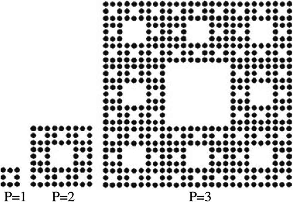
The generating sub array (P = 1) in this case has uniformly excited (where all elements are on) and uniformly spaced (uniform spacing of d = λ/2) 3 × 3 planar array of isotropic sources, with the center element turned off or removed. The array factor for this generating array may be expressed in the normalized form as [Reference Werner, Haupt and Werner179]

where,
ψ x = π[sinθcosϕ − sinθ 0cosφ0] (6)

here, θ0 and φ0 represent the main beam steering angles. Choosing an expansion factor of δ = 3 leads to the following expression for SC array factor for stage P.

Here the element count for each recursive stage of growth P is NP = 8P and in fact the arrays become significantly large at higher order stages. Using the above array factor expression, normalized array factor plots for various stages of the SC array are shown in Fig. 33. Due to the nature of the fractal algorithm, the array factor at n th stage is produced by the multiplication of all the factors of previous stages with the array factor of the n th stage. This procedure sucessfully leads to the rapid growth of array size as well as the population of elements along with quick increment of the gain. It is seen that, due to the nature of exhibition of fractal shape, the array factor at n th stage is produced by the multiplication of all the factors of previous stages with the array factor of the n th stage [Reference Werner, Haupt and Werner179].
Normalized far-field radiation patterns for (a) stage-2, (b) stage-3, and (c) stage-4 Sierpinski carpet fractal array using array factor expression as in (3) [Reference Karmakar, Ghatak, Mishra and Poddar180].

The array factor of conventional SC array has been considered [Reference Werner, Haupt and Werner179] with uniform interelement spacing of λ/2 and uniform amplitude excitations for the elements which are on. This limitation puts a barrier to this fractal array factor from the application of evolutionary techniques. Also the grating lobe maxima that inevitably occurs from the gradual increase of inter-element spacing of the array elements during the process of fractal development, should be suppressed and side by side the complexity of array factor calculations in at higher stages should be simplified.
In [Reference Karmakar, Ghatak, Mishra and Poddar180], an enhancement of theoritical foundations of fractal arrays like SC is presented. This optimization is based on SCF array, where the proposed iterative matrix will reduce the usual complexity [Reference Werner, Haupt and Werner179] for calculating the array factor of SC array at different stages of growth and also make the array factor suitable for the application of any evolutionary optimization techniques.
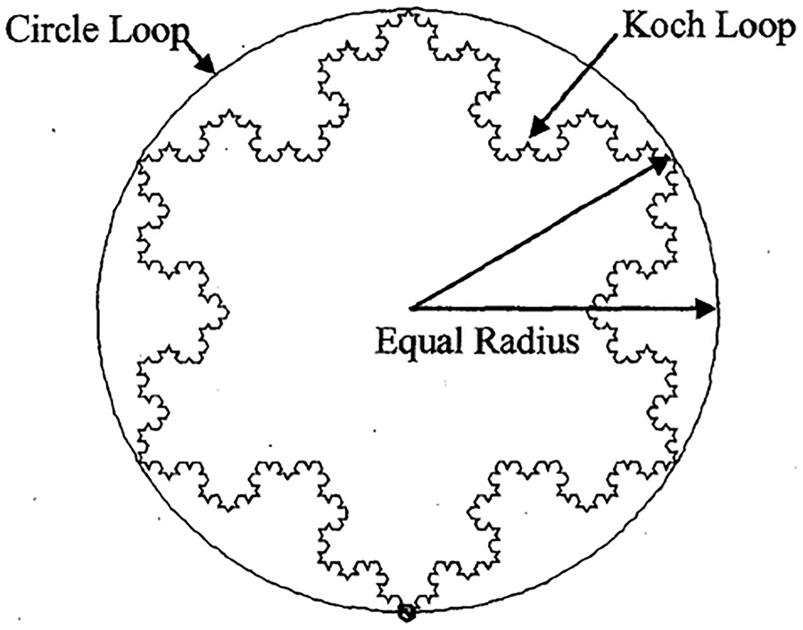
For planar fractal-tree arrays, a 2-D cellular automata is used in [Reference Sinha, Srivastava and Mehta181]. Different properties of atomic fractal arrays like multi-band behavior, low side lobe level, thinning are reported in [Reference Kravchenko182]. Miniaturization of wire and patch antennas using fractals has been shown in [Reference Gianvittorio and Rahmat–Samii183]. It is shown that, fractal patch array antenna significantly reduces mutual coupling between antenna elements. It is also shown that fractal designs can increase the input impedance of a small loop. The input resistance of a circular loop with a perimeter of 0.26 λ is 1.17 Ώ rather after the fourth iteration of Koch island curve with a perimeter of 0.68 λ, the structure has an input resistance of 26.7 Ώ (Fig. 34).
Loop antenna [Reference Gianvittorio and Rahmat–Samii183].
In [Reference Zygiridis, Kantartzis, Yioultsis and Tsibkoukis184], two popular methods are presented for efficient modeling of fractal antenna array structures. A new methodology has been introduced in [Reference Werner, Baldacci and Werner185] for exploiting the self-similarity as well as the symmetry of fractal-based arrays for the development of fast algorithms toward the calculation of impedance matrix and driving point impedance. Werner et al. introduced a fractile array in [Reference Werner, Kuhirun and Werner186] as a class of deterministic arrays that exhibit no grating lobes even when the spacing between the array elements is one wavelength. Some rare examples of such arrays are Peano–Gosper, terdragon, 6-terdragon, and fudge flake arrays. As an example, six-stage tetrahedron fractile array and the array factor plot are shown in Fig. 35.
(a) Sixth stage tetrahedron fractile array. (b) Corresponding array factor plot [Reference Werner, Kuhirun and Werner186].

It is found that neural networks [Reference Patnaik, Anagnostou, Christodolou and Lyke187] are an alternate approach in order to avoid the computational complexities of reconfigurable antennas. A new type of fractal-based design process has been presented that applies a robust genetic algorithm technique to evolve optimal array layouts based on polyfractal geometries [Reference Petko and Werner188]. Polyfractal arrays (Fig. 36) are a subset of fractal-random arrays that perform similarly; however, they are more responsive to large-scale genetic algorithm optimization.
(a) Illustration of the rapid recursive beam forming algorithm for a two generator polyfractal array. (b) Radiation pattern and element layout of a 178-element genetically optimized polyfractal array [Reference Petko and Werner188].

Optimization benefit from polyfractal array geometries can be obtained because these arrays can be described by fewer parameters than fractal-random arrays as well as possess recursive properties which can be used for rapid beam forming algorithms. Also, the unique structure of polyfractal arrays lends itself to more general variations of the crossover and mutation operators used in the optimization of genetic algorithm. One of these specialized mutation operators, called generator autopolyploidization, can be used to stimulate the evolution process when the optimization stagnates and appears to reach premature convergence. This offers polyfractal-based genetic algorithms an efficient path to complex design solutions, by first optimizing simple designs very quickly and then adding the increasing levels of complexity only when they are finally needed. For a given number of radiating elements and beam width in the broadside direction, Cantor-based ring-thinned arrays [Reference Hebib, Raveu and Aubert189] are presented (Fig. 37) for lower peak side-lobe level than one of the classical ring arrays composed of concentric rings with equal spacing between the rings. Moreover, in terms of beam width and peak side-lobe level, Cantor spiral arrays present the same performances than Cantor-based ring arrays with the alignment of radiating elements, but with a significant reduction of 10% in the number of elements.
(a) Symmetric Polyadic Cantor set at stage of growth at S = 1,2,3,4 and resulting concentric ring at stage 4. (b) Normalized array factor of the cantor-based ring array (N = 1, γ = 0.4367, a = 56.23λ, and S = 4) [Reference Hebib, Raveu and Aubert189].

In [Reference Yousefzadeh, Ghobadi and Kamyab190], a new microstrip patch antenna array is proposed with fractal patches instead of conventional rectangular patches in fractal configuration. It is seen that the mutual coupling between the antenna elements decreases substantially and also the input return loss decreases compared to the rectangular patch array. Another work presented in [Reference Petko and Werner191] expands on polyfractal array design methodologies by applying a robust Pareto optimization technique with the goal of reducing the peak side lobe levels at several frequencies specified over a wide operating bandwidth. A recursive beam forming algorithm and an autopolyploidy-based mutation native to polyfractal geometries are used to dramatically accelerate the genetic algorithm optimization process. This work also demonstrates that the properties of polyfractal arrays can be exploited to create designs with minimized grating lobes and relatively low side lobe levels over ultrawide bandwidths. A switched-beam antenna with reduced size and broadside beam based on the fractal Butler feeding network and fractal patch antenna array is presented in [Reference Chen, Wang and Zhang192]. The circuit sizes of the fractal-shaped branch-line couplers, 0 dB crossovers, and patch antennas are 43.7, 50.1, and 74% smaller than their conventional counterparts, respectively. A four-beam prototype has been constructed. Measurement indicates that broadside beams with side lobes below −10 dB are achieved. In [Reference Petko and Werner193], a novel nature-inspired design process has been proposed with specially formulated genetic algorithm technique to evolve optimal polyfractal array geometries. Customized routines for the genetic algorithm have been introduced that embody and utilize the unique geometry of the polyfractal array. In addition, the self-similar characteristics of the polyfractal array have been exploited to create a recursive beam forming algorithm, making faster array factor calculations which dramatically reduces the time required for the genetic algorithm to converge. Based on perturbed Peano–Gosper array geometries, an effective design technique for generating modular, wideband phased arrays (Fig. 38) has been introduced in [Reference Spence, Werner and Carvajal194].
(a) Example of a stage-1 generating array with perturbed element locations. The solid line denotes the PG curve and the dashed line denotes the initiator curve. (b) Stage-2 and (c) stage-3 arrays. (d) Geometry of a stage-3 Peano–Gosper array and with a contour plot of its normalized radiation pattern [Reference Spence, Werner and Carvajal194].

Unlike conventional perturbation techniques with independent adjustment of position of every element in an array, this technique is based on perturbing only six element locations along a stage-1 Peano–Gosper generator curve and then using these locations to iteratively construct larger arrays which allows for a tractable perturbation process that is easily combined with any optimization techniques. Hybrid fractal direct radiating arrays with high-performance features and suitable for satellite applications are synthesized in [Reference Siakavara195]. The main advantage of the proposed arrays is the very small number of elements and driving points which leads to a feeding network of low-cost and complexity. It has been shown that nature-inspired array design methodologies can provide solutions that exhibit these ultra-wideband characteristics. In [Reference Gregory, Petko, Spence and Werner196], the article provides an overview of two such designs: linear polyfractal arrays and planar arrays of aperiodic tilting's. Robust nature-inspired genetic-algorithm optimization techniques were utilized in this design of both types of arrays in order to achieve the best-possible UWB performance. It is shown that arrays based on Gosper curves possess several attractive properties including broadband capabilities, low sidelobes, uniform amplitude excitations, the ability to use recursive pattern formulations, and modular sub array architectures. They also offer a range of array sizes and modular configurations that are not inherent to conventional Peano–Gosper arrays. It is seen that generalized Gosper space-filling curves [Reference Spence and Werner197] can be suitabel to a variety of electromagnetics and antenna applications. Arrays based on these curves possess several attractive properties which include broadband capabilities, low sidelobes, uniform amplitude excitations, the ability to use recursive pattern formulations as well as modular sub-array architectures and also offers modular configurations which are not inherent to conventional Peano–Gosper arrays.
A novel multi-band antenna [Reference Kuzu and Akcam198] is designed and manufactured by combining a fractal shape and DGS achieving superior performances yet within a compact architecture which makes this design suitable for geostationary satellite communications (Fig. 39). In this structure, Apollonius circles are utilized in order to design a sui generis fractal shape which was etched on the ground face of the antenna to tune different frequency bands. Finally, the designed antenna elements are aligned to build 2 × 2 array antenna structure. In [Reference El-Khamy, Eltrass and El-Sayed199], a new antenna array is designed to to combine multi-band [Reference Sanchez200] features of thinned fractal antenna arrays with the adaptive beam forming requirements. In [Reference Alibakhshikenari, Virdee, See, Abd-Alhameed, Ali, Falcone and Limiti201], a decoupling metamaterial (MTM) configuration based on fractal EMBG structure is presented to enhance the isolation between transmitting and receiving antenna elements in a closely packed patch antenna array.
Antenna array dimension. (a) Side view. (b) Front view [Dimensions are in 'mm'] [Reference Kuzu and Akcam198].

This section focused on the design aspects of fractal arrays and the optimization techniques which are one of the key tools for the enchantment of fractal antenna array behavior. In this manner, various optimization techniques have been applied by various researchers to improve array factor properties as well as to reduce the antenna elements at larger iteration levels. Still there is good scope to do a wider research work in this combination.
Conclusion
Fractal geometry has many applications in life and opened up innovative research directions in almost all branches of science and engineering gaining from the new insights it has provided. The primary focus of this review article is to summarize the developments in the field of fractal antenna engineering with basic discussions and examples. It is not possible to cite every published work on fractals still It has covered more than 200 articles that provides basic performance properties of various types of fractal antennas and arrays which has a wide range of applications. The review article reveals that fractal loop and dipole wire radiators are contrasted with linear loop and dipole antennas leading to miniaturization. When revisiting wideband antennas based on fractal, it is seen that in comparison to Euclidian UWB antennas, fractal UWB antennas possess not only small size, light weight, and thin shape for portable devices that have a rigorous limitation of space, but also wide bandwidth and good radiation characteristics with lower cross polar level. It is also seen that the concept of fractal can be applied to the design and analysis of arrays by either analyzing the array using fractal theory or by placing elements in fractal arrangement. Needless to say that the ideas of fractal geometry have been in existence for a long time but the emerging interest in fractal antennas has essentially ridden on the back of advances in computer development. In last word, the author apologize to researcher community if any novel contribution in this domain is skipped unknowingly and unintentionaly during this review process.
 Anirban Karmakar has received Ph.D. in Engineering from Jadavpur University, Kolkata, India, in 2015. He has more than 13 years of teaching experience and is currently holding the post of Assistant Professor in the Department of Electronics & Communication Engineering at Tripura University (A Central University), India. He has almost 40 research articles in refereed journals and international conference proceedings. He has served as a reviewer in different international journals. He was awarded the best paper award from different international conferences. He is a Senior Member of IEEE and has organized different workshops in the capacity of a convener and completed various funded projects received from UGC. Currently four research scholars are pursuing Ph.D. under his guidance. His areas of interest include planar and fractal wideband antennas, arrays, circular polarized antennas, DRA, etc.