Fertility rates in most of the developed world are at historical lows, the result of decades of steadily declining fertility. For the United States, replacement-level fertility is the culmination of a demographic transition more than 200 years in the making.Footnote 1 Economists have put forward a number of theories to explain this demographic transition. Beginning with Gary S. Becker (Reference Becker1960), many have conceptualized fertility as the outcome of a household's utility maximization problem subject to its resource constraints. In Becker's formulation, children are inputs into the household's production, and the household's fertility decision incorporates not only the costs of bearing and rearing children, but also the positive returns associated with the child's household production. The driver of fertility choice is the price of children. Increases in costs or reductions in benefits imply a commensurate increase in child prices and a reduction in the household's demand for the same. Becker's formulation and its derivatives, collectively “demand theories” of fertility, have given rise to a host of economic theories specific to the U.S. fertility decline highlighting ways in which child prices have increased over time.Footnote 2
A simple use of demand theories to explain U.S. fertility patterns is as follows: Early in the nineteenth century, child prices were low. Children worked as laborers on the family farm until early adulthood before marrying and moving, generally to a nearby location. Once the child left the homestead, the child still contributed positive value to parents by serving as old-age security, a critical service in the absence of a mature financial system. Over the course of the nineteenth and twentieth centuries, however, the price of children began to rise. Higher education costs and rising opportunity costs of female time spent in childrearing increased the costs associated with children, and increased migration, an occupational shift from agriculture to manufacturing and service sectors, more stringent child labor laws, an increasing availability of substitute old-age insurance, and downward pressure on manufacturing wages reduced their benefit. The result was a reduction in demand for children and, thus, a lower fertility rate.Footnote 3
To assess whether changes in child prices were instrumental in determining fertility rates early in the U.S. transition, it would be useful to observe a “shock” that changes the price of own children for households yet is independent of other characteristics of the household. I propose that southern slaveowners in the nineteenth century were subject to exogenous shocks to the prices of their children via the fertility of their slaves. (Note that “child prices” in this paper refer to the inherently unobservable prices of the slaveowner's own children. This concept is distinct from prices of slave children traded on the market.) Substitutability between own children and slave children implies that positive shocks to slave fertility would have reduced the productivity of the slaveowner's own children and resulted in lower fertility rates for slaveowners. For simplicity here, and throughout the paper, “slave children” are those born to female slaves and “own children” are those born to a female slaveowner or the male slaveowner's wife, regardless of paternity.
I construct a panel dataset of slaveowners’ household characteristics and slaveholdings and use this to measure the fertility response of owners to slave births. I find that white slaveowner fertility was negatively correlated with slave fertility in the years prior, conditional on both year and household fixed effects in white fertility; the result is both economically and statistically significant. These correlations are stronger on farms with fewer slaves and in states where slave exports were low and are robust to tests related to measurement error in slave fertility.
The fertility of owned slaves was not always independent of the preferences of the slaveownerand may have been otherwise correlated with unobservables of the household also impacting white fertility. I utilize slave emancipation in 1865— an event unaffected by the preferences of slaveowners and orthogonal to household characteristics—as an additional test of demand theories of fertility. Again, the labor shock resulting from emancipation changed the productivity potential of the former slaveowner's own children and, thus, child prices. Using panel data to measure the relationship between pre-emancipation slaveholdings and post-emancipation fertility, I find that slaveowning households for whom the price of children decreased the most after emancipation experienced the highest subsequent fertility rates.
Thus, estimates of fertility behavior following both slave fertility events and the 1865 emancipation of southern slaves indicate that child prices and household fertility were negatively correlated in the mid-nineteenth century U.S. South. These findings are consistent with demand theories of fertility decline early in the U.S. demographic transition.
CONCEPTUAL FRAMEWORK
Consider an antebellum slaveowning household whose production inputs, in addition to capital, consist of white family members plus the household's slaves. The household chooses inputs to maximize lifetime utility subject to a budget constraint. Child prices incorporate direct and indirect costs the household incurs in bearing and rearing the child less the benefits the child brings to the household including the present value of their future contributions to household production. A fully specified model consistent with this intuition is contained in the Online Appendix.Footnote 4
Now consider the effect of a slave birth on the price of the slaveowner's own child. In a simple model of household production, slave children and own children are substitutes in a production function with diminishing marginal returns. An exogenous increase in the number of slave children results in a reduction in the benefit coming from the owner's own children and an increase in their price. In this model of fertility decision-making, own fertility of the slaveowner will fall in response.Footnote 5
The same dynamic exists in other models of fertility behavior. In particular, Susan B. Carter, Roger L. Ransom, and Richard Sutch (Reference Carter, Ransom, Sutch, Guinnane, Sundstrom and Whatley2003) put forth a life cycle savings model where children are a viable means for the household to save for future needs. In the absence of more formal instruments to save for the needs of old age, households welcomed the birth of own children as a way of ensuring they would be cared for in later years. The absence of primogeniture laws in the United States implied that children might eventually “compete” for the right to inherit the household's land and, in exchange, would be relied upon to care for parents in their old age. If slave children were alternative solutions to the intertemporal savings problem, then an exogenous change in their number represented a shock to the household savings rate and reduced the incentive of slave owners to save via their own fertility.Footnote 6 Again, increases in the number of owned slaves result in rising prices of the owner's own children.
This singular prediction for household behavior can be augmented to exploit differences in the production substitutability between slave children and own children across households. Production substitutability was strongest on farms where the owner's family members and slaves worked side-by-side and performed similar functions. Because slaveholding size was positively correlated with labor-specialization practices separating family members from slaves (Steckel Reference Steckel, Gaspar and Hine1996; McCurry Reference McCurry1995; Hahn Reference Hahn2006), the smaller the number of slaves in the household, the stronger the production substitutability.Footnote 7 Thus, the magnitude of an owner's fertility response should be negatively correlated with the size of holdings; owners of smaller slave labor forces should be more sensitive to slave fertility on their farms.
Slave emancipation in 1865 provides additional predictions for household fertility behavior. Emancipation represented a positive shock to the price of non-family labor in the postbellum South for two reasons. First, emancipation brought a reduction in the efficiency of former slave labor both because the efficiency of larger farms and plantations was replaced by small plot farming and sharecropping and because the labor available for hire in the postwar labor market was negatively selected in terms of efficiency (Moen Reference Moen, Fogel and Engerman1992; Ransom and Sutch Reference Ransom and Sutch2001). As a result, the productivity of Southern labor declined by approximately 30–40 percent between 1860 and 1880 (Fogel and Engerman Reference Fogel and Engerman1974) and, for a given number of labor hours in the market, the productivity of those hours declined. Only if hourly wages fully adjusted to reflect the reductions in productivity would the (effective) cost of labor not change (Margo Reference Margo, Eltis, Lewis and Sokoloff2004). Second, former slaves participated in the labor market at a lower rate than they had under coercion. As a result, emancipation represented a negative supply shock, and the price of labor increased accordingly (Ransom and Sutch Reference Ransom and Sutch2001). Importantly, Fogel and Engerman (Reference Fogel and Engerman1974) conclude that Southern households did not anticipate emancipation, at least on a large scale, in 1860 when slave ownership is measured in my data; slave prices did not begin to decline in reflection of the emancipation risk until 1861 (Fogel and Engerman Reference Fogel and Engerman1976).
Unlike the effects of slave fertility, the direction of the shock to the price of the slaveowner's own children resulting from emancipation is ambiguous and depends on whether own children and slaves were substitutes or complements in household production. As discussed above, slave children were highly substitutable for own children on farms with small numbers of slaves in the pre-emancipation years. Because the post-war method of farming on a small farm closely resembled the pre-war method, a continued need for family labor ensured a high marginal product for own children after 1865 and comparatively low child prices.
On the other hand, larger farms with more substantial pre-war slave holdings resorted, at least partially, to sharecropping, and the impact of slave emancipation on the marginal product of own children is not clear. At the same time, there was likely a strong pre-emancipation complementarity between adult slaves and the slaveowner's children in households with larger numbers of slaves. In the pre-war period, these slaveowners had the added luxury of employing female slaves as house servants, a job which included tending to the owner's own children (Olson Reference Olson, Fogel and Engerman1992).Footnote 8 As a result, own children and adult slaves may have been complements in production on these farms as adult slaves, particularly females, enabled the production of children. Emancipation then raised the costs associated with the slaveowner's own children and increased own child prices.
The emancipation experiment thereby generates two testable implications for slaveowner fertility behavior under demand theories of fertility. The lost labor of slave children should have raised the marginal product of labor for own children and raised white fertility in households with small pre-war slave holdings. But the loss of slave adults, especially adult females, to emancipation may have raised the rearing cost of own children and lowered white fertility in slaveowning households with larger pre-war slave holdings.Footnote 9
Caveats to the empirical strategy highlighted above emerge when one considers other differences across farms that may have been correlated with the size of the pre-war slave labor force but would also have affected household fertility. Possible confounders include, but are not limited to, infant-and-child mortality, and slave breeding and trade. I examine each of these confounders later in the paper. In the Online Appendix, I consider the implications of endogenous slave fertility and white paternity, increasing returns in Southern agriculture, and differences in productivity by crop mix. In each case, the results are somewhat sensitive to these confounders, but the paper's main conclusions remain.
DATA
The data for this project link southern households between manuscripts of the 1860 and 1870 U.S. Census of Population schedules and the 1860 U.S. Census of Slave Inhabitants. A 5 percent random sample of slaveowners from the 1860 Census of Slave Inhabitants and their complete slaveholdings is available from Ruggles et al.(Reference Ruggles, Sobek, Alexander, Fitch, Goeken, Hall, King and Ronnander2008). For each slave, his or her age, sex, and race (black or mulatto), in addition to the owner's name and geographic location, are available. I limited this sample to include only rural slaveowners from six states of the Deep South (Alabama, Florida, Georgia, South Carolina, Mississippi, and Texas) and those who owned their slaves individually, excluding slave-owning corporations and partnerships.
This generated an initial sample of 6,974 slaveowners (holding 89,870 slaves) in 1860. The slave schedules contain no demographic characteristics of slaveowners; instead, each slaveowner was matched to the manuscripts of the 1860 Census of Population based on their full name and geographic location. Ninety-two percent of slaveowners were successfully matched to their population schedule enumeration.Footnote 10 I restricted the sample to married couples with female spouses in the fertile age range (35 or younger) because marital fertility is the outcome of interest.Footnote 11 The cutoff age of 35 was chosen to ensure that the female would remain fertile for at least five years following emancipation (through 1870).Footnote 12
This linking process generated a sample of 2,491 households and the composition of their slave holdings in 1860. To capture post-emancipation outcomes, I linked slaveownersto the 1870 Census of Population schedules using information on the 1860 nuclear family (slaveowner, spouse, and own children). Match criteria included the name, age, and birth place of these family members, and 1,211 slaveowners were successfully located in the 1870 Census.Footnote 13 A linked sample of non-slaveowners was also generated as a control group for the analysis related to slave emancipation.Footnote 14 For all slaveowning families, two research assistants transcribed information from the 1860 and 1870 enumeration forms, recording the name, occupation, literacy, age, real estate wealth, and personal wealth of each member of the nuclear family.
One final adjustment to the dataset was required. For the purpose of determining marital fertility rates, slaveowners were removed from the sample due to death of a spouse, divorce, remarriage, and/or separation before the 1870 enumeration. The resulting base sample contains 1,199 slaveowning households, of whom 975 were slave owners.
The slaveowner's own fertility history is constructed based on the presence of children in the 1860 and 1870 manuscripts. For each household j in year t, F W jt measures the number of white children born to the house hold. For slaves, fertility histories are constructed using the 1860 slave schedules. For each household j in year t ∊ [1846, 1860], FS jt measures the number of slave children born in that household-year. For instance, an eight-year-old child observed among the slave labor force in 1860 is coded as an 1852 fertility event.
In both cases, fertility metrics will necessarily exclude births that ended in the death of a child prior to census enumeration or births for which the child was no longer living in the household. The biases imparted by mismeasurement are discussed following the empirical results.
SLAVEOWNER RESPONSES TO SLAVE FERTILITY
Average fertility rates per household-year are reported in Table 1. Households experienced slave births in one out of every three years, on average, and a white child birth occurred once every four years. Slave and white fertility both exhibit longitudinal variation. White fertility is highest in Texas and Mississippi; slave fertility is highest in South Carolina and Florida.
To test the implications derived above, an event study framework is used to measure the impact of slave fertility in a household on white fertility between 1850 and 1860. White fertility in the household in year  is the dependent variable which depends on the five-year history of slave births:
 in years t through t − 4. The model also includes year and household j fixed effects:

where t ∊ [1850, 1860] and relevant slave fertility events occurred between 1846 and 1860.Footnote 15 The γk coefficients represent the conditional change in fertility for households in year t following a slave fertility event in year t − k.
In addition to single-year effects identified in Equation 1A, I estimate the cumulative effects of slave fertility by modifying Equation 1A to capture two- and four-year cumulative slave fertility histories. When measuring the impact of the past two years of slave fertility, indicators for slave fertility in years t, t − 3, and t − 4 remain and the estimating equation becomes

where γ12 in Equation 1B represents the relationship between current-year white fertility and cumulative slave fertility over the past two years. For the model with four years of cumulative slave fertility, the estimating equation becomes

where γ1234 in Equation 1C represents the relationship between current-year white fertility and cumulative slave fertility over the past four years.
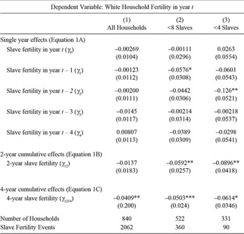
Results from estimating Equation 1A are located in the top panel of Table 2. Column 1 incorporates all households in the sample. For each slave born within the household, the results indicate a significant contemporaneous increase in white fertility of 0.017 children (from an average of 0.259), but no significant correlation between white fertility and slave fertility in any year prior. Similarly, the relationship between white fertility and cumulative slave fertility in the two years prior (γ12) identified in Equation 1B is small and statistically insignificant. The coefficient on slave fertility in the past four years (γ1234) from Equation 1C, on the other hand, is statistically significant; the point estimate of −0.038 children corresponds to a roughly 15 percent reduction in fertility.
Consistent with expectations regarding substitutability between slave and own children, the significant correlation between current year white fertility and slave fertility in the past four years in the full sample is driven by households with small numbers of slaves. Column 2 is limited to households owning fewer than eight slaves (62 percent of households), and white fertility is negatively correlated with slave fertility in each of the previous years, significantly so for a slave birth occurring one year prior. Estimated coefficients for slave fertility aggregated over the last two (γ12) and four (γ1234) years in the bottom panels of Table 2 indicate a reduction in household fertility of 0.054 to 0.057 children, or roughly 20 percent. At the same time, contemporaneous white fertility (γ0) is unaffected by slave fertility in the same year for these households.
Limiting the sample to households with the smallest slave labor forces, those who owned fewer than four slaves in 1860 (38 percent of households), estimates in Column 3 indicate even more substantial impacts on white fertility. In the year following a slave fertility event, white fertility is reduced by 0.081 children (30 percent) and in year 2 by a statistically significant 0.12 children (46 percent). Indeed, taken together, each slave birth in one of the last two years is associated with a white fertility reduction in these smallest households of 0.098 (41 percent). A slave birth in one of the past four years is associated with a reduction of 0.066 white children (28 percent).
The coefficients in Table 2 can be used to calculate a displacement rate— the number of white children displaced by a single slave birth within the household. Summing up the single-year estimates of for yk years 0–4, the displacement rate is 0.11 own children for households containing fewer than 8 slaves and 0.20 for those containing fewer than 4 slaves.
An obvious question is whether the fertility patterns documented in Columns 2 and 3 are simply a continuation of behavior prior to slave birth events. Although this does not fully explain the lagged timing, and although household fixed effects eliminate fixed differences in white fertility across households, perhaps slaveowners with smaller slave labor forces were also in low-fertility eras of their own fertility histories. Column 4 contains estimates from a falsification test whereby Equations 1A–1C are converted to measure the impact of slave fertility in years t + k on year t household fertility for households with fewer than eight slaves.Footnote 16 No coefficient on future slave fertility is significant. In estimates for cumulative future slave fertility, a two-year measure (covering years t + 1 and t + 2) has a statistically insignificant, although sizable, coefficient. The four-year effect (for years t + 1 through t + 4) is effectively zero.Footnote 17
Equations 1A–1C Estimation Results

*= Significant at the 10 percent level.
** = Significant at the 5 percent level.
Notes:
The table lists results from estimating Equation 1A, 1B, or 1C for slave fertility events between 1846 and 1860 (and household fertility responses from 1850 through 1860). Single year impacts are estimated using Equation 1A. Cumulative effects over two and four years are estimated using Equations 1B and 1C, respectively. All specifications also include household and year fixed effects. Column 1 includes all households in the sample. Column 2 includes only those households owning fewer than 8 slaves in 1860. Column 3 includes only those households owning fewer than 4 slaves in 1860. Column 4 contains the pre-trends for households owning fewer than 8 slaves such that γ k represents the impact of slave fertility in year t + k. Standard errors in parentheses.
Source:
Author's calculations from Census data described in text.
A final concern about the results in Table 2 is that the contemporaneous effect of a slave child birth (γ0) is positive, large and, for the full sample, marginally statistically significant. This result appears to be due entirely to “age-heaping,” the tendency of households to report ages of household members that end in 0 or 5. In particular, there is a substantial mass of both 5-year-old children and 5-year-old slaves in the 1860 census enumerations, especially among owners of larger slave labor forces, generating a spurious correlation between slave births and white births in the same year. Potential corrections for the age-heaping issue, explored in more detail in the Appendix, do not affect other conclusions from Table 2.
ROBUSTNESS CHECKS AND ADDITIONAL ANALYSIS
Table 2 results indicate some slaveowning households responded to slave fertility within the household with reduced white fertility, in accordance with demand theories of fertility. This section evaluates whether these results are robust to the confounding effects of infant-and-child mortality and of slave trading. I also present results separately for “exporting” and “importing” states based on the net flow of slaves in trade. Further robustness checks related to endogenous slave fertility, slave child paternity, and crop mix are contained in the Online Appendix.Footnote 18
The Role of Infant-and-Child Mortality
Both slave and white fertility variables are subject to one-sided measurement error resulting from mortality in the years prior to census enumeration. Infant mortality among slave children was higher than that for white children (Steckel Reference Steckel1986), but both populations experienced substantial losses in the first few years of life. If measurement error in white fertility is uncorrelated with observed slave fertility, the estimates in Table 2 are unbiased. This seems unlikely given that slave and white children were exposed to similar disease environments, nutrition opportunities, environmental stressors, etc.
Intuitively, if white children and slave children were subject to positively correlated infant mortality shocks, this generates spurious positive correlation in slave and white fertility as white fertility will appear to be high when observed slave fertility is high and low when observed slave fertility is low. Estimates in Table 2, which indicate a negative correlation between slave and white fertility, can then be viewed as an upper bound on the true relationship.Footnote 19
Bias Due to Slave Trades
In addition to infant-and-child mortality, the trading of young slaves imparts measurement error in slave fertility. The market for child slaves sold alone (without an accompanying mother) was quite small, but the market for slave children sold with a parent was more substantial.Footnote 20 If trading propensity increased with the number of owned slaves, the resulting measurement error in slave fertility is correlated with the size of the slave labor force and may contribute to the lower correlation between slave fertility and household fertility therein.
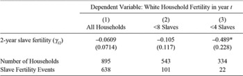
To investigate this possibility, the panel data are limited to slave birth events occurring in 1857–59 as the very youngest slaves were least likely to be sold. White fertility responses to slave births in the previous two years (γ12 from Equation 1B) are then estimated using white fertility measured in 1859 and 1860. Resulting estimates, located in Table 3, are far less precise relative to the baseline specifications, reflecting the shorter time series of observations. But the general pattern remains— households with smaller numbers of slaves responded more strongly to slave fertility than did those with larger slaveholdings.
As an additional test of the importance of slave trading for the results in Table 2, I estimate the amount of mismeasurement necessary to generate the results in Table 2 if the true coefficients are equivalent across subsamples represented by Columns 1 and 3. To do so, I generate random mismeasurement in slave fertility for households with fewer than four slaves (Column 3) until the estimated white fertility response to two years of slave births (γ12) is the same as for the full sample in Column 1. Results indicate that roughly 50 percent of household-year slave fertility observations would need to be mismeasured for this subsample to generate a point estimate for γ12 equivalent to that in Column 1 of Table 2. This amount of mismeasurement in slave fertility for the full sample is highly unlikely given estimates of the volume of trade for young children. Estimates from Sutch (Reference Sutch, Engerman and Genovese1975) indicate that approximately 8 percent of slave children under the age of ten entered the interstate trade between 1850 and 1860. Bancroft (1931) estimates that the intrastate trade was 50 percent as great as interstate movements, resulting in a total churn for young slave children of approximately 12 percent, far lower than the 50 percent required to equalize estimates of γ12 across columns.
Results in Slave Exporting States
The literature on slave breeding and trade suggests that in locations where slave agriculture was relatively less profitable, slaves were assets not because of their production potential on the household's own farm, but because they could be sold to areas with more productive agricultural systems. The direction of trade was from east to west with states on the northern and eastern edges of the slave South (District of Columbia, Virginia, Maryland, Kentucky, Delaware, Tennessee, North Carolina, South Carolina, and Georgia) exporting those slaves to the importing states of Texas, Arkansas, Florida, Louisiana, Mississippi, Alabama, and Missouri (Sutch Reference Sutch, Engerman and Genovese1975).
Equation 1B Estimation Results for Slave Births in 1857–58

* = Significant at the 10 percent level.
Notes:
See Notes for Table 2. Results reflect household responses (measured in 1859–1860) to slave fertility in 1857–1858. Standard errors are contained in parentheses.
Source:
Author's calculations from Census data described in text.
A household's intent to sell slaves would substantially reduce the substitutability of slave and white children in the production function as the slaveowner's own children would not have been substitutable for slave children in the market for slaves. The responsiveness of free whites to slave fertility should then be reduced in states where the intent to sell was higher.
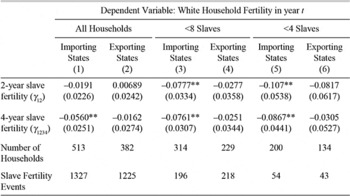
I bifurcate the sample into exporting and importing states to evaluate this additional prediction. Georgia and South Carolina were net slave exporters in this period, but neither were very large exporters. In South Carolina, 13.4 percent of slaves were sold west and in Georgia the rate was 2.4 percent. (This compares to a net export rate of 32.6 percent in Delaware.) Approximately 10 percent of those exported from South Carolina were under age 10, and the percentage in Georgia was lower still.Footnote 21
The odd-numbered columns of Table 4 contain estimated coefficients for γ12 from Equation 1B and for γ1234 from Equation 1C for importing states alone and even-numbered columns measure the same for exporting states. There is a clear pattern of stronger fertility responses in importing states, consistent with greater substitution in those states. For households with fewer than eight slaves (Columns 3 and 4 of Table 4) in South Carolina and Georgia, the white fertility reduction in response to a slave birth in the two years prior is 0.028 compared to 0.078 elsewhere across the South. For the four-year horizon, exporting states showed a white fertility reduction of 0.025, with the comparable number again being three times as great, 0.076, across the rest of the South. For households with fewer than four slaves (Columns 5 and 6 of Table 4), correlations between slave births in the last two or four years and white fertility are again more pronounced in importing states, although the differences are not as exaggerated. A similar exercise comparing fertility in Texas and Mississippi with the remaining states (not shown) indicates a slightly more negative relationship between slave and white household fertility in the border states, but the difference is not substantial.
Equations 1B and 1C Estimation Results for Importing and Exporting States

* = Significant at the 10 percent level.
** = Significant at the 5 percent level.
Notes:
See Notes for Table 2. Exporting states columns (2, 4, and 6) include households residing in South Carolina and Georgia only. The remainder of the sample households are in importing states. Standard errors are contained in parentheses.
Source:
Author's calculations from Census data described in text.
These results indicate that states where slave children were least likely to contribute to household production in the future (including at old age of the slaveowners), slaveowners exhibited weaker responses to slave fertility, consistent with a lower substitutability between own and slave children in these locations. The muted fertility response is apparent across all sizes of farms, although it is least pronounced on the smallest farms.
SLAVEOWNER RESPONSES TO SLAVE EMANCIPATION
The conclusions in the previous section must be qualified by the acknowledgement that slave fertility was in no sense randomly assigned to households. Slaveowners influenced the fertility of their slaves in a number of ways, some more coercive than others. In addition, if low-fertility households were more likely to select high-fertility slaves, the results in Table 2 may partially reflect that selection.Footnote 22 Although it seems unlikely that endogeneity of slave fertility and/or selection would generate the specific pattern of no correlation in year t followed by reduced white fertility in years t + 1 and following, these concerns motivate using slave emancipation as a second shock to own child prices. The conceptual framework indicates that the substitutability between slave and own children was highest for owners of small numbers of slaves while complementarities between adult slaves, particularly females, and own children were highest for owners of large numbers of slaves. Implications from demand theories of fertility, then, are that post-emancipation white fertility will be highest for owners of small slave labor forces containing young children and lowest for owners of large slave holdings with adult female slaves.
The dependent variable of interest is the household's post-emancipation fertility between 1866 and 1870 (F W i,1866-1870)—the number of children in the household in the 1870 Census of Population whose reported age was 0–4 years. This is the five-year span immediately following emancipation and the end of hostilities in the Civil War and was chosen to limit biasing results with a “war effect” that differed by household. As Confederate forces surrendered at Appomattox, Virginia in April 1865, 1866 was chosen as the beginning of the fertility window.
Some fertility in this period may reflect catch up fertility lost during the war. Because larger slaveowners were less likely to fight in the Civil War due to the “20-Negro Rule” exempting them from service, we might expect a bigger catch-up effect among the smallest slaveowners. But there is little reason to think this catch-up behavior would have been affected by the gender and age composition of 1860 slaveholdings, conditional on the size of the overall slave labor force.
Equation 2 is estimated for each household residing in i county c in the sample in 1870:

where P i,1866–1870 is the price of the slaveowner's own children and is proxied by a vector of characteristics describing the household's slaveholdings in 1860. Indicators are used for the size of the slave labor force in 1860 (1–3, 4–7, 8 or more slaves), its age composition (0–2, 3–6, 7–10, 11–15, 16–35, 36 or more years of age), gender, and interactions among these categories. County-level fixed effects, vc , are included to absorb fertility differences resulting from idiosyncratic county-level variation.Footnote 23 Means of white fertility and slaveholding variables used to proxy P i,1866–1870 are located in Table 5.
Additional controls in X i,1866–1870 include the ages and squared ages of the slaveowner and his/her spouse, an indicator for whether the male household head is employed in agriculture, numeracy as a proxy for education, the household's 1870 real estate and personal wealth, and the change in the household's real estate and personal wealth levels, separately, between 1860 and 1870.Footnote 24 Fixed effects for the male head's place of birth are included to capture variations in fertility related to cultural and religious norms. Finally, in an attempt to account for any fixed effects in fertility (differing tastes, etc.) and also the possibility that families pursued a “target” family size, the household's fertility between 1856 and 1860 is also included as a component of X.Footnote 25
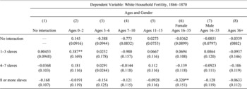
Table 6 contains estimated coefficients for Equation 2 under a variety of proxies for white child prices.Footnote 26 The sample mean white fertility rate is 1.04 (Table 5), and coefficients can be roughly interpreted as percentages. As a first step, P i,1866–1870 includes indicators for slaveholding size only, and coefficient estimates are located in the “No interaction” column (Column 1). Throughout the table, non-slaveowners are the omitted category. I then control for age/gender variables only (“Ages 0–2” through “Ages 36+”), interacting gender with age for adults aged 16–35.Footnote 27 Estimated coefficients for each category indicator are reported in the “No interaction” row.
Summary Statistics—panel Data on Household Fertility and Slaveholdings, 1860–1870 for Table 6

Source:
See text.
These initial results indicate no statistically significant relationship between the composition of a household's 1860 slave holdings and the household's white fertility rate after 1865. But the testable implications from the conceptual framework indicate important interactions between these categories. For each age/gender category listed in Table 5, Equation 2 is estimated with an interaction term between that age/gender indicator and the three size indicators, leaving the remaining age/gender indicators without interaction. For example, estimates in the bottom three rows of Column 2 represent the conditional difference in white fertility between 1866 and 1870 for a household that owned slaves aged 0–2 and owned between 1 and 3 slaves, between 4 and 7 slaves, and 8 or more slaves in 1860, respectively, relative to their non-slaveowning peers. This exercise is repeated for every age and gender category.
Equation 2 Estimation Results

** = Significant at the 5 percent level.
Notes:
The table reports the estimated marginal effects on average household fertility under a variety of proxies for Vi in Equation 2. The “No Interaction” rows and columns represent the impact of indicator variables for size of holdings and age/gender categories, uninteracted. Each column, 2–8, gives the coefficients for a model including all age/gender categories with interactions with size of holdings for the column specified. For example, Column 2 contains a vector of indicator variables in Vi including all age/gender categories along with interaction terms between the 0–2 age category and each of the three size of holdings categories. Sample size is 1,199. Standard errors are in parentheses.
Source:
Author's calculations from Census data described in text.
Incorporating interaction terms between size and age/gender dimensions in Equation 2 exposes substantial differences in fertility outcomes across groups. In Column 2, the post-1865 fertility of owners with the youngest slaves (aged 0–2 in 1860) decreases with overall size of slave holdings. Conditional on the controls in X, owners of a slave child and one to three slaves overall have 0.387 more own children per household than non-owners following emancipation while those owning between four and seven slaves have 0.181 more own children per household, although this latter result is not statistically significant. Slaveowners with large slave holdings containing young children, on the other hand, exhibit no notable fertility difference relative to non-owners after 1865. For former owners of slaves aged three to six, the same general pattern holds (Column 3); the owners of the smallest slave labor forces have higher post-emancipation fertility than owners of the largest forces and the owners of four to seven slaves lie somewhere in between, although the results are not statistically significant. Estimated coefficients on the size of slaveholding interaction terms for owners of slaves aged seven to ten (Column 4) and eleven to fifteen (Column 5) are insignificant.
For owners of slaves aged 16 to 35, post-emancipation fertility decreases with the size of slaveholdings, and the estimated coefficients for the largest size category are negative and statistically significant (not shown). This result is driven entirely by the behavior of owners of female slaves in this age category (Column 6) where owners with the largest number of slaves in 1860 have a statistically significant 0.320 fewer own children after 1865 than their non-slaveowning peers. Estimated coefficients for the interaction between adult females and the other size categories are insignificant but follow the expected pattern; fertility reductions are larger for owners of medium-sized slave labor forces than for owners of one to three slaves. Owners of male slaves in this age category exhibit a weaker gradient along the size of slaveholdings dimension (Column 7), and the estimated coefficients on the interaction terms are not statistically significant. Estimated coefficients on the interaction between the oldest age category (36 and older) and the size categories are not significant (Column 8). A similar gender stratification for the age 36 and higher category (not shown) produces similarly insignificant results.
As a robustness check (not shown), I limit the sample to females aged 30 years and younger in 1860. The estimated impacts on fertility in Table 6 are stronger for this group, consistent with the notion that they were more fertile in the post-1865 years. In addition, a replication of Table 6 for above- and below-median cotton production counties (located in the Online Appendix) indicates that the positive post-emancipation fertility response of owners with young slave children and small holdings is substantially more pronounced in above-median cotton counties. At the same time, the reduction in fertility associated with the loss of an adult female slave is also greater in relatively low-cotton locales, perhaps reflecting the fact that female slaves on cotton plantations were more likely to be field slaves than house slaves and thus exhibited a lower complementarity to the slaveowner's own children.
CONCLUSION
The number of children born to slaveowners in this sample is negatively correlated with proxies for child prices, consistent with demand theories of fertility behavior emphasizing household optimization given the price of potential offspring. In the pre-emancipation era, the birth of a slave child, and presumed reduction in the marginal product of white children, is associated with reduced white fertility in households with small numbers of slaves. In the post-emancipation era, households with small slave labor forces and young slave children in 1860 bear significantly more white children after 1865, consistent with reduced own child prices for former slaveowners in the post-emancipation years. Households with large pre-emancipation slave holdings containing adult female slaves, who may have been complementary to child production, exhibit significantly lower white fertility after 1865.
At the aggregate level, reductions in southern white fertility are not apparent until the end of the nineteenth century while reductions in nationwide rates are evident by 1800. Innovation and diffusion theories of fertility decline explain the southern delay as a result of the slow diffusion of social norms and technologies related to fertility control. In support of these theories, fertility control is apparent earliest in the Northeast and then spreads south and west over the course of the century.
But the results in this paper indicate that the slow uptake of fertility reduction in the South was not a result of the lack of social permission or technology adoption by southern households. Rather, rural southern households in the 1850s and 1860s were willing and able to control household fertility when it was in their economic best interest. As such, the southern delay can be viewed as the result of delayed increases in child prices relative to the rest of the country. A slowly developing formal financial sector and delayed industrialization in this region are but two reasons why the household productivity of children in the South may have remained high well into the nineteenth century. This evidence, then, favors a view that the U.S. fertility decline resulted from economically motivated agents who faced an increasing price of own children over time.
Appendix: The Impact of Age-Heaping on the Measured Response to Slave Fertility Events
Age-heaping is the tendency of households to report ages of household members and slaves that end in 0 or 5—effectively rounding ages up or down to the nearest multiple of five.Footnote 28 To illustrate age-heaping in this sample, Figure A1 contains a plot of the average slave fertility rate (FS jt ), by year, for households with an observed white fertility event (FW jt > 0). In other words, conditional on bearing a white child, Figure A1 plots the average value of F S jt for ∀ t ∊ [1850, 1860]. In the absence of age-heaping, this average would presumably be equivalent across years. But Figure A1 clearly implicates 1855 as an outlier. Households that reported a five-year-old white child in 1860 were much more likely to also report a five-year-old slave child than households who reported a white child of any other age were to report a slave child of that same age.
Age-heaping generates a spurious correlation between a household's white and slave fertility in the current year, generating positive bias in the estimate of γ0 in Equation 1A. It also serves to generate a negative bias in when k ≠ 0. The correction for age-heaping is not obvious. Year fixed effects do not eliminate the heaping of births in 1855 as only a few households are age-heapers. Eliminating t = 1855 from the estimation effectively deals with the bias in estimating γ0 (indeed, the estimate for γ0 is no longer significant in the specification from Column 1 of Table 2), but does not address bias in the lagged effects.
Table A1 repeats the analysis from Table 2 and corrects for age-heaping by defining all households with  and
 as “age-heapers” and dropping them from the sample. This is not an ideal remedy as there will be some households in the sample for whom the above conditions are legitimately true. But they cannot be identified separately from age-heapers. This change affects approximately 7.8 percent of the sample, and the majority are households with large slave holdings. Of the households owning fewer than 8 slaves, 3.5 percent are defined as age heapers and dropped from the sample in Table A1. Eliminating these “age-heapers” from the sample eliminates the positive and significant correlation between a slave fertility event and contemporaneous fertility measured by γ0. It also reduces somewhat the economic significance of lagged effects in years 1 through 4 (γ1 − γ4), but not substantially. Table A1 still provides evidence that slaveowners responded as predicted to changes in own child prices following the birth of slave children in the household.
Equations 1B and 1C Estimation Results Correcting for Age Heaping

The correction above generates its own bias, the magnitude of which can be better understood by performing the same correction using a different year as the standard for dropping observations. Presumably, there is no age-heaping in 1856 and coincident slave and household fertility events are accurate. Dropping all households from the sample where  and
 (not shown) generates point estimates for γ0 through γ4 between those exhibited in Tables 2 and A1. Thus, some of the correction exhibited in Table A1 is over-compensation for the age-heaping bias.
EVIDENCE OF AGE HEAPING AT 1855


 where
 is white infant-and-child mortality and
 is slave infant-and-child mortality. Then the OLS estimate of white fertility as a function of slave fertility seeks to estimate γ in the equation
 where εjt is a classical error term. Subtracting
 and
 from both sides of the equation yields
 which yields the estimating equation:
 where
 When γ is zero or negative and
 are positively correlated, the correlation between
 is positive as increases in either white or black infant-and-child mortality imply reductions in both
 Positive correlation between a regressor and the error term implies positive bias such that
 and the estimates in