1. Introduction
The dielectric-barrier-discharge plasma actuator (DBD-PA) is an electrohydrodynamic-based active flow control device that is being explored for modifying the lift, drag, and stall angle of aerofoils (Roth & Dai Reference Roth and Dai2006). It has several advantages over the conventional flow control actuators such as a solid-state electronic device, no moving parts, fast
 $\mathcal {O}({\unicode{x03BC}}\rm s)$
response, thin and light
 $\mathcal {O}$
(g m
 $^-{^2}$
) weight, low
 $\mathcal {O}$
(W m−1) power requirement, simple design, flexible for surface conformity, multi-frequency excitation, remotely controllable and suitability for retrofitting (Corke et al. Reference Corke, Post and Orlov2007, Reference Corke, Enloe and Wilkinson2010; Moreau Reference Moreau2007; Benard & Moreau 2010; Whalley & Choi Reference Whalley and Choi2012). The nature of the flow field generated by the DBD-PA can also be conveniently modified by changing the electrode arrangement and electrode geometry (Santhanakrishnan et al. Reference Santhanakrishnan, Reasor and LeBeau2009; Humble et al. Reference Humble, Craig, Vadyak, McClure, Hofferth and Saric2013; Mishra et al. Reference Mishra, Gupta and Panigrahi2022). The flow control authority of the DBD-PA has been demonstrated for a variety of applications including rotor noise reduction (Polonsky et al. Reference Polonsky, Stalnov and Greenblatt2023), wind turbine stall control (Greenblatt et al. Reference Greenblatt, Ben-Harav and Mueller-Vahl2014), flow control around cylinder (Thomas et al. Reference Thomas, Kozlov and Corke2008; Yamada et al. Reference Yamada, Shibata, Ishikawa, Honami and Motosuke2010), jet noise control (Kopiev et al. Reference Kopiev, Bityurin, Belyaev, Godin, Zaitsev, Klimov, Kopiev, Moralev and Ostrikov2012), jet flow control (Benard et al. Reference Benard, Jolibois, Forte, Touchard and Moreau2007, 2009), icing control (Cai et al. Reference Cai, Tian, Meng, Han, Zhang and Hu2017; Hu et al. Reference Hu, Meng, Cai, Zhou, Liu and Hu2020), boundary layer control for turbulent drag reduction (Roth et al. Reference Roth, Sherman and Wilkinson1998; Jacob et al. Reference Jacob, Rivir, Carter and Estevadeordal2004; Jukes et al. Reference Jukes, Choi, Johnson and Scott2004; Hehner et al. Reference Hehner, Gatti and Kriegseis2019; Duong et al. Reference Duong, Corke and Thomas2021; Zheng et al. Reference Zheng, Lin, Qi, Hu, Jin, Chen, Bian and Yan2023; Zong et al. Reference Zong, Wu, Su, Liang and Fang2023) and so forth.
The DBD-PA is operated by a high-frequency (kHz) high-voltage (kV) alternating current (AC) signal. It is made of a dielectric material sandwiched between two thin electrodes. The electrodes are placed asymmetrically on opposite surfaces of the dielectric. One of the electrodes is exposed to the ambient, known as the exposed electrode, and the other electrode is covered, called the encapsulated electrode. The exposed electrode is connected to the high-voltage (HV) and the encapsulated electrode is grounded. The DBD-PA can be operated in continuous (steady) and burst (unsteady) mode. On the application of an HV signal at a high-frequency, the surrounding atmospheric air is ionised and a non-thermal plasma discharge (purple-blue) is created at the exposed electrode edge. In a strong electric field, the ion particles travel forth and back from the dielectric surface, causing numerous collisions between charged and uncharged molecules. Consequently, a momentum exchange between the charged and uncharged molecules occurs, generating a volumetric force distribution called the plasma-generated body force. The generated body force is responsible for the net flow field created by DBD-PA (Corke et al. Reference Corke, Post and Orlov2007, Reference Corke, Enloe and Wilkinson2010; Moreau Reference Moreau2007).
Kuhnhenn et al. (Reference Kuhnhenn, Simon, Maden and Kriegseis2016) reported the relationship between the phase-averaged spatiotemporal volume force distribution in quiescent air and the phase-dependent effective discharge capacitance of DBD-PA. It was demonstrated that the properties of the Lissajous curve reveal the dependence of the generated volume force on the instantaneous capacitance of the DBD-PA, and the plasma-to-air momentum transfer involves a frequency-dependent delay. Hehner et al. (Reference Hehner, Coutinho, Pereira, Ricardo, Benard and Kriegseis2023) demonstrated the ability of DBD-PA to cause momentum transfer to the surrounding fluid in both quiescent air and external airflow conditions. It was reported that the spatiotemporal body-force distribution changes with airflow speed and there is negligible change in the integral force magnitude.
The flow control capability of DBD-PA relies on the actuator configuration in the external flow. Hehner et al. (Reference Hehner, Gatti and Kriegseis2019) proposed the gapless oscillatory DBD-PA concept to mimic the spanwise wall oscillation’s effect on turbulent drag reduction. They later tested the proposed design in burst-modulation mode and beat-frequency mode (Hehner et al. Reference Hehner, Gatti, Mattern, Kotsonis and Kriegseis2021, Reference Hehner, Gatti, Kotsonis and Kriegseis2022). Serpieri et al. (Reference Serpieri, Hehner and Kriegseis2023a ) used two very long (12.5 m of total plasma discharge each) wall-mounted DBD-PA arrays to reduce friction drag in turbulent channel flow. Serpieri et al. (Reference Serpieri, Hehner, Pasch, Gatti and Kriegseis2023b ) also introduced a multi-modal plasma actuator for turbulent drag reduction.
In flow control scenarios, the DBD-PAs are often used in the form of arrays containing multiple electrodes (for example, see Hehner et al. Reference Hehner, Gatti and Kriegseis2019, Hehner et al. Reference Hehner, Gatti, Mattern, Kotsonis and Kriegseis2021 and Hehner et al. Reference Hehner, Gatti, Kotsonis and Kriegseis2022). In these actuators, different sets of electrodes are operated at different time instants. The non-operating electrodes act as floating grounds for the circuit. Serpieri et al. (Reference Serpieri, Hehner and Kriegseis2022) proposed a novel scheme to actively isolate the high-voltage electrodes and termed it active electrode isolation (AEI). Warlitz et al. (Reference Warlitz, Hehner, Pasch, Serpieri, Blank and Kriegseis2024) tested various electrode and dielectric material combinations to develop advanced and durable DBD-PA. They recommended that the screen-printed copper aluminium-oxide actuator configuration has good durability and reproducibility.
1.1. Starting vortex and vortex instability
In quiescent air, a typical DBD-PA generates a starting vortex at the beginning and later, the induced flow transforms into a wall jet. The starting vortex is created due to the action of impulsive forcing (Cantwell Reference Cantwell1986; Whalley & Choi Reference Whalley and Choi2012). The starting flow phenomenon, i.e. the starting vortex formation, can be periodically repeated by operating the DBD-PA with a burst-modulated AC signal (Mishra & Panigrahi Reference Mishra and Panigrahi2017a
). This actuation mode is called burst mode and the periodically generated vortex is termed as periodic vortex. The similarity of the periodic vortex with the starting vortex depends on the burst cycle parameters, i.e. duty cycle,
 $ \alpha$
, and burst frequency,
 $ f_{b}$
(Mishra & Panigrahi Reference Mishra and Panigrahi2017a
, Reference Mishra and Panigrahi2020; Xue et al. Reference Xue, Gao, Xi and Liu2020). The periodic vortices are subjected to initial and boundary conditions different from those of the starting vortex. For a better understanding of the flow field generated by the DBD-PA, it is essential to know about the elementary dynamics of the periodic vortex.
The starting vortex is generated when a viscous incompressible fluid is forced from an initial state of rest (Cantwell Reference Cantwell1986). A transient planar wall jet forms a starting vortex, which can lead to the formation of dipole-like vortical structures at certain actuation conditions (Conlon & Lichter Reference Conlon and Lichter1995). When a DBD-PA is activated, it generates an unsteady flow field dominated by the starting vortex due to the entrainment from its surroundings. The starting vortex originates from the edge of the exposed electrode, which develops with time and travels along the wall (dielectric surface) towards the encapsulated electrode. Due to the continuous plasma forcing, the starting vortex convects along the wall and, subsequently, the flow field is transformed into a laminar wall jet (Jukes Reference Jukes2007; Whalley & Choi Reference Whalley and Choi2010; Mishra & Panigrahi Reference Mishra and Panigrahi2017a ,Reference Mishra and Panigrahi b ). The starting vortex spans equal to the length of plasma discharge (i.e. equal to the length of the exposed electrode) with its axis of rotation parallel to the electrodes. In the burst mode, identical subsequent vortices generated after the starting vortex are termed periodic vortices.
The starting vortex characteristics generated by the DBD-PA are similar to other examples of starting vortical structures generated by an impulsive action. One example is the starting vortex generated by the sliding motion of a piston inside a stationary cylinder, where a vortex rolls up and travels over the piston head (Tabaczynski et al. Reference Tabaczynski, Hoult and Keck1970). The mechanism involved in the formation of the vortex is the removal and roll-up of the cylinder wall boundary layer over the head of the moving piston (Daneshyar et al. Reference Daneshyar, Fuller and Deckker1973; Allen & Chong Reference Allen and Chong2000). In an experimental investigation, Allen & Chong (Reference Allen and Chong2000) studied the transient development of the starting vortex for a range of piston velocities. The piston velocity follows a power law,
 $At^{m}$
, where
 $ A$
is a constant,
 $ t$
is the time and
 $ m$
is the exponent. They demonstrated that the starting vortex has a self-similar behaviour and the vortex core location scales with
 $t^{0.85+0.7m}$
, which is slightly higher than the
 $t^{3/4}$
estimation of Tabaczynski et al. (Reference Tabaczynski, Hoult and Keck1970) and significantly higher than the viscous scaling, i.e.
 $\sqrt {t}$
. A junction vortex generated by a stationary wall and a moving belt was studied by Allen and his co-workers (Allen & Lopez Reference Allen and Lopez2007; Allen & Naitoh Reference Allen and Naitoh2007) using experiments and numerical simulation. They observed that viscosity dominates the flow and the core trajectory follows the viscous scaling
 $\sqrt {t}$
in the early stage of vortex development. The vortex development subsequently scales with
 $t^{5/6}$
in the inertial regime where the Reynolds number is sufficiently high.
The starting vortex generated by the DBD-PA has been thoroughly investigated by Whalley & Choi (Reference Whalley and Choi2012). They found that the starting vortex core scales with
 $t^{2/3}$
and travels at an angle
 $ \theta \sim 31^{\circ }$
, measured relative to the wall surface. The starting vortex generated by the DBD-PA is unrelated to any externally imposed length scales. Sattari et al. (Reference Sattari, Rival, Martinuzzi and Tropea2012) characterised the starting vortex by configuring the DBD-PA in such a way that the wall or any other vortical interactions do not influence the vortex growth. They formulated an early-stage vortex growth model, which provides a scaling scheme for vortex growth using shear-layer properties. Later, the DBD-PA operated in burst mode was investigated by Mishra & Panigrahi (Reference Mishra and Panigrahi2017a
) to understand the behaviour of the periodic vortex relative to the starting vortex. For the range of burst frequency (
 $4.6\lt f_{b}\lt 10.4$
Hz), they found the behaviour to be periodic after the third vortex. It was observed that periodic vortices travel at a smaller angle, i.e.
 $ \theta \lt 31^{\circ }$
. The starting vortex core locations in the horizontal and vertical direction scale with
 $t^{0.53\pm 0.01}$
and
 $t^{0.68\pm 0.03}$
, respectively. The periodic vortices follow the scaling of
 $t^{0.59\pm 0.03}$
and
 $t^{0.71\pm 0.15}$
in the horizontal and vertical direction, respectively. The transient motion of viscous starting jets (including a plane jet, ramp jet, plane ramp jet, round jet, vortex pair and vortex ring) has been treated mathematically in great detail by Cantwell (Reference Cantwell1986). The self-similarity variable derived by Cantwell (Reference Cantwell1986) was used to show the self-similarity of piston head vortex (Allen & Chong Reference Allen and Chong2000), junction vortex (Allen & Naitoh Reference Allen and Naitoh2007) and starting vortex induced by the DBD-PA (Whalley & Choi Reference Whalley and Choi2012; Mishra & Panigrahi Reference Mishra and Panigrahi2017a
). The starting vortex collapsed well on the self-similar coordinates in all the cases.
A starting vortex created by an impulsively started moving wall can become turbulent at a higher Reynolds number. Three-dimensional (3-D) instabilities can appear at a
 $ Re\gt 2\times 10^{4}$
and the unsteady two-dimensional flow gets transformed to a strongly 3-D vortical structure at a moderate Reynolds number (
 $ Re\simeq 4\times 10^{4}$
). Here, the Reynolds number is defined as
 $ Re = U_{w}L/\nu$
, where
 $ L$
is the distance that the wall has moved from rest and
 $ U_{w}$
is the wall speed. The instability waves are observed on the outer turn of the vortex. The formation and growth of these instability structures and their ingestion into the primary vortex core causes the 3-D breakdown of the starting vortex (Allen & Naitoh Reference Allen and Naitoh2007).
Allen & Naitoh (Reference Allen and Naitoh2007) argued that the instability associated with the junction vortex is of Taylor–Gortler type arising due to the centrifugal forces. They concluded that the 3-D breakdown of the vortex is due to the centrifugal instability mechanism by comparing the wavelength of shed vortices obtained from the flow visualisation and theoretical predictions using the particle image velocimetry (PIV) data. Centrifugal instability, also known as inertial instability, is a local instability that occurs when the balance between the centrifugal force and the pressure gradient is disrupted. A typical centrifugal instability occurs in a circular symmetric two-dimensional flow in which the absolute angular momentum of the fluid decreases with increasing radius in some regions of the flow (Bayly Reference Bayly1988). It is the most common instability developing on vortices in a rotating medium (Yim et al. Reference Yim, Billant and Gallaire2020).
Vortices may develop in the presence of a strain field. The remnant flow influences the periodic vortices generated by the DBD-PA and their interaction can be strong, causing significant strain on the incipient vortex (Mishra & Panigrahi Reference Mishra and Panigrahi2017a , Reference Mishra and Panigrahi2020). A vortex under the action of strain can be subjected to two types of instabilities i.e. elliptic instability (Leweke & Williamson Reference Leweke and Williamson1998; Kerswell Reference Kerswell2002; Meunier & Leweke Reference Meunier and Leweke2005), and Crow instability (Crow Reference Crow1970; Johnson et al. Reference Johnson, Brion and Jacquin2016). The Crow instability is a longwave instability proposed by Crow (Reference Crow1970). When the circular streamlines of rotating fluid become elliptical due to the straining action, the induced instability associated with the vortex is termed as elliptical instability (Wu et al. Reference Wu, Ma and Zhou2006). The elliptical instability is a linear instability mechanism by which 3-D flows can be generated in regions of two-dimensional, elliptical streamlines (Kerswell Reference Kerswell2002). The instability of strained vortices was treated by Moore & Saffman (Reference Moore and Saffman1975) and Tsai & Widnall (Reference Tsai and Widnall1976). Therefore, the elliptic instability is also known as the Tsai–Widnall–Moore–Saffman (TWMS) shortwave elliptical instability of the vortex core. The reader can refer to the work of Kerswell (Reference Kerswell2002) for more details on elliptic instability.
There are few studies available in the literature that characterise the flow induced by the DBD-PA in burst mode explaining the characteristics of starting vortex (Whalley & Choi Reference Whalley and Choi2012; Mishra & Panigrahi Reference Mishra and Panigrahi2017
a) and periodic vortex (Mishra & Panigrahi Reference Mishra and Panigrahi2017a
, Reference Mishra and Panigrahi2020; Xue et al. Reference Xue, Gao, Xi and Liu2020; Emori et al. Reference Emori, Kaneko and Nishida2022). Recently, Mishra & Panigrahi (Reference Mishra and Panigrahi2024) described the spatiotemporal structure of the flow field generated by a DBD-PA using the mid-plane phase-resolved PIV measurements. They demonstrated that the distance between subsequent vortices
 $ \lambda _{x}$
and flow frequency
 $ f$
follow a power-law relationship
 $ \lambda _{x} =cf^{n}$
, where
 $ c$
is a constant and
 $ n$
is approximately equal to 2/3. However, there are no studies on the detailed 3-D characteristics of the periodic vortex behaviour and associated vortex instability mechanism with respect to burst cycle parameters. The spanwise behaviour of the starting and periodic vortex generated by the DBD-PA are not available in the literature. The main objective of the present work is to explore the 3-D features of the periodic vortex generated by the DBD-PA and carry out its stability analysis. The smoke flow visualisation and time-resolved PIV (TR-PIV) measurements in three orthogonal planes have been carried out for this purpose. The spanwise measurements are used to identify the instabilities associated with the periodic vortex. In the present study, we focus on the vortex characteristics and discuss the role of burst signal parameters. The instability mechanism, vortex formation and mutual interaction between the vortices are explained. The observed self-similarity and instability phenomenon are validated with the related theory.
2. Experimental details
2.1. DBD-PA and plasma generation
Figure 1(a) shows the schematic of DBD-PA consisting of a dielectric sandwiched between the two electrodes asymmetrically placed on each dielectric surface. The actuator is fabricated using a copper laminated flame retardant-4 (FR-4) sheet through the printed circuit board (PCB) technique. The PCB fabrication process provides a higher dimensional accuracy in electrode arrangement. The dielectric constant of FR-4 is equal to 4.7, which acts as the dielectric and the copper serves as the electrode material. The DBD-PA was fabricated on a sufficiently large PCB with a total surface area of
 $165\times 145\,\rm mm^2$
. The PCB size is kept larger than the actuator dimensions to avoid any irregularities that can affect the characteristics of the induced flow. The PCB is free from surface deformities and provides a flat, solid surface for the induced flow. The dielectric material is 1 mm thick and the electrodes have no gap. The width of the exposed electrode and the encapsulated electrode is equal to 2 mm and 10 mm, respectively. The spanwise length and thickness of the electrodes are equal to 10 cm and
 $35\,{\unicode{x03BC}}\rm m$
, respectively, and are the same for both electrodes. The ground electrode is encapsulated using a few layers of Kapton® polyamide adhesive film.
(a) Sketch of the DBD-PA, (b) definition with an illustration of the actuation signals and (c) the side view and top view of the plasma glow generated by the DBD-PA.

The actuator is driven by a high-speed HV power amplifier (Trek 20/20C-HS). The input signal to the HV amplifier was supplied from a function generator (RIGOL DG1012). The amplitude and frequency of the amplifier output are controlled by adjusting the function generator’s output. The HV power amplifier voltage output is in the range of
 $\pm$
20 kV DC or peak AC, and the output current range is between 0 and
 $\pm$
20 mA DC. The amplifier is configured as a non-inverting amplifier with a fixed gain of 2 kV and a slew rate greater than 800 V
 $({\unicode{x03BC}}\rm s)^-{^1}$
. A high slew rate assures that the required amplification is attained in a very short time interval. The HV and ground terminal of the HV amplifier are connected to the exposed and encapsulated electrodes, respectively. The HV input signal to the actuator is monitored with the help of a 100 MHz, two-channel and 2 GSa s−1 digital storage oscilloscope (Agilent DSO-X 2012A). The HV signal applied to the actuator was measured using the built-in output voltage monitor of the HV power amplifier. The accuracy of the built-in voltage monitor has been confirmed by comparing the voltage measurement taken near the exposed electrode using a high-bandwidth (220 MHz) HV probe (Pintek, HVP-39pro).
The actuator is operated in two different modes: continuous and burst. Figure 1(b) defines the actuation signals parameters for continuous and burst modes. The continuous and burst modes are achieved by applying the continuous and burst signals, respectively. The continuous signal is a simple AC waveform that is periodic in time,
 $t$
, with a time period of
 $ T$
and peak-to-peak amplitude of
 $\phi _{pp}$
(
 $-\phi _{p}$
to
 $+\phi _{p}$
). The frequency of the AC waveform is defined as
 $f_{ac}=1/T$
. The burst signal is a kind of modulated continuous signal. The parameters of the burst signal are defined as follows:
 $t_{on}$
is burst or ON time and
 $t_{off}$
is idle or OFF time of the burst signal; burst period,
 $t_{b}=t_{on}+t_{off}$
; burst frequency,
 $f_{b}=1/t_{b}$
; and duty cycle,
 $\alpha =t_{on}/t_{b}$
.
Figure 1(c) shows the visualisation image of the plasma discharge glow generated by the actuator at
 $ \phi _{pp}=14$
kV and
 $ f_{ac} =2$
kHz. The bright glow appears only at the electrode edge and is uniformly distributed along the span, as is apparent from the top view of the image. The pixel colour intensity distribution in the side view image indicates the spanwise average of plasma discharge intensity. The spanwise non-uniformity in the plasma discharge of DBD-PA can be present due to inaccurate geometry, such as an uneven electrode gap along the span, non-uniform electrode edge, and air gaps between the electrode and dielectric. It may be noted that the actuator used in the present study was fabricated using PCB technology and there is minimal chance of any geometric inaccuracy. Another reason for spanwise non-uniformity is filamentary discharge, which occurs at high actuation amplitudes. The actuator has been operated at low actuation amplitude in the present study. It can be seen that the plasma discharge produced is free from any filamentary discharge. Therefore, the plasma discharge by the actuator throughout its span can only have the natural randomness i.e. the fluctuations in plasma discharge.
2.2. Experimental set-up and procedure
(a) Sketch of the experimental set-up used for smoke visualisation and TR-PIV, (b) photograph of the smoke entry arrangement for spanwise smoke flow visualisation and (c) description of measurement planes:
 $xy$
plane (longitudinal plane),
 $zx$
plane (horizontal plane) and
 $zy$
plane (transverse plane). The laser sheet and camera arrangement for measurement in the (d) transverse plane and (e) horizontal plane.

The present study uses a high-speed smoke flow visualisation and TR-PIV technique to study the flow induced by the DBD-PA. Both the smoke visualisation and TR-PIV set-up contain the same physical instruments. Figure 2 presents the schematic of the experimental set-up with details of the measurement planes. It consists of a high-speed camera (Phantom v341, Vision Research Inc.) equipped with a Nikon 105 mm f/2.8 lens, a high-speed Nd:YAG laser (DS-532-10, Photonics Industries International, Inc.), a synchroniser (BNC 565) and a computer for human interface. The seeding particles are generated from the dioctyl-sebacate (C
 $_{26}$
H
 $_{50}$
O
 $_{4}$
) liquid using a commercial atomiser supplied by Oxford Lasers. The seeding atomiser is operated by compressed air and works on the principle of liquid atomisation using the Laskin nozzles. It can produce aerosol particles of different sizes in the range of
 $ 0.5{-}5\,\unicode{x03BC}\rm m$
. The high-speed laser illuminates the seeding particles.
Figure 2(a) shows the experimental set-up in the spanwise smoke visualisation arrangement. The actuator is placed inside a closed rectangular chamber (length
 $ \times$
width
 $ \times$
height:
 $85\times 36\times 46.5\,\rm cm^3$
) made of acrylic glass for simulating the quiescent environment condition. The test chamber size is chosen to be sufficiently larger than the actuator dimensions to ensure that no wall effect is present to influence the flow structures generated by the actuator. For the spanwise smoke flow visualisation, the smoke is supplied through a thin slit placed upstream at a few millimetres before the exposed electrode. Figure 2(b) shows the photograph of the slit. The slit delivers a consistent smoke sheet. The smoke pipe of the atomiser is connected to the inlet of the slit assembly. The smoke passes through an expansion cone and a screen (wire mesh) before entering the slit chamber. The screen helps to minimise the turbulence associated with the entering smoke. The smoke fills the slit chamber and the smoke velocity is nullified by storing the smoke inside the chamber. Subsequently, the smoke is discharged through a narrow channel of 1 mm in height and 42 mm in span. The bottom surface of the slit is aligned with the dielectric surface. A nozzle for smoke visualisation in the mid-plane replaces the slit arrangement. The nozzle is also placed upstream of the exposed electrode and discharges the smoke in the wall-normal direction. The smoke discharge velocity is almost zero for both the slit and the nozzle. The flow created by the actuator entrains the smoke. The performance of the slit is cross-checked by comparing the results of longitudinal-plane smoke visualisation.
The TR-PIV measurement requires no such arrangements i.e. slit or nozzle arrangement. The TR-PIV measurements were carried out by filling the entire test chamber with the seeding particles. The PIV images were acquired after confirming that particles are homogeneously distributed and no convection effect is present inside the chamber. The smoke visualisation and TR-PIV experiments are carried out independently using a separate identical actuator. Figure 2(c) shows the description of measurement planes: (i) longitudinal plane (
 $xy$
plane); (ii) horizontal plane (
 $zx$
plane); and (iii) transverse plane (
 $zy$
plane). The longitudinal plane is perpendicular to the electrode span and located at the electrode mid-span. The horizontal plane is parallel to the dielectric surface and set above the wall surface at
 $ y=3$
mm and 6 mm. The transverse plane is parallel to the electrode span and fixed at the distance of
 $ x=10$
mm and 20 mm. A single camera was used to take the measurements in three different orthogonal planes. The laser sheet and camera are realigned for each measurement plane to keep the camera axis perpendicular to the laser sheet. Therefore, the measurements are acquired separately for each measurement plane. Figures 2(d) and 2(e) show the camera and light sheet arrangement for the horizontal and transverse plane measurements, respectively. The light sheet is oriented parallel to the respective measurement plane.
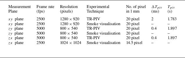
The experimental images are recorded at different image resolutions and frame rates in different measurement planes depending on the TR-PIV and flow visualisation requirements and constraints. The image recording details for each measurement plane and measurement technique are mentioned in table 1. The post-processing of TR-PIV images was carried out using VidPIV, a commercial software from Oxford Lasers. A cross-correlation scheme is applied on an interrogation window size of
 $64\times 64$
pixel
 $^{2}$
with
 $50\,\%$
overlap. The cross-correlated data are corrected twice using the local velocity filter and outlier interpolation. The interrogation widow is then reduced to a size of
 $32\times 32$
pixel
 $^{2}$
and an adaptive cross-correlation scheme is applied on the reduced size window with 50 % overlap. The outliers are interpolated after the local velocity filtering and the process is repeated a few times. A velocity smoothing operation is carried out at the final step to generate the final vector map. The PIV image processing tree remains the same for all test cases and all the measurement planes.
Details of image recording parameters. Here, fps stands for frames per second,
 $ \Delta T_{piv}$
is the time interval between two consecutive PIV image pairs and
 $ T_{piv}$
is the total recording time for TR-PIV measurement.

2.3. Phase-averaging and test conditions
The flow field generated by the DBD-PA can be divided into three regimes: (i) starting flow; (ii) transitional flow; and (iii) periodic flow (Mishra & Panigrahi Reference Mishra and Panigrahi2024). The periodic flow characteristics are discussed using instantaneous smoke visualisation images and phase-averaged PIV results. The phase-averaging is carried out by extracting the same phase data from the sequentially recorded data. The periodic flow is attained after a few hundred milliseconds have elapsed. Therefore, the periodic flow data remain available for at least approximately one second (see table 1 for total recording time) for phase averaging. In the periodic flow regime, the flow field generated by the DBD-PA is locked in with the burst frequency. The repeatability of the flow field in each burst cycle has been verified by carefully examining the instantaneous flow field over several burst cycles for each test condition in each measurement plane. The instantaneous flow field repetition is confirmed by matching the vortex core locations, velocity magnitude at the exact location and total flow field distribution. The phase-averaged data were compared with the instantaneous data in several cycles. A negligible difference is observed between the phase-averaged and instantaneous data for all the measurement planes.
Since the total recording time is fixed, the total number of vector fields available for the phase averaging at a given phase varies with
 $ f_{b}$
. Another constraint is imposed by the time interval between two consecutive PIV image pairs
 $ \Delta T_{piv}$
and
 $ t_{b}$
. The division of
 $ t_{b}$
by
 $ \Delta T_{piv}$
should be an integer for averaging. For example, the value of
 $ t_{b}/ \Delta T_{piv}$
with
 $ t_{b} = 25$
ms (case 4) and
 $ \Delta T_{piv} =2$
ms is non-integer. In such cases, the next cycles are skipped until an integer value is obtained and the number of vector fields available for the phase-averaging at a given phase decreases. The starting flow phenomenon in this paper is discussed using instantaneous data. This is because obtaining the same quiescent condition is inconvenient and difficult. However, in such situations, the accuracy and repeatability of the flow field phenomenon can be confirmed by repeating the measurements. We have ensured it by repeating the visualisation multiple times and acquiring the PIV data twice for all the burst mode test conditions.
As mentioned in § 2.1, the actuator is operated in continuous and burst modes. The AC input signal amplitude,
 $\phi _{pp}=14$
kV, and frequency,
 $f_{ac}=2$
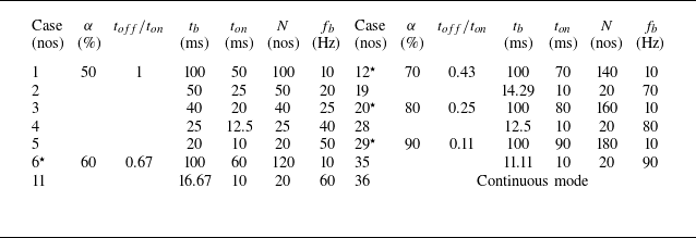
kHz, are kept constant. The generation of periodic vortex is controlled by controlling burst signal parameters. Table 2 provides detailed information on the experimental test conditions. The highest
 $ f_{b}$
is fixed at 90 Hz as at higher burst frequency,
 $ f_{b}\gt 100$
Hz, the DBD-PA induced flow approaches that of the continuous mode (Santhanakrishnan & Jacob Reference Santhanakrishnan and Jacob2007; Santhanakrishnan et al. Reference Santhanakrishnan, Reasor and LeBeau2009; Emori et al. Reference Emori, Kaneko and Nishida2022; Mishra et al. Reference Mishra, Gupta and Panigrahi2022). The lower limit of the duty cycle is fixed at 50 % because the duty cycle of
 $ \leqslant 50\,\%$
will lead to idle time greater than the ON time and there will be negligible vortex interaction. The test conditions for the spanwise measurements (listed in table 2) were finalised based on the insight gained from several longitudinal plane measurements by operating the actuator in burst mode for
 $50\,\% \leqslant \alpha \leqslant 90\,\%$
and 10 Hz
 $\leqslant f_{b} \leqslant 90$
Hz detailed by Mishra & Panigrahi (Reference Mishra and Panigrahi2024).
Details of experimental test conditions for measurements. The actuation voltage amplitude,
 $\phi _{pp}=14$
kV, and frequency,
 $f_{ac}=2$
kHz, are kept constant. The superscript star (
 $ ^{\star }$
) indicates that measurements are taken only for the longitudinal plane. Here,
 $ N$
is the number of AC cycles in one burst cycle and the other signal parameters are defined in figure 1(b).

2.4. Error and uncertainty
The spatial resolution of PIV images is equal to 0.05 mm. Due to windowing, the actual spatial resolution of PIV data is reduced to 0.8 mm after PIV image processing. The uncertainty in velocity measurements obtained from PIV measurements can be estimated as
 $ u_{e} = \sqrt {({d_{e}^{2}}/{t_{p}^{2}}) + (-({d}/{t_{p}^{2}} )^{2}t_{e}^{2})}$
(Dong, Choi & Wang Reference Dong, Choi and Wang2022), assuming that its primary sources of error are the seeding particle shift distance,
 $ d$
, and the laser pulse separation time,
 $ t_{p}$
. Here,
 $ d_{e}$
is the uncertainty associated with
 $ d$
, which is typically 0.2 pixel (Westerweel Reference Westerweel2000). The uncertainty in laser pulse separation time
 $ t_{e}$
remains of the order of a few nanoseconds or even less and can be neglected in low-speed flow. For the longitudinal plane, it gives the uncertainty in velocity,
 $ u_{e} = 0.025$
ms−1, which is less than 5 % of 0.52 ms−1, which is the lowest global maximum velocity observed in the mean flow for Case 1. The uncertainty in the velocity measurements of spanwise planes is twice that of the longitudinal plane, i.e.
 $ u_{e} = 0.05$
ms−1. This is because the spatial resolution for TR-PIV is the same and the laser pulse separation frequency (equal to the frame rate of image recording) for spanwise planes is twice that of the longitudinal plane. Although the absolute value of uncertainty is greater in the spanwise measurement planes, the percentage of error with respect to the maximum velocity remains lower because the magnitude of maximum velocity in the spanwise measurement plane is higher. All the experiments were carried out in an air-conditioned room with a room temperature maintained at approximately 20 °C for constant ambient conditions.
3. Results and discussion
The results from the present study are discussed in the following three parts: (a) flow visualisation; (b) vortex dynamics; and (c) instability mechanism.
3.1. Flow visualisation
Instantaneous smoke visualisation images of the periodic vortex in the longitudinal
 $ (xy)$
plane (at the same phase): (a) 20 ms after the start of burst cycle as a function of
 $ f_{b}$
at
 $ \alpha = 50\,\%$
and (b) 40 ms after the start of burst cycle, as a function of
 $ \alpha$
at
 $ f_{b} = 10$
Hz. It may be noted that the axis limits are different in panels (a) and (b).

The planar flow visualisation images can provide details of the geometrical features of the vortices during evolution and transport. The phase-referenced flow visualisation images of the periodic vortex for different longitudinal, transverse and horizontal planes are presented in this section. The flow structures are shown using the instantaneous visualisation images. The repeatability of the flow structures in these visualisation images have been confirmed from repeated measurements at different time instants with the same actuator and different actuator. More details on the dynamics of the vortex evolution can be obtained from the movies in the supplementary material available at https://doi.org/10.1017/jfm.2025.198.
3.1.1. Longitudinal plane visualisation
Figure 3 shows the instantaneous smoke visualisation images of the periodic vortex as a function of
 $ f_{b}$
and
 $ \alpha$
in the longitudinal plane (
 $xy$
). Figure 3(a) demonstrates the effect of
 $ f_{b}$
at a constant duty cycle of 50 %. The periodic vortex structure is shown for five different values of
 $ f_{b}$
ranging from 10 Hz to 50 Hz at the same phase, i.e. 20 ms after the start of the burst cycle. The vortex originates at the exposed electrode (see annotated visualisation at 10 Hz in figure 3
a) and convects along the wall at some angle
 $ \theta$
measured with respect to the wall surface. The vortex core location is marked with a white dot and denoted as
 $ x_{c}$
and
 $ y_{c}$
for horizontal and vertical coordinates, respectively. A clear difference in the periodic vortex behaviour can be observed at higher values of
 $ f_{b}$
. The periodic vortex structure is similar for lower and moderate values of burst frequency, i.e. for
 $ f_{b}=10$
Hz, 20 Hz and 25 Hz. However, the vortex topology changes at greater values of
 $ f_{b}=40$
Hz and 50 Hz. The downstream part of the periodic vortex rolls up in a clockwise direction, forming a dipole-like structure. The dipole formation takes place due to the boundary layer roll-up. The periodic vortex size is gradually reduced with increasing burst frequency. The vortex core is also located farther downstream for higher values of
 $ f_{b}$
. It indicates that the core velocity is a function of
 $ f_{b}$
. The upstream shear layer roll-up (spiral) behaviour is the same at all the values of
 $ f_{b}$
. The vortex topology is modified in the near-wall downstream region due to the interaction of the periodic vortex with the preceding vortex. These observations suggest that the burst frequency can control the periodic vortex size, speed, core trajectory and morphology.
Figure 3(b) demonstrates the effect of
 $\alpha$
at a constant burst frequency of 10 Hz. The periodic vortex is shown at the same phase, i.e. after 40 ms from the start of the burst cycle, for five different values of
 $ \alpha$
ranging from 50 % to 90 %. It may be noted that the axis limits are not the same in figures 3(a) and 3(b). Figure 3(b) indicates that the duty cycle does not influence the overall structure of the periodic vortex. The vortex size grows with an increase in
 $ \alpha$
in contrast to an increase of
 $ f_{b}$
. This can be verified by comparing the vortex sizes at
 $ \alpha =50\,\%$
and 90 %. The vortex core is located farther downstream and closer to the wall at higher duty cycle (see
 $ \alpha =80\,\%$
and 90 %). This means the vortex core travels at a small angle
 $ \theta$
relative to the wall for large duty cycles. It also indicates that the vortex core velocity and trajectory are both influenced by the duty cycle. The fluid present downstream of the periodic vortex is due to the remnant vortex. More remnant fluid is present at the higher duty cycle. This is because a higher duty cycle corresponds to a shorter idle time. A similar effect can be observed for higher values of
 $ f_{b} =$
40 Hz and 50 Hz (see figure 3
a) where the absolute value of idle time is small because
 $ t_{b}$
is small. An identical observation was made in the previous work from the Schlieren measurements (Mishra & Panigrahi Reference Mishra and Panigrahi2017a
). Similar results confirm the accuracy of both measurement techniques and justify the negligible influence of seeding on the induced flow under the action of the electric field. Figure 3 confirms that the nature of periodic vortex structures is a strong function of
 $ f_{b}$
. Therefore, the role of
 $ f_{b}$
is investigated using the spanwise measurements in transverse and horizontal planes (see table 2), which have been presented in the following sections.
Instantaneous smoke visualisation images of the periodic flow in transverse
 $ (zy)$
plane fixed at a distance of
 $x=10$
mm as a function of
 $ f_{b}$
, with
 $ \alpha =50\,\%$
. The results are shown at two different time instants,
 $t=$
 $t_{0}-\Delta t$
and
 $t_{0}$
, where
 $t_{0}$
is the time instant at which the measurement plane intersects the vortex core centre and
 $\Delta t$
is equal to 3.2 ms.

Instantaneous smoke visualisation images of the periodic flow in the
 $zy$
plane at a distance of
 $x=20$
mm as a function of
 $ f_{b}$
, with
 $ \alpha =50\,\%$
. The results are shown for two different time instants,
 $t=$
 $t_{0}-\Delta t$
and
 $t_{0}$
, where
 $t_{0}$
is the time instant at which the vortex core intersects the selected measurement plane and
 $\Delta t$
is equal to 6.2 ms.

3.1.2. Transverse plane visualisation
Figures 4 and 5 show the instantaneous smoke visualisation images as a function of
 $ f_{b}$
in the transverse plane (
 $zy$
) fixed at
 $ x=10$
mm and
 $ x=20$
mm, respectively. The visualisation images of the moving vortex at two different instants,
 $ t=t_{0}-\Delta t$
and
 $ t=t_{0}$
, are shown, where
 $ t_{0}$
refers to the time instant when the vortex core intersects the selected measurement plane. At
 $ t=t_{0}-\Delta t$
, the vortex enters the measurement plane, where
 $ \Delta t$
is equal to 3.2 ms. Cell structures are formed due to spanwise instability present in the form of waves on the vortex periphery. The wave-like cell structures are initiated at
 $ f_{b} = 10$
Hz. At the moderate range, 10 Hz
 $\lt f_{b}\lt$
40 Hz, the structures start separating from each other. This may be attributed to the increase in wave amplitude with the increase in burst frequency. The series of cell structures remain well organised over the entire span. The cell structures are separated at similar distances over the span (see the annotation in the visualisation images shown for 25 Hz at
 $ t=t_{0}-\Delta t$
). A typical distance of 5 mm is observed containing one pair of cell-like structures for 10 Hz
 $\lt f_{b}\lt$
40 Hz. It indicates that the spanwise wavelength is almost independent of
 $ f_{b}$
. At
 $ t=t_{0}$
, the formation of small streamwise vortices is observed at the top edge of the cell-like structures. The middle region (marked with a dotted line) corresponds to the vortex core, which remains nearly straight for
 $ f_{b}\lt 25$
Hz. At
 $ f_{b} =$
40 Hz and 50 Hz, an instability wave appears in the vortex core region.
Figure 5 shows the spanwise structure of the periodic vortex in the downstream region i.e. transverse plane at
 $ x=20$
mm. At
 $ t=t_{0}-\Delta t$
, the cell structures observed at
 $ x=10$
mm are no longer present. However, several streamwise vortices are present which were in the nascent stage at
 $ x=10$
mm (see figure 4). They grow downstream and appear in pairs of counter-rotating vortices (vortex dipole) akin to mushroom-like structures. The streamwise vortex pairs are connected to each other like a string. The spanwise structure of a larger periodic vortex (corresponding to low
 $ f_{b}\lt 25$
Hz) is observed to be similar to the spanwise structure of the junction vortex reported by Allen & Naitoh (Reference Allen and Naitoh2007). The vortex core becomes irregular in comparison to the vortex core observed at
 $ x=10$
mm because of the instability growth. At
 $ f_{b} =40$
Hz, the vortex core is nearly diffused. The extent of vortex cross-section and spanwise structure in the wall-normal distance indicates the periodic vortex size reduces with an increase in burst frequency similar to the observation in the longitudinal plane (see figure 3).
3.1.3. Horizontal plane visualisation
Figures 6 and 7 show the instantaneous spanwise structure of the periodic vortex in the horizontal plane
 $(zx)$
fixed at
 $ y=3$
mm and 6 mm, respectively. Three different time instants are selected to demonstrate the instability development i.e.
 $ t/t_{v} =0.25, 0.5$
and 0.75, where
 $ t_{v}$
is the vortex residence time in the respective plane. The vortex residence time
 $ t_{v}$
is calculated by observing the sequential flow visualisation images. The time
 $ t/t_{v}=0$
is the time when the smoke sheet corresponding to the front edge of the vortex approaches the measurement plane and
 $ t/t_{v}=1$
is the time when the smoke trace corresponding to the rear edge of the vortex leaves the respective measurement plane. Figure 6 demonstrates a wavy pattern in the downstream edge with mushroom-shaped vortices. The waviness corresponds to the outer turn of the periodic vortex and may be related to the instability wave development due to which the mushroom vortices are generated. The wider and nearly straight strip of finite width corresponds to the vortex core region. The visualisation images reveal that the vortex core remains nearly straight in the spanwise direction at all burst frequencies, except for
 $ f_{b} =50$
Hz, where minor oscillation can be observed in the core region. The vortex core resides in the plane for a shorter time interval at lower burst frequency values than the higher burst frequency. This is because of the difference in vortex size and the core travelling angle,
 $ \theta$
, which is higher for lower values of
 $ f_{b}$
. The downstream wavy structures start decaying at a lower burst frequency and diffuse for
 $ f_{b} =40$
Hz and 50 Hz. This may be attributed to the roll-up of the boundary layer, resulting in the formation of dipoles. The vortex core also resides in the plane for a longer time for
 $ f_{b} =40$
Hz and 50 Hz due to the smaller core travelling angle. Figure 7 shows the instantaneous visualisation images in the horizontal (
 $ xz$
) plane at
 $y=6$
mm. The vortex core width is greater at
 $y=6$
mm compared with that at
 $y=3$
mm. This is due to the spatial growth of the vortices away from the wall. The oscillation present in the vortex core for
 $ f_{b} =50$
Hz at
 $ t/t_{v}=0.25$
is temporally damped at
 $ t/t_{v}=0.5$
and 0.75 indicating that the vortex tends to stabilise with time. However, some minor fluctuations can still be observed in the vortex for
 $ f_{b} \geqslant 20$
Hz. A comparison of figure 7 with figure 6 reveals that waves appear on the travelling vortices both in front and back regions during their development in space and time. The waves in the front part of the vortex demonstrate greater growth in the wall-normal direction compared with that of the vortex in the rear part. The comparison of figures 4 and 5 with figures 6 and 7 indicates that the mushroom-like vortex structures seen in the outer regime of the developing vortex in the
 $ zy$
and
 $ zx$
planes are correlated with each other.
Instantaneous smoke visualisation images of the periodic vortex in the horizontal
 $ (zx)$
plane fixed at
 $y=3$
mm as a function of
 $ f_{b}$
at
 $ \alpha =50\,\%$
. The values of residence time,
 $t_{v}$
(ms), are 12, 12, 10, 8 and 16 for an
 $ f_{b}$
(Hz) of 10, 20, 25, 40 and 50, respectively. The residence time
 $t_{v}$
is the duration of the flow structure in the respective plane. The time
 $t=0$
is set at the instant when the vortex approaches the selected plane.

3.2. Vortex dynamics
In this section,
 $ xy$
plane measurements are used to demonstrate the periodic vortex formation and evolution. The development of the starting vortical structure, merging of the first vortex with the second vortex and formation of the periodic vortices are presented. The effect of burst frequency on periodic vortex characteristics is highlighted and comments on self-similarity are made. The vorticity distribution of the periodic vortex is also analysed and compared with the theoretical prediction.
Instantaneous smoke visualisation images of the periodic vortex in the horizontal
 $ (zx)$
plane fixed at
 $y=6$
mm as a function of
 $ f_{b}$
at
 $ \alpha =50\,\%$
. The values of residence time,
 $t_{v}$
(ms), are 43.2, 30.8, 30.4, 24, and 20.8 for an
 $ f_{b}$
(Hz) of 10, 20, 25, 40 and 50, respectively. The residence time
 $t_{v}$
is the duration of the flow structure in the respective plane. The time
 $t=0$
is set at the instant when the vortex approaches the selected plane.

3.2.1. Starting flow and vortex merging
Development of the starting flow in burst mode for
 $ f_{b}=50$
Hz and
 $ \alpha =50\,\%$
. Instantaneous velocity vectors are superimposed on vorticity,
 $ \Omega _{z}$
(s−1), with a common contour scale at all the time instants. The actuation signal is shown at the top of the contour plot for reference and the end of each burst cycle is marked with a filled circle (red in colour) where
 $ t_{b}$
is the burst cycle period.

The starting flow induced by a burst-modulated DBD-PA at higher burst frequencies is composed of several vortices. The vortices merge with each other and the total number of vortices involved in the merging process is a function of the burst cycle parameters. Figure 8 shows the development of starting flow at the end of each burst cycle for a burst modulated DBD-PA operating at
 $ f_{b}=50$
Hz and
 $ \alpha =50\,\%$
with the help of velocity vectors superimposed on isocontours of axial vorticity,
 $ \Omega _{z}$
(s−1). The flow field results are presented for nine subsequent burst cycles from
 $ t/t_{b}=1$
to 9, where
 $ t/t_{b}=0$
corresponds to the start of actuation. At
 $ t/t_{b}=1$
, we can observe the presence of a single vortex generated during the first burst cycle which is known as the starting vortex. A vortex of greater size and higher strength is observed at
 $ t/t_{b}=2$
. This is due to the starting vortex merging with the second vortex generated during the second burst cycle. This happens quickly as the second vortex travels faster than the first vortex (Mishra & Panigrahi Reference Mishra and Panigrahi2017a
). Similarly, the third vortex is also merged at the end of the third burst cycle. Consequently, the vorticity magnitude and size of the resulting vortex are further increased. The vorticity distribution inside the vortex keeps changing because of the vortex merging. It may also be observed that the orientation of the velocity vectors at
 $ t/t_{b}=2$
and 3 is not the same as that at
 $ t/t_{b}=1$
.
As time progresses, the vortex moves downstream, and the distance between the remnant vortex and the exposed electrode increases. The remnant vortex keeps moving due to self-induced velocity even when no plasma actuation exists. Consequently, the subsequently generated vortices could not complete the merging process because they must travel more to reach the remnant vortex core. For example, at
 $ t/t_{b}=4-6$
, one can observe two patches of peak vorticity. At later times (
 $ t/t_{b}=7-9$
), the resultant vortical structure ingests the incipient vortices. Overall, figure 8 demonstrates that the vortices generated by the actuator in each burst cycle during the initial period merge at the end of the burst cycle. Finally, a large vortical structure is developed, leading to the quasi-periodic flow.
Merging process of the second vortex with the starting vortex. The instantaneous flow field is shown using the velocity vectors superimposed on isocontours of negative values of
 $\lambda _{2}$
(s
 $ ^{-2}$
). The burst mode operating parameters are
 $ f_{b} =25$
Hz and
 $ \alpha =50\,\%$
. The
 $\lambda _{2}$
contours labelled as 1 and 2 indicate vortex 1 (starting vortex) and vortex 2 (second vortex), respectively.

We now select the first two consecutive burst cycles
 $ (t/t_{b} \leqslant 2.05)$
to describe the vortex merging phenomenon. Figure 9 demonstrates the vortex merging process of the starting vortex and the second vortex when the actuator is working at
 $f_{b}=25$
Hz with a duty cycle of 50 %. The core of the vortex or coherent structure can be identified using the properties of the velocity gradient tensor. The
 $ Q$
-criterion (Hunt et al. Reference Hunt, Wray and Moin1988) and
 $ \lambda _{2}$
-criterion (Jeong & Hussain Reference Jeong and Hussain1995) are widely used techniques for identifying the vortical structures. Jeong & Hussain (Reference Jeong and Hussain1995) demonstrated that the
 $\lambda _{2}$
-criterion outperforms the other vortex identification technique. In the planar flows, the regions defined by
 $ -\lambda _{2}$
and
 $ +Q$
are equivalent (Jeong & Hussain Reference Jeong and Hussain1995). The vortex merging process is described using the
 $ \lambda _{2}$
-criterion evolution. Figure 9 shows the instantaneous flow field using the velocity vectors superimposed on isocontours of
 $\lambda _{2}$
-criterion for six sequential time instants
 $ t/t_{b}=1.4-2.05$
. At
 $ t/t_{b} =1.4$
, the contours of
 $ \lambda _{2}$
explicitly present two co-rotating (same sign of vorticity) vortices. The starting vortex is labelled as ‘1’, and the second vortex is marked as ‘2’. As the second vortex convects downstream, the distance between vortex 1 and vortex 2 decreases. At
 $ t/t_{b} =1.65$
, vortex 2 comes closer to vortex 1. Vortex 1 and vortex 2 co-rotate at
 $ t/t_{b} =1.75$
and mutual interaction occurs between the two vortices. While co-rotating, vortex 2 becomes stronger and vortex 1 becomes weaker, as apparent from the magnitude of
 $ \lambda _{2}$
at
 $ t/t_{b} =1.75$
and 1.85. It may be noted that plasma forcing is stopped at
 $ t/t_{b} =1.5$
. Finally, vortex 1 and vortex 2 completely merge at
 $ t/t_{b} =2.05$
.
It is well known that the co-rotating vortices eventually merge to form a single vortex. Cerretelli & Williamson (Reference Cerretelli and Williamson2003) explained the physical mechanism behind the vortex merging using the vorticity field decomposition (described later in § 3.3.2) into symmetric and anti-symmetric components. The anti-symmetric vorticity field causes the co-rotating vortices to be pushed towards each other during the merging process. The anti-symmetric vorticity comprises two counter-rotating vortex pairs and their induced velocity readily pushes the two vortex centres to bring them together, leading to vortex merging. The critical ratio of core size,
 $ a_{c}$
, and separation distance,
 $ l_{c}$
, at which merging starts, is experimentally observed as
 $ a_{c}/l_{c} = 0.29\pm 0.01$
(Meunier & Leweke Reference Meunier and Leweke2001) and
 $ a_{c}/l_{c} = 0.24\pm 0.01$
(Meunier et al. Reference Meunier, Ehrenstein, Leweke and Rossi2002) for the merging of a pair of equal two-dimensional co-rotating vortices generated by impulsively rotated flat plates. We calculated the critical ratio at
 $ t/t_{b} = 1.4$
, 1.5 and 1.65, which gives
 $ a_{c}/l_{c} = 0.22\pm 0.01$
. A similar critical ratio of vortex core size and separation distance confirms the similarity of the vortex merging process in the DBD-PA to that of impulsively rotating flat plates. The minor difference in the value of the critical ratio may be attributed to the unequal strength of the vortex 1 and vortex 2 because they are generated at different instants.
Formation of the periodic vortex from starting vortex for two different values of
 $ \alpha =50\,\%$
and 80 % at
 $ f_{b}=10$
Hz. The instantaneous isocontours of
 $ \Omega _{z}$
are shown for the first four consecutive burst cycles at the same phase,
 $ t/t_{b}=0.4$
. The contour levels are the same for each plot. The vortex core location is marked using a plus sign and mentioned inside the respective plot.

3.2.2. Formation of periodic vortices
The starting vortex is generated in a quiescent environment and the subsequent vortices generated during the burst cycle are exposed to the remnant flow from previous cycles. Figure 10 shows the comparison of vortices generated during four consecutive burst cycles from the start of the actuator for two different values of
 $ \alpha =50\,\%$
and 80 %, at a constant value of
 $ f_{b} =10$
Hz. The results are shown using the instantaneous flow field at the same phase, i.e.
 $ t/t_{b}=0.4$
, with the help of isocontours of vorticity,
 $ \Omega _{z}$
. For both values of
 $ \alpha$
, the starting vortex core is located nearly at the same location. The near-wall negative vorticity wraps the outer part of vortices in the upstream region, and the highest shear occurs at the interface of positive and negative vorticity. The vortices generated after the starting vortex are located farther downstream with respect to the starting vortex core location. There are minor differences between the structure and core location of the third vortex and fourth vortex for both duty cycles. The second vortex core is located farther downstream than the rest of the vortices. This is due to the mutual interaction between the starting vortex and the second vortex, which is similar to the leapfrogging of vortex rings. The leapfrogging phenomenon occurs when two identical coaxial vortex rings move along a common axis. Due to their mutual interaction, the leading vortex ring causes the rearward ring to shrink and accelerate. Consequently, the rearward ring moves faster. Concurrently, the induced velocity of the rearward ring causes the leading ring to grow and decelerate (Yamada & Matsui Reference Yamada and Matsui1978; Cheng et al. Reference Cheng, Lou and Lim2015) .
The second vortex travels farther downstream for
 $\alpha =80\,\%$
compared with that for
 $\alpha =50\,\%$
. The core of the third and fourth vortex is also located farther downstream for
 $\alpha =80\,\%$
than that for
 $\alpha =50\,\%$
. It indicates that a higher duty cycle increases the vortex core velocity. The geometric shape of the periodic vortex for
 $\alpha =80\,\%$
is also different. The vorticity distribution shows a circular pattern for the periodic vortex generated at
 $ \alpha =50\,\%$
and elliptic for
 $ \alpha =80\,\%$
(see the black dashed closed curve of the fourth vortex in figure 10). For a given
 $ f_{b}$
, the value of
 $\alpha$
determines the net energy addition per burst cycle and the time delay between the generation of the two consecutive vortices. A greater
 $ \alpha$
for a given
 $ f_{b}$
allows more time for the actuator to remain ON and a short idle time, increasing the net momentum exchange with the ambient fluid. This results in an increased convection speed of the vortex and greater vortex interaction (Mishra & Panigrahi Reference Mishra and Panigrahi2018).
The
 $ u$
-velocity profile along (a) the streamwise
 $x$
-direction at
 $ y=5.2$
mm and (b) wall-normal
 $y$
-direction at
 $ x=6.2$
mm showing the differences in remnant flow from the start of the second vortex onward till the eighth vortex for
 $ \alpha =50\,\%$
and
 $ f_{b} =10$
Hz.

The differences between subsequent vortex structures are attributed to the initial conditions at the generation of the subsequent vortices. The differences in initial flow conditions at the start of each burst cycle can be better understood with the help of the velocity profiles extracted near the exposed electrode. Figure 11 shows the
 $ u$
-velocity profile at seven subsequent time instants just before the start of actuation in each burst cycle for
 $ \alpha =50\,\%$
and
 $ f_{b} =10$
Hz. The initial conditions are shown for the second burst to the eighth burst, i.e. at
 $ t_{0}+t_{b}-\Delta t$
to
 $ t_{0}+7t_{b}-\Delta t$
, where
 $ t_{0}$
refers to the start of the actuator and
 $ \Delta t=2$
ms is a constant. The profile is extracted along the streamwise distance at a fixed wall-normal distance of
 $ y=5.2$
mm and at a fixed streamwise distance of
 $ x=6.2$
mm.
It can be noticed that the velocity profiles during
 $5^{th}$
to
 $8^{th}$
vortex cycle overlap with each other in both streamwise and wall-normal directions. This data collapse indicates no change in initial remnant flow conditions for these burst cycles. The differences occur between
 $2^{nd}$
to
 $5^{th}$
vortex profile. A large deviation in velocity is observed in the downstream region and away from the wall. The velocity profile in the streamwise direction indicates that the second vortex velocity is higher in the region of
 $ 14\lt x\lt 24$
mm. The velocity profile in the wall-normal distance also indicates that the second vortex velocity has the greatest magnitude near the wall. This higher magnitude of velocity gradually reduces until the fifth profile. For the fifth to eighth vortex profile, there is a negligible difference in the near-wall region (up to
 $ y=12$
mm). Further away from the wall,
 $ 12\lt y\lt 25$
mm, the differences are still more significant in the case of the second vortex profile. This difference indicates that flow conditions are quite different near the exposed electrode before the start of the second burst cycle. This means that the second vortex is created in the fastest-moving remnant flow, which travels faster than the rest of the subsequent vortices. The small difference at later time instants suggests that vortices generated after the third vortex can be treated as repeating or periodic (or quasi-periodic) vortices at low and moderate burst frequencies.
Periodic flow vortex core trajectory
 $ (x_{c},y_{c})$
over six consecutive burst cycles in the
 $xy$
plane, for (a)
 $ f_{b} =10$
Hz and (b) 20 Hz at a constant value of
 $ \alpha =50\,\%$
. The average value of the vortex core travelling angle
 $ \theta$
is mentioned inside the respective plot at the top left corner.

3.2.3. Core trajectory of periodic vortices
Figure 12 shows the trajectory of the periodic vortex core in the
 $ xy$
plane over six consecutive burst cycles, for
 $ f_{b} =10$
Hz and 20 Hz at a constant value of
 $ \alpha =50\,\%$
. The centre of the peak vorticity region is considered as the location of the vortex core. The core travelling angle,
 $ \theta$
(also refer to figure 3) is calculated as
 $ \theta =\tan ^{-1}(y_{c}/x_{c})$
. The vortex core travels at a smaller angle for the higher value of
 $ f_{b}$
. The periodic vortex for
 $ f_{b} =10$
Hz travels at an angle,
 $ \theta$
, of 29.8°. However, it travels at an angle of 22.7° for
 $ f_{b} =20$
Hz. For a greater value of burst frequency,
 $ \theta$
is reduced further to a lower value. The decrease in values of
 $ \theta$
is due to faster movement of the vortex in the streamwise direction and slower movement in the vertical direction for greater values of
 $ f_{b}$
. The starting vortex in the continuous mode travels at an angle of 31° (Whalley & Choi Reference Whalley and Choi2012). The periodic vortex travels at an angle smaller than that of the starting vortex (Mishra & Panigrahi Reference Mishra and Panigrahi2017a
). Xue et al. (Reference Xue, Gao, Xi and Liu2020) reported that vortex core travelling angle decreases from 23° to 17° as
 $ f_{b}$
increases from 5 to 50 Hz. In the present study, we also observe a similar behaviour and nearly the same value of
 $ \theta = 17$
° at
 $ f_{b}=50$
Hz and
 $ \alpha =50\,\%$
.
At higher values of
 $ f_{b}$
, the vortex size is small and these small vortices march parallel to the wall due to less momentum transfer because of the shorter duration of plasma-generated forcing. This is the reason behind a long residence time of the spanwise core structure at higher values of
 $ f_{b}$
, as observed in figures 6 and 7. The scatter in the core trajectory is attributed to the nature of the periodic vortex, which is different in each burst cycle due to the nonlinear interaction of the periodic vortex with the remnant flow. The core location is more scattered in the downstream region due to greater unsteadiness attributed to the diffusion of the periodic vortex with the remnant flow.
3.2.4. Self-similarity of periodic vortices
The characteristics of the vortex generated due to impulsive action are self-similar over a time interval if scaled by proper scaling parameters. Cantwell (Reference Cantwell1986) reported a detailed mathematical treatment of the transient motion when a viscous incompressible fluid is forced from an initial state of rest. The self-similarity parameters derived by Cantwell (Reference Cantwell1986) have been used to test the self-similar behaviour of impulsively generated vortices such as junction vortex (Allen & Lopez Reference Allen and Lopez2007; Allen & Naitoh Reference Allen and Naitoh2007), starting vortex (Whalley & Choi Reference Whalley and Choi2012; Mishra & Panigrahi Reference Mishra and Panigrahi2017a ) and periodic vortices (Mishra & Panigrahi Reference Mishra and Panigrahi2017a ). The self-similarity parameters for space and velocity are given as follows:
 \begin{equation} \xi = \frac {x}{M^{1/3}t^{q/3}}\,, \quad \eta = \frac {y}{M^{1/3}t^{q/3}}\,, \quad \zeta = \frac {u}{M^{1/3}t^{(q/3)-1}}, \end{equation}
where
 $ M$
is the amplitude parameter for the force acting on the fluid,
 $ q$
is the forcing parameter, and
 $ q = 1,2$
and 3 for impulse, constant (step) and ramp forcing (Cantwell Reference Cantwell1986). We assume
 $M\sim \nu U_{a}$
and
 $q=2$
for (3.1), where
 $ U_{a}$
is the average velocity of the time-averaged mean flow field. The average velocity is calculated as
 $ U_{a} = U_{max}/2$
, where
 $ U_{max}$
is the absolute maximum of
 $ u$
-velocity in the time-averaged mean flow field. It may be noted that instead of
 $ U_{a}$
, vortex core velocity
 $ u_{c}$
was used in our earlier investigation (Mishra & Panigrahi Reference Mishra and Panigrahi2017a
). However, it is observed that
 $ U_{a}$
is nearly the same as that of
 $ u_{c}$
. The time can be made non-dimensional using the definition,
 $ t^{*} = tU_{a}^{2}/\nu$
, where
 $ \nu$
is the kinematic viscosity of the fluid. The non-dimensional time is an equivalent of Reynolds number (Allen & Naitoh Reference Allen and Naitoh2007).
Phase-averaged flow field in similarity coordinates
 $ (\xi ,\eta )$
with self-similar velocity parameter
 $ (\zeta )$
at some selected non-dimensional time interval,
 $ t^{*}$
, for different values of burst frequency: (a) 10 Hz; (b) 25 Hz; and (c) 40 Hz. The duty cycle
 $ \alpha =50\,\%$
is constant. The periodic vortex core location,
 $ (\xi _{c},\eta _{c})$
, is marked using a black dot with the respective value mentioned inside the brackets.

Figure 13 shows the periodic vortex evolution in similarity coordinates
 $ (\xi ,\eta )$
for three different values of
 $ f_{b}=10$
Hz, 25 Hz and 40 Hz using the phase-averaged data. The velocity vectors are superimposed on the isocontours of
 $ \zeta$
and the results are presented for nearly the same values of
 $ t^{*}$
. The vortex core location in the similarity coordinates (
 $ \xi _{c},\eta _{c}$
) corresponding to (
 $x_{c},y_{c}$
) in the absolute coordinates is identified by the visual inspection of velocity vectors on similarity coordinates and marked with a black dot. The respective coordinate values are also mentioned inside the plots. It should be noted that the flow field presented in figure 13 for the vortex characterisation contains more than one vortex. However, the self-similar parameters are valid for the incipient vortex present in the upstream region. For
 $ f_{b}=10$
Hz, the core location occurs at
 $ (0.89,0.51)$
for
 $ t^{*} = 208$
and at
 $ (0.89,0.47)$
for
 $ t^{*} = 286$
. It can be noticed from the vortex core trajectory presented in figure 12 that the core location in the
 $ y$
-direction is undulating in nature. The lower value of
 $ \eta _{c} = 0.47$
at the later time can be due to these undulations. The undulations in the core trajectory are possible if the vortex core oscillates along its rotation axis. The starting vortex core location remains constant at
 $ (0.7,0.52)$
(Whalley & Choi Reference Whalley and Choi2012). For
 $ f_{b}=25$
Hz, the value of
 $ (\xi _{c},\eta _{c})$
is
 $ (1.1,0.45)$
at
 $ t^{*} = 209$
. For
 $ f_{b}=40$
Hz, we have marked two core locations
 $ (0.72,0.3)$
at
 $ t^{*} = 52$
and
 $ (1.3,0.48)$
at
 $ t^{*} = 210$
corresponding to incipient vortex and remnant vortex, respectively. It can be noticed that the core location of vortex for
 $ f_{b}=40$
Hz at
 $ t^{*} = 210$
is obscure. It may be noted that the values of
 $ \xi _{c}$
and
 $\eta _{c}$
from the phase-averaged data match well with those from the instantaneous data.
The differences between the core locations for nearly the same
 $ t^{*}$
at different burst frequencies can be attributed to the change in their velocity magnitude. This is also evident from the reduction in peak values of
 $ \zeta$
for 25 Hz and 40 Hz burst frequency. For
 $ f_{b}=10$
Hz, the value of
 $ t$
is large and convection velocity,
 $ U_{a}$
, is small, and for a greater value,
 $ f_{b}=25$
Hz and 40 Hz, the value of
 $ t$
is small and
 $ U_{a}$
is greater in magnitude. The vortex core location in the streamwise direction,
 $ \xi _{c}$
, shifts to the higher side for a greater vortex convection velocity. Thus, it indicates that the core location of the impulsively created periodic vortex on the similarity coordinates changes with the operating conditions. For a given duty cycle,
 $ \xi _{c}$
increases and
 $ \eta _{c}$
decreases with increasing burst frequency. A greater value of
 $ \xi _{c}$
and lower value of
 $ \eta _{c}$
at higher
 $ f_{b}$
is attributed to greater vortex convection velocity and smaller size of the vortex, respectively.
The core location
 $ (\xi _{c},\eta _{c})$
is a function of impulse magnitude. In the present study, the plasma forcing magnitude is the same at all test conditions because
 $ \phi _{pp}$
and
 $ f_{ac}$
are constant. The changes in burst parameters are responsible for altering the impulse behaviour in the present study. A larger value of
 $ f_{b}$
for a given duty cycle has smaller
 $ t_{on}$
. Considering that the total impulse is the product of applied force and the duration of application, it can be concluded that the total impulse is smaller at a higher burst frequency. The core location further indicates that the vortex growth rate is different in the streamwise and wall-normal directions. The vortex development is slower in the wall-normal direction for all the test conditions. The complete collapse of data in similarity coordinates depends upon the scaling parameters, and the core location (
 $ \xi _{c}, \eta _{c}$
) changes accordingly (Allen & Chong Reference Allen and Chong2000). The amplitude parameter and forcing parameter in (3.1) are two important quantities responsible for obtaining the perfect similarity coordinate. Here, the forcing parameter is the same for all the actuation conditions as the applied force is constant. However, the amplitude parameter depends on the average velocity, which is a function of burst signal parameters. As a result, the values of
 $ \xi _{c}$
and
 $\eta _{c}$
for a given set of measurements are affected.
3.2.5. Vorticity distribution of periodic vortex
Non-dimensional axial vorticity distribution of the periodic vortex along (a) horizontal and (b) vertical section lines at seven sequential time instants. The experimental data are compared with the Lamb–Oseen vortex model. The horizontal
 $ (xx)$
and vertical
 $ (yy)$
section lines pass through the vortex core with the origin fixed at the vortex centre, as shown in inset 1. Inset 2 and inset 3 highlight the region where the experimental data deviates from the Lamb–Oseen curve. The actuator is operating at
 $ f_{b}=10$
Hz and
 $ \alpha =50\,\%$
.

There are several models for vortex characterisation in the literature, such as the Rankine vortex, Lamb–Oseen vortex and so forth. The vorticity distribution of the Lamb–Oseen vortex is expressed as
 \begin{equation} \Omega _{z} = \frac {\Gamma }{\pi a^{2}} \exp (-r^{2}/a^{2}), \end{equation}
where
 $ r$
is the radial distance in the cylindrical coordinate system
 $ (r,\varphi )$
,
 $ a$
is the vortex core radius and
 $ \Gamma$
is the circulation. The circulation per unit area,
 $ \Gamma /(\pi a^{2})$
, represents the peak magnitude of vorticity. The Lamb–Oseen model has good agreement with the laboratory results of vortex behaviour (Leweke et al. Reference Leweke, Dizès and Williamson2016). We have used the peak vorticity from the experiments. The core diameter was found by fitting the best match between experimental data and the Lamb–Oseen vortex model (3.2). Figure 14 shows the non-dimensional vorticity distribution and comparison with the Lamb–Oseen vortex model. The origin of the coordinate system is fixed at the centre of the vortex. The vorticity distribution across the vortex core is plotted for both horizontal
 $ (xx)$
and vertical
 $ (yy)$
directions. The vorticity distribution is normalised by the peak vorticity magnitude (i.e. the vorticity magnitude at the vortex centre) at the respective time instant. The vorticity profile of a developing periodic vortex is extracted at seven sequential time instants in the range of
 $ t/t_{b}=0.16-0.64$
with unequal time steps, where
 $ t/t_{b} =0$
corresponds to the start of the burst cycle. The distances are normalised by the instantaneous vortex core diameter
 $ (2a)$
. It can be observed that at all time instants (
 $ t_{1} \text { to } t_{7}$
), the experimental data collapse well onto a single curve within the vortex core, indicating the self-similarity of vorticity distribution.
The vorticity profile of the Lamb–Oseen model matches well with the experimental values inside the vortex core. However, the experimental values deviate outside the core region i.e. in the downstream region
 $ (x/a\gt 1$
, see the top plot of figure 14) and in the near-wall region (
 $ y/a\lt -1$
, see the bottom plot of figure 14). The deviation in the front region of the travelling vortex is attributed to the straining effect due to the interaction between the vortex and the remnant flow field present in the downstream region. The profile in the near-wall region departs from the theoretical vortex model due to the viscous effects in the wall boundary layer and the acceleration of fluid in that region due to the plasma-generated forcing. Furthermore, it may be noticed that the experimental values in these two regions also do not collapse on each other. This may be attributed to the effect of the wall boundary layer and the transient evolution of the shear flow, respectively. The experimental data for later times at
 $ t/t_{b} =0.54$
and 0.64 in the near wall and the downstream regions shows a similar trend. This may be because the plasma forcing stops at
 $ t/t_{b} =0.5$
and the remnant flow is more diffused as time advances. As a result, the vortex is subjected to a very weak strain and gradually decays for
 $ t/t_{b} \gt 0.5$
.
3.3. Instability mechanism
In this section, we present the TR-PIV results in the spanwise plane (
 $zx$
and
 $zy$
) to explain the 3-D instability mechanism associated with the vortices generated by DBD-PA in continuous and burst mode operation.
3.3.1. Spanwise vorticity distribution
Figures 15 and 16 show the temporal evolution of vorticity,
 $ \Omega _{y}$
, in the
 $ zx$
plane for continuous and low frequency (
 $f_b$
= 10 Hz and 20 Hz) burst mode actuation. It compares
 $ \Omega _{y}$
for the starting vortex of continuous mode and periodic vortices generated in burst mode. The instantaneous flow field is used for the starting vortex and phase-averaged results are used for the periodic vortices. Here, it may be noted that the differences between the instantaneous and phase-averaged results are insignificant (refer to (2.3)). Figure 15 shows the cross-stream vorticity,
 $ \Omega _{y}$
, for the measurement plane fixed at the wall-normal distance of
 $ y= 3$
mm. It can be observed that the starting vortex and periodic vortex at
 $ f_{b} =10$
Hz have similar temporal evolution of the vorticity distribution. The spatial distribution of
 $ \Omega _{y}$
at the last time step (
 $ t=t_{0}+9.8\Delta t$
for the starting vortex and
 $ t=t_{0}+12.4\Delta t$
for the periodic vortex) also indicates that both have similar features. The
 $ \Omega _{y}$
distribution of the periodic vortex at
 $ f_{b}=20$
Hz is more regular compared with the starting vortex and the periodic vortex at 10 Hz. The strength or peak value of
 $ \Omega _{y}$
is highest for the starting vortex and reduces with an increase in burst frequency. The orientation of vorticity distribution changes with time for the starting vortex and periodic vortex at
 $ f_{b} = 10$
Hz. Our observation of other burst frequency cases indicates that
 $ \Omega _{y}$
has lower randomness at higher burst frequency. The
 $ \Omega _{y}$
is distributed in three rows and arranged in a fixed pattern with alternating signs of vorticity (see figure 15). This well-arranged pattern of
 $ \Omega _{y}$
grows, stretches and convects downstream with time. The stretching particularly dominates in the middle row containing the vortex core.
Temporal evolution of cross-stream vorticity,
 $ \Omega _{y}$
, in the
 $ zx$
plane at
 $ y= 3$
mm for three different test conditions. The instantaneous flow field and phase-averaged results are presented for the starting vortex and periodic vortex, respectively. The initial phase,
 $ t_{0}$
, is arbitrarily chosen and the value of
 $ \Delta t =2$
ms is the same for all the plots.

The spatial development of
 $ \Omega _{y}$
can be noticed by shifting the
 $ zx$
plane to a larger wall normal distance. Figure 16 shows the temporal evolution of
 $ \Omega _{y}$
for the measurement plane fixed at a distance of
 $ y= 6$
mm. The vorticity distribution at
 $ y=6$
mm is different from the distribution of
 $ \Omega _{y}$
at
 $ y=3$
mm. The peak magnitude of
 $ \Omega _{y}$
is reduced for all the test conditions in comparison to that at
 $ y=3$
mm. A decrease in the peak magnitude of
 $ \Omega _{y}$
indicates the spatial decay of 3-D structure, which means that
 $ \Omega _{y}$
quickly evolves in space, and its effect is significant during the initial development stage of starting and periodic vortex. It may be noted that the top and bottom slices of the vortices represent the early and later stages of the vortex, respectively. The vorticity distribution looks organised at a later time,
 $ t= t_{0}+ 8.4\Delta t$
, for the starting vortex. This is in contrast to the periodic vortex, which shows an organised distribution at an early stage i.e.
 $ t=t_{0}+0.8\Delta t$
for
 $ f_{b}=10$
Hz and
 $ t=t_{0}$
for
 $ f_{b}=20$
Hz. It is to be noted that the three-row structure present at
 $ y=3$
mm is absent at
 $ y=6$
mm for
 $ f_{b} =20$
Hz. The behaviour of
 $ \Omega _{y}$
represents the characteristics of 3-D flow structures. Therefore, figures 15 and 16 indicate that the 3-D effects are spatially and temporally evolving during the development of both starting and periodic vortex.
Temporal evolution of cross-stream vorticity,
 $ \Omega _{y}$
, in the
 $ zx$
plane at
 $ y= 6$
mm for three different test conditions. Instantaneous flow field and phase-averaged results are presented for the starting vortex and periodic vortex, respectively. The initial phase,
 $ t_{0}$
, is arbitrarily chosen and the value of
 $ \Delta t =2$
ms is the same for all the plots.

Figures 17 and 18 demonstrate the temporal and spatial evolution of streamwise vorticity,
 $ \Omega _{x}$
, in the
 $ zy$
plane fixed downstream of the exposed electrode at
 $ x=10$
mm and 20 mm, respectively. Figure 17 reveals that the orientation of
 $ \Omega _{x}$
changes with time and the variation of the starting vortex is more than the periodic vortices. The strength of
 $ \Omega _{x}$
of the starting vortex in continuous mode is also more than the periodic vortices in burst mode. It indicates that the strength of the 3-D structure is related to the nature of vortex development. The vorticity distribution of the periodic vortex at
 $ t=t_{0}$
is arranged in a regular pattern with alternating signs of vorticity. A comparison of
 $ \Omega _{x}$
distribution at time instant
 $ t=t_{0}$
with the respective flow visualisation images (refer to figure 4) suggests that the vorticity distribution corresponds to the circular-cell like flow structure. It may be noted that the circular cell size and spacing between them correlate well with the size of vorticity patches and their spacing. The alternating sign of vorticity indicates that the circular cells have rotational motion in the opposite sense with respect to each other.
Temporal evolution of streamwise vorticity,
 $ \Omega _{x}$
, in the
 $ zy$
plane at
 $ x= 10$
mm for three different test conditions. Instantaneous flow field and phase-averaged results are presented for the starting vortex and periodic vortex, respectively. The initial phase,
 $ t_{0}$
, is arbitrarily chosen and the value of
 $ \Delta t =2$
ms is the same for all the plots.

At a farther downstream distance of
 $ x=20$
mm (see figure 18), the vorticity distribution is similar to the flow structures of flow visualisation images presented in figure 5. The strength of
 $ \Omega _{x}$
increases when the vortex moves downstream from
 $ x=10$
mm to 20 mm, indicating growth of the streamwise vorticity. The circular cells near the wall surface at
 $ x=10$
mm are absent in the downstream location. The
 $ \Omega _{x}$
distribution also indicates that the starting vortex creates more intense streamwise vortices than the periodic vortices. The starting vortex and periodic vortices at low values of
 $ f_{b}$
are comparatively larger. Hence, it can be concluded that a larger vortex of greater strength generates higher 3-D effects. It may be noted that the magnitude of
 $ \Omega _{x}$
and
 $ \Omega _{y}$
are quite comparable. The strength of
 $ \Omega _{x}$
and
 $ \Omega _{y}$
can also be compared with the strength of
 $ \Omega _{z}$
(for example, compare with the magnitude in figure 10). It suggests that the 3-D structures are strong and can play an active role in the flow control process.
Temporal evolution of streamwise vorticity,
 $ \Omega _{x}$
, in the
 $ zy$
plane at
 $ x= 20$
mm for three different test conditions. Instantaneous flow field and phase-averaged results are presented for the starting vortex and periodic vortex, respectively. The initial phase,
 $ t_{0}$
, is arbitrarily chosen and the value of
 $ \Delta t =2$
ms is the same for all the plots.

The comparison of
 $ \Omega _{x}$
with the respective flow visualisation images (see figure 5) indicates that the distribution of
 $ \Omega _{x}$
corresponds to the streamwise vortices (mushroom-shape structures) that are generated due to the instability modes present in the outer part of the vortex. Allen & Auvity (Reference Allen and Auvity2002) observed that unstable waves appear on the vortex forming in front of the moving piston and concluded that the centrifugal instability is responsible for the formation of waves. Allen & Naitoh (Reference Allen and Naitoh2007) also observed these waves on the outer turn of the junction vortex and observed that the instability occurs on the outer turn of the vortex due to centrifugal forces leading to the formation of streamwise vortices. The instantaneous flow field shows a strong shear in that region, which acts as the source of instability (refer to figure 10). The high-shear zone is the region between positive and negative vorticity. The spanwise measurements presented in figures 15–
18 reveal that the burst frequency not only governs the size of periodic vortices, but also influences the interaction between the vortices which is responsible for altering the 3-D flow field induced by the DBD-PA.
3.3.2. Signatures of elliptic instability
The periodic vortices generated by the actuator are examples of convecting co-rotating vortex systems of unequal strengths. The co-rotating vortices are subjected to strain because of their mutual interaction. The strained vortices are influenced by two types of instabilities known as elliptic instability (Waleffe Reference Waleffe1990) and Crow instability (Crow Reference Crow1970). The elliptic instability reduces the time to dissipate the vortex by eventually breaking into turbulence. In this section, we try to relate the oscillations observed in the periodic vortex core to the elliptic instability phenomenon. In support of our argument, we have compared the theoretical predictions of streamlines and vorticity distribution for an elliptical flow. An elliptical flow is the superposition of pure rotation (about the
 $ z$
-axis) and a stagnation point flow (potential flow) with stretching at an angle
 $\beta = -45$
° (Landman & Saffman Reference Landman and Saffman1987; Waleffe Reference Waleffe1989, Reference Waleffe1990; Leweke & Williamson Reference Leweke and Williamson1998). It is an exact solution of the two-dimensional Navier–Stokes equation. The base flow,
 $ U$
, for the elliptical flow, is given as
 \begin{equation} U = \begin{bmatrix} 0 &-\gamma - \epsilon &0 \\[1ex] \gamma - \epsilon &0 &0\\[1ex] 0 &0 &0 \end{bmatrix} \begin{bmatrix} x\\[1ex] y\\[1ex] z \end{bmatrix}. \end{equation}
Here,
 $\gamma = \Omega /2$
is the rotation and
 $\epsilon$
is the strain rate. For an elliptical flow,
 $|\epsilon |\lt |\gamma |$
. The stream function,
 $\psi$
, and the aspect ratio of elliptic streamlines,
 $E$
, are then written as
 \begin{equation} \psi = -0.5[(\gamma -\epsilon )x^{2} + (\gamma +\epsilon )y^{2}], \qquad E = \sqrt {(\gamma +\epsilon )/(\gamma -\epsilon )}. \end{equation}
Waleffe (Reference Waleffe1990) showed that an Ince equation governs the stability of an elliptical flow. He obtained the analytical expressions for the localised solution to small perturbations of the velocity
 $ (\boldsymbol {u} )$
and vorticity
 $ (\boldsymbol {\omega })$
. The corresponding solutions for
 $ \boldsymbol {u}$
and
 $ \boldsymbol {\omega }$
in cylindrical coordinates
 $ (r,\varphi ,z)$
are given as follows:
for the velocity,
 \begin{align} u_{r} = & \,\frac {\sqrt {3}}{2} e^{\sigma t} \left [ J_{0} \left (\sqrt {3}\mu r\right ) +\frac {1}{3} J_{2}\left (\sqrt {3}\mu r\right )\right ]\cos (\mu z)\sin \left (\varphi + \frac {\pi }{4}\right ), \end{align}
 \begin{align} u_{\varphi } = & \,\frac {\sqrt {3}}{2} e^{\sigma t} \left [ J_{0} \left (\sqrt {3}\mu r\right ) -\frac {1}{3} J_{2}\left (\sqrt {3}\mu r\right )\right ]\cos (\mu z)\cos \left (\varphi + \frac {\pi }{4}\right ), \end{align}
 \begin{align} u_{z} = & \,e^{\sigma t} J_{1} \left (\sqrt {3}\mu r\right ) \sin (\mu z)\sin \left (\varphi + \frac {\pi }{4}\right ); \end{align}
for the vorticity,
 \begin{align} \omega _{r} = & \,\sqrt {3} \mu e^{\sigma t} \left [ J_{0} \left (\sqrt {3}\mu r\right ) +\frac {1}{3} J_{2}\left (\sqrt {3}\mu r\right )\right ]\sin (\mu z)\cos \left (\varphi + \frac {\pi }{4}\right ), \end{align}
 \begin{align} \omega _{\varphi } = & \,\sqrt {3} \mu e^{\sigma t} \left [ J_{0} \left (\sqrt {3}\mu r\right ) -\frac {1}{3} J_{2}\left (\sqrt {3}\mu r\right )\right ]\sin (\mu z)\sin \left (\varphi + \frac {\pi }{4}\right ), \end{align}
 \begin{align} \omega _{z} = & \,2\mu e^{\sigma t} J_{1} \left (\sqrt {3}\mu r\right ) \cos (\mu z)\cos \left (\varphi + \frac {\pi }{4}\right ). \end{align}
Qualitative description of elliptic flow: (a) streamlines and (b) corresponding vorticity field in the 3-D domain along with sample experimental images for comparison. The total flow is the sum of the base flow and perturbation field (Waleffe Reference Waleffe1990). The visualisation image shows oscillations in the vortex core.

Here,
 $ J_{i}, (i=0,1,2)$
are Bessel functions of the first kind,
 $ \sigma = ({9}/{16})({\epsilon }/{\gamma })$
is the maximum growth rate,
 $ t$
is the time and
 $ \mu = \lambda \sqrt {(E^{2}+1)/2E^{2}}$
is the axial wavenumber of the perturbation.
Figure 19 demonstrates the qualitative nature of an elliptical flow with the help of streamlines and vorticity distribution. The elliptical flow streamlines are given as
 $ \psi = \psi _{b} + \psi _{p}$
, where
 $ \psi _{b}$
and
 $ \psi _{p}$
denote the streamlines of base flow and perturbation, respectively. Here,
 $ \psi _{b}$
corresponds to streamlines of circular flow, i.e.
 $ \psi$
with zero strain
 $ (\epsilon = 0)$
in (3.4). The perturbation streamlines,
 $ \psi _{p}$
, are obtained from the perturbation velocity components (see (3.5)–(3.7)) using the stream function definition in axisymmetric cylindrical coordinate. The origin of the coordinate system is fixed at the centre of the unperturbed vortex. The unperturbed Lamb–Oseen vortex has circular streamlines (refer to figure 19
a). The perturbation has a two-lobe structure near the core. When the perturbation is added to the base flow, the vortex centre is displaced from its origin and the streamlines of total flow become elliptic.
Figure 19(b) shows the vorticity distribution of Lamb–Oseen vortex (see (3.2)) with and without vertical vorticity perturbation,
 $ \omega _{z}$
(see (3.10)) using the following numerical values of parameters,
 $ \gamma = -1 , \epsilon =0.8, a=1.75, t=1$
and
 $ \lambda =1$
. The base flow vorticity is organised in a circular form similar to the base flow streamlines. The vorticity distribution is constant over the span and the vortex core is straight. The perturbation vorticity
 $ \omega _{z}$
is arranged as patches of alternating sign and distributed in the form of Crow footprints. When the perturbation vorticity is added to the base flow, it displaces the core from its origin and introduces the sinusoidal oscillation into the core. The experimental visualisation image included in figure 19(b) for comparison with stability analysis results demonstrates the presence of oscillation of vortex core for
 $ \alpha =50\,\%$
and
 $ f_{b} =50$
Hz. Similar oscillations in the vortex core of small amplitude can be observed in the flow visualisation images presented in figures 4, 5 and 7. The successful comparison between the visualisation images and stability analysis confirms the role of elliptic instability in the generation of 3-D vortex structures by the DBD-PA.
Figure 20 shows the distribution of
 $ \Omega _{y}$
for
 $ f_{b}=40$
Hz and 50 Hz. It can be noticed that the spatial organisation of
 $ \Omega _{y}$
for 40 Hz and 50 Hz is similar to the spatial organisation of
 $ \Omega _{y}$
observed for 20 Hz (refer to figure 15). The stretching of the middle row at a higher burst frequency is less than that at 20 Hz. The characteristic pattern of
 $ \Omega _{y}$
is similar to the spanwise distribution of theoretical perturbation vorticity,
 $ \omega _{z}$
, as shown in figure 19. Similar spatial organisation of vorticity was also observed for the elliptical instability of counter-rotating vortex pairs in the underwater experiment by two rotating plates (Leweke & Williamson Reference Leweke and Williamson1998) and direct numerical simulation (Laporte & Corjon Reference Laporte and Corjon2000) studies. The elliptic instability also occurs in a co-rotating vortex pair (Meunier & Leweke Reference Meunier and Leweke2005) with a similar spatial pattern of vorticity.
Phase-averaged vorticity,
 $ \Omega _{y}$
, from the
 $ zx$
plane at
 $ y= 3$
mm for
 $ f_{b}=40$
Hz and 50 Hz, at constant
 $ \alpha =50\,\%$
.

Streamlines (as seen by an observer moving with the phase velocity,
 $u_{p}=f_{b}\lambda _{x}$
) superimposed on the contours of
 $\lambda _{2}$
-criterion for the periodic vortex generated at
 $ f_{b}=20$
Hz and
 $ \alpha =50\,\%$
.

3.3.3. Galilean streamlines
To better demonstrate the signature of elliptical instability present in the periodic vortices, we next present a qualitative comparison of the vortex streamline. Figure 21 shows the streamlines superimposed on isocontours of
 $\lambda _{2}$
-criterion (described in § 3.2.1) corresponding to the phase-averaged vorticity field. The streamlines are constructed by subtracting the vortex convection velocity,
 $ u_{c}$
, from the instantaneous
 $ u$
-velocity field. The vortex core velocity is approximated as
 $u_{c}=f_{b}\lambda _{x}$
, where
 $\lambda _{x}$
is the distance between two consecutive matured vortices. The vortex core velocity
 $u_{c}$
can be termed as phase velocity or celerity, and the streamlines plotted in this manner mimic the flow patterns as observed by a moving observer. This is equivalent to the Galilean transformation, which changes the reference frame by subtracting a constant velocity from the entire velocity field. It helps to resolve all the vortices from an instantaneous flow field (Agrawal & Prasad Reference Agrawal and Prasad2002).
The streamlines are presented for the flow field generated by the DBD-PA at
 $ f_{b}= 20$
Hz and three different phases,
 $t/t_{b}=0.25, 0.5$
and
 $0.75$
, where
 $t=0$
is the start of a burst cycle. The periodic vortex streamlines are temporally evolving and streamlines are elliptic in shape, similar to that in figure 19. The streamlined patterns show a similar pattern between the two co-rotating anticlockwise vortices. The critical points of flow patterns can also be identified from the streamlines pattern (Perry & Fairlie Reference Perry and Fairlie1975; Perry & Chong Reference Perry and Chong1987). The critical point between the two coexisting periodic vortices is identified as a moving saddle point,
 $S$
, which is displaced in the direction of flow as the vortices march downstream. The mutual interaction between the vortices generates the saddle point. The hyperbolic streamlines around the saddle point indicate the local dominance of strain and the elliptic streamlines correspond to the vorticity-dominated flow. It suggests that the local strain-dominated zones influence the vortex rotational motion.
3.3.4. Vorticity decomposition
The perturbation associated with the instantaneous flow field can be separated from the base flow using the vorticity decomposition technique (Cerretelli & Williamson Reference Cerretelli and Williamson2003; Leweke et al. Reference Leweke, Dizès and Williamson2016). It can be used to deduce the vorticity responsible for the vortex merging (Cerretelli & Williamson Reference Cerretelli and Williamson2003) and perturbations leading to 3-D instabilities of the vortex (Leweke & Williamson Reference Leweke and Williamson1998). The total vorticity,
 $ \Omega (x,y)$
(i.e.
 $ \Omega _{z}$
in the present study), can be decomposed as
 \begin{align} \Omega (x,y) &= \underbrace {\frac {1}{2}\left [\Omega (x,y)+\Omega (x,-y)\right ]}_{\text {symmetric part:}\,\Omega _{s} (x,y)} + \underbrace {\frac {1}{2}\left [\Omega (x,y)-\Omega (x,-y)\right ]}_{\text {antisymmetric part:}\,\Omega _{a} (x,y)}, \end{align}
 \begin{align} \Omega (x,y) &= \Omega _{s} (x,y)+ \Omega _{a} (x,y), \end{align}
where
 $ \Omega _{s} (x,y)$
and
 $ \Omega _{a} (x,y)$
are the symmetric and anti-symmetric parts of the total vorticity, respectively. The anti-symmetric part becomes zero when the vortex is symmetric (e.g. circular).
Figure 22 shows the results of vorticity decomposition performed at a randomly selected phase for the periodic vortex generated by DBD-PA at
 $ f_{b}=10$
Hz and 20 Hz. The decomposition is carried out using the instantaneous vorticity,
 $ \Omega _{z}$
, from the longitudinal-plane measurement, and the coordinates are fixed at the centre of the vortex. For
 $ f_{b}=10$
Hz (refer to figure 22
a), the total vorticity has a complicated distribution that is neither elliptic nor circular. The symmetric part corresponds to the base flow and the anti-symmetric part represents the perturbations. The contour values of the anti-symmetric part are of significant strength. The peak magnitude of perturbation is approximately 20 % of the total vorticity maxima. For
 $ f_{b}=20$
Hz (refer to figure 22
b), the total vorticity distribution is elliptic in nature. It can be observed that the symmetric part has a circular vorticity distribution at the vortex core. The anti-symmetric part about the origin (i.e. vortex core centre) is well organised. The maximum contour values of the anti-symmetric part are aligned at an angle,
 $ \beta$
, in the range of 40°–45°. The angle
 $ \beta$
is defined as the angle between the axis line (horizontal or vertical) and a line starting from the origin and passing through perturbation maxima. The elliptical flow theory shows that the vortex core is displaced due to the stretching at
 $ \beta =45$
°.
Vorticity decomposition of instantaneous flow field for (a)
 $ f_{b} =10$
Hz and (b)
 $ f_{b} =20$
Hz at a constant value of
 $ \alpha =50\,\%$
. The contour values in panels (a) and (b) are normalised by the local maxima of total vorticity and have common contour levels.

Leweke & Williamson (Reference Leweke and Williamson1998) observed that the anti-symmetric part exhibits a characteristic feature of a two-lobe structure with their maxima aligned in the stretching direction for each sign of the vorticity. The resulting structure is similar to the theoretical perturbation vorticity for the elliptic instability, as shown in figure 19. Here, in the anti-symmetric part, we can observe four lobes labelled as 1–4; see figure 22(b). The appearance of the four lobes is attributed to the presence of both positive (anticlockwise) and negative (clockwise) vorticity. The counter vortices readily push towards each other to produce oscillation in the vortex core. It can be noticed that the structure of lobes 1 and 2 are quite similar to the perturbation vorticity
 $ \omega _{z}$
, indicating the presence of elliptical instability in periodic vortices. The peak magnitude of perturbation is approximately 30 % of the total vorticity maxima for
 $f_{b}=20$
Hz and greater than the peak values observed for
 $ f_{b} =10$
Hz. We believe that the external strain on the periodic vortex is due to the remnant flow, which depends on the duty cycle
 $ \alpha$
and
 $ f_{b}$
.
The large periodic vortex generated at low
 $ f_{b}$
and low
 $ \alpha$
is subjected to the minor strain due to greater separation distance between the subsequent vortices. In that situation, the vortex will be primarily influenced only by the action of centrifugal instability and does not have signatures of elliptic instability. When the distance between the vortices is small at higher burst frequency, the centrifugal action at the vortex outer turn weakens due to vortex mutual interaction. At higher values of
 $ f_{b}$
, even for a low-duty cycle (say approximately 50 %), the idle time scale is small, resulting in a shorter distance between the vortex pair, and interaction between the vortices becomes more prominent, leading to elliptic instability. The centrifugal instability is related to the wave propagation on the vortex outer portion generating the vortices in the transverse plane, and the elliptic instability is responsible for producing the oscillation in the vortex core. The periodic vortices experience both the instability mechanism and the significance of their relative effect depends on the actuation conditions. The periodic vortices at moderate and higher
 $ f_{b}$
are dominated by the elliptic instability during its development.
We have presented the phase-averaged results of wall-normal and streamwise vorticity at multiple phases and for different conditions, which indicates that the instability patterns are regular. The elliptic nature of the streamlines and the nature of associated perturbation from the vorticity decomposition are also shown to demonstrate the signatures of elliptic instability. Furthermore, we observed the elliptic instability phenomenon at moderate frequencies where the strain is significant. It is worth mentioning that such regular flow patterns cannot be attributed to natural randomness or plasma discharge fluctuations that occur at a much smaller time scale. Therefore, it is justified to conclude that the spanwise vortex characteristics reported in the present paper are due to the flow instability phenomenon and not because of the spanwise randomness in the plasma discharge.
Performing the detailed stability calculations from the experimental measurements is difficult for the DBD actuation case as the perturbation flow field is neither directly accessible nor can it be obtained precisely early in the evolution, particularly as a function of time. For the simultaneous measurements of growth rate and wavelength, we require simultaneous measurement in two different planes using two synchronised cameras (Meunier & Leweke Reference Meunier and Leweke2005). The light sheet must also be oriented at the travelling angle of the vortex core to always pass through the core (Allen & Naitoh Reference Allen and Naitoh2007). The vortex core angle in the present case also depends on the actuation conditions, leading to difficulty in the precise mounting of the camera. Meunier & Leweke (Reference Meunier and Leweke2005) also observed that the wave amplitude is difficult to measure experimentally if the amplitude is not large enough in between subsequent images. These reasons restrict us from exercising the detailed stability calculations associated with the stability diagram.
4. Conclusion
A DBD-PA operating in burst mode can act as an active vortex generator for several flow control applications. A typical DBD-PA generates periodic vortices in the burst mode at a rate of burst frequency,
 $ f_{b}$
. The bulk behaviour of the induced flow field depends on the periodic vortex characteristics. The present investigation aims to understand the dynamics of these vortices, their three-dimensional behaviour and their instability mechanism. TR-PIV and visualisation measurements have been carried out at three orthogonal planes. Detailed analysis of vortex structure evolution and stability analysis are carried out to understand these 3-D flow structures.
The initiation of actuation in burst mode leads to the formation of a train of vortical structures. The second and subsequent vortices convect faster than the starting vortex, having the order of convection speed:
 $ u_{c1}\lt u_{c3}\lt u_{c2}$
, where subscripts 1, 2 and 3 denote the starting, second and periodic vortex. The size of the periodic vortices reduces with increasing burst frequency. At low values of burst frequency, the flow field can be treated as a simple case of co-moving (marching in the same direction) and co-rotating vortices. The travelling vortex core angle,
 $ \theta$
, with respect to the wall surface, decreases with increasing
 $ f_{b}$
. It decreases from 23° to 17° as
 $ f_{b}$
increases from 5 to 50 Hz. The downstream part of the periodic vortex at higher values of
 $ f_{b}$
rolls up in a clockwise direction, forming a dipole-like structure due to the boundary layer roll-up. The second vortex, which travels faster than the rest of the vortices, merges with the starting vortex at higher (say approximately
 $ f_{b} \gt 40$
Hz) burst frequencies. The critical ratio of core size,
 $ a_{c}$
, and separation distance,
 $ l_{c}$
, at which merging starts, is experimentally observed as
 $a_{c}/l_{c} = 0.22\pm 0.01$
, which is close to
 $a_{c}/l_{c} = 0.29\pm 0.01$
(Meunier & Leweke Reference Meunier and Leweke2001) and
 $ a_{c}/l_{c} = 0.24\pm 0.01$
(Meunier et al. Reference Meunier, Ehrenstein, Leweke and Rossi2002) observed for the vortex pair generated by the impulsively rotated flat plates. A similar critical ratio of vortex core size and separation distance confirms that the merging process is common in the co-rotating vortex pair generated by DBD-PA and impulsively rotating flat plates.
The starting vortex and periodic vortex have self-similar behaviour. The vortex core location in the similarity coordinates depends on the burst mode actuation conditions. This is because the actuation conditions significantly affect the vortex convection velocity. The vorticity distribution of the periodic vortex follows the Lamb–Oseen vortex model within the limits of the vortex core diameter. The viscous effect near the wall region and the shear effect at the edge of the wall jet contribute to deviation from the Lamb–Oseen vortex outside the core region of the vortex. The instability wave appears on the outer turn of the vortex due to centrifugal action. The convecting vortex displaces downstream fluid in the transverse direction and the displaced fluid rolls up to create the dipole/mushroom-shaped streamwise vortices. The unstable waves first appear on the outer turn of the vortex, which subsequently gets transmitted to the vortex core, similar to the junction vortex behaviour observed by Allen & Naitoh (Reference Allen and Naitoh2007).
Both elliptic and centrifugal instabilities contribute towards the development of periodic vortex. The flow is influenced by the action of centrifugal instability for the low values of
 $ f_{b}$
and
 $ \alpha$
, as the periodic vortex is subjected to minor strain because of large idle time and higher wavelength,
 $ \lambda _{x}$
, of the shed vortices. However, the periodic vortex generated at low idle time results in smaller
 $ \lambda _{x}$
and is influenced by the elliptic instability. Our experimental observations and correlation with stability analysis qualitatively support the role of elliptic instability on the periodic vortex core behaviour for
 $ f_{b}\geqslant 20$
Hz. The spatial organisation of cross-stream vorticity,
 $ \Omega _{y}$
, correlates well with the theoretical perturbation
 $ (\omega _{z})$
of elliptic instability. The streamline pattern from Galilean transformation and vorticity decomposition confirms the signatures of elliptic instability analysis. The instability phenomena lead to the oscillation of the vortex core with subsequent separation and development of cell-like 3-D vortex structures in a spanwise direction. The cell size and the inter-cell spacing correlate well with those of vorticity patches. The alternating sign of vorticity indicates that the circular cells have rotational motion in opposite sense with respect to each other. The cross-cut visualisations and phase-averaged vorticity field observed in the orthogonal planes, along with the vorticity decomposition of the periodic vortex generated by the DBD-PA, are in good agreement with those of elliptic instability phenomenon observed in the counter-rotating (Leweke & Williamson Reference Leweke and Williamson1998) and co-rotating (Meunier & Leweke Reference Meunier and Leweke2005) vortex pair generated in water by impulsive actions.
Supplementary movies
Supplementary movies are available at https://doi.org/10.1017/jfm.2025.198. The supplementary material includes eight movies. These movies demonstrate the evolution of periodic vortices in spanwise planes for two different burst frequency values (refer to table 2 for the test condition details). The description of each film is mentioned below.
-
1. Movie 1 and Movie 2 present the spanwise flow visualisation sequences in the
 $ zy$
plane fixed at
$ x = 10$
mm for
$ f_{b} = 10$
Hz and 25 Hz, respectively, corresponding to figure 4.
-
2. Movie 3 and Movie 4 present the spanwise flow visualisation sequences in the
$ zy$
plane fixed at
$ x = 20$
mm for
$ f_{b} = 10$
Hz and 25 Hz, respectively, corresponding to figure 5. -
3. Movie-5 and Movie-6 present the spanwise flow visualisation sequences in the
$ zx$
plane fixed at
$ y = 3$
mm for
$ f_{b} = 10$
Hz and 25 Hz, respectively, corresponding to figure 6. -
4. Movie 7 and Movie 8 present the spanwise flow visualisation sequences in the
$ zx$
plane fixed at
$ y = 6$
mm for
$ f_{b} = 10$
Hz and 25 Hz, respectively, corresponding to figure 7.


Funding
The authors gratefully acknowledge the financial support received from SERB (grant no. CRG/2021/005165), Government of India.
Declaration of interests
The authors report no conflict of interests