INTRODUCTION
The trade and consumption of abusive substances, illicit drugs in particular, is a serious social problem confronting governments in many countries today. In some economically poor countries, the use of drugs has been an integral part of the local culture and has considerably affected the allocation of time, supply of labor, income, consumption, and investment at the household and aggregate levels. Perhaps in no other country is this most starkly the case than in Colombia, where the drug industry has acted as a catalyst in delegitimating the regime, has diminished trust and increased transaction costs, violence, impunity, security costs, and has promoted highly speculative investments and capital flight (Thoumi, 2002). Brito and Intriligator (1992) portray the drug lords as Stackelberg leaders who achieve their preferred outcome by appropriate transfers to the government or the guerrillas. Other notable examples are Yemen, where addiction, although to a relatively mild drug (Kat), is the norm, and Cambodia and Afghanistan, where the economic, social, and political affairs in parts of these countries are dominated by the production, marketing, and consumption of opium. The trade and consumption of illicit drugs also has had deleterious effects in Mexico (Chabet, 2002) and Nigeria (Klein, 1999). Illicit drugs also have adversely affected rich countries. For example, Harwood, Fountain, and Livermore (1998) estimate the cost of drug abuse and dependence in United States 1992 at U.S. $98 billion. Using a cost-of-illness approach, Xie, Rehrn, Single, Robson, and Paul (1998) estimate the economic costs of illicit drug use in Ontario, 1992, to be Canadian $489 million. The estimate of Collins and Lapsley (1991) for Australia in 1988 is around Australian $1.6 billion.
Although almost all drugs once were freely available in many countries, recent decades have seen the introduction of progressively tougher domestic and international restrictions on the traffic and consumption of mind-altering drugs in particular. Kennally (2001) argues that the prohibition restricts entry, reduces consumer information, and thus increases the market power of existing traders who use violence to enforce contracts and produce products of unknown quality. Hence, increasingly stronger enforcement efforts are likely to put upward pressure on the full price of illicit drugs to users. This positive relationship between the full price and enforcement has been incorporated by Behrens, Caulkins, Tragler, and Feichtinger (1997) and Tragler, Caulkins, and Feichtinger (2001) in optimal control analyses of the cost-minimizing mix of spending on enforcement and treatment.
This paper, although not incorporating the price-raising effect of drug-control explicitly, complements the analyses of Behrens et al. (1997) and Tragler et al. (2001) by focusing on aggregate production, economic growth, and the debilitating effects of illicit drugs. More specifically, we focus on the relationships between disposable national income, the decomposition of the labor force between users and nonusers, and government control efforts. We construct a macrodynamic optimization model to describe rational public investment of effort in controlling the spread of illicit drugs and their adverse effect on the labor force and economic growth. Drug control effort is determined so as to maximize the sum of the discounted disposable national incomes in the presence of fully productive nonusing workers and less productive drug users. Drug use is modeled as a diffusion process with user numbers increasing in the existing user population but decreasing in the costly government control effort. The conceptual framework developed in this paper also can be used for analyzing the growth-efficient control on other potentially harmful substances and activities such as alcohol, tobacco, junk-food products, and HIV-infectious behavior. Therefore, although we refer explicitly to illicit drugs, our macrodynamic approach is sufficiently general for dealing conceptually with the abuse of any potentially debilitating substance or activity.1
Although the analysis refers to substance abuse, the framework developed is also applicable to schooling (where users are high school drop-outs and controllers are teachers), crime (where users are criminals and controllers are police officers) and public health management (where users are sick people and controllers are physicians).
The paper continues as follows. Section 2 introduces the building blocks of our macrodynamic drug-control model in which the nation's labor force is divided into nonusing fully productive workers and less productive drug users. Section 3 presents and interprets the rule for drug-control effort that maximizes the present value of the stream of the net national incomes stemming from the country's using and nonusing workers. Two interior equilibriums are identified in Section 4: one with a low number of users and supported by a high-control effort and the other with a low-control effort and a high number of users. The properties of these steady states are analyzed and policy conclusions are drawn. The effects of the model parameters on the number of users, the control effort, and the level of disposable national income in each of the two interior steady states are analyzed in Section 5. Section 6 outlines two extensions of the model. The first extension distinguishes between two types of drug-control activities: prevention, which we define as law enforcement and treatment activities that deter initiation; and rehabilitation, in which long-term dependent users are restored to a drug-free existence. We argue that convexity of the prevention and rehabilitation cost functions ensures the optimality of mixed control activities. We show how the growth-efficient mix of prevention and rehabilitation depends on their relative effectiveness and cost as well as on the difference between the discount rate and the marginal diffusion of drug-use and its determinants. The second extension explores the effect on the growth-efficient control effort of societal conflict between users and nonusers should the former group become a relatively large proportion of the society. A brief summary of the paper and a detailed account of its main conclusions are given in Section 7.
BUILDING BLOCKS OF THE MACRO-DYNAMIC DRUG-CONTROL MODEL
Our macrodynamic model focuses on the relationship between the use of illicit drugs, labor productivity, aggregate income, and government drug-control effort. For tractability, we ignore capital, capital accumulation, and technological changes and assume that labor is the sole factor of production. More specifically, our model is based on the following assumptions.
Assumption 1 (labor-force size and composition): The size of the working-age population is time invariant and equal to L,2
A time-invariant population size is also assumed in Skiba's (1978) optimal growth analysis. In this case, the greater the aggregate output at any given moment, the greater the benefits gained by society.
Assumption 2 (drugs and employment): Lg members of the labor force are drug-control officers, hereafter controllers, employed by the government and providing a composite service of prevention and rehabilitation.3
The extension of the model in Section 6 divides Lg into a group of controllers providing rehabilitation and a group of controllers engaged in prevention.
Assumption 3 (drugs and productivity): Illicit drug use reduces productivity. If the instantaneous output of each of the privately employed L−N(t)−Lg(t) nonusers is y then the instantaneous output of a user is:

where y is a positive time-invariant scalar, and ε is the relative productivity of a user with ε=0 indicating total incapacitation and 0<ε<1 partial incapacitation.4
In an intertemporal analysis of an individual's production and substance abuse it is reasonable to assume that the debilitating effect of a constant amount of drug consumption is likely to be decreasing:
as a user becomes gradually accustomed to the adverse effects of drugs and develops some level of tolerance to those effects. However, in an intertemporal analysis of national production and substance abuse, such as the present one, 1−ε denotes the average loss of production capacity within the group of users. Because of entry and exit, the composition of this group changes over time. Entry of new users is driven by curiosity, temptation, conformity to peers' expectations, failure, and loss. Exit is a result of attrition—death of heavy and old users—and also rehabilitation and maturation of others. Because the membership in the group of users changes continually it is difficult to justify
or
. Moreover, because of tolerance, the amount and frequency of drug consumption among veteran users are likely to be greater than among newly initiated users. The increased drug consumption by dependent users offsets the positive effect of their higher tolerance to the adverse effects of drugs on their productivity. Therefore, a conservative assumption of time in variant average loss of personal productivity within the group of users is made.
Assumption 4 (drug-proliferation): The net conversion of nonusers and controllers to users is given by the difference between a concave diffusion function (F) and a linear5
An alternative concave specification—R(Lg), R′>0, R″ < 0—reflecting diminishing marginal control requires −λ(t)R″(Lg(t))<2c for an interior solution to the maximization problem described in Section 3 to exist, where c is the private and social cost coefficient indicated in assumption 5 and λ is the co-state variable of the maximization problem's Hamiltonian. It also is possible that the marginal control effort depends on the number of users (R′(Lg; N)). However, the effect of N on the marginal control effort is not clear a priori. On the one hand, the greater the number of users, the easier the “catch.” On the other hand, a larger number of users might be associated with a greater resistance to governmental control effort.

where δ is a positive scalar denoting the instantaneous marginal and average productivity of each controller in terms of the number of people prevented and rehabilitated from using illicit drugs.
Our specification of the diffusion function is based on the premise that the use of narcotics is socially contagious—as the number of users increases, drug using becomes more socially acceptable.6
There exists a considerable literature that models illicit drug use as a socially contagious activity. Diffusion models have had considerable success in describing the initial introduction and subsequent spread of new substances such as illicit drugs. See Ferrence (2001) for a review.
Note that the logistic diffusion function used in Section 4, F(t)=αN(t)[1−N(t)/((1−β)L)] with 0<α<1 denoting the intrinsic diffusion rate N*=0.5(1−β)L, satisfies these assumptions.
The underlying rationale is that once N reaches zero, it cannot increase thereafter. If N were to become negative, it could not increase later to satisfy the terminal nonnegativity requirement. Thus, our terminal nonnegativity restriction assures nonnegativity of N throughout.
Assumption 5 (control costs): The instantaneous cost of illicit drug control is an increasing and convex function of Lg(t) comprising a linear part of forgone private output (y for each controller) and a quadratic part that comprises the private and social costs stemming from government control. Consistent with Tragler et al. (2001) and Kennally (2001), we assume these private and social costs increase in the government's control effort as drug traders resort to more serious forms of criminal activity and violence, and drug users face greater uncertainties about supply and drug quality. In formal terms, the instantaneous costs of control are depicted as follows:

where c is the positive coefficient of the marginal private and social costs stemming from the crime, violence, and drug-quality uncertainty accompanying the government control effort.
Assumption 6 (balanced budget and tax neutrality): At every instance, the government fully finances the control effort by collecting a lump-sum tax. Recalling that the incomes of all nonusers are identical and the incomes of all users also are identical but proportionally lower, a progressive tax scheme would subsidise users at the expense of nonusers and would affect the supply of labor. In contrast, a lump-sum tax treats users and nonusers equally and does not affect the supply of labor. Concerns about intra- and intergenerational diffusion of substance abuse and its debilitating effect on personal and aggregate production motivates nonusers to bear part of the costs of the government control effort.
GROWTH-EFFICIENT DRUG-CONTROL EFFORT
Assumptions 1–3, 5, and 6 imply that the instantaneous disposable national income (DNI); that is, gross national income net of government spending on, and private and social costs of, illicit drug-control, is given by:

Recalling that the size of the working-age population (L) is assumed to be time invariant, there is no need to divide the DNIs accruing at different instances by population size for intertemporally assessing national economic benefits. Maximizing the sum of the discounted instantaneous DNIs is equivalent, in this case, to maximizing the sum of the discounted per capita DNIs. A growth-efficient drug-control effort is the trajectory of the number of controllers (
that maximizes the sum of the discounted instantaneous DNIs generated over an infinite planning horizon subject to the conversion equation of nonusers and controllers to users. That is,

subject to the motion equation (2) and N(∞)≥0, and where ρ is the planner's positive fixed rate of time preference. The Hamiltonian associated with this decision problem is concave in the control variable (Lg). The necessary conditions for maximum and the no-arbitrage rule are derived in Appendix A. Because the co-state variable λ(t) multiplying [F(N(t); (1−β)L)−δLg(t)] is nonpositive and the diffusion function F(N(t); (1−β)L) is assumed to be concave in N, the Hamiltonian is nonconcave in N and Mangasarian's theorem on the sufficiency of Pontryagin's maximum-principle conditions is not valid in this case. As speculated by Clark (1971) and demonstrated by Skiba (1978), Majumdar and Mitra (1980), and Dechert and Nishimura (1983), the nonconcavity of the Hamiltonian in the state variable plays a crucial role in generating unstable steady states and, possibly, a Dechert-Nishimura-Skiba (DNS) point.
The optimality condition suggests that along the growth-efficient drug-control path there is an equality between the marginal financial, private, and social costs of controllers, e−ρt[y+2cLg(t)], and the value to society of people prevented and rehabilitated by an additional controller, −δλ(t). By further considering the adjoint equation, −λ(t)—the present-value shadow cost of users—diminishes at a rate that is equal to the sum of the marginal diffusion of drugs and the ratio of the marginal return (MR) on controllers to the marginal costs (C′) of controllers. That is,

The evolution of the number of controllers along the growth-efficient path is given by the following no-arbitrage rule:

The first term in the numerator of (7) is the instantaneously foregone gross national income stemming from an additional infinitesimal investment in control. It is equal to the product of the user cost (UC) of the control capital (namely, the fully productive people employed as controllers) and the financial, private, and social costs of employing an additional unit of control capital (a controller). The user-cost of the control capital (controllers) includes the social planner's rate of time preference (presumably the foregone national interest on any dollar spent on control) but is reduced by the instantaneous “infection” of nonusing workers and controllers by an additional user, which is positive (negative) up to (beyond) the critical mass of N* users. The second term in the numerator of (7), δ(1−ε)y, indicates the marginal return on control capital (controllers). The employment of a controller increases the number of fully productive nonusers by δ and hence increases gross national income by δ(1−ε)y.
The no-arbitrage rule suggests that the government's efficient employment of controllers changes during the planning horizon in accordance with the difference between the foregone gross national income stemming from, and the gross national income return on, an additional infinitesimal effort invested in drug control. If the loss of national income from employing an additional controller is greater (smaller) than the return on a controller, investment in additional control capital has to be postponed (brought forward). The intertemporal change in the number of controllers is moderated by the coefficient (2c) of the associated marginal private and social cost. By adhering to this no-arbitrage rule, the government facilitates the construction of a growth-efficient trajectory of the national portfolio of privately employed inputs comprising a fully effective labor force of L−N(t)−Lg(t) nonusers and a less effective labor force of N(t) users.
PHASE PORTRAIT OF CONTROL AND USE
The system comprising the no-arbitrage rule (7) and the net-loss of fully productive workers (2) has multiple steady states. By setting
in (7), the steady-state levels of control effort satisfy:

Recalling (2), the steady-state levels of control effort also satisfy:

In turn, the steady-state numbers of users satisfy the following equality:

These steady-state levels of control and use are found at the intersections of the isoclines
and
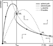
in the phase-plane diagram. As displayed in Figure 1, the isocline
is negatively sloped in the entire phase plane. This is because of
and F″(N; (1 − β)L)<0. Furthermore, as
,
is positive (negative) and depicted by upward (downward) pointed vertical arrows, in the region to the right (left) of this isocline. The slope of the isocline
is

as N [lEg ] N* and hence this isocline is displayed by an inverted U-shaped curve. Because
,
is negative (positive) and depicted by leftward (rightward) pointed horizontal arrows, in the region above (below) this isocline. The intersections of these isoclines and the directions of the horizontal and vertical arrows in their vicinity define two unstable steady states (in the positive quadrant)—an unstable focus SS1 and a saddle point SS2. As SS1 (SS2) is the steady state with a relatively high (low) control effort and hence a relatively low (high) number of users, it is not clear which of these steady states is DNI-superior. Although SS1 is supported by higher control cost, the drug-user intensive SS2 is associated with a greater loss of labor production capacity. As a marginal solution, SS0 at the origin also has to be considered.

Phase-plane diagram.
The depiction of SS1 and SS2 as an unstable focus point and a saddle point, respectively, bears a resemblance to the phase portrait in the unconstrained model of Tragler et al. (2001). The low control and large user number steady state SS2 has a stable manifold consisting of two arms. One arm leads to SS2 from North-West, indicating that it is optimal to gradually reduce control effort and allow the number of users to rise. The other arm converges to SS2 from South-East, revealing that it is optimal to gradually increase control effort and thereby reduce the number of users. By contrast, the path leading from North-East to SS0 also has to be considered as an optimal solution. This implies that it is optimal to increase the number of controllers at first and, falling below some number of users, the number of controllers can be reduced. From this kind of phase portrait, an unstable focus between two optimal long-run steady states, the existence of a DNS point can directly be concluded (see Feichtinger and Hartl 1986).9
The existence of a DNS point in the present framework is similar to the one in the special case described by Tragler et al. (2001) of unconstrained control budget and slowly diminishing returns on treatment, and to the critical point in the analogous case of efficient management of renewable natural resources with a convex-concave growth function in the state variable proposed by Clark (1971, 1976) and proven by Majumdar and Mitra (1980).
It is unlikely in reality for illicit drug use to be completely eliminated because as user numbers dwindle, it becomes increasingly difficult for officials to identify remaining users. It is also difficult to envisage government employing the control effort required for eliminating a problem that is yet to become apparent.
.
STEADY STATES AND THE EFFECTS OF THE MODEL PARAMETERS
To facilitate the analysis of the effects of the model parameters on the steady states, the diffusion function (F) is taken to be logistic:

with 0<α<1 indicating the intrinsic proliferation rate of drug use. In this case, the aforementioned no-arbitrage rule and the state-equation are displayed by the following system of nonlinear differential equations:


By substituting
into this system,

where Nss satisfies the following polynomial:

Consequently, the stationary level of gross national income (GNIss) is given by:

while the stationary disposable national income (DNIss) is given by:

A change in any of the model parameters affects the numbers of users and controllers and, consequently, the disposable national incomes in the steady states. From (17), DNISS decreases with both NSS and
and is affected, through NSS and
, by any model parameter γ with an elasticity that is a linear combination of the elasticities of control and use with respect to that parameter:

The directions of the effects of parameter changes on the steady states cannot be assessed by total differentiation of (14), (15), and (17) (see, for instance,
in Appendix C). Nevertheless, insights on the effects of a parameter change on the steady-state levels of the endogenous variables can be gained from the shifts of the isoclines
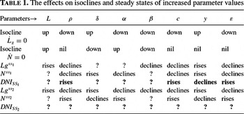
and
. Table 1 summarizes the effect of an increase in each parameter on the isoclines and thus on the high- and low-control steady-state levels of N, Lg, and, in recalling (17), disposable national income. The effects of all (some) of the model parameters on the low- (high-) control stationary levels of disposable national income are not clear because of opposing or unclear effects on the stationary numbers of users and controllers. The high-control stationary level of disposable national income rises, because of a decline in the numbers of users and controllers, with the planner's discount rate, with the gradient of the private and social marginal cost of control effort and with the relative productivity of users; but declines, because of an increase in control spending and in the number of users, with the full-potential personal income.

EXTENSIONS
Two extensions of the model are outlined in this section. The first extension distinguishes, as in Tragler et al. (2001), between two types of control activities—prevention and rehabilitation—and shows how their efficient levels of implementation depend on their relative effectiveness and cost. The second extension incorporates societal costs of disharmony between nonusers and users.
Efficient Mix of Rehabilitation and Prevention
The government's effort in controlling the number of users may take different modes that for simplicity we categorize as rehabilitation and prevention. As indicated in the Introduction, we define prevention as law enforcement and treatment activities that deter initiation, and rehabilitation as a process in which long-term dependent users are restored to a drug-free existence. The optimal investment of effort in rehabilitation and prevention depends on the effectiveness and social cost differentials between these activities. The convexity of the private and social costs of prevention and rehabilitation ensures the optimality of mixed effort as long as those differentials are not too high in favor of one of the activities.
Letting 0≤ϕ(t)≤1 be the proportion of Lg(t) invested in rehabilitation at t, then the user-nonuser conversion equation (2) and the control cost equation (3) are modified as follows:

where δr and δp are positive scalars denoting the marginal conversion and the marginal deterrent of the effort invested in rehabilitation and prevention, respectively; and where cr and cp are positive scalars denoting the coefficients of the private and social costs associated with investments of effort in rehabilitation and prevention, respectively.
It is possible that, because of its involuntary nature and its direct and external effects, prevention leads to higher levels of crime, violence, and drug-quality uncertainty than does an equal investment of effort in rehabilitation. In this case, rehabilitation generates lower personal and social costs than prevention for any equal level of effort cr<cp. Because of the convexity of the private and social costs, however, there exists a sequence of portfolios of drug-use control activities with 0<ϕ*(t)<1 for every t∈(0, ∞] that is growth-superior to investment in rehabilitation exclusively (ϕ(t)=1) even when, in addition to cr<cp, δr≥δp, as long as cp and δr are not enormously larger than cr and δp, respectively.11
See discussion of the relative effectiveness of prevention and rehabilitation in Gerstein, Johnson, Harwood, Fountain, Suter, and Malloy (1994), Rydell, Caulkins, and Everingham (1996), Caulkins, Rydell, Schwabe, and Chiese (1997), and Crane, Rivolo, and Comfort (1997).
As shown in Appendix D, the trajectory of the mixed effort that maximizes the sum of the disposable national incomes accruing over an infinite planning horizon is given by the differential equation:

In turn, the efficient rehabilitation effort share in steady state is:

Because
and NSS are endogenous, this expression alone can only be used for assessing the direct effects of the model parameters on ϕSS. In this respect, note the crucial roles of the difference between the discount rate and the stationary marginal drug-use diffusion and the difference between the marginal effectiveness of prevention and rehabilitation that lead to the following propositions.
If the discount rate is greater (smaller) than the stationary marginal drug-use diffusion then the direct effect of the prevention-rehabilitation marginal effectiveness differential (δp−δr) on ϕSS is negative (positive).
If the discount rate is greater than the stationary marginal diffusion of drug-use then the direct effect of the rehabilitation's private and social cost coefficient cr on ϕSS is positive, zero, or negative when δp−δr is greater than, equal to, or smaller than,
, respectively.
If δp is smaller than δr and the discount rate is smaller than the stationary marginal diffusion of drug-use, then the direct effect of cr on ϕSS is positive.
If δp is greater (smaller) than δr then the direct effect of the planner's rate of time preference on the stationary share of rehabilitation effort is positive (negative).
If δp is greater than δr and the discount rate is greater than the stationary marginal drug-use diffusion, then the direct effect of the prevention's private and social cost coefficient cp on ϕSS is positive.
If either (neither) δp is smaller than δr or (nor) the discount rate is smaller than the stationary marginal drug-use diffusion then the direct effect of personal full capacity output y on ϕSS is positive (negative).
If either (neither) δp is smaller than δr or (nor) the discount rate is smaller than the stationary marginal drug-use diffusion then the direct effect of the users' relative productivity ε on ϕSS is negative (positive).
If δp is smaller (greater) than δr and the stationary marginal drug-use diffusion increases with the size of the vulnerable labor force (1−β)L (as is the case when the diffusion function is logistic), then the direct effect of L on ϕSS is positive (negative), whereas the direct effect of the drug-use resistant population share β on ϕSS is negative (positive).
Finally, if δp=δr then ϕSS=cp/(cr+cp).
Societal Disharmony
If substance abuse is sufficiently widespread, tensions between users and nonusers might arise.12
In the case of AIDS, there exists tension between infected and noninfected people, and incidences of atrocities have been reported.
We assume that the relationship between costs of societal disharmony (CSDH) and the population share of users conforms to an inverted U-shaped curve.

CSDHmax is the maximum societal cost of disharmony that accrues when the population shares of users and nonusers are equal, and μ is a positive scalar reflecting the moderating effect of the quadratic distance from equal population shares on the cost of societal disharmony. This assumption implies, in conjunction with the assumptions made earlier, that the instantaneous DNI, now the gross national income net of the financial and social costs of prevention and the costs of societal disharmony, is given by:

Consequently, the efficient number of controllers is now:

subject to the motion equation (2). The no-arbitrage rule associated with this modification is (see details in Appendix E):

Because an extra infinitesimal effort in reducing the number of users does not necessarily reduce the level of societal disharmony,
as N(t)/L>reqqless0.5. If the number of users initially exceeds the number of nonusers, a rise in the control effort reduces the groups' size differential and thereby intensifies social tension. In this case, the efficient increase in control effort is smaller than would be the case were societal disharmony ignored. Conversely, if the number of nonusers initially exceeds the number of users, a rise in control effort increases the groups' size differential and hence reduces societal tension. In this case, the efficient increase in control effort is larger than would be the case were societal disharmony ignored.
SUMMARY AND CONCLUSIONS
In many countries, illicit drug use is a serious problem that reduces the number of fully productive workers and thereby aggregate output. This paper presents a dynamic control model—a hybrid of an epidemiological diffusion process and a macro economic objective—with a special reference to illicit drugs. The model is generic and also may be applicable to other hazardous substances, to epidemic control, and to socially undesirable activities such as crime.
The model divides the labor force into fully productive workers who do not use drugs and only partially productive users, and assumes that the use of drugs is contagious. In addition to foregone private output, costs are borne by government and society with the provision of control effort. Concerns about intra- and intergenerational diffusion of substance abuse motivates nonusers to bear part of the costs of the government control effort. Efficient management of the nation's portfolio of human resources is proposed as a path of drug-control effort that maximizes the present value of the stream of disposable national incomes. The efficient level of control varies during the planning horizon in accordance with the difference between the foregone gross national income stemming from an additional infinitesimal effort invested in control and the return, in terms of gross national income, on an additional unit of effort invested in that activity. The intertemporal change in control effort is moderated by the coefficient of the associated marginal personal and social costs. The foregone national income is taken as the product of the user cost of the typical controller and the marginal financial and social costs of the control effort. The user cost of a controller rises with the rate of time preference but is moderated by the instantaneous marginal “infection” of the labor force by users.
The steady states of the system comprising the derived equation of the efficient change in the control effort and the assumed proliferation equation are found to be an unstable focus with a high level of control and a low number of users and a saddle point with a low level of control and a high number of users. Below a critical number of users it is optimal, from an economic growth perspective, to eradicate drug use by applying a concerted initial control effort and then by gradually reducing control. Above that critical number of users it is optimal for the government to apply a much lower level of initial control and to gradually reduce control so that the economy converges to the steady state with low-control effort and a high number of users.
The effects of the model parameters on the high-control and low-control steady-state numbers of users and controllers, and subsequently on the steady state disposable national income, also were analyzed. The effects of each model parameter on the level of disposable national income in the low-control steady state are indeterminate. In the high-control steady state, disposable national income increases, because of a decline in the numbers of users and controllers, with the discount rate, with the gradient of the private and social marginal cost of control effort and with the relative productivity of users, but declines, because of increases in control spending and the number of users, with full-potential personal income.
The model was expanded to reflect on the composition of control effort. There are cost and benefit differences between rehabilitation and prevention. As long as these differences are not too high in favor of one of the activities, convexity of the private and social costs of prevention and rehabilitation ensures the optimality of mixed effort. The propositions concerning the direct effects of drug control's benefit and cost coefficients, the personal full capacity output and the users' relative productivity on the stationary rehabilitation-prevention mix reflected the crucial roles of the difference between the marginal effectiveness of prevention and rehabilitation and the difference between the discount rate and the stationary marginal diffusion of drug use.
The model also was expanded to incorporate tension between users and nonusers. It was shown that if the number of users initially exceeds the number of nonusers, raising the control effort diminishes the groups' size differential and, in turn, intensifies societal tension. In this case, the efficient rise in control effort is smaller than would be the case were societal tension ignored. Conversely, when initially the number of nonusers exceeds the number of users, raising the control effort increases the groups' size differential and subsequently reduces the level of societal tension. In this case, the efficient rise in control effort is larger than would be the case were societal disharmony ignored.
APPENDIX A
THE NECESSARY CONDITIONS AND THE NO-ARBITRAGE RULE
The (present value) Hamiltonian associated with (5) and (2) is

The necessary conditions for maximum are:

(2) and the transversality condition
.
(6) is obtained by dividing both sides of (A2) by λ and considering that by virtue of (A3) λ(t)=−eρt[y+2cLg(t)]/δ. The no-arbitrage rule (7) is obtained by differentiating the optimality condition (A3) with respect to t (singular control), substituting the information contained in conditions (A2) and (A3) for
and λ, respectively, multiplying both sides by eρt/2c and rearranging terms. It also can be obtained by using Euler equation.
APPENDIX B
THE NECESSARY CONDITIONS FOR THE STATE CONSTRAINT N(t)≥0
Considering (A1), the Lagrangian Λ(t) for the state constraint N(t)≥0 becomes

Following Kamien and Schwartz (1991, p. 230), the necessary optimality conditions are:

Therefore, the constrained canonical system is:


Furthermore, as the Legendre-Clebsh condition
is satisfied it is assured that the costate λ(t) and control Lg(t) are continuous at switching points where the state constraint becomes active (see, for example, Feichtinger and Hartl, 1986). From (B6) it can be seen that the origin in the state control space is a candidate for an optimal solution. To prove (B4) we get from (B2), Lg=0 and because of the continuity of the costate variable at the switching time t0:

Setting now
and substituting (B8) the following equality for ν(t) with t≥t0 holds.

As ε<1, F′(N(t); (1−β)L)>0, y>0 and δ>0 have been assumed, this proves ν(t)>0 for t≥t0. Hence, N=0=Lg satisfies the necessary optimality conditions.
APPENDIX C
THE EFFECTS OF CHANGES IN THE MODEL PARAMETERS
The effects of changes in L, ρ, δ, α, β, c, y, and ε on Nss are as follows:


APPENDIX D
THE NO-ARBITRAGE RULE OF EQUATION (21)
The decision problem in Section 6 is:

subject to the state equation (19) and N(∞)≥0. The Hamiltonian associated with this problem is

The necessary conditions for maximum are


(21) is obtained by dividing both side of (D4) by Lg, differentiating with respect to t, substituting the right-hand side of (D3) for
and the expression of λ from (D4), and rearranging terms.
APPENDIX E
THE NO-ARBITRAGE RULE OF EQUATION (26)
The Hamiltonian associated with this decision problem is

The necessary conditions for maximum are


(2) and the transversality condition
. The no-arbitrage rule (26) is obtained by differentiating the optimality condition (E3) with respect to t (singular control), substituting the information contained in conditions (E2) and (E3) for
and λ, respectively, multiplying both sides by eρt/C″(Lg(t)) and rearranging terms.