1 Introduction
The application of periodic excitations to a fluid system with a density gradient can lead to a wide variety of patterns and complex dynamics (Wolf Reference Wolf1970; Talib, Jalikop & Juel Reference Talib, Jalikop and Juel2007; Benilov & Chugunova Reference Benilov and Chugunova2010; Shevtsova et al. Reference Shevtsova, Ryzhkov, Melnikov, Gaponenko and Mialdun2010; Borcia, Borcia & Bestehorn Reference Borcia, Borcia and Bestehorn2014; Tinao et al. Reference Tinao, Porter, Laverón-Simavilla and Fernández2014; Shevtsova et al. Reference Shevtsova, Gaponenko, Yasnou, Mialdun and Nepomnyashchy2015a ). In spite of the substantial advances in the study of Faraday waves and Kelvin–Helmholtz types of instability, their simultaneous existence in the same system has not been reported so far. Due to different phenomena involved, the effects of normal and tangential vibrations are usually considered separately: the former affects the interface by changing the effective gravity and, thus, the hydrostatic pressure gradient, whereas the latter induces a shear flow in containers with side walls.
Vertical periodic acceleration of fluid layers (parallel to the density gradient) with amplitude
 $A$
and angular frequency
 ${\it\omega}=2{\rm\pi}f$
induces patterns of standing waves on the interface with a frequency
 $f/2$
that is one-half of the forcing frequency
 $f$
(Benjamin & Ursell Reference Benjamin and Ursell1954; Kumar & Tuckerman Reference Kumar and Tuckerman1994; Diwakar et al.
Reference Diwakar, Zoueshtiagh, Amiroudine and Narayanan2015). This phenomenon is called Faraday instability.
The behaviour of an interface of immiscible liquids under horizontal vibrations in a container with end walls demonstrates the emergence of spatially periodic waves on the interface, which are often referred to as ‘frozen waves’ (Lyubimov & Cherepanov Reference Lyubimov and Cherepanov1987; Khenner et al. Reference Khenner, Lyubimov, Belozerova and Roux1999; Ivanova, Kozlov & Evesque Reference Ivanova, Kozlov and Evesque2001; Jalikop & Juel Reference Jalikop and Juel2009; Gandikota et al. Reference Gandikota, Chatain, Amiroudine, Lyubimova and Beysens2014). The frozen waves are caused by a shear driven mechanism similar to the Kelvin–Helmholtz instability. The distinction is that, as a result of a harmonic change in the flow direction, the wave remains on average in the same place, as its profile is frozen in the reference frame of a vibrating container.
Recent experiments (Gaponenko et al.
Reference Gaponenko, Torregrosa, Yasnou, Mialdun and Shevtsova2015a
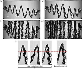
) presented evidence that an interfacial instability also exists between two miscible liquids of similar (but non-identical) viscosities and densities. One of the features that highlights the difference between immiscible and miscible fluids under horizontal vibrations is the shape of the frozen waves. In the former case, the waves have a sinusoidal shape while in the latter case, a saw-tooth frozen structure is formed above the threshold instability in a gravity field. In microgravity in the case of immiscible liquids, the surface tension will be dominant. In the case of miscible liquids in microgravity, the mechanisms that limit the growth of amplitude (gravity and effective interfacial tension) vanish but the mechanisms that initially drove the instability (density gradient and inertia) become weak with time. This leads to a fascinating interfacial pattern which presents a series of vertical columns of alternating liquids (Gaponenko et al.
Reference Gaponenko, Torregrosa, Yasnou, Mialdun and Shevtsova2015b
). After the formation of waves on the miscible interface, they grow without saturating until the interface reaches the upper and lower walls. The final enduring flow pattern consists of a series of vertical columns of alternating liquids, which occupy the whole height of the cell similar to that shown in figure 5 at
 $t=4.1$
s.
In this study, we provide evidence that the periodic wave pattern created by the Kelvin–Helmholtz type of instability gives birth to Faraday waves in both cases of reduced and normal gravity.
2 Experiments
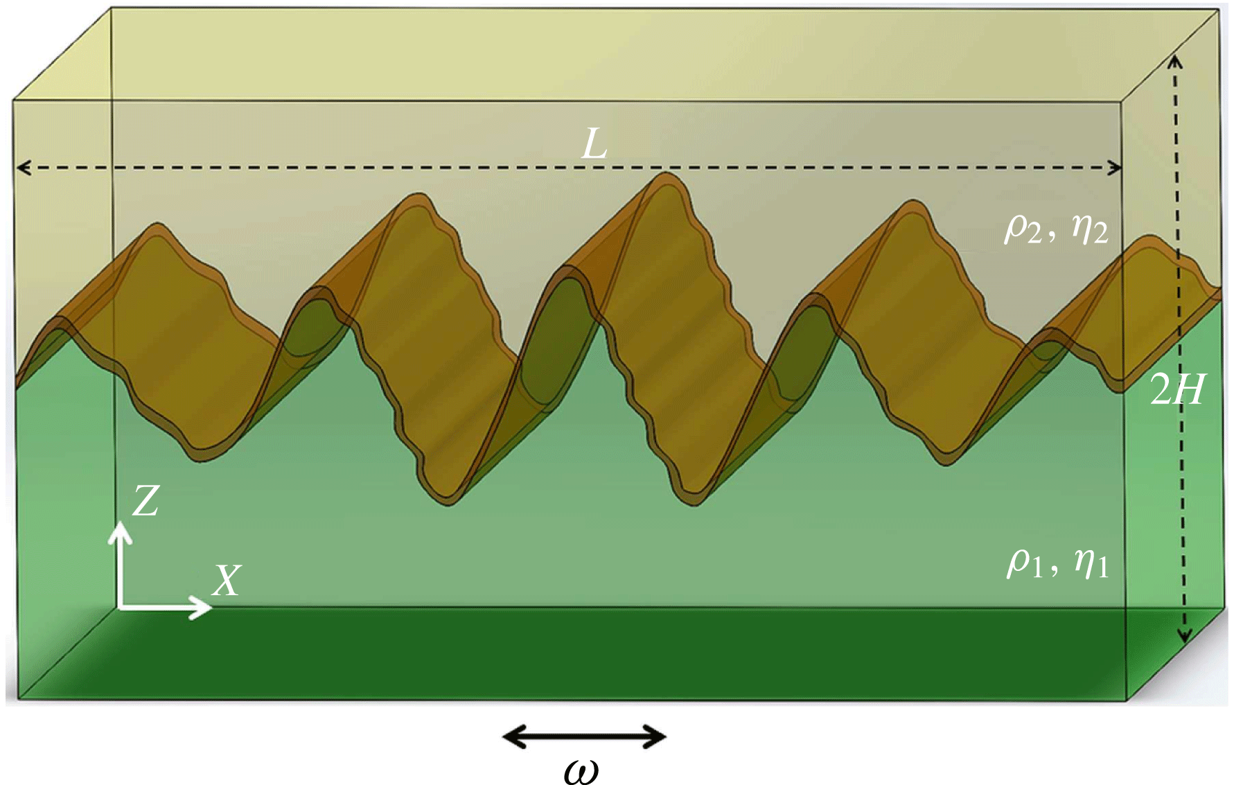
To gain an insight into these issues, we consider two layers of binary mixtures of the same constituents (water–alcohol mixtures of different percentage). The experiments were performed during normal gravity and microgravity under the conditions of a parabolic flight. The test cell sketched in figure 1 is attached to a linear motor, which performs translational oscillations in the
 $X$
direction at a controlled frequency and amplitude. The amplitude and frequency of vibrations were controlled by position versus time records taken from the optical encoder of the linear motor. For each experimental run both the amplitude and frequency set by driving software were verified and validated against the actual values extracted from the encoder records. Since the resolution of the encoder is
 $5~{\rm\mu}\text{m}$
, we can estimate the uncertainty of the vibration amplitude as 0.3 % in the worst case. The linear motor is mechanically based on a single-axis bearing positioning stage, which by specification has a maximum off-axis displacement of
 $25~{\rm\mu}\text{m}/300~\text{mm}$
. These data provide the angular uncertainty in the direction of the vibrations as
 $0.01^{\circ }$
. To isolate the effect of vibrations on the environment a special anti-vibration cork/elastomer pad of 12.5 mm thickness has been mounted in between the linear motor and the rack structure.
The scheme of a test cell. The test cell is a cavity of
 $L\times 2H\times W=15~\text{mm}\times 7.5~\text{mm}\times 5~\text{mm}$
. The layers have equal thicknesses
 $H$
. The fluids used were a 90 % (mass) solution of water in isopropanol and a 50 % (mass) solution of water in isopropanol. The density and viscosity contrasts between the two fluids are
 ${\it\rho}={\it\rho}_{2}/{\it\rho}_{1}=0.92$
,
 ${\it\eta}={\it\eta}_{2}/{\it\eta}_{1}=2.17$
, see table 1.

The net acceleration applied to the system is the sum of the gravitational
 $\boldsymbol{g}$
and vibrational
 $\boldsymbol{g}_{os}=A{\it\omega}^{2}\boldsymbol{e}$
accelerations (
 ${\it\omega}=2{\rm\pi}f$
), i.e.
 $$\begin{eqnarray}\boldsymbol{g}(t)+\boldsymbol{g}_{os}\cos ({\it\omega}t),\quad \boldsymbol{g}(t)=(g_{X},g_{Y},g_{Z}).\end{eqnarray}$$
In the experiments, the frequency and amplitude were varied within the ranges 2–24 Hz and 1.5–16 mm, respectively. The two opposite side walls of the cell are transparent and the flow dynamics was monitored by direct shadowgraphy of the interface. Deviation of the light path due to the high density gradient results in images with dark regions corresponding to the interface. The camera was fixed to the linear motor. A typical data set consisted of 600 images taken at 48 f.p.s. and covering 12.5 s in time, but sometimes we used an acquisition of 24 f.p.s. for observation during the whole period of microgravity. More details on the experimental technique can be found in the recent publication by Gaponenko et al. (Reference Gaponenko, Torregrosa, Yasnou, Mialdun and Shevtsova2015a ).
The interface is considered in the thermodynamic sense (Vorobev Reference Vorobev2014) and represented as a transient layer of small but non-zero thickness. We have performed a special study to estimate its thickness because it was reported (Zoueshtiagh, Amiroudine & Narayanan Reference Zoueshtiagh, Amiroudine and Narayanan2009) that the thickness of the diffusion layer at a miscible interface is an important parameter in the Faraday instability. The accuracy of the shadowgraphy does not allow such a study and, for this reason, a Mach–Zehnder interferometer was used. This set-up was built for the measurement of diffusion coefficients (Mialdun et al.
Reference Mialdun, Sechenyh, Legros, Ortiz de Zárate and Shevtsova2013a
; Mialdun, Yasnou & Shevtsova Reference Mialdun, Yasnou and Shevtsova2013b
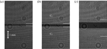
). A large concentration difference between the two liquids produces a strong change in the refractive index at the interfacial region and this leads to a strong beam deflection, converting the interface location into a black strip (see figure 2). The interferometer was aligned to produce a vertical narrow fringe pattern in the regions with uniform concentration, as seen at
 $t=0$
in figure 2. The fringes start bending and deviating from the vertical in the region where the concentration changes. On the basis of these deviations, the white dashed lines were drawn in figure 2 which indicate the thickness of the diffusive interface at representative time moments: (a) injection is stopped,
 $t=0$
; (b) duration of the microgravity time,
 $t=20$
s and (c)
 $t=300$
s (for reference). An accurate inspection of the initial interface at
 $t=0$
gives a thickness of
 $0.3~\text{mm}$
. In the pure diffusive regime presented in figure 2, the interface thickness attains 0.6 mm during 20 s (the longest experimental time), but still it can be considered as sharp. As a rule, experiments started a few seconds after injection and in the numerical simulations the interface thickness,
 $h=0.45$
mm, was utilized. The last image demonstrates that at
 $t=300$
s the mixing layer propagates to almost half of the bottom layer. It is interesting to note that this propagation is non-symmetric, because the mass diffusion coefficient in the lower liquid is five times larger than in the upper layer. The physical properties of the mixtures and the useful parameters are listed in table 1.
Thickness of the interface between solutions of water–isopropanol with water concentration
 $C_{1}=0.90$
mass fr. (bottom) and
 $C_{2}=0.50$
mass fr. (top) analysed by interferometry. The cropped central part of the cell of
 $4~\text{mm}\times 7~\text{mm}$
size is shown. Injection rate is
 $0.80~\text{ml}~\text{min}^{-1}$
which is typical for the all experiments. (a)
 $t=0$
s, time instant when an injection is stopped; (b)
 $t=20$
s, typical duration of the microgravity time, and (c)
 $t=300$
s.

The physical properties of the mixtures 90 % water–10 % IPA and 50 % water–50 % IPA (mass fraction) at
 $25\,^{\circ }\text{C}$
: density
 ${\it\rho}$
, kinematic viscosity
 ${\it\eta}$
, diffusion coefficient
 $D$
, the thickness of vibrational viscous boundary layers in the experimental parameter space
 ${\it\delta}=\sqrt{2{\it\nu}/{\it\omega}}$
, the diffusion time (
 ${\it\tau}_{D}^{\ast }=h^{2}/D$
) over the initial interface thickness
 $h=0.45\times 10^{-3}$
m.

Parabolic flights provided repeated periods of approximately 20 s of reduced gravity preceded and followed by 20 s of hypergravity (up to
 $1.8g_{0}$
), and then normal gravity
 $g\sim 1g_{0}$
, where
 $g_{0}=-9.81~\text{m}~\text{s}^{-2}$
. The microgravity level during the parabolas was
 $|g_{X,Y}/g_{0}|\leqslant 0.01$
,
 $|g_{Z}/g_{0}|\leqslant 0.05$
. Because of the irreversibility of the mixing process, each experiment with miscible liquids required a fresh refill of the cell. The ground-based experiments were also conducted inside an airplane when the set-up was firmly fixed to its body.
3 Results and discussion
3.1 Observation in microgravity
In the present study we consider the cases when the amplitude of excitations is large,
 $A\geqslant 2H$
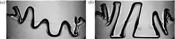
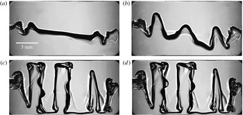
. Figure 3 presents the dynamics of the interface below the threshold of secondary instability for reference. The amplitude of the interfacial waves grows with time and the wavy pattern transforms into a series of vertical columns of alternating liquids. The case above the threshold is shown in figure 4 for the same excitation amplitude and a higher frequency. The first two snapshots illustrate that above the critical excitation of the secondary instability, in the beginning, a wavy pattern develops similarly. As soon as the height of the interfacial waves becomes large enough (the crest-to-trough length is approximately one-half of the thickness of the layer), the secondary instability is evoked in the system in the form of standing waves over frozen waves. These small-scale waves can be seen on the right sides of the columns in the snapshots at
 $t=2.9$
s and
 $t=3.025$
s in figure 4. These snapshots are shifted in time by one oscillation period and it can be seen that the secondary waves on the central column are at the opposite phase of oscillations.
The evolution of an interfacial instability in a microgravity experiment below the threshold of the Faraday instability. The cell with miscible liquids is vibrated horizontally at
 $f=6$
Hz,
 $A=10.4$
mm at
 $t=1.7$
s (a), 3.14 s (b).

A time sequence of images from a microgravity experiment presenting the evolution of a flow pattern in the cell with miscible liquids vibrating horizontally at
 $f=8$
Hz,
 $A=10.7$
mm at
 $t=1.4$
s (a), 1.8 s (b). The Faraday waves on the columns are seen at
 $t=2.9$
s (c) and 3.025 s (d). The two snapshots at the bottom are shifted in time by one oscillation period,
 $T=0.125$
s.

Since the secondary instability generates standing waves which oscillate at one-half of the driving frequency, it presents classical Faraday waves. A close inspection of another experiment in figure 5 supports these observations. In the case of a larger oscillation frequency the standing waves are already visible at
 $t=1.5$
s in the thickest part of the triangles, they are pointed out in figure 5 by the white circles. The waves appear at the troughs of the triangles and rapidly cover the whole length of the saw-tooth structure (snapshots at
 $t=1.75$
s in panels (a,b)). The temporal behaviour of the central peak is shown in figure 5(e) for more detailed examination. The red line helps to follow the interface distortion. The first three snapshots display the evolution of the pattern over one oscillation period of the external excitation. At the end of the period,
 $T=1/f_{0}$
, the wave is in the opposite phase with respect to the initial state, and only at the end of the second period does it return to the same phase (the last snapshot). This confirms that the frequency of the standing wave is one-half of the external frequency
 $f_{0}/2$
, which is the signature of the classic Faraday wave instability. A more detailed time evolution is presented in the supplementary movie available online at http://dx.doi.org/10.1017/jfm.2016.222 (VIPIL-PF).
Microgravity experiment when
 $f=16$
Hz,
 $A=6.7$
mm. The development of the Faraday waves (secondary instability) over the growing frozen structures: (
 $t=1.5$
s (a)) the appearance of the Faraday waves; (
 $t=1.75$
s (b)) the Faraday waves occur alternately on one or other side of the growing triangle; (
 $t=2.8$
s (c)) intense time-dependent wave motion over the entire column interface; (
 $t=4.1$
s (d)) the disappearance of the Faraday waves. Panel (e) presents only the central peak from the image at
 $t=1.75$
s at different phases of oscillations proving a subharmonic frequency in the interface motion.

Figures 4 and 5 show that, depending on the oscillation phase, the standing wave appears on the left or right side of the triangle. Later, at
 $t=2.8$
s, the waves occur on both sides of the columns. In course of time a transient layer mimicking the interface widens due to mixing on a small scale and the Faraday waves disappear. Observing these fascinating images, we would like to note that the liquids are miscible at any proportion (water and alcohol of different concentrations).
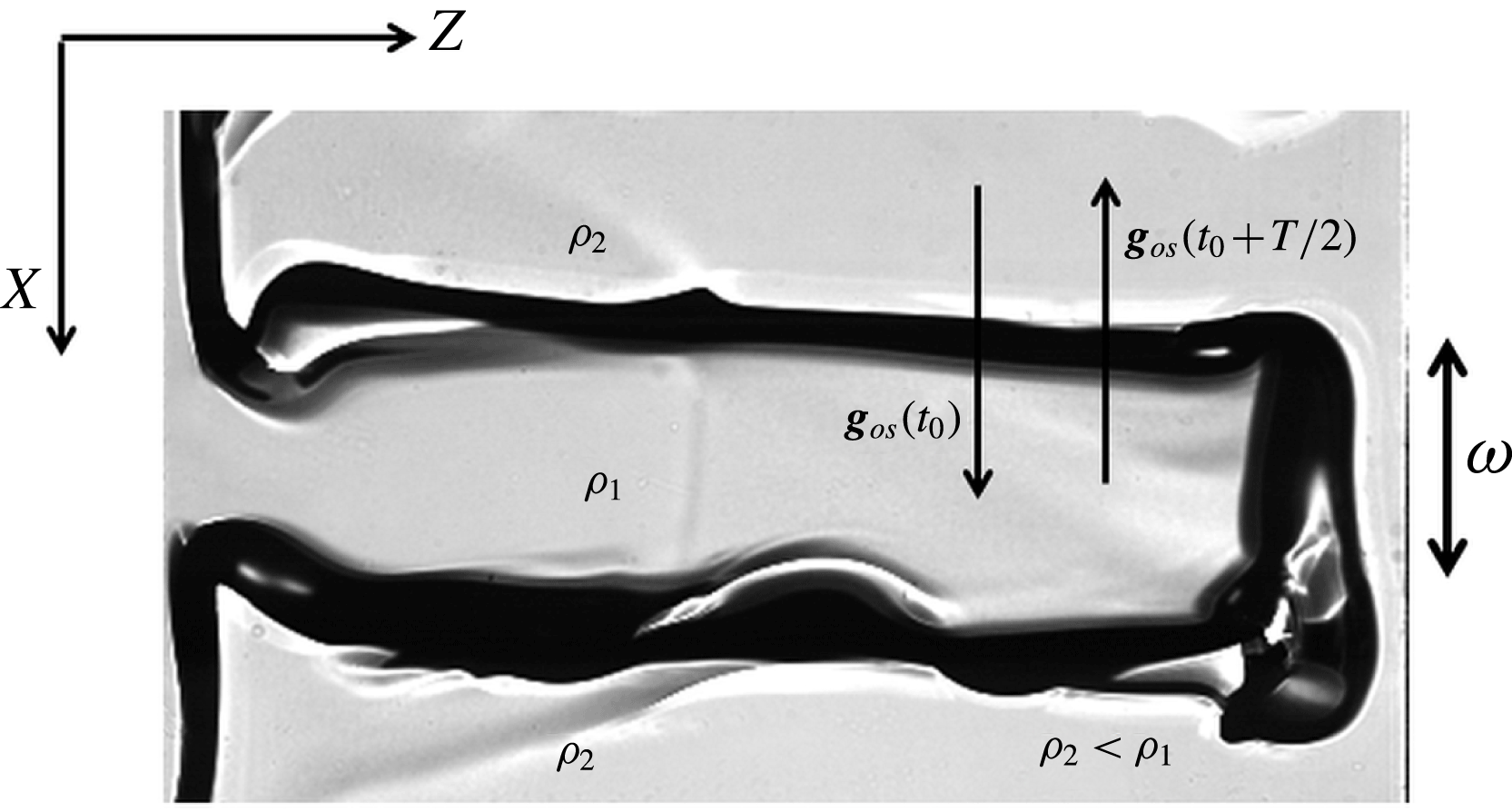
In order to explain these observations, in figure 6 one of the columns is placed horizontally. In microgravity experiments, steady (residual) gravity in the direction perpendicular to the lateral interface of the columns is absent (
 $|g_{X}|<0.01g_{0}$
). Due to the sign change of vibrational acceleration, the system spends half of the period in the regions of effective negative acceleration. Consequently, the interface becomes unstable due to the Rayleigh–Taylor type of instability when a heavier fluid is over a lighter one, which occurs on one of the lateral interfaces of the column. Here, it is enough to have different densities. On the other side of the column the situation will be the same when acceleration switches sign, as the ratio of densities will then be the inverse. Thus, we present experimental evidence of the agreement between the Rayleigh–Taylor and Faraday instabilities which was theoretically predicted by Kumar (Reference Kumar2000) in deep layers (wavelength
 $\ll$
liquid depth).
Schematic of Faraday wave development on one side of the column in the system when effective gravity switches sign. For explanation the central column in figure 4 (image at
 $t=2.9$
s) is turned by
 ${\rm\pi}/2$
.

The determination of the wavelength is ambiguous even for the columnar structure, since the width of the columns varies along the container. Furthermore, the system behaviour is highly transient. For the frozen waves we may introduce the wavelength
 ${\it\lambda}_{fr}$
measured as the double width of the largest column while it reaches both walls, i.e. the central column at
 $t=2.9$
s in figure 4 or at
 $t=2.8$
s in figure 5. Using this plausible assumption, we postulate that the wavelength of the Faraday wave
 ${\it\lambda}_{FW}$
is approximately two times smaller than that of frozen waves. Consequently, for
 $f=8$
Hz,
 $A=10.7$
mm (figure 4) the wavelength of the subharmonic wave is
 ${\it\lambda}_{FW}\approx 2.7$
mm and for
 $f=16$
Hz,
 $A=6.7$
mm (figure 5) it is
 ${\it\lambda}_{FW}\approx 1.7$
mm with an uncertainty of approximately 5–7 % based on human error. The dependence of
 ${\it\lambda}_{fr}$
upon the vibrational velocity
 $V_{os}=A{\it\omega}$
was discussed previously (Gaponenko et al.
Reference Gaponenko, Torregrosa, Yasnou, Mialdun and Shevtsova2015b
).
Figures 4 and 5 show two different regimes that track the evolution of Faraday waves depending on the strength of external forcing: for the weaker forcing,
 $g_{os}/g_{0}=2.75$
, the subharmonic pattern occurs on established columns (figure 4) while for the stronger forcing,
 $g_{os}/g_{0}=6.90$
, they begin to develop on the triangle structure (figure 5).
3.2 Observation under normal gravity
The existence of the instability of Kelvin–Helmholtz type between two miscible liquids subjected to horizontal vibrations under normal gravity has been recently evidenced experimentally and confirmed numerically by Gaponenko et al. (Reference Gaponenko, Torregrosa, Yasnou, Mialdun and Shevtsova2015a
). Unlike the microgravity case, in the Earth’s gravity the height of the frozen waves is stabilized and they do not reach the horizontal walls. As a general trend, the final saturated height of the frozen waves increases with vibrational velocity,
 $V_{os}=A{\it\omega}$
. Due to the limitation of our set-up, which concerns large frequencies, the Faraday waves were examined at large amplitudes.
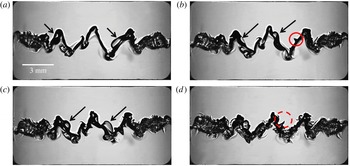
The formation, development and decay of frozen waves under normal gravity are much faster than under reduced gravity. As a result, the secondary instability develops and undergoes a small-scale breakdown within only a few oscillation periods. The development of subharmonic waves in the background of the frozen waves is clearly seen in figure 7 despite the intricate structure of interfacial patterns. Figure 7 also demonstrates that these small-amplitude waves are associated with a standing wave pattern. In particular, snapshots (b) at
 $t_{0}$
and (c) at
 $(t_{0}+T)$
show that the maximum and minimum of the wave exchange places over one period of vibration
 $T$
while the nodal point remains in the same place. Notice that at
 $t_{0}=0.65$
s, this means that the secondary instability is fully developed in six oscillation periods after the imposition of vibrations. As the camera acquisition rate (48 f.p.s.) is not an integer multiple of an imposed vibration frequency (10 Hz), it is not possible to show a more detailed wave evolution.
(Ground-based experiment) the existence of Faraday waves over frozen waves when
 $f=10$
Hz,
 $A=16.0$
mm (a)
 $t_{0}-T/2$
, (b)
 $t_{0}$
, (c)
 $t_{0}+T$
, (d)
 $t_{0}+2T$
. The snapshots (a,b) illustrate the interfacial pattern at different phases of the vibration period. The arrows focus attention on the largest amplitudes of Faraday waves;
 $t_{0}=0.65$
s,
 $T=1/f$
. The red circles draw attention to the occurrence of spikes on the interface.

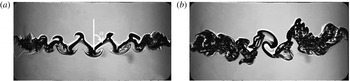
To highlight the existence of subharmonic waves in ground-based experiments, figure 8 shows two cases when the forcing is below and well above the critical forcing. Panel (a) corresponds to the amplitude below the critical excitation, while the frequency is the same as in figure 7. The frozen waves display a smooth triangle shape even at much later times than those when the subharmonic oscillations were observed in the previous case. The angle (
 ${\it\alpha}$
) between the interface and the vertical direction slightly depends on vibrational parameters and for current experiments it lies in a range between
 $0.15{\rm\pi}$
and
 $0.20{\rm\pi}$
. The side walls cause amplitude modulation of the saw-tooth pattern and, furthermore, they generate a fish spine pattern noticeable in the vicinity of the walls; the origin of this pattern was discussed previously (Shevtsova et al.
Reference Shevtsova, Gaponenko, Yasnou, Mialdun and Nepomnyashchy2015a
).
(Ground-based experiment) the snapshots illustrate interfacial pattern (a) below (
 $f=10$
Hz,
 $A=11.2$
mm),
 $t=1.64$
s; and (b) well above (
 $f=12$
Hz,
 $A=14.0$
mm),
 $t=0.8$
s; the threshold of the Faraday instability. The angle
 ${\it\alpha}$
of a frozen wave is measured between the vertical upward position and the interface position under vibrations.

At a very strong forcing the instability progresses more quickly, as indicated by the developed primarily and secondary patterns at time instant
 $t=0$
.8 s in figure 8(b). Another comment is that the amplitude of the subharmonic waves strongly increases and the system enters into a highly nonlinear regime. Note that in all ground-based experiments
 $A{\it\omega}^{2}>|g_{0}|$
and the effective gravity switches sign: i.e.
 $g_{os}/g_{0}=6.4$
, 4.5 and 8.1 in figures 7, 8(a) and 8(b), respectively. In line with the microgravity observations, the Faraday waves appear alternatively on each side of the triangle.
The peculiar feature of the secondary instability evidently observed in ground-based experiments is the formation of spikes on the interface. The Faraday wave gently sloshes the triangle interface during each period of oscillations. The interface is slightly deformed and it retains the trace of the wave. The new coming wave interacts with the trace left by the previous wave and forms a spike. A few examples are highlighted by the red circles in figure 7(b,d). With the strengthening of the Faraday waves, the spikes are created faster and, finally, the mixing layer widens and the saw-tooth interface becomes fuzzy, as can be seen in figure 7(d). The spikes have been observed in microgravity experiments as well, e.g. they are visible on the images in figure 5(e), but they develop at a later time and affect the shape of the interface more slowly. The formation of spikes seems to play an important role in the disappearance of the Faraday waves for both types of experiments, i.e. in normal and reduced gravity. The interface of the columns shown in figure 5 in the snapshot at
 $t=4.1$
s is covered by the spikes.
3.3 Numerical simulations
Numerical simulations of nonlinear Navier–Stokes and mass conservation equations have been performed in order to confirm experimental observations and predict the evolution of the system for parameters out of the experimental area. Because both layers are composed of the same liquids (water–isopropanol), it allows us to consider a one-layer system with a sharp change in concentration at
 $Z=H$
at the initial step. The relative concentration of the denser liquid (water), normalized by the initial concentration difference of water between layers, is selected as an independent variable
 $C$
, i.e. at the initial moment
 $C=1$
in the lower liquid while
 $C=0$
in the upper one. The linear transition of the concentration is considered inside the region of 0.45 mm between the layers. The densities, viscosities, cell dimensions correspond to the experimental values listed in table 1 and into the legend to figure 1. The numerical approach is similar to that used in recent publications (Gaponenko et al.
Reference Gaponenko, Torregrosa, Yasnou, Mialdun and Shevtsova2015a
; Shevtsova et al.
Reference Shevtsova, Gaponenko, Sechenyh, Melnikov, Lyubimova and Mialdun2015b
).
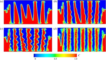
Figure 9 presents several sets of calculations at
 $g=0$
where experiments are not accessible, i.e. at high frequencies when changing the amplitude. As a general tendency (with a few deviations), the number of columns increases with the increase of the amplitude at a fixed
 $f$
and reaches the limit number prior to the secondary instability. The observations of the interfacial patterns below and above the threshold in figure 9 support this statement. A further increase of the forcing-amplitude results in the amplification of the Faraday waves at the same number of columns (figure 9
c) and, finally, in formation of a thick mixing layer (figure 9
d) over the column. The important finding about the number of constant columns suggests that the Faraday instability refrains further development of frozen wave instability.
Numerical interfacial patterns shown as the concentration fields below (a) and above (b,c) the threshold of Faraday waves in microgravity at
 $t=1$
s. The frequency is the same in all patterns
 $f=20$
Hz but the amplitudes are different: (a)
 $A=5.0$
mm; (b)
 $A=6.0$
mm; (c,d)
 $A=6.5$
mm. Panel (d) shows the pattern (c) at later time,
 $t=3$
s.

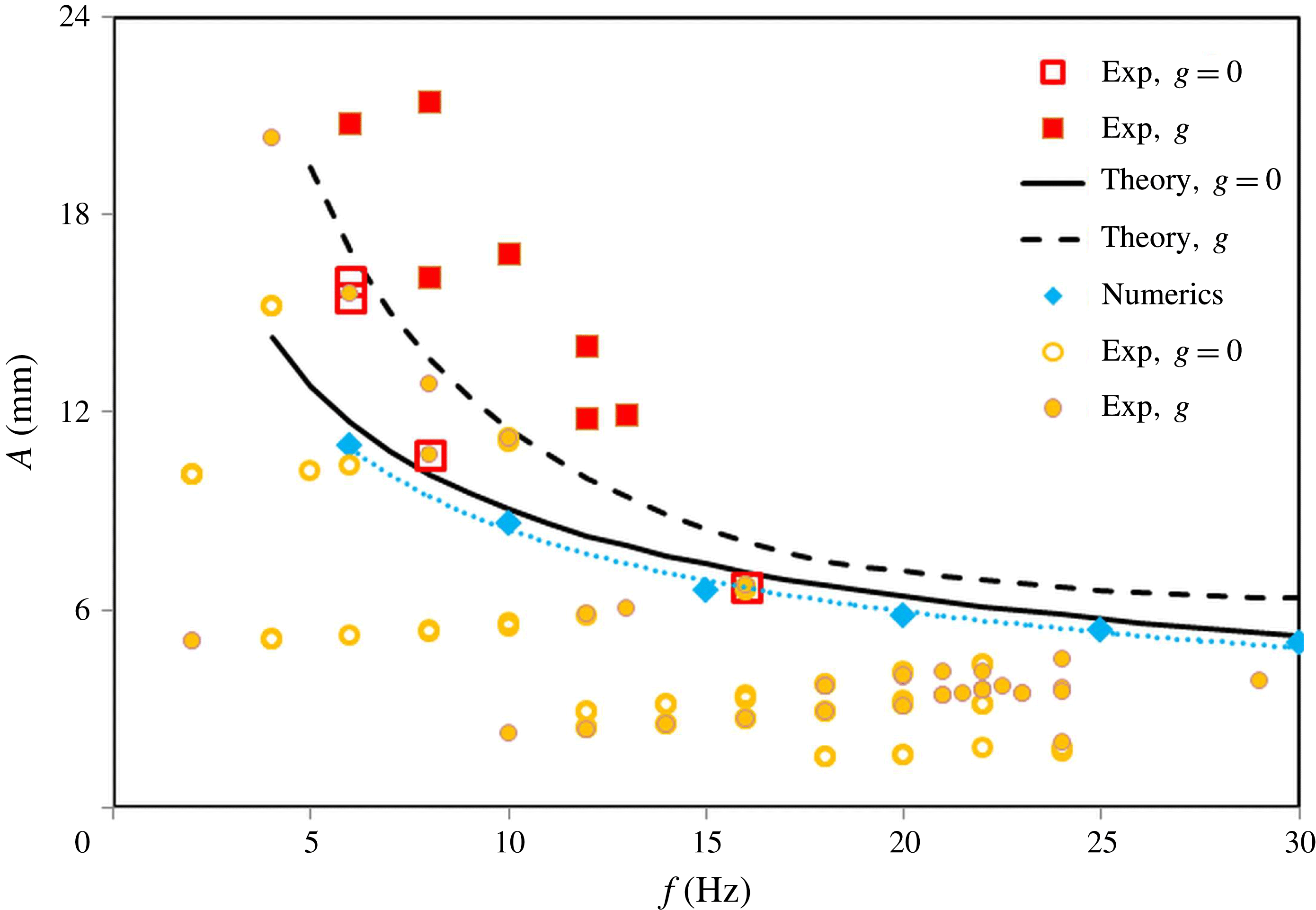
In line with the experimental findings, the numerical results have confirmed that two-scale patterns, which consist of both frozen and Faraday waves, occur at a miscible interface with zero surface tension and in the absence of gravity. Furthermore, the results of computer simulations well reproduce the experimental observations in terms of the existence, shape and development of subharmonic waves. The results of the simulations quantitatively characterize the response of the interface to the vibrational forcing; the threshold of the standing waves is shown by a dotted curve and rhombi in figure 10.
Stability map for emergence of the Faraday waves on the background of frozen structures. The points at which subharmonic waves were observed in the experiments are shown by open (
 $g=0$
) and filled (
 $g\neq 0$
) squares. The points at which Faraday waves were not observed are shown by open (
 $g=0$
) and filled (
 $g\neq 0$
) circles. The instability thresholds obtained by the theory are shown by solid (
 $g=0$
) and dashed (
 $g\neq 0$
) curves. The numerical threshold (
 $g=0$
) is shown by rhombi and a dotted trend curve.

3.4 Theoretical estimates for the threshold of Faraday waves
To justify the suggestion that the instability studied experimentally and numerically in the previous sections is indeed the Faraday instability, we present here a simple theoretical estimate of the critical amplitude based on the damped Mathieu equation for the waves on the boundary between two media with different densities,
 $$\begin{eqnarray}\text{d}^{2}{\it\zeta}/\text{d}t^{2}+2{\it\gamma}(k)\,\text{d}{\it\zeta}/\text{d}t+F(k,t){\it\zeta}=0,\end{eqnarray}$$
derived by Kumar & Tuckerman (Reference Kumar and Tuckerman1994) under conditions of weak forcing and weak damping. Here
 $k$
is the wavenumber of the Faraday wave,
 $$\begin{eqnarray}\displaystyle F(k,t)=g_{eff}(t)k({\it\rho}_{1}-{\it\rho}_{2})/({\it\rho}_{1}+{\it\rho}_{2}), & & \displaystyle\end{eqnarray}$$
 $$\begin{eqnarray}\displaystyle g_{eff}(t)=g_{0}+g_{os}\cos {\it\omega}t,\quad {\it\gamma}(k)=2k^{2}\frac{{\it\eta}_{1}+{\it\eta}_{2}}{{\it\rho}_{1}+{\it\rho}_{2}}. & & \displaystyle\end{eqnarray}$$
In order to obtain analytical expressions that describe the functional dependence of the critical amplitude
 $A$
on the relevant physical parameters, we approximate the solution corresponding to the subharmonic stability boundary by just two Fourier components,
 ${\it\zeta}={\it\zeta}_{+}\exp (\text{i}{\it\omega}t/2)+{\it\zeta}_{-}\exp (-\text{i}{\it\omega}t/2)$
.
Note that the self-consistent theory of Faraday instability in a viscous liquid is based on a coupled system of equations that include an equation for the surface deformation and a boundary value problem for the vertical velocities in both liquids (see Besson, Edwards & Tuckerman Reference Besson, Edwards and Tuckerman1996). We assume however that the application of a rigorous theory would change the numerical values but not the qualitative dependence of the instability threshold on the parameters.
In the framework of the approximation described above, we obtain the following simplified expression for the instability threshold,
 $$\begin{eqnarray}\displaystyle \frac{g_{os}^{2}k^{2}}{4}\left(\frac{{\it\rho}_{1}-{\it\rho}_{2}}{{\it\rho}_{1}+{\it\rho}_{2}}\right)^{2}=\left[\frac{{\it\omega}^{2}}{4}-\frac{g_{0}\,k({\it\rho}_{1}-{\it\rho}_{2})}{{\it\rho}_{1}+{\it\rho}_{2}}\right]^{2}+4{\it\omega}^{2}k^{4}\left(\frac{{\it\eta}_{1}+{\it\eta}_{2}}{{\it\rho}_{1}+{\it\rho}_{2}}\right)^{2}. & & \displaystyle\end{eqnarray}$$
Traditionally, the appearance of subharmonic standing waves due to vibrations has been explained as the parametric excitation of capillary–gravity waves caused by the mean gravitational acceleration (
 $g_{0}$
) and the surface tension (
 ${\it\sigma}$
) of the interface (Kumar & Tuckerman Reference Kumar and Tuckerman1994),
 ${\it\omega}_{cr}^{2}=F_{1}({\it\sigma})+F_{2}(g)$
. However, the excitation of Faraday waves is possible even in the absence of a mean gravity field, where, because of vibration, the interface has wave properties during one-half of a period, and during another half of a period it is subjected to a Rayleigh–Taylor instability. For vertical columns under reduced gravity, when
 $g_{0}=0$
and
 $g_{os}=A{\it\omega}^{2}$
, the physical origin of the excitation of the subharmonic wave is just the Rayleigh–Taylor instability of the surface which is developed during half a period. We find that
 $$\begin{eqnarray}A^{2}{\it\omega}^{2}=4\left(\frac{{\it\rho}_{1}+{\it\rho}_{2}}{{\it\rho}_{1}-{\it\rho}_{2}}\right)^{2}\left[4\left(\frac{{\it\eta}_{1}+{\it\eta}_{2}}{{\it\rho}_{1}+{\it\rho}_{2}}\right)^{2}k^{2}+\frac{{\it\omega}^{2}}{16k^{2}}\right].\end{eqnarray}$$
Minimization of expression (3.5) gives
 $$\begin{eqnarray}k_{0}^{2}=\frac{{\it\omega}({\it\rho}_{1}+{\it\rho}_{2})}{8({\it\eta}_{1}+{\it\eta}_{2})},\end{eqnarray}$$
and hence
 $$\begin{eqnarray}A(f)=\frac{2}{{\it\rho}_{1}-{\it\rho}_{2}}\left[\frac{({\it\rho}_{1}+{\it\rho}_{2})({\it\eta}_{1}+{\it\eta}_{2})}{2{\rm\pi}}\right]^{1/2}f^{-1/2}.\end{eqnarray}$$
The corresponding boundary is shown in figure 10 by the solid curve.
Our problem includes multiple columns of the finite thickness
 $d$
. Taking into account this fact leads to the modification of the stability criterion by the coefficients, which contain the expressions
 $\tanh (kd/2)$
and
 $\coth (kd/2)$
(Kumar Reference Kumar2001). Computer simulations have shown that, in our case, these quantities differ from 1 by less than 0.05, and hence they can be neglected.
Under normal gravity, for a ‘saw tooth’ with an angle
 ${\it\alpha}$
between the interface and the vertical direction,
 $g=g_{0}\sin {\it\alpha}$
,
 $g_{os}=A{\it\omega}^{2}\cos {\it\alpha}$
, hence, we find
 $$\begin{eqnarray}\displaystyle A^{2}=\frac{1}{\cos ^{2}{\it\alpha}}\left(\frac{{\it\rho}_{1}+{\it\rho}_{2}}{{\it\rho}_{1}-{\it\rho}_{2}}\right)^{2}\left[\left(\frac{1}{k}-\frac{1}{k_{1}}\right)^{2}+\frac{k^{2}}{k_{0}^{4}}\right], & & \displaystyle\end{eqnarray}$$
where
 $k_{0}$
is determined by relation (3.6) while
 $k_{1}$
is the wavenumber of the gravity wave of frequency
 ${\it\omega}/2$
 $$\begin{eqnarray}k_{1}=\frac{{\it\omega}^{2}({\it\rho}_{1}+{\it\rho}_{2})}{4g_{0}\sin {\it\alpha}({\it\rho}_{1}-{\it\rho}_{2})}.\end{eqnarray}$$
For typical frequencies where the Faraday instability is observed, the wavelength
 ${\it\lambda}=2{\rm\pi}/k$
of the Faraday waves is determined by the length of the saw tooth. For higher frequencies, the selected wavenumber can be obtained by a numerical minimization of the function
 $A(k)$
determined by (3.8). The stability boundary, which is obtained for
 ${\it\alpha}={\rm\pi}/6$
,
 ${\it\lambda}=2.5~\text{mm}$
for
 $f<20$
Hz and by minimization of (3.8) for
 $f>20$
Hz, is shown in figure 10 by a dashed curve.
Figure 10 presents the collective results of the microgravity and Earth-based experiments, numerical results and the theoretical curves for the threshold of the Faraday waves when
 $g=0$
and
 $g\neq 0$
. Despite the roughness of the estimates presented above, the theoretical predictions are in excellent agreement with the experimental observations and numerical simulations and make clear the underlying mechanism of the secondary instability.
4 Conclusions
We have demonstrated that Faraday waves occur as a secondary instability on the primary wavy patterns created by periodic vibrations parallel to the interface between two miscible liquids. Specifically, this scenario was first observed in the reduced gravity experiments where the instability pattern was covering a vast area, and therefore they can be characterized more easily. Next, a similar temporal behaviour of the two instabilities was revealed in ground-based experiments. In the dynamics, vertically growing large-scale frozen waves yield Faraday waves with a smaller wavelength. The emergence of the different scale waves observed in the experiments in normal and reduced gravity is confirmed numerically and explained theoretically.
Faraday waves are ubiquitous in nature, and the present study suggests another instance of this general phenomenon in ordinary liquids. These results are of prime importance for the community dealing with mixing, especially in weightlessness or microfluidic systems, where buoyancy is absent or negligibly small. It can pave the way for future studies on multi-scale mixing.
Acknowledgements
We acknowledge support by the PRODEX programme of the Belgian Federal Science Policy Office and 59th ESA Parabolic flight campaign.
Supplementary movie
Supplementary movie is available at http://dx.doi.org/10.1017/jfm.2016.222.