

The most frequently cited texts on statistics in epidemiology were published by researchers studying disease processes, such as cancer and heart disease, that develop slowly and are driven by intrinsic, intra-individual, risk factors.Reference Porta, Vandenbroucke and Ioannidis 1 – Reference Mantel and Haenszel 3 Such classical statistical methods must be adapted for the study of hospital-acquired infection (HAI) risk factors because HAIs often develop rapidly after brief and transient exposures to medications, medical devices, patients, or healthcare personnel, and because extrinsic exposure to disease-causing agents is often central to their etiology.Reference Weber, Rutala, Miller, Huslage and Sickbert-Bennett 4 , Reference Ajao, Harris and Roghmann 5 Below, we describe 4 common missteps related to the treatment of the timing of outcomes and exposures and to environmental risk factors, and we review accessible solutions that have been proposed to rectify these shortcomings.
The first issue is that many studies either do not account for or incorrectly account for differences in the duration of the at-risk period.Reference de Irala-Estévez, Martínez-Concha, Díaz-Molina, Masa-Calles, Serrano del Castillo and Fernández-Crehuet Navajas 6 , Reference Samore and Harbarth 7 This occurs frequently in studies using logistic regression to analyze hospital cohorts where hospitalizations have unequal at-risk periods. By omitting time at risk, variables associated with duration of stay may be over- or underestimated due to underadjustment. Even when the length of stay is included as a risk factor in a logistic model, the magnitude of its parameter estimate can be over- or underestimated, meaning that parameters of variables associated with length of stay may remain inaccurate. To correctly adjust for time at risk, models that estimate hazard or incidence rate ratios, such as Cox regression or piecewise exponential models,Reference Vonesh, Schaubel, Hao and Collins 8 should be used. Alternatively, this issue may be eliminated by matching on time at risk, specifically via incidence density sampling.Reference Greenland and Thomas 9
The second issue is the failure to correctly account for the timing of exposures relative to the outcome, which often results in time-dependent bias.Reference Samore and Harbarth 7 Time-dependent bias may occur when a given risk factor that varies after the start of follow-up observation (eg, an antibiotic exposure after admission to a hospital) is assumed to have acted over the course of the entire follow-up period.Reference van Walraven, Davis, Forster and Wells 10 In analyses that measure exposure only once per hospitalization, exposures must be measured at baseline, before the start of the follow-up period. Alternatively, to circumvent time-dependent bias while still taking into consideration exposures that occur during follow-up, time-varying exposure variables can be used.Reference Therneau and Grambsch 11 Thus, the investigator, in the context of regression analysis, can specify that a given exposure impacts risk only for the period during and after the appearance of the exposure. The duration and magnitude of risk can be estimated using lagged functions of the raw time-varying exposure variable.Reference Abrahamowicz, Beauchamp and Sylvestre 12 – Reference Brown, Fisman, Moineddin and Daneman 14
The third issue is the failure to account for extrinsic covariates in studies of HAI risk factors, which can result in what is known as the atomistic fallacy, because important ecological risk factors may not be identified or may be mistaken for individual-level risk factors.Reference Susser 15 To address this issue, ecological factors that facilitate transmission should be identified from the literature and included within multilevel models of HAI risk.Reference Blakely and Woodward 16
Finally, the fourth issue is the failure of models to account for the clustering of transmission in space and time, which violates a basic assumption of many statistical models that observations are independent. Specifically, many publications considering HAI risk factors ignore the clustering of cases within hospital wards and during temporally distinct outbreaks. A systematic review of evidence for the impact of methicillin-resistant Staphylococcus aureus isolation policies found that, of 24 studies presenting statistical analyses, all but 1 study assumed outcomes to be independent.Reference Cooper, Stone and Kibbler 17 The issue of unaccounted-for clustering of transmission risk in space and time may be addressed by incorporating additional variance parameters demarcating spatially or temporally contiguous observations (eg, ward-level random intercepts,Reference Diez Roux and Aiello 18 or an autoregressive correlation structure within wards).Reference Burton, Gurrin and Sly 19 Such complex variance structures may be implemented using either mixed modelsReference Bolker, Brooks and Clark 20 or generalized estimating equations (GEEs),Reference Hanley, Negassa, Edwardes and Forrester 21 which are extensions of regression analysis that allow the specification of not only additive regression-style risk factors but also a covariance structure to account for non-independence of observations.
As such, appropriate modeling strategies for the analysis of HAI risk factors should do the following: (1) adjust for time at risk, (2) assess exposures in a time window prior to the at-risk period, (3) include ecological exposure measures, and (4) account for correlated outcomes. Our objectives were to first describe statistical practice in the most cited articles on HAI etiology, and second, to provide a demonstration of 3 valid observational epidemiology analysis strategies that are sensitive to the issues described above.
METHODS
Literature Scan of Methods Used in HAI Risk-Factor Studies
To describe the methodological approaches used in the most cited observational studies of HAI risk since 2000, we conducted a scan of the literature. We searched the Web of Science for inpatient cohort studies with the following characteristics: (1) the primary outcome was an incident HAI, (2) the study was based on individual-level data, and (3) the study used multivariate statistical methods (Appendix 1). Extracted articles were first sorted from highest to lowest citation count. Articles were then reviewed in batches until we obtained 8 articles that met the inclusion criteria. For each batch of articles, 2 authors independently assessed the articles (KAB, PA), and conflicts were resolved by discussion until a consensus was reached. We extracted study design and analysis characteristics for each included study, and we assessed whether they (1) adjusted for time at risk, (2) assessed exposures in a time window prior to the at-risk period, (3) included ecological exposure measures, and (4) accounted for correlated outcomes.
Demonstration Data: Clostridium difficile Infection Cohort
We used the Sunnybrook Inpatient Cohort Study dataset, recently described.Reference Brown, Fisman, Moineddin and Daneman 14 , Reference Brown, Valenta, Fisman, Simor and Daneman 22 The source cohort consisted of all patients older than 18 years without a previous diagnosis of Clostridium difficile infection (CDI), and hospitalized in an acute-care ward at Sunnybrook hospital between June 1, 2010 and March 31, 2014. We excluded patients hospitalized in psychiatry, obstetrics, neonatal, and long-term care wards given a low expected event rate of CDI. For demonstration purposes, we included a subset of variables that included age, sex, exposure to antibiotics, whether a patient had been hospitalized in the previous 60 days, and ward-level antibiotic utilization.
Approach 1: Cohort Study with Time-Fixed Exposures
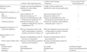
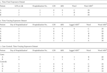
To conduct a cohort study with time-fixed exposures, we used a Cox model to estimate the risk factors for developing an infection during hospitalization (Table 1). The dataset was structured in a patient-hospitalization format such that each record represented a single hospitalization (Table 2A). The outcome was the number of days elapsed until the start of CDI, starting from day 3 of hospitalization. Lengths of stay of 1 or 2 days were excluded because the definition of hospital onset infection excludes cases developed <48 hours after admission.Reference McDonald, Coignard, Dubberke, Song, Horan and Kutty 23 Patients were considered censored if they experienced discharge or death without infection. A total of 4 individual-level risk factors and 1 ward-level risk factor were included in the model (Table 1). The baseline period was considered as days 1 to 2 of the hospitalization, with day 3 being the first day of the at-risk period.
Review of Differences Between the Modeling Strategies

NOTE. DOTs, days of therapy; TF, time-fixed; TV, time-varying.
*Same as modeling strategy 2.
Example Datasets for Time-Fixed Cohort, Time-Varying Cohort, and Time-Varying Case-Control Analyses.Footnote a

NOTE. ABX, antibiotic use; CDI, Clostridium difficile infection; LOS, length of stay.
a The 3 datasets represent 2 patients (A and B) that develop CDI during a given hospital stay, the first with onset on day 5 of their second hospitalization and the second with onset on day 4 of their first hospitalization. In the case-control dataset, note that patient A on day 4 of hospitalization acts as a control for case B. Also, 3 additional control patient days have been added to this dataset for illustration. These datasets also demonstrate the implementation of a lagged covariate (lagged ABX) and an ecological exposure measure (ward ABX).
b Mean ward-level antibiotic use (DOTs per 100 patient days).
c Days 1 and 2 of hospitalization are excluded from the analysis dataset because patients are not at risk of developing nosocomial CDI.
d Antibiotic exposure in the previous 7 days.
The statistical analysis used a Cox mixed-effects model with 2 random-effects levels. The first level corresponded to the ward in which a patient was located on day 3 of their hospitalization (n=16), and this accounted for spatial clustering of cases. The second level, nested within each of the wards, corresponded to the biannual period (December–May, June–November) on day 3 of the hospitalization. The biannual periods were made to align approximately with the high and low seasons of CDI; the high season peaks in early March in North America.Reference Brown, Daneman, Arora, Moineddin and Fisman 24 Because there were 16 wards and 9 biannual periods and 1 ward was closed in spring 2010, there were a total of 143 (16 × 9 – 1) biannual random intercepts. The nested biannual periods accounted for the temporal clustering of cases within wards.Reference Fielding and Goldstein 25
Approach 2: Cohort Study with Time-Varying Exposures
To conduct a cohort study with time-varying exposures, we used a time-varying Cox model to estimate the probability of developing an infection on a given day (Table 1). The data were structured in patient-day format with 1 record for each hospitalized patient day (Table 2B). Patient days when a patient was not hospitalized and also the days after a patient developed symptoms were excluded, as were the first 2 days of the hospital stay. The outcome variable was coded as 1 on the day when a given patient developed symptoms and zero otherwise. As with the time-fixed approach, 5 covariables (ie, 4 individual level, and 1 ward level) were included in the model. The statistical analysis utilized a Cox mixed-effects model with 2 random-intercept terms that were analogous to the time-fixed approach. The first corresponded to the ward in which a patient was located on a given day (to account for spatial clustering of cases within wards). The second corresponded to the biannual period and accounted for temporal clustering of outcomes within wards.Reference Fielding and Goldstein 25
Approach 3: Incidence-Density Sampling Case-Control Study
Starting from the patient-day dataset described above, 5 control patient days were selected for each case patient day, matching on at-risk day (Table 2C). To do so, we first categorized at-risk days into ~0.5% quantile bins and, for each bin with at least a single case patient day, we selected 5 control patient days. We then ran a conditional logistic regression model with covariates and random effects analogous to model 2. The strata corresponded to the at-risk days bins.
Parameter Estimates
Because conditional logistic regression is implemented within a Cox modeling framework, with strata corresponding to distinct failure times, each of the 3 models could be fit using the coxme function in R statistical software.Reference Therneau and Grambsch 11 Due to instability of the estimates from multilevel models,Reference Bolker, Brooks and Clark 20 estimates and confidence intervals for fixed- and random-effects parameters were based on the mean and the 2.5 and 97.5 percentiles from 500 bootstrap samplesReference Fox 26 (see Appendix 2).
Ethics Statement
Study approval was obtained from the Research Ethics Board of Sunnybrook Health Sciences Center. They waived the requirement for patient consent because there was no contact with patients and patient anonymity was assured.
RESULTS
Literature Scan
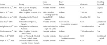
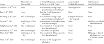
A total of 1,558 studies were identified that met our search criteria. After abstract and full-text review of the 50 most cited studies, 8 were retained (Tables 3A and 3B). As of November 2015, these 8 studies have been cited 2,500 times cumulatively since their publication and remain active, being cited 652 times since January 2013. Among these 8 studies, 2 failed to adjust for time at risk, 5 failed to assess the timing of exposures in a time window prior to outcome ascertainment, 6 failed to include ecological covariates, and 6 did not use methods to account for the clustering of outcomes in time and space. None of the studies accounted for spatial or temporal clustering of outcomes via random-effects or GEE models.
Characteristics of Studies Included in the Literature Scan

Results of the Literature Scan

NOTE. ID, incidence density; CDI, Clostridium difficile infection; LOS, length of stay; VRE, vancomycin-resistant enterococci; BSI, bloodstream infection; MRSA, methicillin-resistant Staphyloccocus aureus; hospit, hospitalization.
a Susceptible to time-dependent bias.
Cohort and Datasets
In total, there were 46,661 hospitalizations and 258 cases of CDI over the 46-month study period.Reference Brown, Valenta, Fisman, Simor and Daneman 22 The incidence rate of CDI was 6.0 per 10,000 patient days (258 of 428,588).
Parameter Estimates
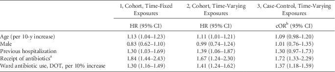
The cohort design with time-varying exposures and incidence density case-control design yielded largely similar results for all 5 covariables (Table 4). In both models, the strongest predictors were receipt of antibiotics in the previous 7 days (approach 2 hazard ratio [HR], 1.67; 95% confidence interval [CI], 1.24–2.30; approach 3 odds ratio [OR], 1.72; 95% CI, 1.33–2.29) and ward-level antibiotic exposures (approach 2 HR, 1.41; 95% CI, 1.24–1.62; approach 3 OR, 1.37; 95% CI, 1.18–1.59). The cohort design with time-fixed exposures measured associations for direct antibiotic receipt that were larger than the time-varying analyses (HR, 1.84; 95% CI, 1.44–2.43) and lower for ward-level antibiotic use (HR, 1.30; 95% CI, 1.16–1.49). Descriptions of the random-effects estimates from all 3 models are presented in Appendix 3.
Comparison of Coefficient Estimates from Hospitalization and Patient-Day Multivariate Analyses

NOTE. CI, confidence interval; DOT, days of therapy; HR, hazard ratio; cOR, conditional odds ratio.
a For time-fixed analysis, receipt of antibiotics was parameterized as receipt at any point during days 1, 2 or 3 of admission; for the patient-day level analysis, we measured any antibiotic receipt in the previous 7 days.
b The conditional odds ratios reported here approximate hazard ratios.
Sensitivity Analyses
We conducted 3 sensitivity analyses to investigate how estimates of antibiotic risk are impacted by time-dependent bias, under-adjustment for time at risk, and these 2 fallacies taken together. In the first sensitivity analysis, we used the dataset and model of approach 1, but we replaced baseline antibiotic measurement with antibiotic exposure at any point in time prior to, or on the day of, infection (rather than being limited to the baseline period). In this model, the risk of CDI associated with antibiotic receipt decreased (HR, 1.69; 95% CI, 1.20–2.37). In the second sensitivity analysis, we used the dataset and model of approach 1, but we specified a logistic mixed model with CDI during the at-risk period as the outcome rather than days to CDI. The estimated association for direct antibiotic use in this model was amplified (OR, 2.26; 95% CI, 1.71–2.97). For the third sensitivity analysis, we took the model from sensitivity analysis 2, but we replaced baseline antibiotic measurement with antibiotic exposure at any point in time prior to or on the day of infection. The estimated effect of direct antibiotic use in this model was strongly amplified (OR, 3.45; 95% CI, 2.47–4.81).
We conducted an additional sensitivity analysis to investigate how ignoring ward-level effects could impact estimates of direct antibiotic exposure risk. In this sensitivity analysis, we used the dataset and model of approach 2, but we removed both the ward antibiotic use and the ward and ward-period random intercepts. The estimated effect of direct antibiotic exposure in this sensitivity analysis (HR, 1.84; 95% CI, 1.41–2.40) was higher relative to the estimate that included ward-level factors (approach 2; HR, 1.67; 95% CI, 1.24–2.30).
DISCUSSION
The main findings of our literature review of HAI studies are the following: (1) underadjustment for time at risk and time-dependent confounding are common methodological issues in studies of HAIs, and (2) studies of HAIs tend not to model crucial environmental or group-level effects on infection risk. Our comparison of methods and sensitivity analyses demonstrated that (1) these issues can be addressed using standard statistical methods, and (2) failure to do so results in biased estimates of HAI risk factors.
Our literature review revealed that only 1 of 8 studies adjusted for both time-at-risk and was not subject to time-dependent confounding.Reference Pépin, Saheb and Coulombe 37 We found that, taken alone, the bias of risk estimates due to underadjustment for time at risk was positive, whereas the bias due to time-dependent confounding was negative. However, when both underadjustment for time at risk and time-dependent confounding were present, a strong positive bias in treatment effect was apparent. Indeed, the 1 study subject to this combination of issues demonstrated significant associations between almost all treatments and CDI risk, including the unusual result that receipt of intravenous vancomycin for >7 days increased the risk of CDI 18-fold in the unadjusted analysis and 1.9-fold in the adjusted analysis.Reference Dubberke, Reske, Yan, Olsen, McDonald and Fraser 27
Our literature scan revealed that only 2 of 8 studies considered ecological exposures as predictors of hospital infection risk. Further, of the 8 studies, only 2 accounted for correlated outcomes. Our review revealed a tendency for studies of nosocomial infection risk to ignore that the diseases under study are, at least partially, governed by the spread of infection. This tendency is surprising because infectious disease etiology is known to involve the movement of infectious particles in space. This result may indicate a tendency among biomedical researchers to falsely attribute group-level effects to individuals, also known as the atomistic fallacy.Reference Susser 15 Our sensitivity analyses demonstrated an overestimation of direct antibiotic exposure effects due to the failure to consider group-level effects of antibiotic exposures. More importantly, the failure to consider ecological effects in HAI risk-factor studies propagates the misunderstanding that HAI infections are caused primarily by intra-individual risk factors and that characteristics of hospital environments are not important subjects of study. Specific ecological measures that could be considered in many models of HAI risk prediction include average immunity (eg, vaccincation rates of patients or providers in a hospital), average infectiousness (eg, ward-level disease pressureReference Ajao, Harris and Roghmann 5 ), network structure (eg, hospital indegreeReference Simmering, Polgreen, Campbell, Cavanaugh and Polgreen 28 ), and physical structure (eg, hospital-bed size).
This study has several limitations. First, we restricted our review to a small number of the most frequently cited articles on HAI risk factors published since 2000, and as such, the articles selected were not a representative sample from the HAI risk-factor literature. Our selection likely overrepresented articles published in higher-impact English language journals, those published by more popular, high-status researchers, and those of above-average quality.Reference Siler, Lee and Bero 29 Second, for our comparison of methods, we chose to consider real-world data rather than base our analyses on simulated datasets. We preferred this approach to one involving simulations because our objective was to be as relevant as possible to investigators interested in HAI risk factors. However, we acknowledge that the interpretations we suggest do not necessarily reflect the true causes of differences between the models. Third, our approach to multilevel modeling attributed risks to wards in an imprecise manner. For the hospitalization-level models, the ward attribution was to the ward on the first day of the at-risk period and ignored wards that a patient visited later in the hospitalization. Ward effects in the patient-day analysis model were attributed to the ward where a patient was located on a given day but still ignored prior wards that a patient had visited. A more thorough approach would attribute risk to a mixture of prior wards using multiple-membership structures,Reference Fielding and Goldstein 25 though these approaches have not yet been implemented in statistical software packages. Alternatively, a dynamic individual-level transmission model could be implemented which represents our understanding of the actual transmission process, and parameters that govern disease latency and patient-to-patient transmission could be included.Reference Thomas, Redd, Khader, Leecaster, Greene and Samore 30 Even though such models may be the future gold standard for HAI risk-factor analysis, they have not been implemented in a fashion accessible to those without knowledge of Bayesian approaches and experience in statistical programming.
In the literature on HAI risk factors, the timing of exposures relative to outcomes is not correctly considered, and ecological exposures are often ignored. Our comparison of modeling approaches revealed biases due to underadjustment for the at-risk period, time-dependent confounding, and the failure to account for ecological exposures. Future studies of HAI processes should adequately account for the duration of the risk period, should guard against time-dependent bias, and should consider ecological risk factors whenever possible.
ACKNOWLEDGMENTS
Financial support: This research was supported by the VA Advanced Fellowship Program in Medical Informatics and by a doctoral research award from the Canadian Institute for Health Research.
Potential conflicts of interest: All authors declare no conflicts of interest relevant to this article.
APPENDIX 1: LITERATURE SCAN SEARCH STRATEGY
The search was conducted on Web of Science on November 4, 2014.
Search String
TOPIC: (Clostridium difficile OR MRSA OR VRE OR Pneumonia OR Hospital Acquired Infection) AND
TOPIC: (hospital OR inpatient OR length OR Stay) AND
TOPIC: (prediction OR cohort OR follow OR longitudinal OR prospective OR Inciden*) AND
NOT TOPIC: (cardiac OR diabetes OR dialysis OR sequencing) AND
NOT TOPIC: (cross-sectional OR surveillance OR mortality)
Refined by
Web of Science Categories: INFECTIOUS DISEASES OR MICROBIOLOGY AND
Document Types: ARTICLE AND
Timespan: 1970–2014 AND
Indexes: SCI-EXPANDED
APPENDIX 2. BOOTSTRAP METHODS
The measurement of random-effects variances in mixed-effects models is known to be unstable when the differences in incidence across clusters are small, when the number of clusters is small and when the number of cases per cluster is small.Reference Bell, Morgan, Kromrey and Ferron 38 , Reference Moineddin, Matheson and Glazier 39 Because estimates of fixed effects parameters depend on these unstable estimates of random-effects variances, bootstrappingReference Fox 26 is the most reliable and accessible method of obtaining confidence intervals from mixed-effects models.Reference Bolker, Brooks and Clark 20 Bootstrapping correctly propagates the instability of the random-effects variances into the confidence intervals of the fixed-effects parameters. Bootstrapping, in this study, involved picking many random subsets of the study observations, re-fitting the random effects model, and developing confidence intervals based on the lower and upper percentiles of the parameter estimates retrieved from each model.Reference Fox 26
APPENDIX 3. DESCRIPTION OF THE VARIANCE ESTIMATES
The hospitalization analyses included random intercepts corresponding to the hospital ward in which a patient was located on the first day of the at-risk period (day 3) and a further random effect for biannual period within that ward. The patient-day analysis included 2 analogous random effects corresponding to the location of a patient on a given day. In each of the 3 models, the standard deviation of the biannual-period effects was substantially larger than the ward-level effects (Table 1).
In a sensitivity analysis, we considered the impact of the covariance structure on the width of the confidence intervals for the fixed-effects. To do this, we compared the model from approach 1 to an analogous model without random effects and another analogous model with only ward-level random effects. For parameter estimates, the results were largely identical. However, the fixed-effects-only model underestimated the standard errors of the fixed-effects estimates by 9.1% (range, 5.0%–11.5%; Table). The model with ward-level random effects only under-estimated standard errors by 1.2% (range, −1.7%–2.8%).
Comparison of Model Random-Effects Estimates