Implications
Reproductive efficiency is a limiting factor in the production of Iberian pigs. This study showed that litter size in the Iberian pig can be increased through two non-exclusive strategies. The use of within-line selection is supported by the presence of sufficient additive genetic variation, and crossbreeding is supported by estimates of the crossbreeding effects derived from a full diallel experiment among three varieties (Entrepelado, Retinto and Torbiscal). In addition, the optimal hybrid sow can be produced by crossing a Retinto father and an Entrepelado mother.
Introduction
The Iberian pig breed is recognized as one of the porcine populations that has the highest meat quality (Serra et al., Reference Serra, Gil, Pérez-Enciso, Oliver, Vázquez, Gispert, Díaz, Moreno, Latorre and Noguera1998; Gandemer, Reference Gandemer2009), which is an important reason for its conservation because it has slower growth and lower feed efficiency (Barea et al., Reference Barea, Nieto, Vitari, Domeneghini and Aguilera2011) and prolificacy (Silió et al., Reference Silio, Rodriguez, Rodrigánez, Toro, Buxade and Daza2001) than do other commercial pig populations. Furthermore, a profound transformation that has involved the replacement of many traditional producers by intensive management farms has affected Iberian pig production. Normative that regulates the Iberian pig products forces that the sow is Iberian, whereas the boar could be either Iberian, Duroc (DU) or hybrid between these two breeds (Boletín Oficial del Estado, Reference Boletín Oficial del2014). In fact, a large proportion of Iberian pig farmers uses DU sires to obtain better growth rate and efficiency (Serrano et al., Reference Serrano, Valencia, Nieto, Lázaro and Mateos2008). Therefore, under intensive management, improvement in the reproductive efficiency of Iberian sows is essential for its economic viability.
The number of weaned piglets per sow in a year (or numerical productivity) is one of the most important factors in the profitability of pig farms, and litter size is its most important component (Quinton et al., Reference Quinton, Wilton, Robinson and Mathur2006; Dekkers et al., Reference Dekkers, Mather, Knol, Rothschild and Ruvisnky2011). Two non-exclusive strategies can lead to the genetic improvement of litter size: (1) within-line selection and (2) appropriate crossbreeding between lines to exploit heterosis.
Traditionally, genetic improvement in litter size in Iberian pig populations has been limited (Fernández et al., Reference Fernández, Rodrigáñez, Zuzúarregui, Rodríguez and Silió2008), and Iberian pig farmers have not used crossbred sows; rather, they have bred one of the varieties of the Iberian breed, exclusively (Martínez et al., Reference Martínez, Delgado, Rodero and Vega-Pla2000), which differed markedly from the practices used with other populations of commercial pigs in which selection efforts for prolificacy in maternal lines have been common and crossbreeding has been a standard procedure (Dekkers et al., Reference Dekkers, Mather, Knol, Rothschild and Ruvisnky2011). Several studies have identified genetic variability for prolificacy within (Rodríguez et al., Reference Rodríguez, Rodrigañez and Silio1994, Fernández et al., Reference Fernández, Rodrigáñez, Zuzúarregui, Rodríguez and Silió2008) and between (García-Casco et al., Reference García-Casco, Fernández, Rodríguez and Silió2012) varieties of Iberian pig. Thus, within-line selection and the implementation of a maternal crossbreeding scheme are plausible strategies for genetic improvement; however, to identify the most appropriate strategy, reliable estimates of the heritability of prolificacy in each population and estimates of the crossbreeding parameters as defined by the Dickerson’s model are required (Dickerson, Reference Dickerson1969).
The objective of this study was to estimate the additive genetic variation (or heritability) and the crossbreeding effects (direct, maternal and heterosis) for prolificacy using data from an experiment based on a full diallel design (Hayman, Reference Hayman1954) among three contemporary commercial varieties of Iberian pig [Entrepelado (E), Retinto (R) and Torbiscal (T)] under intensive management conditions. The overarching objective of the study was to identify suitable genetic improvement strategies within a pyramidal breeding program among the Iberian pig populations.
Materials and methods
Animals and experimental design
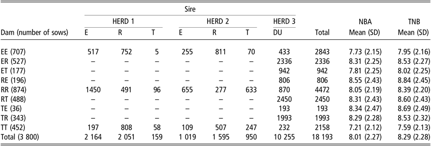
The data set comprised 18 193 records for total number born (TNB) and number born alive (NBA) from 3800 sows that had been obtained from a full diallelic experiment among three varieties of the Iberian pig breed (Retinto x Retinto (RR), Torbiscal x Torbiscal (TT) and Entrepelado x Entrepelado (EE)) and their reciprocal crosses (Retinto × Torbiscal (RT), Torbiscal × Retinto (TR), Retinto × Entrepelado (RE), Entrepelado × Retinto (ER), Torbiscal × Entrepelado (TE) and Entrepelado × Torbiscal (ET)). The three varieties are recognized in Spain’s official Iberian herd-book [Spanish Association of Iberian Purebred Pig Breeders (AECERIBER)]. A detailed description of their characteristics is provided by Ibáñez-Escriche et al. (Reference Ibañez-Escriche, Magallón, González, Tejeda and Noguera2016). Purebred sows were located in two nucleus herds in intensive management systems (Herds 1 and 2), and the service boars for these sows were kept at an artificial insemination center. A third herd (HERD 3) was a commercial production herd in which all sows, purebred or crossbred, were mated with boars from a DU population following the standard production system of Iberian pigs under intensive management. The distribution of the data between herds and breed of service sire and the average and SD of NBA and TNB for all crosses are presented in Table 1. In addition, the pedigree was extended back up to 3 generations, and it consisted of 4609 individuals. The number of founders in each per population was 47 Entrepelado (13 sires and 34 dams), 80 Retinto (18 sires and 62 dams) and 107 Torbiscal (38 sires and 69 dams).
Number of recorded parities by Iberian pig breed of sow, service sire and herd, and the mean and SD of the NBA and the TNB

E = Entrepelado; R = Retinto; T = Torbiscal; DU = Duroc; EE = Entrepelado × Entrepelado; ER = Entrepelado × Retinto; ET = Entrepelado × Torbiscal; RE = Retinto × Entrepelado; RR = Retinto × Retinto; RT = Retinto × Torbiscal; TE = Torbiscal × Entrepelado; TR = Torbiscal × Retinto; TT = Torbiscal × Torbiscal; NBA = number born alive; TNB = total number born.
Statistical analyses
TNB and NBA were analyzed with a multiple population repeatability model following García-Cortés and Toro (Reference García-Cortés and Toro2006), which can divide the additive genetic values into separate fractions depending on their genetic origin. The general model of the analysis was as follows:
 $${\bf{y}} = X{\bf{b}} + \mathop \sum \limits_{i = E,R,T}^3 Z_i {\bf a_i} + W{\bf p} + {\bf e}$$
where y is the vector of phenotypic records (TNB and NBA), b is the vector of systematic effects: order of parity (six levels: first, second, third, fourth, fifth and sixth and beyond), herd-year-season (85 levels), genetic line of service boar [four levels: E, R, T and DU] and the genetic line of the sow (LE, LR, LT for E, T and R, respectively), genetic line of the mother of the sow (ME, MR and MT for E, T and R, respectively) and heterosis (HER, HET and HRT between E and R, E and T and R and T, respectively) effects following Dickerson’s model (Dickerson, Reference Dickerson1969). Furthermore, ai is the vector of random additive genetic effects of pure and crossbred individuals of the ith line –E, R or T- (with 1934, 2748 and 1765 levels, respectively), p is the vector of the permanent effect of the sow (3800 levels) and e is the residuals vector; X and W are known incidence matrices that link fixed and permanent random effects with the vector y. Further, ZE, ZR and ZT are the matrices that links data with the random additive effects of each line with dimensions 18 193 × 1934, 18 193 × 2748 and 18 193 × 1765 levels, respectively. The model allows for a different additive genetic variance component for each genetic origin, whereas the permanent environmental (p) and the residual effects (e) were assumed homogeneous between lines.
The model assumed flat prior distributions for systematic effects (b) and multivariate Gaussian distributions for the additive (ai), permanent environmental (p) and residual effects (e). The permanent environmental effects and the residuals were assumed identically and independently distributed; therefore, their prior distribution was as follows:
 $${\bf{p}}\sim N\left( {0,I\sigma _p^2 } \right)\ {\bf{e}}\sim N\left( {0,I\sigma _e^2 } \right)$$
The assumed prior distribution for the additive effects was as follows:
 $${\bf a_E} \sim N\left( {0,A_E \sigma _{a_E }^2 } \right)\ \,{\bf a_R} \sim N\left( {0,A_R \sigma_{a_R }^2 } \right)\ \ {\bf a_T} \sim N\left( {0,A_T \sigma _{a_T }^2 } \right)$$
where AE, AR and AT are the partial relationship matrices generated by the founders of E, R and T, respectively. The calculation of those matrices was performed following the algorithm proposed by García-Cortés and Toro (Reference García-Cortés and Toro2006), and they are illustrated with a tiny example in the Appendix. Prior distributions for the variance components  $(\sigma _{(a_E )}^2 ,\sigma _{(a_R ,)}^2 \sigma _{(a_T )}^2 ,\sigma _p^2 \ and\ \sigma _e^2 )$ were uniform.
The above model leads to the following mixed model equations:
 $$\eqalign{{\left[ {\matrix{ {X'X} & {X'Z_E } & {X'Z_R } & {X'Z_T } & {X'W} \\ {Z_E 'X} & {Z_E 'Z_E + A_E^ - {{\sigma _e^2 } \over {\sigma _{a_E }^2 }}} & {Z_E 'Z_R } & {Z_E 'Z_T } & {Z_E 'W} \\ {Z_R 'X} & {Z_R 'Z_E } & {Z_R 'Z_R + A_R^ - {{\sigma _e^2 } \over {\sigma _{a_R }^2 }}} & {Z_R 'Z_T } & {Z_R 'W} \\ {Z_T 'X} & {Z_T 'Z_E } & {Z_T 'Z_R } & {Z_T 'Z_T + A_T^ - {{\sigma _e^2 } \over {\sigma _{a_T }^2 }}} & {Z_T 'W} \\ {W'X} & {W'Z_E } & {W'Z_R } & {W'Z_T } & {W'W + I{{\sigma _e^2 } \over {\sigma _p^2 }}} \\ } } \right]}\\ {{\left[ {\matrix{ \bf{\hat b} \\ \bf{\hat a_E } \\ \bf{\hat a_R } \\ \bf{\hat a_T } \\ \bf{\hat p} \\ } } \right] = \left[ {\matrix{ {X'y} \\ {Z_E 'y} \\ {Z_R 'y} \\ {Z_T 'y} \\ {W'y} \\ } } \right]}}$$
where  $A_E^ - ,A_R^ - and\;A_T^ - $ are the inverses of non-zero part of the population specific partial numerator relationship matrices (see the Appendix).
From that general full model (LMH), the following models were defined by fixing to zero the direct (MH), maternal (LH), heterosis (LM), direct and maternal (H), direct and heterosis (M) and maternal and heterosis effects (L). The analysis of each model was performed using a Gibbs sampling algorithm (Gelfand and Smith, Reference Gelfand and Smith1990) with a single long chain of 1 000 000 iterations, following a ‘burn in’ period of 250 000 iterations.
Model comparisons
The models were compared using the deviance information criteria (DIC) (Spiegelhalter et al., Reference Spiegelhalter, Best, Carlin and Van der Linde2002) and the logarithm of the conditional predictive ordinate (LogCPO) (Gelfand, Reference Gelfand, Gilks, Richardson and Spiegelhalter1996).
Deviance information criteria:
The DIC compares the global quality of two or more hierarchical models accounting for model complexity. For a particular model M, the DIC is defined as follows:
 $$DIC_M = 2\bar D_M - D\left( {{\bf{\bar \theta }}_{\bf{M}} } \right),$$
where  $\bar D_M $ is the posterior expectation of the deviance
 $D\big( {{\bf{\bar \theta }}_{\bf{M}} } \big)$ and
 $D\big( {{\bf{\bar \theta }}_{\bf{M}} } \big) = - 2log\big( {{p}\big({\bf{y}} {|{\bf{\bar \theta }}_{\bf{M}} } \big)} \big)$ is the deviance evaluated at the posterior mean estimate of the parameter vector
 $\big( {{\bf{\bar \theta }}_{\bf{M}} } \big)$. The computation of DIC comprises two terms,
 $\bar D_M $ is a measure of model fit and
 $\bar D_M - D\big( {{\bf{\bar \theta }}_{\bf{M}} } \big)$ is related to the effective number of parameters. Models that have the smallest DIC have the best global fit after accounting for model complexity.
Log marginal probability:
If we consider the data vector y = (yi, y–i), where y i is the i th datum and y–i is the vector of data with the ith datum deleted, the conditional predictive distribution has a probability density equal to the following:
 $$p\left( {y_i {\rm{|}}{\bf{y}}_{ - {\bf{i}}} } \right) = \mathop \smallint \int p\left( {y_i {\rm{|}}{\bf{y}}_{ - {\bf{i}}} ,{\bf{\theta }}} \right)p\left( {{\bf{\theta }}{\rm{|}}{\bf{y}}_{ - {\bf{i}}} } \right)d{\bf{\theta }},$$
where θ is the vector of unknown parameters and random effects in the model. Therefore, p(yi|y–i) can be interpreted as the probability of each datum given the remaining data and is the conditional predictive ordinate (CPO) for the i th datum. The pseudo log-marginal probability of the data is as follows:
 $$\sum\nolimits_i {ln \;p\left( {y_i {\rm{|}}{\bf{y}}_{ - {\bf{i}}} } \right)} .$$
A Monte Carlo approximation of the CPO (Gelfand, Reference Gelfand, Gilks, Richardson and Spiegelhalter1996) is  $\sum\nolimits_i {\ ln\ \hat p\left( {y_i {\rm{|}}{\bf{y}}_{ - {\bf{i}}} } \right)}$, where
 $\hat p\left( {y_i {\rm{|}}{\bf{y}}_{ - {\bf{i}}} } \right) = N\left[ {\mathop \sum \limits_{j = 1}^N {1 \over {p\left( {y_i {\rm{|}}\theta ^j } \right)}}} \right]^{ - 1}$, and N is the number of Markov chain Monte Carlo (MCMC) draws, and θj is the jth draw from the posterior distribution of the corresponding parameter. The higher the value of the LogCPO, the better the fit of the model to the data.
Results
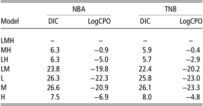
For both NBA and TNB, the model with best fit with DIC and LogCPO was the complete LMH model, followed by a group of models (LH, MH and H) whose differences from the best model ranged from 5.9 to 8.0 units for DIC and from 0.4 to 6.9 for LogCPO (Table 2). The LM, L and M models had a worse adjustment and their differences from the LMH model ranged from 22.4 to 26.6 for DIC and from 19.8 to 23.3 for LogCPO.
Differences with the best model for DIC and the LogCPO for NBA and TNB among three varieties of Iberian pig

LMH = full model with direct line; maternal and heterosis effects; MH = reduced model with maternal and heterosis effects; LH = reduced model with direct line and heterosis effects; LM = reduced model with direct line and maternal effects; L = reduced model with direct line effects; M = reduced model with maternal effects; H = reduced model with Heterosis effects; DIC=deviance information criteria; LogCPO = logarithm of the conditional predictive ordinate; NBA = number born alive; TNB = total number born.
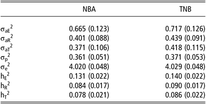
The posterior mean estimates (± posterior SDs) of the additive genetic variance ranged from 0.371 ± 0.106 (T) to 0.665 ± 0.123 (E) and from 0.418 ± 0.115 (T) to 0.717 ± 0.126 (E) for NBA and TNB, respectively, and the posterior mean estimates (± posterior SDs) of the permanent environmental and residual variances were 0.361 ± 0.051 and 4.020 ± 0.048 for NBA and 0.371 ± 0.053 and 4.029 ± 0.048 for TNB (Table 3). The posterior mean (± posterior SDs) estimates for the population-specific heritabilities were 0.078 ± 0.021 (T), 0.084 ± 0.017 (R) and 0.131 ± 0.022 (E) for NBA and 0.086 ± 0.022 (T), 0.090 ± 0.017 (R) and 0.140 ± 0.022 (E) for TNB. The results from the MH, LH, LM, L, M and H models were similar (Supplementary Tables S1 and S2 for NBA and TNB, respectively).
Posterior mean (and posterior SD) estimates [‘of’?] the additive  $(\sigma _{aE}^2 ,\,\sigma _{aR}^2 \,and\,\sigma _{aT}^2 )$, permanent environmental (σp2), and residual variance (σe2) components and population specific heritabilities (hE2, hR2, hT2) for NBA and TNB for each of three varieties of Iberian pig (Entrepelado (E), Retinto (R) and Torbiscal (T)) analyzed with full model with direct line, maternal and heterosis effect

NBA = number born alive; TNB = total number born.
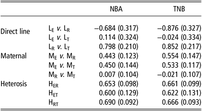
The posterior mean (± posterior SD) estimates of the differences between LE and LR, LE and LT and LR and LT were −0.684 ± 0.317, 0.114 ± 0.324 and 0.798 ± 0.210 for NBA and −0.876 ± 0.327, –0.024 ± 0.334 and 0.852 ± 0.217 piglets for TNB (Table 4). In addition, the posterior mean (± posterior SD) estimates of the differences of ME with MR and MT were 0.443 ± 0.123 and 0.450 ± 0.144 for NBA and 0.554 ± 0.117 and 0.533 ± 0.117 piglets for TNB. The differences between MR and MT were only 0.007 ± 0.104 and −0.021 ± 0.107. Those differences between the maternal effects were supported by the comparisons between reciprocals. The posterior mean (± posterior SD) estimates of the differences between ER and RE and between ET and TE were −0.443 ± 0.123 and −0.554 ± 0.125 and −0.450 ± 0.144 and −0.534 ± 0.147 for NBA and TNB, respectively. The differences between TR and RT were negligible (−0.007 ± 0.104 and 0.021 ± 0.107). Furthermore, the posterior mean (± posterior SD) estimates of the heterosis effects ranged from 0.600 ± 0.129 (HET) to 0.690 ± 0.092 (HRT) for NBA and from 0.622 ± 0.131 (HET) to 0.666 ± 0.093 (HRT) for TNB (Table 4). The results from the other models followed the same pattern (Supplementary Tables S3 and S4 for NBA and TNB, respectively).
Posterior mean (and posterior SD) estimates of the contrast between three varieties of Iberian pig for the direct line (LE, LR and LT) and maternal (ME, MR and MT) effects, and the heterosis (HER, HET and HRT) effects on NBA and TNB under the full model with direct line, maternal and heterosis effects

LE, LR and LT are the direct line effects for Entrepelado, Retinto and Torbiscal, respectively. ME, MR and MT are the maternal line effects for Entrepelado, Retinto and Torbiscal. HER, HET and HRT are the heterosis effects between Entrepelado and Retinto, Entrepelado and Torbiscal and Retinto and Torbiscal, respectively. NBA=number born alive; TNB=total number born.
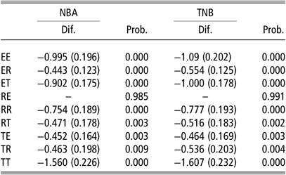
The posterior mean and SDs of differences between each cross with respect to the RE ranged from –0.443 (with ER) to –1.566 piglets (with TT) piglets for NBA and from –0.464 (with TE) to –1.607 (with TT) for TNB, and the posterior probability that RE is the best cross given the LMH model was 0.985 and 0.991 for NBA and TNB, respectively (Table 5).
Posterior mean (and SD) of the differences of the crosses (Dif.) with the Iberian pig population with the best performance (RE) and the posterior probability (Prob.) of being the best cross under the LMH model for NBA and TNB

EE = Entrepelado × Entrepelado; ER = Entrepelado × Retinto; ET = Entrepelado × Torbiscal; RE = Retinto × Entrepelado; RR = Retinto × Retinto; RT = Retinto × Torbiscal; TE = Torbiscal × Entrepelado; TR = Torbiscal × Retinto; TT = Torbiscal × Torbiscal; LMH = full model with direct line; maternal and heterosis effects. NBA = number born alive; TNB = total number born.
Discussion
The main advantage of the multiple population repeatability model proposed by García-Cortés and Toro (Reference García-Cortés and Toro2006) is that it provides specific estimates of the additive variance component (and heritability) for each population of origin and, therefore, it can detect differences in their genetic variation. The additive variance (and heritability) of the E variety was markedly higher than that of the other two populations (R and T) in all models. The estimates of the E population were higher than those obtained in previous studies of other Iberian pig populations (Pérez-Enciso and Gianola, Reference Pérez-Enciso and Gianola1992; García-Casco et al., Reference García-Casco, Fernández, Rodríguez and Silió2012), and the estimates for R and T were closer to such published estimates; however, estimates of heritability over 0.10 are common in white pig (Bidanel, Reference Bidanel, Rothschild and Ruvisnky2011; Putz et al., Reference Putz, Tiezzi, Maltecca, Gray and Knauer2015; Ogawa et al., Reference Ogawa, Konta, Kimata, Ishii, Uemoto and Satoh2018) and in Iberian populations (Fernández et al., Reference Fernández, Rodrigáñez, Zuzúarregui, Rodríguez and Silió2008). The results of our study should be confirmed based on a larger database; however, given the results of our study, it is plausible that the response to selection in the E population under an appropriate breeding scheme to improve litter size might be greater than it would be in the other lines. Thus, the E variety is a good candidate for inclusion in a pyramidal scheme for the improvement of litter size.
The results of the comparison of models indicated the importance of the direct line, maternal and heterosis effects based on both measures (LogCPO and DIC) because the LMH model had the best fit; however, the extent of this relevance was mixed. For example, the best model was followed closely by a group of models that share the effects of heterosis (LH, MH and H), which is reinforced by a posterior probability of a heterosis effect > 0 that was > 0.999 for all models and traits. Therefore, there was clear evidence of heterosis between each of the three potential crosses and small differences among them. A significant degree of heterosis was expected because it is common in crosses between pig populations (Haley et al. Reference Haley, Lee and Ritchie1995; Cassady et al., Reference Cassady, Young and Leymaster2002; García-Casco et al., Reference García-Casco, Fernández, Rodríguez and Silió2012). The results were surprising, however, because previous studies (Fabuel et al., Reference Fabuel, Barragán, Silió, Rodríguez and Toro2004) have suggested that the genetic distance between E and R is lower than the distance between either of them with T. Therefore, we expected a lower degree of heterosis between E and R than in crosses involving T.
The superiority of the LMH model over MH and the posterior distribution of the contrast between direct line effects in the LMH model confirmed the differences in the direct line effects on litter size. Numerous studies have reported differences in reproductive performance among swine populations (Bidanel, Reference Bidanel, Rothschild and Ruvisnky2011); thus, it is not surprising that this variability occurs among the Iberian varieties because the genetic diversity in Iberian pig populations is as high as it is among white pig populations (Martínez et al., Reference Martínez, Delgado, Rodero and Vega-Pla2000; Fabuel et al., Reference Fabuel, Barragán, Silió, Rodríguez and Toro2004). Over centuries, the Iberian pig has evolved adapting to harsh environmental conditions, and producers have subjected populations to ‘empirical’ selection in which adipogenic capacity and morphological criteria have played an important role. In addition, the small size of the herds and the degree of isolation between populations are other important factors. In general, the RR variety had the best line effects for prolificacy, and the E and T varieties had similar performances.
Furthermore, the best fit of LMH compared to the LH model and the posterior distribution of maternal effects provides evidence of its importance. The results indicated clearly the superiority (posterior probability > 0.99) of the maternal effect of the E variety over the R and T varieties, which was supported by the significant differences between reciprocals (RE v. ER and TE v. ET). In quantitative genetics, the importance of maternal effects is well recognized (Wilham, Reference Wilham1972; Wolf and Wade, Reference Wolf and Wade2009) and is typically found in growth traits in non-prolific species; however, few studies have reported on the maternal effects of sows on the litter size of their daughters. In addition, the estimates of the maternal effect on NBA and TNB were small (Southwood and Kennedy, Reference Southwood and Kennedy1990; Ferraz and Johnson, Reference Ferraz and Johnson1993; Irgang et al., Reference Irgang, Favero and Kennedy1994), which differs considerably from the results of our study, where the estimates of the differences between the maternal effects of the Dickerson’s model of the E variety compared to those of the R and T varieties were significant. Given the information available, the possible cause of that phenomena cannot be disentangled; however, recent studies on the genetic determinism of litter size in prolific species suggest a very complex panorama, which might permit speculation about a possible reason. The influence of maternal care on the reproductive performance of adult females has been investigated in rats (Cameron, Reference Cameron2011), which suggests that maternal behavior is transmitted to the next generation through epigenetic modifications such as methylation and histone acetylation, which is reflected in the variability in the expression of the estrogen receptor alpha. In addition, that phenomena is consistent with recent evidence of the effects of DNA methylation (Hwang et al., Reference Hwang, An, Kwon, Park, Kim, Kang, Yu, Kim, Park, Ha and Kim2017) and the presence of imprinted genes (Coster et al., Reference Coster, Madsen, Heuven, Dibbits, Groenen, van Arendonk and Bovenhuis2012) on litter size in pigs. Furthermore, apparently epistasis is a very important source of genetic variation in litter size in mice (Peripato et al., Reference Peripato, De Brito, Matioli, Pletscher, Vaugh and Cheverud2004) and swine (Noguera et al., Reference Noguera, Rodríguez, Varona, Tomás, Muñoz, Ramírez, Barragán, Arqué, Bidanel, Amills, Oviló and Sánchez2009). Another possibility is the effects of mitochondrial DNA, the variation of which has recently been associated with the maturation of oocytes in bovids (Srirattana et al., Reference Srirattana, McCosker, Schatz and John2017) and with the reproductive performance of daughters in pigs (Tsai et al. Reference Tsai, Rajasekar and John2016).
Despite the uncertainty about the biological basis of the results of this study, it has identified the clear advantage of crossbred over purebred individuals in litter size traits in the Iberian breed. Therefore, the implementation of a pyramidal scheme to provide crossbred sows to the producers is strongly recommended. Among the varieties investigated, the R population had the greatest direct line effect, and the E population had the greatest maternal effect and can provide a distinct advantage if it is used as the maternal line. The recommended cross for the practical implementation of a pyramidal scheme is R as the paternal and E as the maternal lines, which is supported by the posterior probability of being the best cross for NBA and TNB.
Acknowledgements
The authors gratefully acknowledge INGA FOOD SA and its veterinarians Emilio Magallón, M.J. García-Santana, Lourdes Muñoz, Pilar Diaz and Manuel Ramos for their cooperation with the experimental protocol and their technical support. The work was partially funded by the Center for Industrial Technological Development (CDTI) via grant IDI-20170304 and by grant CGL-2016-80155 from the Ministry of Economy, Industry and Competitiveness (MINECO), Spain. Preliminary results of this study were presented at the World Congress of Genetics Applied to Livestock Production (Noguera et al., Reference Noguera, Ibañez-Escriche, Magallón and Varona2018).
L. Varona 0000-0001-6256-5478
Declaration of interest
The authors declare that they have no competing interests.
Ethics statement
The research ethics committee of the Institute of Agrifood Research and Technology (IRTA) approved all of the management and experimental procedures involving live animals, which were performed in accordance with the Spanish Policy of Animal Protection RD1201/05, which complies with the European Union Directive 86/609 for the protection of animals used in experimentation.
Software and data repository resources
None of the data were deposited in an official repository. FORTRAN code is available from the corresponding author under reasonable request.
Supplementary material
To view supplementary material for this article, please visit https://doi.org/10.1017/S1751731119001125.
Appendix : Partial numerator relationship matrices and their generalized inverses
In order to illustrate the procedure of definition of the partial numerator relationship matrices required for the implementation of the procedure of García-Cortes and Toro (Reference García-Cortés and Toro2006), we have defined the following pedigree with purebred and crossbred individuals between three populations (A, B and C):

Given this genealogical information, the partial numerator relationship matrix for the A population is:
 $${A_A = \left[ {\matrix{ 1 & 0 & 0 & 0 & 0 & 0 & {0.5} & {0.5} & 0 & {0.5} & 0 & 0 \\ 0 & 1 & 0 & 0 & 0 & 0 & {0.5} & 0 & 0 & 0 & 0 & 0 \\ 0 & 0 & 0 & 0 & 0 & 0 & 0 & 0 & 0 & 0 & 0 & 0 \\ 0 & 0 & 0 & 0 & 0 & 0 & 0 & 0 & 0 & 0 & 0 & 0 \\ 0 & 0 & 0 & 0 & 0 & 0 & 0 & 0 & 0 & 0 & 0 & 0 \\ 0 & 0 & 0 & 0 & 0 & 0 & 0 & 0 & 0 & 0 & 0 & 0 \\ {0.5} & {0.5} & 0 & 0 & 0 & 0 & 1 & {0.25} & 0 & {0.25} & 0 & 0 \\ {0.5} & 0 & 0 & 0 & 0 & 0 & {0.25} & {0.5} & 0 & {0.25} & 0 & 0 \\ 0 & 0 & 0 & 0 & 0 & 0 & 0 & 0 & 0 & 0 & 0 & 0 \\ {0.5} & 0 & 0 & 0 & 0 & 0 & {0.25} & {0.25} & 0 & {0.5} & 0 & 0 \\ 0 & 0 & 0 & 0 & 0 & 0 & 0 & 0 & 0 & 0 & 0 & 0 \\ 0 & 0 & 0 & 0 & 0 & 0 & 0 & 0 & 0 & 0 & 0 & 0 \\ } } \right]}$$
The inverse of the non-zero part of this matrix  $(A_A^ - )$ can be calculated following the rules described by García-Cortés and Toro (Reference García-Cortés and Toro2006), given that
 $A_A^ - = \left( {I - P} \right)'D_X^ - \left( {I - P} \right)$. P is a matrix that relates progeny to parent and DX is recursively obtained by the algorithm described by Quaas (Reference Quaas1976). Therefore:
 $${A_A^ - = \left[ {\matrix{ {3.5} & {0.5} & - & - & - & - & { - 1} & { - 2} & 0 & { - 2} & - & - \\ {0.5} & {1.5} & - & - & - & - & { - 1} & 0 & 0 & 0 & - & - \\ - & - & - & - & - & - & - & - & - & - & - & - \\ - & - & - & - & - & - & - & - & - & - & - & - \\ - & - & - & - & - & - & - & - & - & - & - & - \\ - & - & - & - & - & - & - & - & - & - & - & - \\ { - 1} & { - 1} & - & - & - & - & 2 & 0 & 0 & 0 & - & - \\ { - 2} & 0 & - & - & - & - & 0 & 4 & 0 & 0 & - & - \\ - & - & - & - & - & - & - & - & - & - & - & - \\ { - 2} & 0 & - & - & - & - & 0 & 0 & 0 & 4 & - & - \\ - & - & - & - & - & - & - & { - - } & - & - & - & - \\ - & - & - & - & - & - & - & - & - & - & - & - \\ } } \right]}$$
Note that the inverse of the full AA matrix does not exist because of the existence of the non-zero part.
The partial numerator relationship matrix for the B population is
 $${A_B = \left[ {\matrix{ 0 & 0 & 0 & 0 & 0 & 0 & 0 & 0 & 0 & 0 & 0 & 0 \\ 0 & 0 & 0 & 0 & 0 & 0 & 0 & 0 & 0 & 0 & 0 & 0 \\ 0 & 0 & 1 & 0 & 0 & 0 & 0 & {0.5} & {0.5} & 0 & {0.5} & 0 \\ 0 & 0 & 0 & 1 & 0 & 0 & 0 & 0 & {0.5} & 0 & 0 & 0 \\ 0 & 0 & 0 & 0 & 0 & 0 & 0 & 0 & 0 & 0 & 0 & 0 \\ 0 & 0 & 0 & 0 & 0 & 0 & 0 & 0 & 0 & 0 & 0 & 0 \\ 0 & 0 & 0 & 0 & 0 & 0 & 0 & 0 & 0 & 0 & 0 & 0 \\ 0 & 0 & {0.5} & 0 & 0 & 0 & 0 & {0.5} & {0.25} & 0 & {0.25} & 0 \\ 0 & 0 & {0.5} & {0.5} & 0 & 0 & 0 & {0.25} & 1 & 0 & {0.25} & 0 \\ 0 & 0 & 0 & 0 & 0 & 0 & 0 & 0 & 0 & 0 & 0 & 0 \\ 0 & 0 & {0.5} & 0 & 0 & 0 & 0 & {0.25} & {0.25} & 0 & {0.5} & 0 \\ 0 & 0 & 0 & 0 & 0 & 0 & 0 & 0 & 0 & 0 & 0 & 0 \\ } } \right]}$$
With the following inverse:
 $${A_B^ - = \left[ {\matrix{ - & - & - & - & - & - & - & - & - & - & - & - \\ - & - & - & - & - & - & - & - & - & - & - & - \\ - & - & {3.5} & {0.5} & - & - & - & { - 2} & { - 1} & - & { - 2} & - \\ - & - & {0.5} & {1.5} & - & - & - & 0 & { - 1} & - & 0 & - \\ - & - & - & - & - & - & - & - & - & - & 0 & - \\ - & - & - & - & - & - & - & - & - & - & - & - \\ - & - & - & - & - & - & - & - & - & - & - & - \\ - & - & { - 2} & 0 & - & - & - & 4 & 0 & - & 0 & - \\ - & - & { - 1} & { - 1} & - & - & - & 0 & 2 & - & 0 & - \\ - & - & - & - & - & - & - & - & - & - & - & - \\ - & - & { - 2} & 0 & - & - & - & 0 & 0 & - & 4 & - \\ - & - & - & - & - & - & - & - & - & - & - & - \\ } } \right]}$$
Finally, the partial numerator relationship for the C population is
 $${A_C = \left[ {\matrix{ 0 & 0 & 0 & 0 & 0 & 0 & 0 & 0 & 0 & 0 & 0 & 0 \\ 0 & 0 & 0 & 0 & 0 & 0 & 0 & 0 & 0 & 0 & 0 & 0 \\ 0 & 0 & 0 & 0 & 0 & 0 & 0 & 0 & 0 & 0 & 0 & 0 \\ 0 & 0 & 0 & 0 & 0 & 0 & 0 & 0 & 0 & 0 & 0 & 0 \\ 0 & 0 & 0 & 0 & 1 & 0 & 0 & 0 & 0 & {0.5} & {0.5} & {0.5} \\ 0 & 0 & 0 & 0 & 0 & 1 & 0 & 0 & 0 & 0 & 0 & {0.5} \\ 0 & 0 & 0 & 0 & 0 & 0 & 0 & 0 & 0 & 0 & 0 & 0 \\ 0 & 0 & 0 & 0 & 0 & 0 & 0 & 0 & 0 & 0 & 0 & 0 \\ 0 & 0 & 0 & 0 & 0 & 0 & 0 & 0 & 0 & 0 & 0 & 0 \\ 0 & 0 & 0 & 0 & {0.5} & 0 & 0 & 0 & 0 & {0.5} & {0.25} & {0.25} \\ 0 & 0 & 0 & 0 & {0.5} & 0 & 0 & 0 & 0 & {0.25} & {0.5} & {0.25} \\ 0 & 0 & 0 & 0 & {0.5} & {0.5} & 0 & 0 & 0 & {0.25} & {0.25} & 1 \\ } } \right]}$$
And its inverse:
 $${A_C^ - = \left[ {\matrix{ - & - & - & - & - & - & - & - & - & - & - & - \\ - & - & - & - & - & - & - & - & - & - & - & - \\ - & - & - & - & - & - & - & - & - & - & - & - \\ - & - & - & - & - & - & - & - & - & - & - & - \\ - & - & - & - & {3.5} & {0.5} & - & - & - & { - 2} & { - 2} & { - 1} \\ - & - & - & - & {0.5} & {1.5} & - & - & - & 0 & 0 & { - 1} \\ - & - & - & - & - & - & - & - & - & - & - & - \\ - & - & - & - & - & - & - & - & - & - & - & - \\ - & - & - & - & - & - & - & - & - & - & - & - \\ { - - } & - & - & - & { - 2} & 0 & - & - & - & 4 & 0 & 0 \\ - & - & - & - & { - 2} & 0 & - & - & - & 0 & 4 & 0 \\ - & - & - & - & { - 1} & { - 1} & - & - & - & 0 & 0 & 2 \\ } } \right]}$$