1. Introduction: background and objectives
This study is concerned with the effects of stable buoyancy upon the evolution of a turbulent wake. These effects can be parameterized by the Froude number
 $Fr=U/NL$
, where
 $U$
and
 $L$
are relevant velocity and length scales and
 $N=[-g(\text{d}{\it\rho}/\text{d}z)_{\infty }/{\it\rho}_{\infty }]^{1/2}$
is the Brunt–Väisälä frequency (where
 $g$
is the gravitational acceleration,
 $(\text{d}{\it\rho}/\text{d}z)_{\infty }$
is the vertical gradient of the background density and
 ${\it\rho}_{\infty }$
is a characteristic/reference density). The Froude number is an inverse measure, being small when buoyancy is important and large when it is not. For the flow over a wake-generating body, an appropriate Froude number can be defined as
 $Fr_{\infty }=2V_{\infty }/ND$
, where
 $V_{\infty }$
and
 $D$
are the speed and effective cross-sectional diameter of the wake-generating body. A local time- (or downstream-distance)-dependent alternative is the deficit Froude number,
 $Fr_{d}=U_{d}/Nh$
, where
 $U_{d}$
is the maximum mean wake velocity deficit and
 $2h$
is the mean wake width. Since the velocity deficit decreases with distance from the body while the wake width increases, the wake Froude number strictly decreases with distance. This implies all wakes in stratified fluids will be affected by buoyancy at some point in their development.
Here, we consider the weakly stratified case with initially high Froude number (
 $Fr_{d}\gg 1$
), such that the wake is largely unaffected by buoyancy for some distance downstream of the body. Weakly stratified wakes evolve through three distinct regimes, which Spedding (Reference Spedding1997) referred to as the three-dimensional (3D), non-equilibrium and quasi-two-dimensional states. A review of the towed-wake experiments from which this picture derives is given by Diamessis, Spedding & Domaradzki (Reference Diamessis, Spedding and Domaradzki2011), while a model that recovers the three regimes, along with two others, is presented by Meunier, Diamessis & Spedding (Reference Meunier, Diamessis and Spedding2006). A summary of these three regimes as well as the open questions that we intend to study regarding the dynamics is given below.
During the 3D regime, the high-Froude-number wake is initially unaffected by buoyancy and thus produces fully three-dimensional turbulent motions for a period of time, while the wake-defect Froude number remains greater than order 1. The turbulence statistics are consistent with unstratified flows during this time and exhibit self-similar behaviour indistinguishable from that observed in unstratified wakes (Tennekes & Lumley Reference Tennekes and Lumley1972; Bevilaqua & Lykoudis Reference Bevilaqua and Lykoudis1978). This situation is in contrast to flows with
 $Fr_{d}$
of order one or smaller, which are immediately altered by stratification, so that the canonical self-similar state is never realized. In the extreme initial-
 $Fr_{d}\rightarrow 0$
case, buoyancy suppresses vertical motion to the extent that three-dimensional turbulence never appears (Chomaz et al.
Reference Chomaz, Bonneton, Butet and Hopfinger1993; Riley & Lelong Reference Riley and Lelong2000). For towed-sphere experiments, the critical value below which the 3D regime does not exist is
 $Fr_{\infty }\approx 4$
(cf. Dommermuth et al.
Reference Dommermuth, Rottman, Innis and Novikov2002).
When the initially three-dimensional turbulence in the high-
 $Fr_{\infty }$
wake begins to ‘feel’ the effects of buoyancy, the non-equilibrium (NEQ) (also known as ‘vertical-’ or ‘wake-collapse’) regime begins. (The term ‘non-equilibrium’ can be viewed as a synonym for ‘intermediate’ or ‘transitional’, and should not be interpreted literally: it does not imply, for example, that in the pre- or post-NEQ states the rates of production and dissipation of turbulence kinetic energy balance, since that type of equilibrium does not happen even in the purely unstratified self-similar benchmark.) When the wake enters the NEQ phase, it ceases to spread vertically; in fact, the height has been observed in some cases to slowly decrease with time during this period (Lin & Pao Reference Lin and Pao1979; Brucker & Sarkar Reference Brucker and Sarkar2010; Diamessis et al.
Reference Diamessis, Spedding and Domaradzki2011) (the latter for the self-propelled case) – although this may be at least in part a consequence of how the height is defined. As we will see below, a distinction should be made between the heights based on the mean defect (typically measured using a Gaussian curve fit) and on the extent of the wake turbulence (revealed, for example, by shadowgraph or dye visualizations).
As the wake stops spreading vertically, its lateral growth continues at roughly the same rate as observed during the 3D phase (Diamessis et al.
Reference Diamessis, Spedding and Domaradzki2011). (We reserve the term ‘lateral’ to indicate the direction aligned with the axis orthogonal to the streamwise–vertical plane.) Whether the rate of lateral spreading remains exactly or only approximately constant as the flow passes from the 3D to NEQ states is an open question. Brucker & Sarkar (Reference Brucker and Sarkar2010) cite different power-law exponents for the mean defect width during the different regimes, while Diamessis et al. (Reference Diamessis, Spedding and Domaradzki2011) propose
 $t^{1/3}$
behaviour for the entire wake history, from their relatively low-
 $Fr_{\infty }$
simulations. Conservation of mean streamwise momentum suggests that the product of the height, width and maximum velocity of the mean defect will tend to remain constant with time. (If the vertical–lateral shape of the mean defect were purely Gaussian, the height, width and
 $U_{d}$
product would remain exactly constant.) Therefore, since the temporal variation of the height and
 $U_{d}$
change upon entrance to the NEQ regime, it seems likely that of the width will also deviate from its
 $t^{1/3}$
3D evolution. We suspect that the discrepancy between Brucker & Sarkar’s and Diamessis et al.’s observations has its roots in the statistical uncertainty of their results, associated with their (and our) use of the temporal idealization to simulate the wake. To avoid this issue for the results presented here (and thereby address this discrepancy), we found it necessary to increase the size of the sample used to derive mean quantities, by increasing the streamwise size of the simulation domain (see below).
The NEQ period is also characterized by a large reduction in the rate of decay
 $|\text{d}U_{d}/\text{d}t|$
of the maximum mean defect velocity
 $U_{d}$
and the rate of decay
 $|\text{d}k/\text{d}t|$
of the turbulence kinetic energy (TKE)
 $k$
. Spedding (Reference Spedding1997) and others (e.g. Dommermuth et al.
Reference Dommermuth, Rottman, Innis and Novikov2002; Diamessis et al.
Reference Diamessis, Spedding and Domaradzki2011) have described these as ‘restratification’ effects, attributed to the transfer of gravitational potential energy (PE) to kinetic energy (KE) as the wake collapses, and heavy/cold fluid parcels fall and light/warm ones rise towards their original positions. Although this explanation is plausible and popular, it is not the only possibility, since the mean and turbulence kinetic energies can also be enhanced by modifications to their production and dissipation processes (cf. Brucker & Sarkar Reference Brucker and Sarkar2010).
From a statistical point of view, the role of buoyancy in altering
 $|\text{d}U_{d}/\text{d}t|$
is an indirect one. This can be seen by considering the transport equation for the mean kinetic energy (MKE)
 $\overline{u}_{i}\overline{u}_{i}/2$
(which we define with respect to
 $V_{\infty }$
, such that the streamwise component
 $\overline{u}\,\overline{u}/2$
is maximum at the wake centreline and goes to zero in the free stream), noting that only for the vertical component,
 $\overline{w}\,\overline{w}/2$
, does this equation contain a transfer term,
 $-g\overline{{\it\rho}}\,\overline{w}$
, involving exchange between MKE and mean potential energy (MPE). Testing the hypothesis that the NEQ regime behaviour of
 $U_{d}$
is driven by restratification effects requires examination of the terms in the mean streamwise momentum equation (see results below).
On the other hand, assessing the PE-to-KE explanation for the TKE enhancement observed in the NEQ regime is more straightforward, since the TKE transport equation contains a (buoyancy-transport) term,
 $-g\overline{{\it\rho}^{\prime }w^{\prime }}$
, representing exchange between TKE and the potential energy of the turbulence (TPE). In what follows, we present evidence supporting a picture of NEQ dynamics that is based on a combination of buoyancy effects, involving vertical collapse of the mean flow (
 $\partial \overline{w}/\partial z<0$
) near the wake centreline, and alterations to the turbulence structure, leading to profound changes of the magnitude and distribution of the Reynolds stresses, rather than direct transfer of potential to kinetic energy of the turbulence.
After the NEQ phase, the wake enters the quasi-two-dimensional (Q2D) state, characterized by the emergence of large-scale coherent structures. (Godeford & Cambon (Reference Godeford and Cambon1994) point out that ‘quasi-two-component’ is a more accurate description of flows like this, whose vertical motions have been strongly attenuated by stable buoyancy, since significant vertical variations of the other two components are not necessarily negligible. Nevertheless, to be consistent with previous studies, we shall continue to use ‘Q2D’ to refer to this aspect of the wake evolution.) The towed-sphere measurements of Chomaz et al. (Reference Chomaz, Bonneton, Butet and Hopfinger1993) revealed that flattened ‘pancake-like’ eddies eventually appear for both weak and strong stratification (cf. Spedding Reference Spedding2002). (Dommermuth et al. (Reference Dommermuth, Rottman, Innis and Novikov2002) refer to ‘compact and energetic vortex structures in the stratified late wake’.) The maximum mean velocity begins to decrease more quickly than it did during the NEQ regime, while the mean defect spreads laterally at a rate comparable to the 3D value. The vertical spreading also begins again, growing at a rate consistent with viscous diffusion (Meunier et al. Reference Meunier, Diamessis and Spedding2006; Brucker & Sarkar Reference Brucker and Sarkar2010; Diamessis et al. Reference Diamessis, Spedding and Domaradzki2011).
Aside from the three distinct evolutionary regimes, stratified wakes also appear to differ from their unstratified counterparts in that they much more readily achieve a universal state in the final period of decay. Unstratified wakes are known to display mean spreading rates and turbulence-to-mean ratios that vary with the shape of the wake-creating object (Bevilaqua & Lykoudis Reference Bevilaqua and Lykoudis1978) (although they eventually, at distances corresponding to thousands of body sizes downstream, relax to a universal value; see Redford, Castro & Coleman (Reference Redford, Castro and Coleman2012), referred to hereinafter as RCC). This non-universality has been traced to differences in the near-field turbulence structures shed from bodies of different shape. For the stratified counterpart, a significant body of data suggests that the structures of the early and late wake are unrelated, with pancake eddies ultimately resulting from a wide variety of initial states, some of which are non-turbulent or even non-wake-like (Bonnier, Bonneton & Eiff Reference Bonnier, Bonneton and Eiff1998; Gourlay et al.
Reference Gourlay, Arendt, Fritts and Werne2001; Diamessis et al.
Reference Diamessis, Spedding and Domaradzki2011; Pal, de Stadler & Sarkar Reference Pal, de Stadler and Sarkar2013). Furthermore, Spedding (Reference Spedding1997) showed that for sphere wakes, nominal universality is obtained for the mean defect history
 $U_{d}(t)/V_{\infty }$
when weighted by
 $Fr_{\infty }^{2/3}$
. This scaling was generalized to bodies of various shapes by Meunier & Spedding (Reference Meunier and Spedding2004) (see also Meunier et al.
Reference Meunier, Diamessis and Spedding2006) by accounting, via an effective diameter, for the net momentum extracted by the body.
While the basic dynamics of stratified wakes is relatively well understood, at least on a qualitative level, less is known about the detailed processes that drive the transitions between the 3D, NEQ and Q2D regimes. The objective of this work is to better understand these processes, using complete and accurate statistics from a direct numerical simulation of this flow. We aim to do the following.
-
(a) Determine with improved certainty the power-law estimates for the mean defect maximum velocity
 $U_{d}$
, height
$h_{z}$
and width
$h_{y}$
for the three flow regimes.
-
(b) Analyse the terms in the budgets of mean kinetic energy, mean streamwise momentum and turbulence kinetic energy, to quantify how buoyancy alters the
$U_{d}$
,
$h_{z}$
and
$h_{y}$
histories. Clarify the role of potential-to-kinetic energy transfer during the NEQ regime. -
(c) Demonstrate how the wake development is affected by the details of the initial condition used in the numerical simulation, comparing with earlier simulation results to explore the extent to which mean defect histories exhibit universality.


In § 2, the numerical approach, initialization strategy and direct numerical simulation (DNS) parameters are described. Section 3 documents the wake development in terms of histories of mean flow statistics and budgets of mean kinetic energy, mean momentum and turbulence kinetic energy. Closing comments and conclusions are summarized in § 4, followed by appendices A and B, which respectively address the relationship between the streamwise domain size and the uncertainty in the mean defect histories, and the spatial variation of the terms in the turbulence kinetic energy budget during the various stages of wake development.
The present paper is an abridged version of Redford, Lund & Coleman (Reference Redford, Lund and Coleman2014), to which the reader may refer for more detail regarding the numerical issues and for results that supplement those included here.
2. Problem formulation, numerical strategy and parameters
The issues raised above will be addressed using DNS of a wake at high
 $Fr_{\infty }$
and relatively high Reynolds number. To put this study in context, we mention the earlier simulations of stably stratified wakes generated by constant-velocity axisymmetric towed bodies performed, for high
 $Fr_{\infty }$
, by Gourlay et al. (Reference Gourlay, Arendt, Fritts and Werne2001) (via DNS), Diamessis et al. (Reference Diamessis, Spedding and Domaradzki2011) (large-eddy simulation – LES) and Brucker & Sarkar (Reference Brucker and Sarkar2010) (DNS), the latter as part of a study of differences between wakes downstream of towed and self-propelled bodies in high- and low-
 $Fr_{\infty }$
backgrounds (de Stadler & Sarkar’s (Reference de Stadler and Sarkar2012) DNS includes the effect of body acceleration for moderate stratification). Lower-
 $Fr_{\infty }$
cases have been simulated by Dommermuth et al. (Reference Dommermuth, Rottman, Innis and Novikov2002), using LES, and (for a range of Prandtl numbers) de Stadler, Sarkar & Brucker (Reference de Stadler, Sarkar and Brucker2010), using DNS. Provided that it can reach relevant Reynolds numbers (and produce accurate statistics), a numerical approach has many advantages, supplying detail not available from experiment. For example, Gourlay et al.’s (Reference Gourlay, Arendt, Fritts and Werne2001) DNS revealed the vortex-ring structure underlying the Q2D pancake eddies, while the LES of Diamessis et al. (Reference Diamessis, Spedding and Domaradzki2011) documented the presence of small-scale Kelvin–Helmholtz instabilities during the NEQ regime and its Reynolds-number dependence. Dommermuth et al.’s (Reference Dommermuth, Rottman, Innis and Novikov2002) low-
 $Fr_{\infty }$
LES quantified the relative importance of the terms in the mean- and turbulence-kinetic-energy budgets, during the NEQ and Q2D regimes, that ensue when the turbulence is immediately affected by buoyancy. Similar exercises were performed by Brucker & Sarkar (Reference Brucker and Sarkar2010) and de Stadler & Sarkar (Reference de Stadler and Sarkar2012) for their towed- and self-propelled-body flows.
Following Gourlay et al. (Reference Gourlay, Arendt, Fritts and Werne2001), Dommermuth et al. (Reference Dommermuth, Rottman, Innis and Novikov2002), Brucker & Sarkar (Reference Brucker and Sarkar2010), de Stadler et al. (Reference de Stadler, Sarkar and Brucker2010), Diamessis et al. (Reference Diamessis, Spedding and Domaradzki2011) and de Stadler & Sarkar (Reference de Stadler and Sarkar2012), we (as in RCC) invoke a Galilean transformation, and emulate the actual, spatially developing wake with a parallel-flow temporally developing idealization. The resulting streamwise homogeneity allows efficient DNS with a standard triply periodic fast Fourier transform (FFT)-based pseudospectral method (Gottlieb & Orszag Reference Gottlieb and Orszag1977). For the high-Froude-number flow studied here, vertical density variations are negligible compared with the background reference density
 ${\it\rho}_{\infty }$
, allowing stable stratification to be accounted for with the Boussinesq (divergence-free velocity) approximation. Molecular diffusion of the (temperature-dependent) density field is matched to that for the velocity field by assuming the Prandtl number
 ${\it\nu}/{\it\alpha}_{T}=1$
(cf. de Stadler et al.
Reference de Stadler, Sarkar and Brucker2010), where
 ${\it\nu}$
is the kinematic viscosity and
 ${\it\alpha}_{T}$
is the thermal diffusivity, both of which are assumed constant in space and time (and therefore independent of temperature). The pressure variable in the incompressible Navier–Stokes equations is eliminated using a velocity–vorticity formulation (Kim, Moin & Moser Reference Kim, Moin and Moser1987). A low-storage third-order temporal discretization (Spalart, Moser & Rogers Reference Spalart, Moser and Rogers1991) is applied to the nonlinear terms, while the viscous terms are treated analytically (Rogallo Reference Rogallo1981).
To account for the possibility of the wake generating significant internal/buoyancy waves, a ‘fringe’ region is adopted at the lateral and vertical edges of the periodic domain, to prevent the energy radiated in the waves from re-entering the domain, and spuriously affecting the wake dynamics (see also Brucker & Sarkar Reference Brucker and Sarkar2010). Details are provided in Redford et al. (Reference Redford, Lund and Coleman2014).
The coordinate
 $x=x_{1}$
denotes the streamwise/longitudinal direction, along the wake axis, with
 $u=u_{1}$
the corresponding streamwise velocity, defined such that positive values point ‘upstream’ and the maximum occurs at the centreline (figure 3). Because of the parallel-flow assumption, the uniform background/free stream velocity
 $V_{\infty }$
amounts to an arbitrary Galilean shift; we chose
 $V_{\infty }=0$
, which implies
 $u\rightarrow 0$
far from the wake centreline. The lateral (‘spanwise’) and vertical directions are respectively
 $y=x_{2}$
and
 $z=x_{3}$
(positive upwards), with velocities
 $v=u_{2}$
and
 $w=u_{3}$
, such that
 $x$
–
 $y$
planes are normal to the gravity vector
 $g_{i}=-g{\it\delta}_{i3}$
(which here is active from the very beginning of the simulation, at
 $t=0$
).
Based on our experience with DNS of unstratified turbulent wakes (RCC), the wake is initialized as a sequence of vortex rings, identical to case VR of RCC apart from the ring spacing (see their figure 1a), embedded in a stably stratified background with imposed constant/uniform mean density gradient
 ${\it\Gamma}=(\text{d}{\it\rho}/\text{d}z)_{\infty }<0$
. This strategy was found to be an efficient way to produce fully developed wake turbulence containing mature turbulent structures, which – while not necessarily corresponding to those generated by a specific wake-creating body in a real-world application – allows us to perform a numerical experiment that can be used to address the issues raised above (such as the effect of the details of the initial conditions on late-wake development).
In order to simulate the wake using periodic boundary conditions, the transported density variable (
 $=\overline{{\it\rho}}(z,t)+{\it\rho}^{\prime }(x,y,z,t)$
) is defined as the deviation from the background density field
 ${\it\rho}_{\infty }+z{\it\Gamma}$
(where the origin of the
 $z$
axis is, say, in the centre of the computational domain).
Regarding the initial velocity field, as in Shariff, Verzicco & Orlandi (Reference Shariff, Verzicco and Orlandi1994), each ring in the sequence is represented as a circular loop, of radius
 $r_{0}$
in
 $y$
–
 $z$
planes, of Gaussian azimuthal core vorticity
 ${\it\omega}_{{\it\theta}}$
, with
 ${\it\omega}_{{\it\theta}}=({\it\gamma}/{\rm\pi}{\it\delta}_{{\it\omega}}^{2})\exp [-(s/{\it\delta}_{{\it\omega}})^{2}]$
, where
 ${\it\gamma}$
is the ring’s circulation,
 $s^{2}=(x-x_{0})^{2}+(r-r_{0})^{2}$
,
 $r^{2}=(y-y_{0})^{2}+(z-z_{0})^{2}$
and
 $(x_{0},y_{0},z_{0})$
is the location of the centre of the ring in question. The length scale
 ${\it\delta}_{{\it\omega}}$
defines the thickness of the vortex core (chosen as
 ${\it\delta}_{{\it\omega}}=0.4r_{0}$
). The rings are spaced uniformly every
 $2{\rm\pi}r_{0}/3$
along the wake axis
 $(x,y_{0},z_{0})$
(RCC used
 $16{\rm\pi}r_{0}/27\approx 0.59{\rm\pi}r_{0}$
); the rings combine to induce an initial mean velocity defect of maximum velocity
 $U_{do}$
and width
 $h_{o}$
, the latter defined as the radial distance from the wake centreline to the location at which the mean streamwise velocity
 $\overline{u}$
is half of
 $U_{d}$
.
The turbulent velocity and density fields are the result of a nonlinear/bypass transition, which is triggered by a
 ${\rm\Delta}r=\pm 0.004r_{0}$
maximum radial displacement of the ring circumference, in the
 $y$
–
 $z$
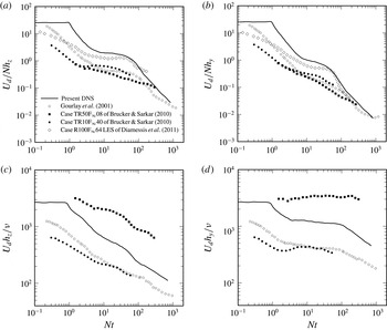
plane, for each of the azimuthal modes 5–32, with random azimuthal phases, using different random-number seeds for each ring. (The density fluctuations are initially zero, and develop in the gravitational field as the rings evolve.) As the individual vortex rings break down and disturb their neighbours, a varicose-type instability ensues (see figure 5a of RCC), leading to fully developed turbulence relatively quickly – much sooner than, for example, when very-small-amplitude disturbances are added to a mean defect profile, such that transition is via growth of the helical linear instability modes (as was done for case SD of RCC). The approach used by Gourlay et al. (Reference Gourlay, Arendt, Fritts and Werne2001) also avoids the need to simulate the natural linear instability transition process, by prescribing a Gaussian mean velocity and superimposing random finite-amplitude perturbations whose magnitudes are set by matching a desired energy spectrum, and then clipped/filtered in physical space with an axisymmetric/cylindrical window. Similar procedures were followed by Brucker & Sarkar (Reference Brucker and Sarkar2010) and Diamessis et al. (Reference Diamessis, Spedding and Domaradzki2011), although the former’s DNS involved an initial adjustment period during which the mean flow was held fixed as the fluctuations developed, and the latter’s LES required a precursor ‘relaxation’ simulation, during which the effective gravity was slowly increased. Despite being necessarily somewhat ‘synthetic’ in nature, those initialization schemes all produced statistics that very quickly exhibit expected behaviour (see figure 13). The primary difference between the present and earlier strategies is that here coherent structures are ‘hard-wired’ into the initial condition turbulence.
The initial Froude number specified here is quite large, to ensure that the wake turbulence is fully developed and physical when it is first affected by the stratification. The initial mean defect Froude number
 $Fr_{do}=U_{do}/Nh_{o}=23.7$
; this corresponds to
 $Fr_{\infty }=2V_{\infty }/ND$
of approximately
 $130$
, assuming the uniform flow speed
 $V_{\infty }\approx 5U_{do}$
and virtual-body diameter
 $D\approx 2h_{o}$
(see RCC). The initial mean defect Reynolds number
 $Re_{do}=U_{do}h_{o}/{\it\nu}=2625$
, such that the equivalent
 $Re_{\infty }=V_{\infty }D/{\it\nu}\approx 2.6\times 10^{4}$
. This is well above the critical value of
 $Re_{\infty }\approx 5\times 10^{3}$
, found by Spedding, Browand & Fincham (Reference Spedding, Browand and Fincham1996) to be required for the turbulent wake structures and decay rates to exhibit self-similarity – although it is not above the threshold (if one exists) beyond which all features (such as the duration of the various self-similar regimes) can be expected to be independent of Reynolds number (cf. Diamessis et al.
Reference Diamessis, Spedding and Domaradzki2011).
A significant computational challenge associated with this flow is the definition of an appropriate domain. Streamwise two-point correlations (shown in Redford et al.
Reference Redford, Lund and Coleman2014) indicate that the streamwise domain size
 ${\it\Lambda}_{x}$
used here is adequate throughout the simulation, and individual structures fit comfortably within the domain (since their streamwise integral scale is much smaller than
 ${\it\Lambda}_{x}$
), even at very late times. However, as mentioned above, the streamwise domain size also directly affects the quality of the mean statistics (and possibly the dynamics of the merging of the large-scale structures), since it defines the size of the ‘large-eddy sample’ (which will decrease as time passes) that enters the streamwise mean. Therefore, the choice was made to have a relatively large streamwise extent, with
 ${\it\Lambda}_{x}/h_{o}=96{\rm\pi}\approx 302$
(cf. Gourlay et al.’s (Reference Gourlay, Arendt, Fritts and Werne2001)
 ${\it\Lambda}_{x}/h_{o}=245$
, Brucker & Sarkar’s (Reference Brucker and Sarkar2010)
 ${\it\Lambda}_{x}/h_{o}\approx 105$
and Diamessis et al.’s (Reference Diamessis, Spedding and Domaradzki2011)
 ${\it\Lambda}_{x}/h_{o}\approx 54$
). The validity of this choice is demonstrated in appendix A (figure 15).
The possibility that the height and especially the width of the wake will outgrow the periodic domain is of even greater concern. To avoid this problem, without unduly wasting computational resources, the lateral and vertical domain sizes
 ${\it\Lambda}_{y}$
and
 ${\it\Lambda}_{z}$
are dynamically increased at appropriate times during the run, by prolongating the periodic solutions onto a domain of greater extent with the same grid spacing. The lateral domain is increased from
 ${\it\Lambda}_{y}/h_{o}=2{\rm\pi}$
at
 $Nt=0$
to
 $81{\rm\pi}$
at the end of the run,
 $Nt=841$
(where
 $t=0$
is the time at which the vortex-ring initial conditions are applied), while
 ${\it\Lambda}_{z}/h_{o}$
begins at
 $2{\rm\pi}$
and ends at
 $24{\rm\pi}$
. Details of this procedure are given in RCC; the domain variation history, and evidence to support its validity, are documented in Redford et al. (Reference Redford, Lund and Coleman2014).
The spatial resolution is also reduced during the simulations, as allowed by the monotonically decreasing Reynolds number. The number of streamwise
 $N_{x}$
, lateral
 $N_{y}$
and vertical
 $N_{z}$
equivalent grid points (quadrature/collocation points in physical space) ranges from a maximum of
 $N_{x}\times N_{y}\times N_{z}=4608\times 576\times 576\approx 1.5\times 10^{9}$
near the beginning of the run to a minimum of
 $384\times 288\times 144\approx 1.6\times 10^{6}$
near the end. (The
 $3/2$
rule is used to avoid aliasing errors when computing the nonlinear terms in physical space.) This ensures that the streamwise
 ${\rm\Delta}x$
, lateral
 ${\rm\Delta}y$
and vertical
 ${\rm\Delta}z$
grid spacings are small enough multiples of the minimum Kolmogorov scale
 ${\it\eta}_{min}$
throughout the simulation (between 1 and 4, except for a brief period at very early times when
 ${\rm\Delta}x$
reaches
 $7{\it\eta}_{min}$
) that we can safely assume that the results faithfully capture all the significant spatial scales of the turbulence. (The minimum Kolmogorov scale is defined as
 ${\it\eta}_{min}=({\it\nu}/{\it\epsilon}_{max})^{1/4}$
, where
 ${\it\epsilon}_{max}$
is the maximum of the streamwise mean rate of turbulence kinetic energy dissipation at each time.) The temporal scales are resolved by requiring the Courant–Friedrichs–Lewy (CFL) number defined by the low-storage third-order Runge–Kutta (RK3) scheme to not exceed
 $\sqrt{2.8}$
(Spalart et al.
Reference Spalart, Moser and Rogers1991) (this satisfies both stability and accuracy requirements; see appendix A).
A total of approximately 6000 CPU hours was expended on this case, running on between 32 and 128 processors of the UK EPSRC HECToR system.
3. Results
3.1. Averaging
Three types of averaging are used in this paper. The Reynolds decomposition is defined with respect to the mean (denoted by an overbar) formed by averaging over the homogeneous streamwise direction
 $x$
; this mean thus varies with lateral and vertical position, and time: e.g.
 $\overline{u}=\overline{u}(y,z,t)$
. (Note that, unlike for the unstratified wake simulated in RCC, averaging over the azimuthal direction is not appropriate.) A prime (
 $^{\prime }$
) indicates a deviation from this mean, such that the Reynolds stresses, density-fluctuation variance and turbulent buoyancy flux are written respectively as
 $-\overline{u_{i}^{\prime }u_{j}^{\prime }}$
,
 $\overline{{\it\rho}^{\prime }{\it\rho}^{\prime }}$
and
 $-\overline{{\it\rho}^{\prime }w^{\prime }}$
. As in Spedding (Reference Spedding1997), we also examine histories of bulk averages of Reynolds-averaged quantities, taken across the inhomogeneous directions (
 $y$
and
 $z$
) of the mean defect, over the region where
 $\overline{u}>0.05U_{d}$
; the shape and extent of this region are shown by the larger of the two closed solid-line contours in figures 6–9 and 17. (Spedding’s mean was over horizontal and vertical planes where
 $\overline{u}>0.2U_{d}$
.) These averages are indicated with angle brackets:
 $\langle k\rangle =\langle \overline{u_{i}^{\prime }u_{i}^{\prime }}\rangle /2=((\int _{0}^{{\it\Lambda}_{z}}\!\int _{0}^{{\it\Lambda}_{y}}{\it\psi}\overline{u_{i}^{\prime }u_{i}^{\prime }}\,\text{d}y\,\text{d}z)/2)/{\it\Psi}$
, where
 ${\it\psi}={\it\psi}(y,z)|_{\overline{u}/U_{d}>0.05}$
is unity if
 $\overline{u}(y,z)>0.05U_{d}$
and zero otherwise, and
 ${\it\Psi}=\int _{0}^{{\it\Lambda}_{z}}\!\int _{0}^{{\it\Lambda}_{y}}{\it\psi}\,\text{d}y\,\text{d}z$
. A third type of statistic (indicated by braces
 $\{~\}$
) is formed from cross-wake integration (not averaging) over the entire
 $y$
–
 $z$
domain, of Reynolds-averaged quantities; examples include the total/integrated turbulence kinetic energy (TKE)
 $\{k\}=(\int _{0}^{{\it\Lambda}_{z}}\!\int _{0}^{{\it\Lambda}_{z}}\overline{u_{i}^{\prime }u_{i}^{\prime }}\,\text{d}y\,\text{d}z)/2$
and its rate of production
 $\{\mathscr{P}_{tke}\}=-\!\int _{0}^{{\it\Lambda}_{z}}\!\int _{0}^{{\it\Lambda}_{z}}(\overline{u_{i}^{\prime }u_{j}^{\prime }}\partial \overline{u}_{i}/\partial x_{j})\,\text{d}y\,\text{d}z$
. A reasonable approximation of the cross-plane averages can be obtained from the cross-plane integrations by dividing the latter by the cross-sectional area of the mean defect, such that, e.g.,
 $\langle k\rangle \approx \{k\}/4{\rm\pi}h_{y}h_{z}$
.
3.2. Mean defect histories
3.2.1. Maximum mean and fluctuation velocities
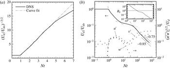
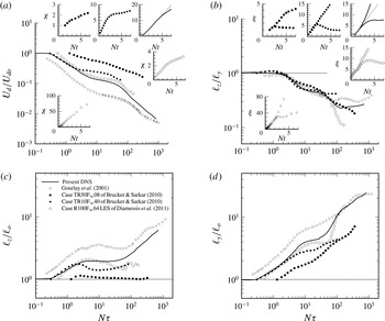
The history of the maximum mean velocity defect
 $U_{d}$
is shown in figure 1, in terms of the time
 $t$
after which the vortex-ring initial conditions were imposed. The
 $U_{d}(t)$
variation is smoother than that typically found from simulations, due to the reduced statistical oscillations associated with the larger than usual streamwise domain used here (the same can be said for the mean wake height and width histories in figure 2
a,b; see also appendix A). In contrast to the unstratified-wake DNS of RCC, for which the difference between the maximum and the centroid of the mean defect increases with time, and becomes significant at later stages, here there is essentially no difference between the two, for the time period considered. There is, however, a noticeable difference in the location in the
 $y$
–
 $z$
plane at which the two occur; as in RCC, we use the location of the centroid of the mean velocity distribution
 $\overline{u}(y,z)$
to define the current/local wake centreline coordinates
 $(y_{c},z_{c})$
.
Histories of the maximum mean velocity defect
 $U_{d}$
, buoyancy Reynolds number
 $Re_{b}$
and root-mean-square streamwise
 $u^{\prime }$
, lateral
 $v^{\prime }$
and vertical
 $w^{\prime }$
velocity fluctuations at the wake centreline. The curve fit in (a) is given by
 $(U_{d}/U_{do})^{-3/2}=3.1(Nt-0.645)$
, while in (b)
 $U_{d}/U_{do}=0.47(Nt-0.645)^{-2/3}$
shown for
 $Nt<10$
,
 $U_{d}/U_{do}=0.25(Nt+1.0)^{-1/4}$
for
 $3<Nt<100$
and
 $U_{d}/U_{do}=2.05(Nt-10)^{-0.85}$
for
 $Nt>30$
. The
 $U_{d}(t)$
interpolants in (b) intersect at
 $Nt\approx 6$
and
 $45$
. The buoyancy Reynolds number in the inset to (b) is defined as
 $Re_{b}=\{{\it\epsilon}_{tke}\}/4{\rm\pi}h_{y}h_{z}{\it\nu}N^{2}\approx \langle {\it\epsilon}_{tke}\rangle /{\it\nu}N^{2}$
.

Figure 1(b) also shows histories of the root-mean-squared streamwise
 $u^{\prime }$
, lateral
 $v^{\prime }$
and vertical
 $w^{\prime }$
velocity fluctuations at the wake centreline (symbols). These, along with the
 $U_{d}$
history, reveal that it is not until after
 $Nt\approx 1$
that the wake turbulence is fully developed. We therefore do not view the early phase, from
 $Nt=0$
until
 $Nt=Nt_{vo}\approx 1$
, as being representative of a turbulent wake. The exact virtual time origin
 $t_{vo}$
of the fully turbulent regime is defined by the unstratified 3D similarity diagnostic
 $U_{d}^{-3/2}$
shown in figure 1(a), from which we deduce
 $Nt_{vo}=0.645$
(chain-double-dotted line). In order to remove some of the uncertainty associated with comparing the present results during the 3D and NEQ regimes with those from experiments and other simulations, the histories that follow will be presented as functions of
 $N{\it\tau}=Nt-Nt_{vo}=Nt-0.645$
.
Figure 1(a) indicates that
 $U_{d}$
continues to exhibit pure 3D behaviour until
 $N{\it\tau}\approx 4.2$
, since this is when the similarity diagnostic first deviates from the linear variation. The early wake is well represented by the canonical
 $U_{d}\sim {\it\tau}^{-2/3}$
history despite not being fully self-similar during this time: although fully turbulent and essentially unstratified and axisymmetric (see figures 4 and 8a of Redford et al.
Reference Redford, Lund and Coleman2014), the wake’s non-dimensional Reynolds-shear-stress profile in cylindrical coordinates
 $-\overline{v_{x}^{\prime }v_{r}^{\prime }}/U_{d}^{2}$
(not shown) is not solely a function of the non-dimensional radius
 $r/h$
(i.e. with no time dependence). This is consistent with the evolution of the unstratified (vortex-ring-initialized) case VR wake described in RCC, for which (non-universal) self-similarity did not appear until after the time corresponding to
 $Nt\approx 11$
for the present simulation – and universal self-similarity not until
 $Nt>70$
. (For the present DNS, the relationship between
 $Nt$
and the non-dimensional time used in RCC is
 $t/t_{\ast }=30Nt$
.) In fact, in the range corresponding to
 $1<Nt<11$
, the
 $U_{d}$
history for case VR decays as
 $t^{-1}$
, because of the unique turbulence distribution induced by the case VR rings (which produce an eddy-viscosity profile that is temporally constant and radially uniform; see figures 8a and 9b of RCC; cf. Bonnier & Eiff (Reference Bonnier and Eiff2002), Nedic, Vassilicos & Ganapathisubramani (Reference Nedic, Vassilicos and Ganapathisubramani2013), de Stadler, Rapaka & Sarkar (Reference de Stadler, Rapaka and Sarkar2014)). Here, the ring initialization, which used somewhat larger streamwise spacing,
 $2.1h_{o}$
rather than case VR’s
 $1.85h_{o}$
, is such that
 $U_{d}\sim {\it\tau}^{-2/3}$
is a better representation than
 ${\it\tau}^{-1}$
for the 3D regime. These observations illustrate the profound impact the initial wake structure can have upon its early development.
As observed elsewhere (e.g. in Spedding’s (Reference Spedding1997) experiments and Gourlay et al.’s (Reference Gourlay, Arendt, Fritts and Werne2001) simulation), the magnitude of the rate of decay
 $|\text{d}U_{d}/\text{d}t|$
slows markedly for
 $Nt>5$
, as the flow enters the NEQ phase, such that
 $U_{d}\sim {\it\tau}^{-n}$
with
 $n\leqslant 1/4$
. In this region, the
 $U_{d}$
variation is well represented by the interpolant
 $0.25(Nt+1)^{-1/4}$
. (It should be mentioned that power laws with slightly different exponents could also reproduce the
 $U_{d}$
decay to good accuracy, given the flexibility afforded by the use of a finite virtual origin for time.) The time at which the 3D and NEQ power laws intersect,
 $N{\it\tau}\approx 5.5$
, can be viewed as an estimate of the boundary between the two regimes for the present flow. The generality of this finding will be discussed in § 3.7.
The
 $U_{d}$
-based NEQ period, beginning at
 $N{\it\tau}\approx 5.5$
, follows the NEQ power-law curve fit until approximately
 $N{\it\tau}=30$
. The Reynolds number of the present case is too low to allow an extended NEQ region. This is supported by the history of the buoyancy Reynolds number
 $Re_{b}$
(Ivey & Imberger Reference Ivey and Imberger1991; Hebert & de Bruyn Kops Reference Hebert and de Bruyn Kops2006) shown in figure 1(b) (inset), in that its value is less than one for
 $N{\it\tau}>17$
. Consequently, for the present DNS, the period during which significant turbulence is ‘regenerated’ by Kelvin–Helmholtz instabilities (Diamessis et al.
Reference Diamessis, Spedding and Domaradzki2011), if it exists at all, will be quite brief (see the instantaneous lateral vorticity contours at
 $N{\it\tau}=20$
in figure 5 of Redford et al. (Reference Redford, Lund and Coleman2014)). The Reynolds-number dependence of the duration of the NEQ regime will be considered in § 3.7. For now we note that the
 $U_{d}$
history seen here during the final stage of the NEQ phase is more consistent with the
 ${\it\tau}^{-1/2}$
behaviour of the ‘buoyancy-controlled’ subregion between NEQ and Q2D proposed by Meunier et al. (Reference Meunier, Diamessis and Spedding2006) than the
 $U_{d}$
plateau of the ‘NEQ
 $^{2}$
’ subregion identified by Brucker & Sarkar (Reference Brucker and Sarkar2010).
A
 ${\it\tau}^{-3/4}$
power law for
 $U_{d}$
could be assumed for the Q2D regime (cf. Spedding et al.
Reference Spedding, Browand and Fincham1996; Meunier et al.
Reference Meunier, Diamessis and Spedding2006), which would agree well with the present data for
 $Nt\geqslant 80$
if a virtual origin of
 $Nt=30$
were used. (Recall the earlier comment about the interplay between the power law’s exponent and the virtual origin.) However, a better fit is provided by
 ${\it\tau}^{-0.85}$
for
 $Nt\geqslant 60$
, with a smaller virtual origin (
 $Nt=10$
) (chain-double-dotted curve in figure 1
a). The
 $-0.85$
exponent is also more consistent with conservation of mean momentum, when coupled with the behaviour of the vertical and lateral defect dimensions (see below). The NEQ/Q2D boundary defined by the intersection of the corresponding power-law interpolants is
 $N{\it\tau}\approx 45$
. (A case could be made that another, perhaps more fundamental, definition of the NEQ/Q2D transition is provided by the
 $N{\it\tau}\approx 25$
corresponding to the beginning of the growth of the streamwise
 $u^{\prime }$
and lateral
 $v^{\prime }$
velocity fluctuations observed in figure 1
b; nevertheless, for convenience and to facilitate comparison with other studies, we have adopted the mean-defect-based definition for the present study.) The
 ${\it\tau}^{-0.85}$
interpolant closely corresponds to the
 $U_{d}$
variation from
 $N{\it\tau}\approx 50$
until the end of the simulation,
 $Nt\approx 840$
. It should be noted that the final time is not large enough for a purely viscous 3D regime to appear (which would yield
 $U_{d}\sim t^{-1}$
; see Meunier et al.
Reference Meunier, Diamessis and Spedding2006). In fact, the TKE remains a significant fraction of
 $U_{d}^{2}$
for all the times considered here (figure 10
a inset plot).
3.2.2. Mean height and width
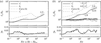
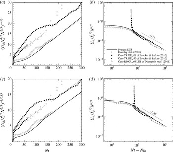
The height histories are shown in figure 2(a). Both the ‘half-radius’ height
 $h_{z}$
, i.e. half the distance between the locations at which the mean velocity in the vertical plane through the centreline,
 $\overline{u}(z,y_{c})$
, is 0.5 of
 $U_{d}$
(not a best fit to an assumed Gaussian profile), and an integral measure
 $r_{z}^{\ast }$
are shown; the latter is defined as
 $r_{z}^{\ast }=[(2\,\text{ln}\,2/U_{d})\!\int _{0}^{\infty }\overline{u}(r_{z},y_{c})r_{z}\,\text{d}r_{z}]^{1/2}$
, where
 $r_{z}^{2}=(z-z_{c})^{2}$
and
 $(y_{c},z_{c})$
are the coordinates of the local wake centreline. The integral height has been normalized such that it is equal to
 $h_{z}$
when
 $\overline{u}(z,y_{c})$
is Gaussian. Consequently, the greater the difference between
 $h_{z}$
(chain-dotted line) and
 $r_{z}^{\ast }$
(solid) in figure 2(a), the more non-Gaussian the vertical mean velocity profile (figure 3
a) will be. (Compare
 $h_{z}$
and
 $r_{z}^{\ast }$
values at
 $N{\it\tau}=20$
and the vertical mean profile
 $\overline{u}(z)$
at this time shown in figure 3
a, relative to the Gaussian idealization.)
During the 3D phase, when the wake is effectively unstratified, its height and width grow in proportion to
 ${\it\tau}^{1/3}$
, and its non-dimensional mean growth/spreading rate
 ${\it\beta}_{z}=(1/U_{d})\,\text{d}r_{z}^{\ast }/\text{d}t$
is approximately constant. Despite the wake not becoming fully self-similar, the spreading rate during the unstratified regime remains fixed near
 $0.03$
, which is roughly half that observed at much later times (corresponding to
 $Nt>70$
) for the self-similar growth of RCC’s unstratified case VR wake. (The streamwise velocity fluctuations at the centreline are also weaker here during the 3D regime than for case VR during its (first, non-universal) fully self-similar phase, with
 $(\overline{u^{\prime }u^{\prime }})_{c}^{1/2}/U_{d}\approx 0.2$
(open squares in figure 1
b) compared with approximately
 $0.3$
for case VR.) The 3D height/width interpolant deviates from the DNS sooner (near
 $N{\it\tau}=2$
) than the corresponding
 $U_{d}$
power-law interpolant does (
 $N{\it\tau}\approx 4.5$
). We also note that the mean defect does indeed ‘collapse’ early in the NEQ regime, in the sense that both
 $h_{z}$
and
 $r_{z}^{\ast }$
decrease with time from
 $N{\it\tau}\approx 8$
until approximately
 $N{\it\tau}=15$
, although the reduction in the integral height is much weaker than that exhibited by the
 $\overline{u}=0.5U_{d}$
measure
 $h_{z}$
. Regarding the Q2D period, figure 2(a) reveals, via its
 ${\it\tau}^{1/2}$
variation, the viscous nature of the vertical spreading of the mean wake for
 $N{\it\tau}>200$
or so; the non-dimensional vertical growth rate
 ${\it\beta}_{z}$
is therefore positive but much smaller than during the 3D regime, when the spreading is accomplished by the turbulence. The reasons for these phenomena – the differing times at which
 $U_{d}$
,
 $h_{z}$
and
 $h_{y}$
demonstrate NEQ behaviour, the mean height reduction with time during the NEQ regime and the controlling influence of viscous effects during the final phase of the wake evolution – will be presented in § 3.5.
Histories of mean wake length scales
 $\ell$
and growth rates
 ${\it\beta}$
in (a) the vertical and (b) the lateral direction. The curve fit for
 $\ell$
is given by
 $r_{z}^{\ast }/h_{o}=r_{y}^{\ast }/h_{o}=1.23(N{\it\tau})^{1/3}$
for
 $Nt<10$
, where
 $N{\it\tau}=Nt-Nt_{vo}$
and
 $Nt_{vo}=0.645$
(figure 13
b). At
 $Nt=0$
,
 $r_{z}^{\ast }=r_{y}^{\ast }=r_{o}^{\ast }=0.865h_{o}$
. The vertical and lateral growth rates are respectively
 ${\it\beta}_{z}=(1/U_{d})\,\text{d}r_{z}^{\ast }/\text{d}t$
and
 ${\it\beta}_{y}=(1/U_{d})\,\text{d}r_{y}^{\ast }/\text{d}t$
.

As mentioned in the introduction, due to the conservation of mean streamwise momentum, the product of the mean height, width and maximum velocity will remain fairly constant through the wake’s lifetime. (It would be exactly constant for a pure 2D (in
 $y$
and
 $z$
) Gaussian mean defect. The
 $U_{d}h_{y}h_{z}$
product for the present DNS remains most nearly constant during the 3D and especially late Q2D regimes, and varies most (and therefore exhibits the least Gaussian behaviour) during the NEQ state: compared with its value at
 $N{\it\tau}=0$
,
 $U_{d}h_{y}h_{z}$
is
 $0.84$
at
 $N{\it\tau}=2.5$
,
 $0.74$
at
 $N{\it\tau}=18$
,
 $0.71$
at
 $N{\it\tau}=82$
and
 $0.95$
at
 $N{\it\tau}=568$
.) The variations of the power-law exponents for
 $U_{d}$
and
 $h_{z}$
during the 3D, NEQ and Q2D regimes are thus expected to lead to variations of the mean width history, which would conflict with Diamessis et al.’s (Reference Diamessis, Spedding and Domaradzki2011) claim that
 $h_{y}\sim {\it\tau}^{1/3}$
for all three regimes. For example, the combination of monotonically decreasing
 $U_{d}$
and
 $\text{d}r_{z}^{\ast }/\text{d}t\rightarrow 0$
requires the mean width to grow faster than it does during the 3D phase as the wake approaches the NEQ regime, for
 $N{\it\tau}>1.5$
. Figure 2(b) illustrates the enhanced lateral growth, compared with the 3D power law (chain-double-dotted curve), in terms of both the mean half-width/radius
 $h_{y}$
(chained-dotted curve) and the integral width
 $r_{y}^{\ast }=[(2\ln 2/U_{d})\int _{0}^{\infty }\overline{u}(z_{c},r_{y})r_{y}\,\text{d}r_{y}]^{1/2}$
, with
 $r_{y}^{2}=(y-y_{c})^{2}$
(solid curve), for
 $1.5\leqslant N{\it\tau}\leqslant 4.5$
. Thereafter, the rate of spreading slows, falling from a maximum near
 $N{\it\tau}=5$
to a local near-zero minimum at
 $N{\it\tau}\approx 20$
(the closed diamonds in figure 2(b) show the history of the non-dimensional lateral spreading rate
 ${\it\beta}_{y}=(1/U_{d})\,\text{d}r_{y}^{\ast }/\text{d}t$
). Between
 $N{\it\tau}\approx 7$
and
 $30$
, when
 $U_{d}\sim {\it\tau}^{-0.25}$
and
 $\text{d}r_{z}^{\ast }/\text{d}t\approx 0$
, the
 $h_{y}$
history is reasonably well represented by
 ${\it\tau}^{1/8}$
variation (figure 2
b). The fact that these three exponents do not satisfy the Gaussian constant-momentum relation (i.e. that
 $-1/4+0+1/8\neq 0$
) is not a surprise, given that the
 $U_{d}h_{y}h_{z}$
product deviates most in the NEQ regime; the non-Gaussian nature of the defect during this time will be further illustrated below (see figures 3 and 7).
Beginning from
 $N{\it\tau}\approx 25$
, as the wake leaves the NEQ and enters the Q2D regime (and
 $U_{d}(t)$
begins to increase its rate of decay), the lateral growth increases rapidly until it reaches a value comparable to that observed during the unstratified 3D period, with
 $r_{y}^{\ast }\sim {\it\tau}^{0.35}$
. This is similar to the
 $h_{y}\sim {\it\tau}^{1/3}$
proposed by Diamessis et al. (Reference Diamessis, Spedding and Domaradzki2011), but differs from the
 ${\it\tau}^{1/4}$
included in Meunier et al.’s (Reference Meunier, Diamessis and Spedding2006) model, and the
 ${\it\tau}^{0.23}$
observed in Brucker & Sarkar’s (Reference Brucker and Sarkar2010) DNS, for the Q2D range. The difference between the
 $n=0.35$
and
 $0.25$
exponents is shown by the thin solid lines in figure 2(b), which supports our preference for the larger value – which in turn explains (in light of the viscous
 $n=1/2$
growth of
 $h_{z}$
, the near-Gaussian behaviour of the mean defect at late times and the conservation of momentum) our use of
 $n=-0.85$
to fit the
 $U_{d}(t)$
history (figure 1
b). (Meunier et al.’s (Reference Meunier, Diamessis and Spedding2006) exponent combination of
 $(-3/4,1/2,1/4)$
for
 $(U_{d},h_{z},h_{y})$
also satisfies the Gaussian/constant-momentum constraint.) Despite the profound qualitative differences in the turbulence structure in the 3D and Q2D regimes, the rates at which the mean defect spread laterally are approximately the same.
3.2.3. Comparison with height and width of turbulence
Figure 2(a) also shows the differences in the evolution of the height of the mean defect and vertical extent of the wake turbulence, which become apparent when one compares histories of
 $h_{z}$
(chain-dotted curve) or
 $r_{z}^{\ast }$
(solid) with that of
 $r_{z}^{\dagger }$
(dashed), a TKE-based integral length, defined as
 $r_{z}^{\dagger }=(\{k(z-z_{c})^{2}\}/\{k\})^{1/2}$
, where
 $k=\overline{u_{i}^{\prime }u_{i}^{\prime }}/2$
. As found by Gourlay et al. (Reference Gourlay, Arendt, Fritts and Werne2001), the turbulent region continues to spread vertically during the NEQ regime, when
 $\text{d}r_{z}^{\ast }/\text{d}t\approx 0$
, before an even more dramatic collapse occurs, with
 $\text{d}r_{z}^{\dagger }/\text{d}t<0$
(much larger than the negative
 $\text{d}h_{z}/\text{d}t$
and
 $\text{d}r_{z}^{\ast }/\text{d}t$
seen earlier) between
 $N{\it\tau}\approx 20$
and
 $100$
. This behaviour was also observed for the self-propelled case by Lin & Pao (Reference Lin and Pao1979) in their flow visualization experiments, and in Brucker & Sarkar’s (Reference Brucker and Sarkar2010) DNS of self-propelled and towed wakes.
After the wake enters the Q2D regime,
 $r_{z}^{\dagger }$
begins to grow again, as do
 $h_{z}$
and
 $r_{z}^{\ast }$
. All three heights then converge, as the vertical spreading becomes a purely viscous phenomenon, such that
 $h_{z}\approx r_{z}^{\ast }\approx r_{z}^{\dagger }$
(cf. Gourlay et al.
Reference Gourlay, Arendt, Fritts and Werne2001), and each grows as
 ${\it\tau}^{1/2}$
(Meunier et al.
Reference Meunier, Diamessis and Spedding2006). This can be seen in figure 8 of Redford et al. (Reference Redford, Lund and Coleman2014), which includes contours of the mean defect and TKE at times representing the three regimes; the trend is for the height of the turbulent region to occupy a smaller and smaller fraction of the mean defect as time passes.
The width of the turbulence, like that of the mean defect, grows continuously throughout the lifetime of the wake. This is shown by the history of the TKE-based integral width
 $r_{y}^{\dagger }=(\{k(y-y_{c})^{2}\}/\{k\})^{1/2}$
in figure 2(b) (dashed line). In contrast to the height of the turbulent region, its width remains significantly larger than the width of the mean defect, with
 $r_{y}^{\dagger }/h_{y}>1$
for each of the 3D, NEQ and Q2D periods (cf. Gourlay et al.
Reference Gourlay, Arendt, Fritts and Werne2001). (We cannot say whether or not the waviness in
 $r_{y}^{\dagger }(t)$
for
 $N{\it\tau}>20$
is physical; in view of the early-
 $h_{y}$
histories shown in appendix A, we suspect that it is not.) The closed and open circles in figure 2(b) respectively correspond to the ratios
 $L_{{\it\sigma}}^{\dagger }/r_{y}^{\ast }$
and
 $L_{{\it\sigma}}^{\ddagger }/r_{y}^{\ast }$
, where
 $L_{{\it\sigma}}^{\dagger }$
and
 $L_{{\it\sigma}}^{\ddagger }$
are, respectively, the distances from the wake centreline to the maximum values of the lateral Reynolds shear stress
 $-\overline{u^{\prime }v^{\prime }}$
and the horizontal-plane velocity fluctuations
 $(\overline{u^{\prime }u^{\prime }}+\overline{v^{\prime }v^{\prime }})^{1/2}$
. Integral versions of these scales are used, based on the profiles presented in Meunier & Spedding (Reference Meunier and Spedding2004), with
 $L_{{\it\sigma}}^{\dagger }\equiv \int _{-\infty }^{\infty }|\overline{u^{\prime }v^{\prime }}|\,\text{d}y/u_{0}^{\dagger 2}$
and
 $L_{{\it\sigma}}^{\ddagger }\equiv \int _{-\infty }^{\infty }(\overline{u^{\prime }u^{\prime }}+\overline{v^{\prime }v^{\prime }})^{1/2}\,\text{d}y/(2{\rm\pi})^{1/2}u_{0}^{\ddagger }$
, where
 $u_{0}^{\dagger 2}=\exp (0.5)(\overline{u^{\prime }v^{\prime }})_{max}$
,
 $u_{0}^{\ddagger }=0.5\exp (0.5)(\overline{u^{\prime }u^{\prime }}+\overline{v^{\prime }v^{\prime }})_{max}^{1/2}$
, and
 $(\overline{u^{\prime }v^{\prime }})_{max}$
and
 $(\overline{u^{\prime }u^{\prime }}+\overline{v^{\prime }v^{\prime }})_{max}^{1/2}$
are the maxima over
 $y$
of
 $|\overline{u^{\prime }v^{\prime }}|$
and
 $(\overline{u^{\prime }u^{\prime }}+\overline{v^{\prime }v^{\prime }})^{1/2}$
respectively.
In contrast to
 $r_{y}^{\dagger }/r_{y}^{\ast }$
, which is always significantly greater than one, the shear stress width ratio
 $L_{{\it\sigma}}^{\dagger }/r_{y}^{\ast }$
remains close to unity for the entire run, slightly less before
 $N{\it\tau}\approx 10$
, slightly more thereafter, while for the horizontal TKE measure
 $0.7<L_{{\it\sigma}}^{\ddagger }/r_{y}^{\ast }\leqslant 1$
throughout. The
 $L_{{\it\sigma}}^{\dagger }\approx r_{y}^{\ast }$
and
 $L_{{\it\sigma}}^{\ddagger }\approx r_{y}^{\ast }$
behaviour, which is similar to that exhibited by the experimental data for various bluff bodies given in Meunier & Spedding (Reference Meunier and Spedding2004), implies a type of self-similarity for the lateral profiles, especially for
 $-\overline{u^{\prime }v^{\prime }}$
, that survives as the importance of stratification and viscous effects grows, and the flow moves through the 3D, NEQ and Q2D regimes. The relationship between the spatial distributions of the turbulence and the mean defect is further illustrated in figures 6–9 of § 3.5.
3.3. Mean velocity profiles
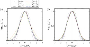
Figure 3 contains vertical and lateral profiles of the streamwise mean velocity
 $\overline{u}$
, normalized by the local maximum
 $U_{d}$
and height
 $h_{z}$
or width
 $h_{y}$
of the defect. The better collapse and smoother profiles seen here, compared with those from Gourlay et al.’s (Reference Gourlay, Arendt, Fritts and Werne2001) DNS and Diamessis et al.’s (Reference Diamessis, Spedding and Domaradzki2011) LES, are thought to be an indication of the better averaging sample afforded by the present larger streamwise domain. Included in these plots are results from times corresponding to the 3D, NEQ and Q2D regimes. (The dotted profile is the mean induced by the vortex-ring initialization.) Given the qualitative differences in the 3D, NEQ and Q2D turbulence structures (Redford et al.
Reference Redford, Lund and Coleman2014), the collapse at these times is striking, as is the agreement with the Gaussian idealization (open symbols), particularly near the centreline. At the earlier times, the non-Gaussian behaviour away from the centreline may be an artefact of the vortex-ring initialization, and/or due to attenuation of the turbulent transport, associated with corrugations of the interface between the vortical and irrotational regions (Townsend Reference Townsend1976) (see figure 4 of Redford et al.
Reference Redford, Lund and Coleman2014).
Profile of the mean streamwise velocity in (a) the vertical and (b) the lateral plane through the wake centreline. The Gaussian idealization is
 $\overline{u}/U_{d}=\exp (-\!\ln (2)s^{2})$
, where
 $s$
is either
 $(y-y_{c})/h_{y}$
or
 $(z-z_{c})/h_{z}$
. The coordinates
 $(y_{0},z_{0})$
and
 $(y_{c},z_{c})$
respectively define the initial and current location of the wake centreline, given by the centroid of the mean velocity defect.

For the lateral profiles, which tend to be more consistently Gaussian than the vertical ones, the near-centreline agreement is similar to that found by Spedding et al. (Reference Spedding, Browand and Fincham1996). (The unphysical lateral asymmetry at
 $N{\it\tau}=137$
is evidence of the finite eddy sample at this time. Curiously, the
 $\overline{u}(z_{c},y)$
profile at
 $N{\it\tau}=586$
, which is the result of averaging over an even smaller number of eddy structures than are present at
 $N{\it\tau}=137$
, is nearly exactly symmetric; see the long-dashed curve in figure 3
b.) The vertical profiles, on the other hand, can at times exhibit significant non-Gaussian features across the entire wake. One might suspect that the ‘extra peakiness’ near the centreline during the early stages of the Q2D regime (
 $N{\it\tau}=82$
and
 $137$
) is due to coarsening of the vertical resolution across the mean defect (see table 1 of Redford et al.
Reference Redford, Lund and Coleman2014). However, this possibility was ruled out by repeating this portion of the simulation with reduced (half) vertical grid spacing
 ${\rm\Delta}z$
, resulting in
 $\overline{u}(z,y_{c})$
variations that are nearly indistinguishable from those shown in figure 3(a).
3.4. Integrated mean kinetic energy history and budget
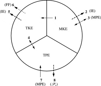
The mechanisms responsible for the mean defect evolution revealed in figures 1–3 can be further understood by examining the history and budget of the mean kinetic energy, which are presented in this section. As an aid to the discussion to follow, a diagram summarizing the transfers associated with the mean kinetic and potential energies (MKE and MPE), and the turbulence kinetic and potential energies (TKE and TPE) is given in figure 4 (see figure caption and (3.1) and (3.6) for definitions). In this section, we are concerned with terms 1, 2 and 3 respectively: the MKE-to-TKE transfer (i.e. TKE production), the MKE dissipation (loss to internal energy IE) and MKE-to-MPE exchange.
Transfer terms in the budgets of the mean kinetic energy
 $\text{MKE}=\overline{u}_{i}\overline{u}_{i}/2$
(3.1), turbulence kinetic energy
 $\text{TKE}=\overline{u_{i}^{\prime }u_{i}^{\prime }}/2$
(3.6), and turbulence potential energy
 $\text{TPE}=(g\overline{{\it\rho}^{\prime }{\it\rho}^{\prime }}/2)/{\it\rho}_{\infty }|{\it\Gamma}|$
:
1, TKE production
 $\mathscr{P}_{tke}$
(from MKE); 2, MKE dissipation
 $D_{iijj}$
(transfer to internal/thermal energy IE); 3, Mean buoyancy transfer
 $\mathscr{B}_{mke}=-g\overline{{\it\rho}}\,\overline{w}/{\it\rho}_{\infty }$
(exchange with mean potential energy
 $\text{MPE}=(g\overline{{\it\rho}}\,\overline{{\it\rho}}/2)/{\it\rho}_{\infty }|{\it\Gamma}|$
);
4, Turbulent buoyancy transfer
 $\mathscr{B}_{tke}$
(exchange with TPE); 5, TKE dissipation
 ${\it\epsilon}_{tke}$
(transfer to IE); 6, internal-wave radiation
 $\mathscr{W}_{tke}$
(lost to far field FF); 7, TPE production
 $-g(\overline{{\it\rho}^{\prime }u_{i}^{\prime }}/{\it\rho}_{\infty }|{\it\Gamma}|)(\partial \overline{{\it\rho}}/\partial x_{i})$
(from MPE); 8, TPE dissipation
 $({\it\alpha}_{T}g/{\it\rho}_{\infty }|{\it\Gamma}|)\overline{(\partial {\it\rho}^{\prime }/\partial x_{i})(\partial {\it\rho}^{\prime }/\partial x_{i})}$
(entropy production
 ${\mathcal{P}}_{s}$
due to heat conduction). See (3.1) and (3.6) for definitions relating to MKE and TKE budgets, and, e.g., Kundu (Reference Kundu1990) regarding MPE and TPE budgets. Single solid-line arrows indicate ‘production’ terms, with direction defined such that term acts as source. Dashed-line arrows denote irreversible sinks.

(a) Components of the integrated mean kinetic energy
 $\{K_{{\it\alpha}{\it\alpha}}\}=\{\overline{u}_{{\it\alpha}}\overline{u}_{{\it\alpha}}/2\}$
(no sum on
 ${\it\alpha}$
). Values are normalized by the MKE at
 $Nt=0$
,
 $\{K_{ii}\}_{o}=\{K_{11}\}_{o}+\{K_{22}\}_{o}+\{K_{33}\}_{o}$
. (b) Dominant terms in the budget of the MKE components, in units of
 $U_{r}^{3}L_{r}$
, where
 $U_{r}=2.09U_{do}$
and
 $L_{r}=h_{o}$
. (These arbitrary scales are implicitly defined by the non-dimensionalization used to prescribe the radius, spacing and circulation of the vortex rings in the initial condition field.) One should note the signs of
 $\{P_{2222}\}$
and
 $\{\mathscr{B}_{mke}\}=\{B_{33}\}$
(open symbols), which (unlike all the other terms) both act as sources in their respective
 $+\text{d}\{K_{{\it\alpha}{\it\alpha}}\}/\text{d}t$
balances.

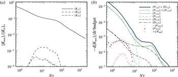
The influence of the stably stratified background on the three components of mean kinetic energy (MKE) is shown in figure 5(a). Histories of the (cross-domain) area-integrated quantities
 $\{K_{{\it\alpha}{\it\alpha}}\}=\{\overline{u}_{{\it\alpha}}\overline{u}_{{\it\alpha}}/2\}$
(
 ${\approx}4{\rm\pi}h_{y}h_{z}\langle \overline{u}_{{\it\alpha}}\overline{u}_{{\it\alpha}}/2\rangle$
) for
 ${\it\alpha}=1,2,3$
(no sum on
 ${\it\alpha}$
) are presented. Only during the NEQ regime are the lateral and vertical energies non-negligible compared with the streamwise component, and even then remain at least 1.5 orders of magnitude smaller than
 $\{K_{11}\}$
at all times. Nevertheless, all three components reveal discernible buoyancy effects. These can be deduced from figure 5(b), which presents histories of the dominant terms in the integrated MKE transport equation:
 $$\begin{eqnarray}\frac{\text{d}\{K_{{\it\alpha}{\it\alpha}}\}}{\text{d}t}=-\{P_{{\it\alpha}{\it\alpha}jj}\}-\{D_{{\it\alpha}{\it\alpha}jj}\}+\{B_{{\it\alpha}{\it\alpha}}\},\quad {\it\alpha}=(1,2,3),\end{eqnarray}$$
where
 $$\begin{eqnarray}\displaystyle -P_{{\it\alpha}{\it\alpha}jj}=\overline{u_{{\it\alpha}}^{\prime }u_{j}^{\prime }}\frac{\partial \overline{u}_{{\it\alpha}}}{\partial x_{j}} & & \displaystyle\end{eqnarray}$$
is the mean-to-turbulence transfer term (i.e. the negative rate of TKE production),
 $$\begin{eqnarray}\displaystyle D_{{\it\alpha}{\it\alpha}jj}={\it\nu}\frac{\partial \overline{u}_{{\it\alpha}}}{\partial x_{j}}\frac{\partial \overline{u}_{{\it\alpha}}}{\partial x_{j}} & & \displaystyle\end{eqnarray}$$
is the mean dissipation rate and
 $$\begin{eqnarray}\displaystyle B_{{\it\alpha}{\it\alpha}}=-g\overline{{\it\rho}}\,\overline{u}_{{\it\alpha}}{\it\delta}_{{\it\alpha}3}/{\it\rho}_{\infty }=\mathscr{B}_{mke}=-g\overline{{\it\rho}}\,\overline{w}/{\it\rho}_{\infty } & & \displaystyle\end{eqnarray}$$
is the mean buoyancy transfer (which appears with opposite sign in the transport equation for the mean potential energy
 $(g\overline{{\it\rho}}\,\overline{{\it\rho}}/2)/{\it\rho}_{\infty }|{\it\Gamma}|$
). It should be noted that the integrals of both the advection
 $A_{{\it\alpha}{\it\alpha}jj}=-\overline{u}_{j}\partial K_{{\it\alpha}{\it\alpha}}/\partial x_{j}$
and flux divergence/transfer
 $T_{{\it\alpha}{\it\alpha}jj}=-\partial \overline{u}_{{\it\alpha}}\overline{u_{{\it\alpha}}^{\prime }u_{j}^{\prime }}/\partial x_{j}+{\it\nu}\partial [\overline{u}_{{\it\alpha}}\partial \overline{u}_{{\it\alpha}}/\partial x_{j}]/\partial x_{j}$
terms are zero,
 $\{A_{{\it\alpha}{\it\alpha}jj}\}=\{T_{{\it\alpha}{\it\alpha}jj}\}=0$
. For the present flow, for which
 $\partial \overline{(\phantom{x})}/\partial x_{1}=\partial \overline{(\phantom{x})}/\partial x=0$
,
 $-P_{{\it\alpha}{\it\alpha}jj}=-P_{{\it\alpha}{\it\alpha}22}-P_{{\it\alpha}{\it\alpha}33}$
and
 $D_{{\it\alpha}{\it\alpha}jj}=D_{{\it\alpha}{\it\alpha}22}+D_{{\it\alpha}{\it\alpha}33}$
.
Regarding the
 $K_{11}$
balance, the end of the 3D period is first evident in the dissipation terms
 $\{D_{1122}\}$
and
 $\{D_{1133}\}$
, in that the mean vertical gradients enhanced by the vertical flattening of the wake overwhelm the lateral variations, thereby arresting the reduction of
 $\{D_{1133}\}$
(compare the single- and double-dot-dashed curves in figure 5
b). This begins near
 $N{\it\tau}=1.5$
; however, the dissipation terms are too small, relative to the TKE production, to have a controlling influence on the
 $\{K_{11}\}$
history. Shortly thereafter, at
 $N{\it\tau}\approx 2.5$
(when the
 $U_{d}$
history first departs from the
 ${\it\tau}^{-2/3}$
interpolant for the 3D regime; see figure 1
b), the curvature in the
 $\{K_{11}\}$
history changes, as a result of near-identical reductions of
 $\{P_{1122}\}$
and
 $\{P_{1133}\}$
, the MKE-to-TKE transfer terms respectively associated with the lateral
 $-\overline{u^{\prime }v^{\prime }}$
and vertical
 $-\overline{u^{\prime }w^{\prime }}$
shear stresses. Buoyancy has begun to affect the structure of the turbulence, such that
 $-\overline{u^{\prime }w^{\prime }}$
becomes a smaller and smaller fraction of the TKE for
 $N{\it\tau}>2.5$
, while
 $-\overline{u^{\prime }v^{\prime }}/k$
remains nearly constant until well into the NEQ regime (see figure 10
b). (We shall see below (figures 10
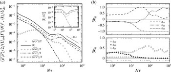
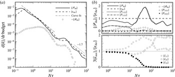
a and 11) that the TKE begins to increase its rate of decay
 $|\{\text{d}k/\text{d}t\}|$
near
 $N{\it\tau}=2.5$
, as the result of weakening TKE production and growing buoyancy transfer (acting as a TKE sink), relative to the local rate of TKE dissipation.) Combined with buoyancy-induced alterations of the mean flow – which reduce (compared with the unstratified counterpart) the lateral shear
 $\partial \overline{u}/\partial y$
and enhance the vertical shear
 $\partial \overline{u}/\partial z$
(see § 3.5 and figure 6) – this leads to the comparable reductions of
 $-P_{1122}=\overline{u^{\prime }v^{\prime }}\partial \overline{u}/\partial y$
and
 $-P_{1133}=\overline{u^{\prime }w^{\prime }}\partial \overline{u}/\partial z$
seen in figure 5(b) (see also figure 11
b). The result is a less rapid decay of
 $\{K_{11}\}$
(and presumably
 $U_{d}$
), as the MKE-to-TKE transfer is diminished, as the wake enters its NEQ phase.
At
 $N{\it\tau}\approx 5.5$
, the time at which the 3D and NEQ interpolants for
 $U_{d}$
intersect (figure 1
b), figure 5(b) implies that the processes begun at
 $N{\it\tau}\approx 2.5$
carry on unabated, until
 $N{\it\tau}\approx 9$
(somewhat after the time,
 $N{\it\tau}\approx 6.5$
, at which the
 $U_{d}$
history first begins to track with the NEQ interpolant; figure 1
b), when the buoyancy drives the vertical velocity fluctuations, and thus
 $P_{1133}$
, to zero, leaving
 $P_{1122}$
(after
 $N{\it\tau}\approx 15$
) to account for all the MKE-to-TKE transfer from the streamwise component. (Recall that for this flow the nominal duration of the NEQ regime, based on the times at which the 3D, NEQ and Q2D power-law interpolants for
 $U_{d}$
intersect, is
 $5.5<N{\it\tau}<45$
, while its ‘formal’ duration, based on the period when
 $U_{d}$
tracks closely with the
 ${\it\tau}^{-0.25}$
interpolant, is
 $6.5<N{\it\tau}<30$
.) Dommermuth et al. (Reference Dommermuth, Rottman, Innis and Novikov2002) and Brucker & Sarkar (Reference Brucker and Sarkar2010) have highlighted the correlation between vanishing
 $P_{1133}$
and the occurrence of the NEQ regime; the present results indicate that its inception is triggered by a joint reduction of
 $P_{1122}$
and
 $P_{1133}$
, which begins near
 $N{\it\tau}=2.5$
. We note that the
 $P_{1122}$
and
 $P_{1133}$
histories do not deviate from each other until after the magnitude
 $U_{d}$
and especially the height
 $h_{z}$
of the mean defect begin to display characteristics associated with NEQ behaviour (figures 1
b and 2
a), and that this (
 $N{\it\tau}\approx 9$
) deviation is not only the result of the rapid reduction of
 $P_{1133}$
, but also a consequence of
 $P_{1122}$
beginning to ‘wake up’ at approximately the same time (which mitigates the
 $|\text{d}U_{d}/\text{d}t|$
reduction). The attenuation of the rate of decay (and eventual change of sign, between
 $N{\it\tau}\approx 25$
and
 $60$
) of
 $\text{d}\{P_{1122}\}/\text{d}t$
can be attributed to another buoyancy-forced alteration of the turbulence structure, such that the magnitude of the lateral shear stress (figure 10
b) becomes large enough to overcome the reduction in the mean lateral shear
 $\partial \overline{u}/\partial y$
and thus produces enhanced
 $P_{1122}$
.
By the time
 $U_{d}$
departs from the
 ${\it\tau}^{-1/4}$
NEQ interpolant, near
 $N{\it\tau}=30$
(figure 1
b), the rate of decay of the streamwise MKE,
 $\text{d}\{K_{11}\}/\text{d}t$
, has returned to levels comparable to its pre-NEQ value. This increase is initially due to comparable contributions from the lateral MKE-to-TKE transfer
 $P_{1122}$
and vertical gradient dissipation
 $D_{1133}$
. The ‘bump’ observed in the
 $\{K_{11}\}$
history between
 $N{\it\tau}\approx 25$
and
 $100$
(see also the
 $U_{d}$
history over this range, in figure 1
b) corresponds to the period of
 $P_{1122}$
enhancement, during which
 $\{P_{1122}\}/\{D_{1133}\}>1$
, bridging the NEQ-to-Q2D transition. (We shall see in § 3.6 that this period includes the time,
 $25<N{\it\tau}<90$
, over which the net rate of TKE production exceeds that of net TKE dissipation; see figure 11.) The slowing of the decay of
 $P_{1122}$
appears to be an integral part of the NEQ regime, with its amplification marking the time at which the wake begins to move towards its Q2D phase. For
 $N{\it\tau}>150$
or so, the differences between the lateral TKE production (which has begun to fall again) and vertical gradient dissipation are statistically insignificant.
The
 $\{K_{11}\}$
history thus reflects alterations to both the mean flow (increased
 $\partial \overline{u}/\partial z$
, amplifying the mean dissipation and modulating the MKE-to-TKE transfer; decreased
 $\partial \overline{u}/\partial y$
, also modulating the MKE-to-TKE transfer) and turbulence (reduced
 $-\overline{u^{\prime }w^{\prime }}$
and enhanced
 $-\overline{u^{\prime }v^{\prime }}$
, respectively throttling and augmenting the MKE-to-TKE transfer terms
 $P_{1133}$
and
 $P_{1122}$
). Two further effects of buoyancy can be observed in the vertical and lateral components of the MKE budget. The first is direct transfer via net positive
 $\mathscr{B}_{mke}=-g\overline{{\it\rho}}\,\overline{w}/{\it\rho}_{\infty }$
, which supplies energy from the MPE to the vertical component (open diamonds in figure 5(b), which for illustration purposes trace positive
 $\{\mathscr{B}_{mke}\}$
on the
 $-\text{d}\{K_{33}\}/\text{d}t$
plot). It should be noted, however, that in terms of its effect on the mean defect (since
 $\mathscr{B}_{mke}$
is not a direct source of
 $K_{11}$
), this can be viewed solely as a symptom of the mean flow collapse,
 $\partial \overline{w}/\partial z<0$
, associated with the indirect/modulating influences cited above.
The second further buoyancy effect visible in the non-
 $K_{11}$
budgets in figure 5 is manifested by another alteration of the TKE production terms, again due to negative
 $\partial \overline{w}/\partial z<0$
and (due to continuity) lateral expansion (
 $\partial \overline{v}/\partial y>0$
) of the mean flow in the wake core, such that
 $-P_{3333}=\overline{w^{\prime }w^{\prime }}\partial \overline{w}/\partial z<0$
and
 $-P_{2222}=\overline{v^{\prime }v^{\prime }}\partial \overline{v}/\partial v>0$
. The latter ‘anti-TKE-production’ is responsible for the growth of
 $\{K_{22}\}$
, the former mitigating the increase in
 $\{K_{33}\}$
caused by
 $\{\mathscr{B}_{mke}\}$
, such that
 $\{K_{33}\}$
remains much smaller than
 $\{K_{22}\}$
. (Although
 $P_{2222}$
is a net sink of TKE during the NEQ regime, it is not an important one, as can be seen in figure 11
b of § 3.6;
 $P_{3333}$
is also insignificant, except within the
 $40<N{\it\tau}<100$
range, when it acts as a TKE source, with a magnitude of a few per cent of the TKE dissipation rate.)
Having catalogued the above buoyancy effects, the question now arises of how they combine to modify the maximum velocity and
 $y$
–
 $z$
spatial structure of the mean defect (i.e.
 $U_{d}$
,
 $h_{z}$
and
 $h_{y}$
) during the 3D, NEQ and Q2D regimes. To address this question, we turn our attention to the budget of mean streamwise momentum.
3.5. Reynolds-averaged Navier–Stokes budget
For the present time-dependent parallel flow the streamwise Reynolds-averaged Navier–Stokes (RANS) equation can be written as
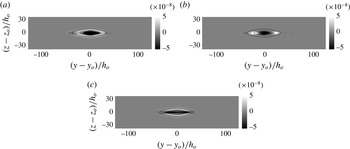
 $$\begin{eqnarray}\frac{\partial \overline{u}}{\partial t}=\underbrace{\left(-\overline{v}\frac{\partial \overline{u}}{\partial y}-\overline{w}\frac{\partial \overline{u}}{\partial z}\right)}_{\text{advection}}+\underbrace{\left(-\frac{\partial \overline{u^{\prime }v^{\prime }}}{\partial y}-\frac{\partial \overline{u^{\prime }w^{\prime }}}{\partial z}\right)}_{\text{Reynolds\text{-}stress divergence}}+\underbrace{{\it\nu}\left(\frac{\partial ^{2}\overline{u}}{\partial y^{2}}+\frac{\partial ^{2}\overline{u}}{\partial z^{2}}\right)}_{\text{viscous\text{-}stress divergence}}.\end{eqnarray}$$
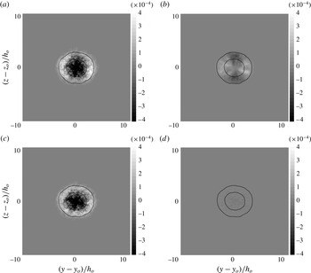
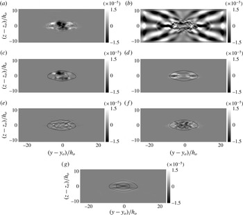
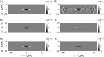
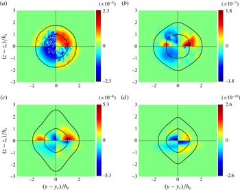
Contours of the net rate of change of mean velocity
 $\partial \overline{u}/\partial t$
and the terms that contribute to it are shown in figures 6–9. The closed solid-line curves on each panel correspond to locations at which
 $\overline{u}/U_{d}=0.05$
and
 $0.5$
, and thus indicate the extent of the mean defect (with the mean height
 $h_{z}$
and width
 $h_{y}$
defined respectively by the points at which the inner,
 $\overline{u}=0.5U_{d}$
, curve crosses the
 $z$
- and
 $x$
-axes).
Terms in the mean streamwise momentum budget at
 $N{\it\tau}=2.5$
: (a) rate of change
 $\partial \overline{u}/\partial t$
; (b) advection
 $-\overline{v}\partial \overline{u}/\partial y-\overline{w}\partial \overline{u}/\partial z$
; (c) Reynolds-stress divergence
 $-\partial \overline{u^{\prime }v^{\prime }}/\partial y-\partial \overline{u^{\prime }w^{\prime }}/\partial z$
; (d) viscous-stress divergence
 ${\it\nu}(\partial ^{2}\overline{u}/\partial y^{2}+\partial ^{2}\overline{u}/\partial z^{2})$
. The size and shape of the mean defect are indicated by closed solid-line curves, which denote
 $\overline{u}=0.05U_{d}$
and
 $0.5U_{d}$
. Budget terms are given in units of
 $U_{r}^{2}/L_{r}$
, where
 $U_{r}=2.09U_{do}$
and
 $L_{r}=h_{o}$
.

During the 3D phase, the reduction in
 $U_{d}$
and increase in the wake height and width – i.e. the negative
 $\partial \overline{u}/\partial t$
near the centreline and the positive
 $\partial \overline{u}/\partial t$
at the wake edge – are driven by the divergence of the Reynolds stress,
 $-\partial \overline{u^{\prime }v^{\prime }}/\partial y-\partial \overline{u^{\prime }w^{\prime }}/\partial z$
. This can be inferred from figure 6, which shows the cross-wake-plane distribution of
 $\partial \overline{u}/\partial t$
and how the advection, turbulence and viscous terms contribute to it at
 $N{\it\tau}=2.5$
, as the effects of buoyancy first begin to appear. At this time, the Reynolds-stress divergence near the centreline has been slightly weakened, due to reduced
 $-\overline{u^{\prime }w^{\prime }}$
and widening of the region over which
 $-\overline{u^{\prime }w^{\prime }}$
is distributed (recall the discussion above regarding change in behaviour of the streamwise MKE for
 $N{\it\tau}\approx 2.5$
) and the axisymmetric/3D nature of the flow slightly altered by the buoyancy, as the flow moves towards the NEQ regime. Although the relative strengths of the vertical and lateral components of the Reynolds-stress divergence remain comparable at the edges of the wake, the flattening and widening of the region of wake turbulence caused by the buoyant forcing is apparent. This is a consequence of the buoyancy-induced mean ‘vertical stagnation’ flow,
 $\partial \overline{w}/\partial z=-\partial \overline{v}/\partial y<0$
, nominally centred at the wake centreline, leading to (i) negative vertical advection,
 $-\overline{w}\partial \overline{u}/\partial z$
, above and below the centreline (dark regions in figure 6
b), and thus reduced rate of vertical spreading; (ii) positive lateral advection,
 $-\overline{v}\partial \overline{u}/\partial y$
, at the left and right of the defect (light regions in figure 6
b), and therefore enhanced lateral spreading. The fact that the near-axis region is dominated by the Reynolds-stress distribution, which has yet to be significantly modified, while the mean advection is most prominent at the wake edges, helps to explain the earlier observation that
 $h_{z}$
and
 $h_{y}$
depart from 3D behaviour before
 $U_{d}$
does.
Terms in the mean streamwise momentum budget at
 $N{\it\tau}=18$
(NEQ regime): (a) rate of change
 $\partial \overline{u}/\partial t$
; (b)
 $-\partial \overline{u}\,\overline{w}/\partial z$
; (c) vertical advection
 $-\overline{w}\partial \overline{u}/\partial z$
; (d) lateral advection
 $-\overline{v}\partial \overline{u}/\partial y$
; (e) vertical Reynolds-stress divergence
 $-\partial \overline{u^{\prime }w^{\prime }}/\partial z$
; (f) lateral Reynolds-stress divergence
 $-\partial \overline{u^{\prime }v^{\prime }}/\partial y$
; (g) vertical viscous-stress divergence
 ${\it\nu}\partial ^{2}\overline{u}/\partial z^{2}$
. The size and shape of the mean defect are indicated by closed solid-line curves, which denote
 $\overline{u}=0.05U_{d}$
and
 $0.5U_{d}$
. Budget terms are given in units of
 $U_{r}^{2}/L_{r}$
.

Within the NEQ regime the story is more complex. Significant internal-wave activity, in the
 ${\it\kappa}_{x}=0$
(i.e. streamwise mean) mode, is generated by the wake, revealed by the vertical mean momentum flux divergence,
 $-\partial \overline{u}\,\overline{w}/\partial z$
(figure 7
b, for
 $N{\it\tau}=18$
). However, the waves do not make a meaningful contribution to the net momentum (or the kinetic energy), since
 $-\partial \overline{u}\,\overline{w}/\partial z-\partial \overline{u}\,\overline{v}/\partial y\equiv -\overline{w}\partial \overline{u}/\partial z-\overline{v}\partial \overline{u}/\partial y$
is essentially zero outside the wake (figure 7
c,d). Figure 7(a,c) also shows that at
 $N{\it\tau}=18$
, when
 $\text{d}h_{z}/\text{d}t\approx \text{d}r_{z}^{\ast }/\text{d}t\approx 0$
, the regions at the top and bottom of the wake are affected even more strongly than at
 $N{\it\tau}=2.5$
by the mean vertical stagnation. In fact, the negative vertical advection, due to the negative
 $\partial \overline{w}/\partial z$
along the
 $z$
axis, is now so large compared with the other terms that nearly no trace remains of positive
 $\partial \overline{u}/\partial t$
above and below the wake. The effect of the lateral advection is also important, although now qualitatively different from its
 $N{\it\tau}=2.5$
contribution, due to a fundamental change in the
 $\overline{v}$
–
 $\overline{w}$
mean flow near the centreline. At
 $N{\it\tau}=2.5$
, it forms a simple stagnation pattern centred about the wake centreline, with vertical inflow along the vertical axis and lateral outflow along the horizontal axis. On the other hand, figure 7(d) implies that at
 $N{\it\tau}=18$
, the stagnation pattern contains both vertical and lateral inflow, along their respective axes, while the outflow streamlines are now ‘deflected’ above and below the
 $y$
axis, such that
 $-\overline{v}\partial \overline{u}/\partial y$
now (like the vertical advection) acts as a momentum sink at the sides of the wake. The resulting dual-peak pattern in the lateral advection distribution is similar to that seen in the
 $y$
–
 $z$
contours of TKE at this time (see figure 8c of Redford et al.
Reference Redford, Lund and Coleman2014). The negative-
 $\partial \overline{u}/\partial t$
contribution at the sides of the wake (at
 $z=0$
) provided by the lateral advection (in contrast to its positive values at
 $N{\it\tau}=2.5$
, seen in figure 6
b), is consistent with the reduction of the rate of change of the mean width,
 $\text{d}h_{y}/\text{d}t$
, for the NEQ regime (figure 2
b).
The (slower, compared with the 3D state) rate of decrease of
 $U_{d}(t)$
at
 $N{\it\tau}=18$
is primarily the result of the lateral Reynolds-stress divergence
 $-\partial \overline{u^{\prime }v^{\prime }}/\partial y$
. As seen above, both Reynolds stresses, but especially the vertical component
 $-\overline{u^{\prime }w^{\prime }}$
, are profoundly affected by the buoyancy (which drives
 $w^{\prime }\rightarrow 0$
, such that
 $-\overline{u^{\prime }w^{\prime }}$
goes to zero faster in the NEQ regime than the growth of the lateral component
 $-\overline{u^{\prime }v^{\prime }}$
can overcome; see figure 10
b). The result is that the importance of the Reynolds-shear-stress divergence, especially the vertical component, has been reduced to levels comparable to that of the vertical viscous stresses (contrast figure 7
e–g). (The lateral stress is now a somewhat larger fraction of the TKE, whose rate of decay is slowing, than it was before stratification altered the turbulence (figure 10
b), but the increase is mitigated by the lateral spreading of the defect, such that
 $-\partial \overline{u^{\prime }v^{\prime }}/\partial y$
is not as large as it would be if
 $\text{d}h_{y}/\text{d}t=0$
.) The increasing importance of viscous effects within the NEQ regime is through the vertical viscous term (which tends to mirror and counteract the ‘deflected-outflow’ stagnation pattern of the lateral advection); it reveals a ‘flattened-hourglass’ arrangement of the streamwise mean velocity not observable in the vertical
 $\overline{u}(z,y_{c})$
and lateral
 $\overline{u}(z_{c},y)$
profiles in figure 3. The lateral viscous-stress divergence (not shown) remains negligible.
Terms in the mean streamwise momentum budget at
 $N{\it\tau}=82$
(Q2D regime): (a) rate of change
 $\partial \overline{u}/\partial t$
; (b)
 $-\partial \overline{u}\,\overline{w}/\partial z$
; (c) vertical advection
 $-\overline{w}\partial \overline{u}/\partial z$
; (d) lateral advection
 $-\overline{v}\partial \overline{u}/\partial y$
; (e) lateral Reynolds-stress divergence
 $-\partial \overline{u^{\prime }v^{\prime }}/\partial y$
; (f) vertical viscous-stress divergence
 ${\it\nu}\partial ^{2}\overline{u}/\partial z^{2}$
. The size and shape of the mean defect are indicated by closed solid-line curves, which denote
 $\overline{u}=0.05U_{d}$
and
 $0.5U_{d}$
. Budget terms are given in units of
 $U_{r}^{2}/L_{r}$
. The vertical Reynolds-stress divergence
 $-\partial \overline{u^{\prime }w^{\prime }}/\partial z$
and lateral viscous-stress divergence
 ${\it\nu}\partial ^{2}\overline{u}/\partial y^{2}$
are negligible compared with the terms shown.

The difference between the
 $\partial \overline{u}\,\overline{w}/\partial z$
contours in figures 7(b) (
 $N{\it\tau}=18$
) and 8(b) (
 $N{\it\tau}=82$
) displays the tendency for the strength of the internal waves to fade as the wake passes from the NEQ to the Q2D regime. For the present flow the strongest internal-wave activity occurs towards the start of the NEQ phase. The spatial scales imply that the waves are generated by individual turbulence structures – rather than, say, collapse of the mean defect associated with entry into the Q2D regime. A thorough computational study of internal-wave radiation by stably stratified wakes at various Froude and Reynolds numbers has been performed recently by Abdilghanie & Diamessis (Reference Abdilghanie and Diamessis2013).
Once the Q2D phase has begun, the core deceleration is dominated by the lateral Reynolds-stress divergence, and to a lesser extent by the vertical advection and vertical viscous-stress terms. This can be seen in the
 $N{\it\tau}=82$
results in figure 8(e,c,f). The vertical Reynolds-stress
 $-\partial \overline{u^{\prime }w^{\prime }}/\partial z$
and lateral viscous-stress
 ${\it\nu}\partial ^{2}\overline{u}/\partial y^{2}$
divergences are now negligible. At the top and bottom edges of the wake, the vertical viscous-stress divergence is now solely responsible for the small net positive
 $\partial \overline{u}/\partial t$
here – a fact foreshadowed by the
 ${\it\tau}^{1/2}$
growth of the mean height observed in figure 2(a). In contrast, the (faster) lateral spreading is due to the lateral advection (figure 8
d) and especially the lateral Reynolds-stress term (figure 8
e), with the former focused near
 $\pm h_{y}$
, the latter farther out, just inside the
 $0.05U_{d}$
contour. We also note that the multilayered structure seen in visualizations of turbulence in the NEQ range (e.g. figure 5 of Redford et al.
Reference Redford, Lund and Coleman2014) has now matured to the point that it affects the RANS budget, leaving its signature in the terms involving spatial gradients of the mean velocity, such as
 $-\overline{v}\partial \overline{u}/\partial y$
(figure 8
d). This term indicates that the
 $\overline{v},\overline{w}$
mean flow has reverted to its original ‘simple’ vertical-collapse stagnation pattern, first observed at
 $N{\it\tau}=2.5$
, with the mean lateral outflow again along the
 $\pm y$
axis. The ‘extra peaky’ vertical profile of
 $\overline{u}(y_{0},z)$
observed at this time (dash-single-dot curve in figure 3
a) can be traced to the negligible
 $\partial \overline{u}/\partial t$
at the top and bottom of the wake. (Recall the slightly negative
 $\text{d}h_{z}/\text{d}t$
at this time, shown in figure 2
a.)
Terms in the mean streamwise momentum budget at
 $N{\it\tau}=586$
(late Q2D regime): (a) rate of change
 $\partial \overline{u}/\partial t$
; (b) lateral Reynolds-stress divergence
 $-\partial \overline{u^{\prime }v^{\prime }}/\partial y$
; (c) vertical viscous-stress divergence
 ${\it\nu}\partial ^{2}\overline{u}/\partial z^{2}$
. The size and shape of the mean defect are indicated by closed solid-line curves, which denote
 $\overline{u}=0.05U_{d}$
and
 $0.5U_{d}$
. Budget terms are given in units of
 $U_{r}^{2}/L_{r}$
. The mean vertical momentum divergence
 $-\partial \overline{u}\,\overline{w}/\partial z$
, advection
 $-\overline{v}\partial \overline{u}/\partial y-\overline{w}\partial \overline{u}/\partial z$
, vertical Reynolds-stress divergence
 $-\partial \overline{u^{\prime }w^{\prime }}/\partial z$
and lateral viscous-stress divergence
 ${\it\nu}\partial ^{2}\overline{u}/\partial y^{2}$
are negligible compared with the terms shown.

As time passes, the importance of the
 $-\partial \overline{u^{\prime }v^{\prime }}/\partial y$
and
 ${\it\nu}\partial ^{2}\overline{u}/\partial z^{2}$
terms continues to grow relative to the other ones, until they are the only significant contributors to the RANS budget (cf. Meunier et al.
Reference Meunier, Diamessis and Spedding2006) (and, as shown above,
 $P_{1122}$
and
 $D_{1133}$
are the only significant contributors to the streamwise MKE budget; figure 5
b). At
 $N{\it\tau}=586$
(figure 9), both terms decelerate the centreline region by approximately the same amount, but have very different effects on the spreading of the defect: the mean acceleration at the top and bottom of the defect caused by the viscous diffusion is much weaker than that produced at the sides by the lateral divergence of the
 $-\overline{u^{\prime }v^{\prime }}$
Reynolds stress, induced by the Q2D regime’s pancake-eddy turbulence (see figure 6 of Redford et al.
Reference Redford, Lund and Coleman2014). (The slight lateral asymmetry of the
 $-\partial \overline{u^{\prime }v^{\prime }}/\partial y$
contours in figure 9(b) is a statistical anomaly, due to the relatively small number of eddy structures included in the streamwise average at this time.) The decoupling of the viscous (vertical) and turbulent (lateral) mixing mechanisms during the late Q2D regime is consistent with the disparate rates of vertical and lateral spreading observed in figure 2, with
 ${\it\beta}_{y}$
larger than
 ${\it\beta}_{z}$
for
 $N{\it\tau}>100$
, and the earlier observation that the growth of
 $h_{z}$
is a purely viscous phenomenon during this time (Meunier et al.
Reference Meunier, Diamessis and Spedding2006).
To summarize this section, we recount the stratification effects revealed by the RANS budgets. For
 $U_{d}$
, the onset of the NEQ regime is triggered by weakening of both the lateral and especially the vertical Reynolds-stress divergence, the former because
 $-\overline{u^{\prime }v^{\prime }}$
falls and is distributed over a wider lateral extent, as a consequence of stable buoyancy widening the mean defect, the latter because of reduced
 $-\overline{u^{\prime }w^{\prime }}$
(as
 $w^{\prime }\rightarrow 0$
). The lateral Reynolds stress begins to intensify within the NEQ regime, due to the buoyancy-forced change of the turbulence structure, which eventually results in the energetic pancake eddies associated with the Q2D phase, and thereby the large
 $-\partial \overline{u^{\prime }v^{\prime }}/\partial y$
responsible for the enhanced decay of
 $U_{d}$
in the late wake. The mean flow flattening influence of the buoyancy also produces significant mean vertical viscous-stress divergence in the late-Q2D regime.
The stable stratification affects the mean defect height
 $h_{z}$
primarily through mean vertical collapse
 $\partial \overline{w}/\partial z<0$
near the centreline, which during the entrance to the NEQ regime slows
 $\text{d}h_{z}/\text{d}t$
by way of vertical advection of the mean streamwise velocity. The slower
 $\text{d}h_{z}/\text{d}t$
during the Q2D phase is a consequence of buoyancy removing all vertical spreading except that due to the vertical viscous-stress divergence,
 ${\it\nu}\partial ^{2}\overline{u}/\partial z^{2}$
.
The mean width history is also correlated with the mean flow pattern induced by the buoyancy, in particular the lateral outflow
 $\partial \overline{v}/\partial y$
along the
 $y$
axis: when
 $\partial \overline{v}/\partial y$
is positive (as it is during both the late-3D/early-NEQ and early-Q2D regimes), lateral advection,
 $-\overline{v}\partial \overline{u}/\partial y$
, represents a source of
 $\text{d}h_{y}/\text{d}t$
; when
 $\partial \overline{v}/\partial y$
is negative along the
 $y$
axis and the mean outflow from the centreline has a vertical component (see figure 7
d, for
 $N{\it\tau}=18$
),
 $\text{d}h_{y}/\text{d}t$
is reduced. As the wake moves deeper into the Q2D regime, the effect of the stratification on the turbulence structure (and therefore on the lateral Reynolds-stress divergence) becomes increasingly significant, until (when the lateral advection becomes negligible) it alone is responsible for the enhanced
 $\text{d}h_{y}/\text{d}t$
.
To further clarify the role of buoyancy in the turbulent-wake dynamics, we now examine the behaviour of the turbulence kinetic energy and the terms in its budget.
3.6. Turbulence kinetic energy history and budget
Figure 10(a) shows the manner in which stratification alters the cross-wake-averaged potential and kinetic energy of the turbulence,
 $(g\langle \overline{{\it\rho}^{\prime }{\it\rho}^{\prime }}\rangle /2)/{\it\rho}_{\infty }|{\it\Gamma}|$
(symbols) and
 $\langle k\rangle =\langle \overline{u_{i}^{\prime }u_{i}^{\prime }}\rangle /2$
(lines) respectively. (Recall that the cross-wake average is over regions where
 $\overline{u}\geqslant 0.05U_{d}$
.)
Histories of (a) the cross-wake-averaged turbulence potential and kinetic energy and (b) the Reynolds-stress anisotropy
 $\unicode[STIX]{x1D623}_{ij}=\langle |\overline{u_{i}^{\prime }u_{j}^{\prime }}|\rangle /2\langle k\rangle -{\it\delta}_{ij}/3$
. The inset plot in (a) shows components scaled by local
 $U_{d}$
.

The density fluctuations are largest early in the NEQ regime, when buoyancy most strongly affects the flow and the internal waves are most active. The present case, with its large initial Froude number (
 $Fr_{\infty }\approx 130$
), does not contain the buoyancy-induced temporal oscillations of TKE observed at early times in Dommermuth et al.’s (Reference Dommermuth, Rottman, Innis and Novikov2002)
 $Fr_{\infty }=4$
LES and Brucker & Sarkar’s (Reference Brucker and Sarkar2010)
 $Fr_{\infty }=8$
DNS, for which
 $\text{d}k/\text{d}t$
first becomes positive near
 $Nt\approx N{\it\tau}=5.5$
for the former and
 $N{\it\tau}=2.3$
for the latter (see figure 13 below regarding the value of the virtual origin
 $Nt_{vo}$
used for the Brucker & Sarkar simulation). Those oscillations, which are damped more slowly in the lower
 $Fr_{\infty }$
flow, are indicative of transfer back and forth between the potential and kinetic energy of the turbulence, associated with changes in sign of the TKE-to-TPE exchange term,
 $\mathscr{B}_{tke}=-g\overline{{\it\rho}^{\prime }w^{\prime }}/{\it\rho}_{\infty }$
(Brucker & Sarkar mention, but do not quantify, ‘large values of the buoyancy flux at early time’). For the present flow, we shall soon see that
 $\mathscr{B}_{tke}$
always acts as a net sink of TKE, despite the monotonic decrease with time of the local mean Froude number
 $Fr_{d}$
(figure 12
a,b).
Instead of increasing towards the beginning of the NEQ regime, here the TKE increases for
 $30<N{\it\tau}<70$
, i.e. during the NEQ-to-Q2D transition defined by the
 $U_{d}$
history (figure 1
b). The reasons for this increase, which is unrelated to the TPE-to-TKE transfer via
 $\mathscr{B}_{tke}$
, will soon be clear.
The difference between the rates of decay of the three velocity fluctuations, as well as the non-constant variation of
 $\langle k\rangle /U_{d}^{2}$
for
 $N{\it\tau}>4$
(solid curve in figure 10
a inset), demonstrates the anisotropy introduced by the stratification, and how it breaks the early axisymmetry, leading to a flow for which the relationship between the magnitudes of the velocity fluctuations and the maximum mean defect continues to evolve throughout the NEQ and Q2D regimes. Of the three components, the streamwise TKE
 $\langle \overline{u^{\prime }u^{\prime }}\rangle /2$
(dashed curve) exhibits the least variation with respect to the local
 $U_{d}^{2}$
, but even so varies significantly (by over a factor of five) as the wake regimes come and go. For
 $N{\it\tau}>150$
, when the TKE is reasonably approximated by a
 ${\it\tau}^{-4/3}$
power law,
 $k$
decays more slowly than
 $U_{d}^{2}$
does, such that (assuming
 $U_{d}\sim {\it\tau}^{-0.85}$
in the Q2D range)
 $\langle k\rangle /U_{d}^{2}\sim {\it\tau}^{+0.37}$
(figure 10
a inset plot).
The disparate effect of the stratification upon the three velocity-fluctuation components, and thus on the structure of the Reynolds-stress tensor, can also be seen in figure 10(a,b). The Reynolds-stress-anisotropy
 $\unicode[STIX]{x1D623}_{ij}$
histories show that the velocity fluctuations first deviate from axisymmetric decay behaviour (i.e.
 $\overline{v^{\prime }v^{\prime }}\approx \overline{w^{\prime }w^{\prime }}$
and
 $\overline{u^{\prime }v^{\prime }}\approx \overline{u^{\prime }w^{\prime }}$
) near
 $N{\it\tau}=2$
, the time at which the mean defect height and width, and the mean vertical and lateral dissipation rates of the MKE, begin to differ from each other (figures 2 and 5
b). Thereafter, the vertical component falls monotonically, first slowly then rapidly, such that
 $\overline{w^{\prime }w^{\prime }}$
and both
 $\overline{u^{\prime }w^{\prime }}$
and
 $\overline{v^{\prime }w^{\prime }}$
are negligible for
 $N{\it\tau}>40$
(cf. Spedding Reference Spedding2002; Diamessis et al.
Reference Diamessis, Spedding and Domaradzki2011). The precipitous drop in the vertical velocity fluctuations means that buoyancy can no longer directly cause a transfer between the turbulence potential and kinetic energies (recall that
 $\mathscr{B}_{tke}=-g\overline{{\it\rho}^{\prime }w^{\prime }}/{\it\rho}_{\infty }$
).
The streamwise normal stress
 $\overline{u^{\prime }u^{\prime }}$
becomes an ever larger fraction of the
 $2k=\overline{u^{\prime }u^{\prime }}+\overline{v^{\prime }v^{\prime }}+\overline{w^{\prime }w^{\prime }}$
total until the flow is well within the NEQ regime, when
 $\text{d}\langle k\rangle /\text{d}t$
becomes positive, near
 $N{\it\tau}\approx 30$
. Afterwards, the normal component
 $\overline{v^{\prime }v^{\prime }}$
increases faster than
 $\overline{u^{\prime }u^{\prime }}$
, and
 $-\overline{u^{\prime }v^{\prime }}$
is the only significant shear stress. The dominance of
 $-\overline{u^{\prime }v^{\prime }}$
corresponds to that of the
 $P_{1122}$
production term in the TKE transport equation (cf. figure 5
b). During the
 $N{\it\tau}>70$
phase of the Q2D regime, when
 $\text{d}\langle k\rangle /\text{d}t$
is again negative (and the flow is dominated by pancake-eddy structures), the lateral fluctuations have more energy than the streamwise fluctuations do, with
 $\langle \overline{v^{\prime }v^{\prime }}\rangle /\langle \overline{u^{\prime }u^{\prime }}\rangle \rightarrow 2$
for
 $N{\it\tau}>400$
.
History of terms in the budget of the integrated TKE
 $\{k\}$
. Terms in (a) are given in units of
 $U_{r}^{3}L_{r}$
, those in (b) as a fraction of the local
 $\{{\it\epsilon}_{tke}\}$
. The interpolant in (a) (chain-double-dot curve) is given by
 $A_{{\it\epsilon}}(N{\it\tau})^{-5/3}=A_{{\it\epsilon}}(Nt-Nt_{vo})^{-5/3}$
, with
 $(A_{{\it\epsilon}},Nt_{vo})=(0.00138,0.645)$
. Production terms not shown are either zero because of homogeneity (
 $\{P_{1111}\}=\{P_{2211}\}=\{P_{3311}\}\equiv 0$
) or negligible (
 $\{P_{2233}\}\approx \{P_{3322}\}\approx 0$
). Components of dissipation rate
 $\tilde{{\it\epsilon}}_{{\it\alpha}{\it\alpha}}={\it\nu}\overline{(\partial u_{{\it\alpha}}^{\prime }/\partial x_{j})(\partial u_{{\it\alpha}}^{\prime }/\partial x_{j})}$
(no sum on
 ${\it\alpha}$
), where
 $\tilde{{\it\epsilon}}_{ii}={\it\epsilon}_{tke}-{\it\nu}\partial ^{2}\overline{u_{i}^{\prime }u_{j}^{\prime }}/\partial x_{i}\partial x_{j}$
, and
 ${\it\epsilon}_{tke}=2{\it\nu}\overline{s_{ij}^{\prime }s_{ij}^{\prime }}$
.

To further quantify these effects, we consider the TKE
 $k$
transport equation, which can be written as
 $$\begin{eqnarray}\frac{\partial k}{\partial t}=\mathscr{A}_{tke}+\mathscr{P}_{tke}+\mathscr{F}_{tke}+\mathscr{B}_{tke}-{\it\epsilon}_{tke}+\mathscr{W}_{tke},\end{eqnarray}$$
where the rates of change due to advection
 $\mathscr{A}_{tke}$
, production
 $\mathscr{P}_{tke}$
, flux divergence
 $\mathscr{F}_{tke}$
, buoyancy transport
 $\mathscr{B}_{tke}$
and dissipation
 ${\it\epsilon}_{tke}$
are, respectively,
 $\mathscr{A}_{tke}=-\overline{u}_{j}\partial k/\partial x_{j}$
,
 $\mathscr{P}_{tke}=P_{iijj}=-\overline{u_{i}^{\prime }u_{j}^{\prime }}\partial \overline{u}_{i}/\partial x_{j}$
,
 $\mathscr{F}_{tke}=\partial f_{j}/\partial x_{j}$
, with
 $f_{j}=-\overline{u_{j}^{\prime }u_{i}^{\prime }u_{i}^{\prime }}/2-\overline{u_{j}^{\prime }p^{\prime }}/{\it\rho}_{\infty }+{\it\nu}\partial \overline{u_{i}^{\prime }u_{j}^{\prime }}/\partial x_{i}+{\it\nu}\partial k/\partial x_{j}$
, and
 $\mathscr{B}_{tke}=-g\overline{{\it\rho}^{\prime }u_{i}^{\prime }}{\it\delta}_{i3}/{\it\rho}_{\infty }$
and
 ${\it\epsilon}_{tke}=2{\it\nu}\overline{s_{ij}^{\prime }s_{ij}^{\prime }}$
, with
 $s_{ij}^{\prime }=(\partial u_{i}^{\prime }/\partial x_{j}+\partial u_{j}^{\prime }/\partial x_{i})/2$
. For the flow at hand, these reduce to
 $\mathscr{A}_{tke}=-\overline{v}\partial k/\partial y-\overline{w}\partial k/\partial z$
,
 $\mathscr{P}_{tke}=P_{ii22}+P_{ii33}$
,
 $\mathscr{F}_{tke}=\partial [-\overline{v^{\prime }u_{i}^{\prime }u_{i}^{\prime }}/2-\overline{v^{\prime }p^{\prime }}/{\it\rho}_{\infty }+{\it\nu}\partial \overline{v^{\prime }v^{\prime }}/\partial y+{\it\nu}\partial \overline{v^{\prime }w^{\prime }}/\partial z+{\it\nu}\partial k/\partial y]/\partial y+\partial [-\overline{w^{\prime }u_{i}^{\prime }u_{i}^{\prime }}/2-\overline{w^{\prime }p^{\prime }}/{\it\rho}_{\infty }+{\it\nu}\partial \overline{v^{\prime }w^{\prime }}/\partial y+{\it\nu}\partial \overline{w^{\prime }w^{\prime }}/\partial z+{\it\nu}\partial k/\partial z]/\partial z$
and
 $\mathscr{B}_{tke}=-g\overline{{\it\rho}^{\prime }w^{\prime }}/{\it\rho}_{\infty }$
. The work done by the fringe forcing
 $F_{i}$
(see Redford et al.
Reference Redford, Lund and Coleman2014), corresponding to energy radiated to the far field by internal waves, is
 $\mathscr{W}_{tke}=\overline{u_{i}^{\prime }F_{i}}$
(
 $i=1,2,3$
).
Since the advection and flux-divergence terms integrate to zero, net TKE transfer is only effected by the production
 $\mathscr{P}_{tke}$
, dissipation
 ${\it\epsilon}_{tke}$
, TKE–TPE exchange
 $\mathscr{B}_{tke}$
and internal-wave radiation
 $\mathscr{W}_{tke}$
(i.e. items 1, 4, 5 and 6 respectively, in figure 4). For the present high-
 $Fr_{\infty }$
flow, the sum of the production, dissipation and buoyancy is sufficient to provide an excellent representation of the
 $\text{d}\{k\}/\text{d}t$
history, for
 $0\leqslant Nt<840$
(see figure 3b of Redford et al.
Reference Redford, Lund and Coleman2014), which implies that the fringe work contribution
 $\{\mathscr{W}_{tke}\}$
(and thus that of the internal waves) to the TKE balance is negligible. Figure 11 presents the cross-plane area-integrated histories of the non-negligible transfer terms in (3.6). The cross-plane variation of these terms, and
 $\mathscr{A}_{tke}(y,z)$
and
 $\mathscr{F}_{tke}(y,z)$
, is examined in appendix B. We note that the net buoyancy transfer
 $\{B_{tke}\}$
represents a pure sink of TKE at all times. This is the major result of this section.
3.6.1. Further TKE budget considerations
The buoyancy transfer is much smaller than the production and dissipation, but not insignificant, with
 $-\{\mathscr{B}_{tke}\}$
reaching a maximum of about 30 % of the integrated dissipation rate
 $\{{\it\epsilon}_{tke}\}$
from early in the NEQ regime (
 $N{\it\tau}\approx 5$
) and remaining fixed near this ratio until
 $N{\it\tau}\approx 60$
(figure 11
b); thereafter
 $-\{\mathscr{B}_{tke}\}$
is a monotonically decreasing fraction of
 $\{{\it\epsilon}_{tke}\}$
until it becomes negligible for
 $N{\it\tau}$
greater than approximately
 $150$
. Between
 $N{\it\tau}\approx 25$
and
 $70$
, all three non-negligible terms are roughly constant in absolute terms, with
 $\text{d}\{{\it\epsilon}_{tke}\}/\text{d}t$
and
 $\text{d}\{\mathscr{B}_{tke}\}/\text{d}t$
approximately zero and
 $\text{d}\{\mathscr{P}_{tke}\}/\text{d}t$
increasing slightly. Spedding (Reference Spedding2002) found a similar early Q2D plateau in the total dissipation
 ${\it\epsilon}_{tke}+{\it\nu}(\partial \overline{u}_{i}/\partial x_{j})(\partial \overline{u}_{i}/\partial x_{j})$
in his high-
 $Fr_{\infty }$
experiments, which he attributed to the dominance of vertical shear. Although the global/integrated buoyancy transfer
 $\{\mathscr{B}_{tke}\}$
acts as a net sink of TKE throughout the lifetime of the present flow, there are times where there are small local regions in which
 $\mathscr{B}_{tke}$
is positive, where the potential energy of the turbulence is converted to kinetic energy (see figure 17 of Redford et al.
Reference Redford, Lund and Coleman2014). During the early-NEQ phase, these tend to be concentrated just above and below the wake, while later they are more diffuse and disorganized, although still occurring mostly outside the wake core.
Figure 11(a) shows that the Reynolds number is large enough for the early/3D regime evolution to satisfy the inertial scaling
 ${\it\epsilon}_{tke}\sim k^{3/2}/h$
, such that
 ${\it\epsilon}_{tke}\sim {\it\tau}^{-7/3}$
and
 $\{{\it\epsilon}_{tke}\}\sim {\it\tau}^{-5/3}$
(chain-double-dot curve; cf. Brucker & Sarkar Reference Brucker and Sarkar2010). For late times,
 $N{\it\tau}>200$
or so, the decay of
 $\{\mathscr{P}_{tke}\}$
and especially
 $\{{\it\epsilon}_{tke}\}$
is reasonably well approximated by
 ${\it\tau}^{-n}$
with
 $n=1.7\approx 5/3$
. Thus, paradoxically, the TKE dissipation evolves according to the inertial scaling during both the 3D and Q2D regimes, despite their qualitatively different eddy structures (see figure 17
d).
The beginning of the exit from the 3D regime observed near
 $N{\it\tau}=2.5$
in the
 $U_{d}$
and MKE histories (figures 1
b and 5
a), which coincides with the start of a period of increased TKE decay (figure 10
a), can be traced to the reduced relative importance, with respect to the rate of dissipation, of TKE production, as well as the growing importance of the TKE-to-TPE transport via buoyancy (figure 11). Once the wake turbulence is fully established, the net rate of TKE dissipation is larger than that of the production
 $\mathscr{P}_{tke}$
, except for a substantial period that bridges the end of the NEQ and start of the Q2D regime, from
 $N{\it\tau}\approx 25$
to
 $90$
, when
 $\{\mathscr{P}_{tke}\}$
is as much as 90 % larger than
 $\{{\it\epsilon}_{tke}\}$
(and, from
 $N{\it\tau}\approx 25$
to
 $55$
, gradually increases, in absolute terms), after which it returns to its pre-NEQ behaviour, in that
 $\{\mathscr{P}_{tke}\}/\{{\it\epsilon}_{tke}\}<1$
for the Q2D phase. This explains the growth of TKE during this period. From figure 11(b) we find that the enhanced production is due solely to amplification of the
 $P_{1122}=-\overline{u^{\prime }v^{\prime }}\partial \overline{u}/\partial y$
component (dotted curve), since the
 $-\overline{u^{\prime }v^{\prime }}$
stress grows more rapidly than
 $\partial \overline{u}/\partial y$
decreases (and the fall of
 $-\overline{u^{\prime }w^{\prime }}$
is more rapid than the attenuation of the decay of
 $\partial \overline{u}/\partial z$
). This ‘structural’ alteration, represented by the decrease of
 $-\overline{u^{\prime }w^{\prime }}$
and increase of
 $-\overline{u^{\prime }v^{\prime }}$
, was also found by Brucker & Sarkar (Reference Brucker and Sarkar2010) in their DNS, for both towed and self-propelled cases. They concluded that stratification causes the TKE production to mainly consist of
 $P_{1122}$
during this time. The present results emphasize the extent to which this is also true for this flow, for which
 $\mathscr{P}_{tke}$
can effectively be replaced by
 $P_{1122}$
for all times after
 $N{\it\tau}\approx 15$
.
While both the present and Brucker & Sarkar simulations contain enhanced production, only here does it lead to growth of TKE (and not just reduction in the net TKE decay) during the end of the NEQ regime. This is because of the large amount of energy radiated by internal waves between
 $N{\it\tau}=25$
and
 $75$
in Brucker & Sarkar’s
 $Fr_{\infty }=8$
flow, which counteracts the impact of the
 $P_{1122}$
growth (see also Dommermuth et al.
Reference Dommermuth, Rottman, Innis and Novikov2002). The strength of the internal waves is an indication of when the TKE growth occurs. When they are strong, at low
 $Fr_{\infty }$
, buoyancy leads to an early TKE increase driven by the TPE-to-TKE transfer, before the NEQ regime begins – during which the energy radiated by the waves mitigates the effect of the enhanced TKE production associated with the flattened two-layer NEQ/Q2D structure, and
 $\text{d}\{k\}/\text{d}t$
is small but negative. When the waves are weak, at high
 $Fr_{\infty }$
, they do not attenuate the enhanced
 $\mathscr{P}_{tke}\approx P_{1122}$
, leading to net TKE growth, which signals the end of the NEQ regime.
Also included in figure 11(b) are histories of the three components of the integrated rate of homogeneous dissipation,
 $\{\tilde{{\it\epsilon}}_{ii}\}=\{\tilde{{\it\epsilon}}_{11}\}+\{\tilde{{\it\epsilon}}_{22}\}+\{\tilde{{\it\epsilon}}_{33}\}$
, as a fraction of the full (actual thermodynamic) rate of TKE dissipation
 $\{{\it\epsilon}_{tke}\}=2{\it\nu}\{\overline{s_{ij}^{\prime }s_{ij}^{\prime }}\}$
, where
 $\tilde{{\it\epsilon}}_{ii}={\it\nu}\overline{(\partial u_{i}^{\prime }/\partial x_{j})(\partial u_{i}^{\prime }/\partial x_{j})}$
. (There is very little difference between the integrated homogeneous and full/inhomogeneous dissipation for this flow, with
 $0.9999965\leqslant \{\tilde{{\it\epsilon}}_{ii}\}/\{{\it\epsilon}_{tke}\}\leqslant 1.0012$
throughout the simulation.) Examination of
 $\tilde{{\it\epsilon}}_{{\it\alpha}{\it\alpha}}$
for
 ${\it\alpha}=1,2,3$
allows one to assess the interplay between the rates of production and dissipation of the individual normal-stress components
 $\overline{u_{{\it\alpha}}^{\prime }u_{{\it\alpha}}^{\prime }}$
. (Other dissipation decompositions have been utilized by Spedding (Reference Spedding2002) and Brucker & Sarkar (Reference Brucker and Sarkar2010); see also Itsweire et al. (Reference Itsweire, Koseff, Briggs and Ferziger1993).)
The vertical component
 $\{\tilde{{\it\epsilon}}_{33}\}\sim \{(\partial w^{\prime }/\partial x)^{2}\}+\{(\partial w^{\prime }/\partial y)^{2}\}+\{(\partial w^{\prime }/\partial z)^{2}\}$
falls monotonically as
 $w^{\prime }$
does, with
 $\text{d}\{\tilde{{\it\epsilon}}_{33}\}/\text{d}t$
becoming negative from
 $N{\it\tau}\approx 7$
until
 $N{\it\tau}>50$
or so, when
 $\{\tilde{{\it\epsilon}}_{33}\}$
is negligible with respect to
 $\{{\it\epsilon}_{tke}\}$
. For the streamwise component, the increase in
 $P_{1122}$
for
 $N{\it\tau}>5$
is accompanied by an increase in
 $\{\tilde{{\it\epsilon}}_{11}\}$
, such that the net effect (to which the pressure–strain correlation
 ${\it\phi}_{11}=\overline{p^{\prime }(\partial u^{\prime }/\partial x)}/{\it\rho}_{\infty }$
may also contribute) is to arrest the decay of
 $\overline{u^{\prime }u^{\prime }}$
, such that
 $\text{d}\{\overline{u^{\prime }u^{\prime }}\}/\text{d}t$
first changes sign and then becomes slightly positive for
 $N{\it\tau}>20$
(figure 10
a). This is an example of what is often referred to as an ‘extra strain’ effect (Bradshaw Reference Bradshaw1988), which involves a difficult-to-model change that results from the imbalance of much larger terms of opposite sign, each of which changes much more than the net imbalance. Similar behaviour is found in the Q2D regime, in that as
 $\text{d}\{\overline{u^{\prime }u^{\prime }}\}/\text{d}t$
becomes negative again, both
 $\{P_{1122}\}$
and
 $\{\tilde{{\it\epsilon}}_{11}\}$
decrease (the latter accounting for roughly one-third of the total
 $\{{\it\epsilon}_{tke}\}$
).
The evolution of the lateral component
 $\overline{v^{\prime }v^{\prime }}$
during the 3D-to-NEQ transition is not directly affected by production (since
 $P_{2211}\equiv 0$
and
 $P_{2222}\approx P_{2233}\approx 0$
). Consequently, the slight increase in
 $\{\overline{v^{\prime }v^{\prime }}\}$
between
 $N{\it\tau}\approx 25$
and
 $80$
shown in figure 10(a) must be due to intercomponent transfer by way of the pressure-strain term
 ${\it\phi}_{22}=\overline{p^{\prime }(\partial v^{\prime }/\partial y)}/{\it\rho}_{\infty }$
, reduced somewhat by
 $\{\tilde{{\it\epsilon}}_{22}\}$
, which first falls slightly below
 $\{{\it\epsilon}_{tke}\}/3$
(i.e. the isotropic value approximated by all three components before
 $N{\it\tau}\approx 5$
), then grows to account for approximately
 $2/3$
of the total.
The dissipation histories are broadly consistent with those observed in Brucker & Sarkar’s (Reference Brucker and Sarkar2010) low-
 $Fr_{\infty }$
/self-propelled wake simulation, in that
 $\overline{(\partial u^{\prime }/\partial z)^{2}}$
and
 $\overline{(\partial v^{\prime }/\partial z)^{2}}$
(i.e. the dominant terms in
 $\tilde{{\it\epsilon}}_{11}$
and
 $\tilde{{\it\epsilon}}_{22}$
respectively) are respectively the second-largest and largest terms for
 $N{\it\tau}>10$
(although the contributions of
 $\partial v^{\prime }/\partial x$
,
 $\partial w^{\prime }/\partial x$
and
 $\partial w^{\prime }/\partial z$
were not quantified, these are likely to be negligible). The
 $\{\tilde{{\it\epsilon}}_{{\it\alpha}{\it\alpha}}\}$
histories are thus also consistent with the enhanced vertical gradients associated with the flattened eddy structures of the NEQ and Q2D regimes (see figures 5 and 6 of Redford et al.
Reference Redford, Lund and Coleman2014).
Further information regarding the TKE budget is presented in appendix B, where the 2D cross-wake variation of the individual terms for the 3D, NEQ and Q2D regimes is documented. This illustrates, in particular, the importance of the flux-divergence transport terms (which integrate to zero over the
 $y$
–
 $z$
plane, and therefore do not appear in the integrated balances considered above) in the evolution of the spatial variation of the rate of change of the TKE across the wake.
3.7. Comparison with previous simulations
The variations of the mean-defect-based Froude and Reynolds numbers for the present and earlier simulations (summarized in table 1) are shown in figure 12, defined in terms of both the wake’s mean height
 $h_{z}$
and width
 $h_{y}$
. Evidence of each of the 3D, NEQ and Q2D regimes can be seen. The tendency for all the Froude numbers to fall monotonically indicates that all the flows, even those with very large
 $Fr_{do}$
, eventually are dominated by buoyancy effects. The anisotropy introduced by the stable stratification is revealed by the differences between the Froude and Reynolds numbers based on
 $h_{z}$
and
 $h_{y}$
. The wake evolution is such that the power-law decay of the height-based Reynolds number
 $U_{d}h_{z}/{\it\nu}$
varies little over the life of the flow, while
 $U_{d}h_{y}/{\it\nu}$
remains relatively constant, especially during the NEQ phase (cf. Diamessis et al.
Reference Diamessis, Spedding and Domaradzki2011).
Summary of comparison cases.

a
The nominal Reynolds number of Diamessis et al.’s (Reference Diamessis, Spedding and Domaradzki2011) implicit LES is
 $V_{\infty }D/{\it\nu}=100\times 10^{3}$
, and
 $U_{do}h_{o}/{\it\nu}\approx 11\times 10^{3}$
.
The time required (
 $t\approx 1/N$
) for the vortex-ring initialization (solid line) to produce a fully turbulent state is apparent, which can be contrasted with the approaches used to define the
 $Nt=0$
state for the other simulations (recall the difficulties involved in specifying finite disturbances typical of the fully developed wake downstream of a sphere). The question of appropriate virtual origins, needed when comparing the present and earlier cases, will be taken up below.
Histories of mean (a,b) Froude number
 $Fr_{d}=U_{d}/Nh$
and (c,d) Reynolds number
 $Re_{d}=U_{d}h/{\it\nu}$
for the present and previous simulations (see table 1).

For Gourlay et al. (Reference Gourlay, Arendt, Fritts and Werne2001),
 $Fr_{do}=34.0$
and
 $Re_{do}=1472$
. The more recent simulations tended to use lower
 $Fr$
and higher
 $Re$
: Brucker & Sarkar’s (Reference Brucker and Sarkar2010) case TR50F
 $_{\infty }$
08 (i.e.
 $Fr_{\infty }=2V_{\infty }/ND=8$
,
 $Re_{\infty }=50\,000$
) corresponds to
 $Fr_{do}\approx 0.75$
and
 $Re_{do}\approx 3250$
(they assume
 $U_{do}/V_{\infty }=0.11$
and
 $D\approx 1.7h_{o}$
). (To avoid confusion associated with the different Froude number definitions used by Brucker & Sarkar (Reference Brucker and Sarkar2010) and Diamessis et al. (Reference Diamessis, Spedding and Domaradzki2011), which differ by a factor of two, and to allow direct comparison, the case names from these two studies have been modified as shown in table 1.) Brucker & Sarkar (Reference Brucker and Sarkar2010) also simulated a lower-
 $Re$
, higher-
 $Fr$
flow with which we will compare (case ‘TR10F
 $_{\infty }$
40’), with
 $(Fr_{do},Re_{do})\approx (3.75,650)$
. Comparison will also be made with the recent
 $Fr_{\infty }=64$
(
 $Fr_{do}\approx 14.5$
),
 $Re_{\infty }=10^{5}$
(
 $Re_{do}\approx 1.1\times 10^{4}$
) LES of Diamessis et al. (Reference Diamessis, Spedding and Domaradzki2011), for which the eddy-resolving capability was comparable to the present DNS. In fact, although the smallest resolved scales are not those that actually appear at
 $Re_{\infty }=10^{5}$
, the LES has the advantage of taking full benefit of the available spatial resolution – since the magnitude of the subgrid-scale viscosity of the LES can be smaller than the molecular viscosity of the DNS – and thus has the capacity to capture scales smaller than those of an over-resolved DNS at smaller Reynolds number, such as is used here.
Histories of (a) the maximum velocity
 $U_{d}$
, (b) the height-to-width ratio
 $\ell _{z}/\ell _{y}$
, (c) the height
 $\ell _{z}$
and (d) the width
 $\ell _{y}$
of the mean defect for the present and previous simulations (see table 1). The maximum defect velocity
 $U_{d}$
in (a) for Brucker & Sarkar’s (Reference Brucker and Sarkar2010) case TR50F
 $_{\infty }$
08 (but not TR10F
 $_{\infty }$
40) is replaced by their
 $U_{1}^{mke}$
. Integral measures are used for the height and width for the present DNS, with
 $\ell _{z}=r_{z}^{\ast }$
,
 $\ell _{y}=r_{y}^{\ast }$
, and
 $\ell _{o}$
the value of
 $r_{z}^{\ast }=r_{y}^{\ast }$
at
 $Nt=0$
. For Brucker & Sarkar’s (Reference Brucker and Sarkar2010) case TR50F
 $_{\infty }$
08,
 $\ell _{z}$
and
 $\ell _{y}$
are respectively represented by integral scales (in their notation)
 $R_{3}$
and
 $R_{2}$
, with
 $\ell _{o}$
the half-radius of the initial Gaussian mean velocity profile, while for Diamessis et al. (Reference Diamessis, Spedding and Domaradzki2011), and effectively for Gourlay et al. (Reference Gourlay, Arendt, Fritts and Werne2001),
 $\ell _{z}=h_{z}$
,
 $\ell _{y}=h_{y}$
and
 $\ell _{o}=h_{o}$
, where
 $h_{z}$
and
 $h_{y}$
are determined from fitting an assumed Gaussian profile. The inset plots show unstratified similarity diagnostics for (a) the velocity
 ${\it\chi}=(U_{d}/U_{do})^{-3/2}$
and (b) the height
 ${\it\xi}_{z}=(\ell _{z}/\ell _{o})^{3}$
(lower curve/symbols) and width
 ${\it\xi}_{y}=(\ell _{y}/\ell _{o})^{3}$
(upper curve/symbols); these are used to define the virtual time origin
 $t_{vo}$
for each case:
 $Nt_{vo}=0.645$
for the present DNS,
 $Nt_{vo}=0.2$
for Brucker & Sarkar’s TR50F
 $_{\infty }$
08,
 $Nt_{vo}=-0.5$
for Diamessis et al. and
 $Nt_{vo}=0$
for Gourlay et al. and Brucker & Sarkar’s TR10F
 $_{\infty }$
40. For the present DNS, the linear curve fits for
 ${\it\chi}$
and
 ${\it\xi}$
(thin solid lines) are
 ${\it\chi}=(U_{d}/U_{do})^{-3/2}=BN{\it\tau}$
and
 ${\it\xi}=(r^{\ast }/r_{o}^{\ast })^{3}=CN{\it\tau}$
, where
 $N{\it\tau}=Nt-Nt_{vo}$
and
 $(B,C,Nt_{vo})=(3.1,2.9,0.645)$
.

Figure 13 shows the mean defect histories from earlier simulations at various Froude and Reynolds numbers, along with the present results. Also shown are the unstratified/3D regime power-law diagnostics
 ${\it\chi}$
and
 ${\it\xi}$
for each case (inset plots in figure 13
a,b). These are used to estimate virtual time origins
 $t_{vo}$
for each simulation, to facilitate comparison of their histories (plotting versus
 $N{\it\tau}=Nt-Nt_{vo}$
), by associating
 $t_{vo}$
with the zero-crossing time of the (linear)
 $U_{d}^{-3/2}$
interpolant.
The various histories cannot be expected to agree in the scaling used for figure 13, which takes no account of Froude and/or Reynolds numbers, since the maximum velocities
 $U_{d}$
, heights
 $\ell _{z}$
and widths
 $\ell _{y}$
are presented solely in terms of their initial values. (Moreover,
 $\ell _{z}$
is for some cases given in terms of the
 $0.5U_{d}$
half-height
 $h_{z}$
and for others in terms of integral measures; see the caption to figure 13.) Nevertheless, several common features can be observed, including similar power-law behaviour over the same
 $N{\it\tau}$
range. The height decreases with time for
 $N{\it\tau}>2$
in every case, although the reduction of
 $h_{z}$
is larger than that experienced by the integral-measure heights (which is consistent with the behaviour found for the present DNS, in that both
 $\text{d}h_{z}/\text{d}t$
and
 $\text{d}r_{z}^{\ast }/\text{d}t$
are negative for
 $8<N{\it\tau}<18$
, but
 $h_{z}$
falls faster than
 $r_{z}^{\ast }$
; figure 2
a).
The 3D-to-NEQ transition also tends to occur at approximately the same time for each of the simulations, with
 $N{\it\tau}$
between
 $2$
and
 $2.5$
being the point at which the heights and widths first begin to differ from each other; this can be seen in figure 13(b) in the height-to-width ratio
 $\ell _{z}/\ell _{y}$
and is even more obvious in the unstratified/axisymmetric height/width diagnostic
 ${\it\xi}=(\ell /\ell _{o})^{3}$
shown in the inset plots (recall that linear variation with time of
 ${\it\xi}$
is characteristic of the pure axisymmetric 3D regime).
The reasonably good collapse of the mean aspect ratio
 $\ell _{z}/\ell _{y}$
over the early-NEQ periods of the five simulations was not anticipated, because of both the wide Froude- and Reynolds-number ranges, and the differences in the initialization strategies used for the various simulations (e.g. Brucker & Sarkar’s (Reference Brucker and Sarkar2010) DNS held the mean velocity fixed until
 $Nt=0.2$
(TR10F
 $_{\infty }$
40) and
 $1$
(TR50F
 $_{\infty }$
08), while Diamessis et al.’s (Reference Diamessis, Spedding and Domaradzki2011) LES gradually introduced the background stratification during a precursor simulation). The
 $\ell _{z}/\ell _{y}$
histories demonstrate the increase of the
 $N{\it\tau}$
range of the NEQ regime with Reynolds number predicted by Meunier et al. (Reference Meunier, Diamessis and Spedding2006) and observed by Diamessis et al. (Reference Diamessis, Spedding and Domaradzki2011): compare the times at which the
 $\ell _{z}/\ell _{y}$
histories begin to deviate from the negative power-law behaviour for NEQ, for Brucker & Sarkar’s (Reference Brucker and Sarkar2010) TR10F
 $_{\infty }$
40 (
 $40<N{\it\tau}<100$
), Gourlay et al. (Reference Gourlay, Arendt, Fritts and Werne2001) (
 $N{\it\tau}\approx 70$
), present (
 $N{\it\tau}\approx 105$
) and Brucker & Sarkar’s (Reference Brucker and Sarkar2010) TR50F
 $_{\infty }$
08 (
 $N{\it\tau}>400$
, at least). (The late-time
 $\ell _{z}/\ell _{y}$
history for Diamessis et al. (Reference Diamessis, Spedding and Domaradzki2011) (open diamonds) is thought to be statistically unreliable, in light of the relatively small streamwise domain used.) The same message regarding the Reynolds-number dependence of the NEQ period can be inferred from figure 13(c), by examining the durations of the
 $\text{d}\ell _{z}/\text{d}t\approx 0$
regions for each case.
The tendency for
 $\ell _{z}$
and
 $\ell _{y}$
to deviate from the 3D/axisymmetric ideal sooner than
 $U_{d}$
does, which was observed above, also holds for the other simulations (although not as markedly), since the unstratified/axisymmetric similarity diagnostic for
 $U_{d}$
,
 ${\it\chi}=(U_{d}/U_{do})^{-3/2}$
, remains linear for longer (until
 $N{\it\tau}\approx 2$
to
 $5$
) than the corresponding height/width diagnostic,
 ${\it\xi}$
(
 $N{\it\tau}\approx 2$
to
 $2.5$
); cf. figure 13(a,b) inset plots.
A scaling to account for the significant Froude-number sensitivity of the
 $U_{d}$
histories seen in figure 13(a) has been developed by Meunier & Spedding (Reference Meunier and Spedding2004). It amounts to assuming that
 $U_{d}$
will eventually depend solely on the volume-flux deficit
 $I_{d}$
, the Brunt–Väisälä frequency
 $N$
and time
 $t$
, which leads via dimensional analysis to
 $$\begin{eqnarray}\frac{U_{d}}{(I_{d}N^{2})^{1/3}}={\it\Phi}(Nt-Nt_{0}),\end{eqnarray}$$
where
 ${\it\Phi}$
is a universal non-dimensional function of
 $Nt-Nt_{0}$
and
 $Nt_{0}$
is a non-universal offset time (unrelated to the 3D virtual origin
 $Nt_{vo}$
), which will depend, for example, on the Reynolds number and the near-field/early-wake evolution. In terms of a virtual wake-creating sphere of diameter
 $D$
immersed in a steady uniform stream of density
 ${\it\rho}_{\infty }$
and speed
 $V_{\infty }$
, experiencing a drag force
 $F_{D}$
, we can write
 $I_{d}=V_{\infty }D^{2}C_{D}/8$
, where
 $C_{D}=F_{D}/({\rm\pi}{\it\rho}_{\infty }V_{\infty }^{2}D^{2}/8)$
. Equation (3.7) then implies
 $$\begin{eqnarray}\frac{U_{d}}{V_{\infty }}Fr_{\infty }^{2/3}=f(C_{D}){\it\Phi}(Nt-Nt_{0}),\end{eqnarray}$$
where
 $f(C_{D})=({\rm\pi}C_{D}/2)^{1/3}$
. Equation (3.8) shows the limitation of attempting to collapse
 $U_{d}/V_{\infty }$
data from wakes generated by various bluff bodies (with variable
 $C_{D}$
) by using only
 $Fr_{\infty }$
(e.g. by plotting
 $(U_{d}/V_{\infty })Fr_{\infty }^{2/3}$
versus
 $Nt$
; cf. Spedding (Reference Spedding1997), Brucker & Sarkar (Reference Brucker and Sarkar2010)). Following Meunier & Spedding (Reference Meunier and Spedding2004), (3.7) can be recast in terms of the virtual effective diameter
 $D_{eff}=D(C_{D}/2)^{1/2}$
for bluff bodies of arbitrary shape,
 $$\begin{eqnarray}\frac{U_{d}}{V_{\infty }}Fr_{eff}^{2/3}={\rm\pi}^{1/3}{\it\Phi}(Nt-Nt_{0}),\end{eqnarray}$$
where
 $Fr_{eff}=2V_{\infty }/ND_{eff}$
is the effective Froude number.
Histories of the rescaled mean defect (a,c) as a Q2D power-law/similarity diagnostic and (b,d) with respect to the Q2D time shift
 $Nt_{0}$
, assuming (a,b)
 $n=3/4$
and (c,d)
 $n=0.85$
, for the present and previous simulations (see table 1). The thin solid curves in (a,c) are linear curve fits of the Q2D diagnostic (which for Gourlay et al. (Reference Gourlay, Arendt, Fritts and Werne2001) and case TR10F
 $_{\infty }$
40 of Brucker & Sarkar (Reference Brucker and Sarkar2010) are nearly coincident), used to define the time shift
 $Nt_{0}$
in (b,d), such that for (b) (
 $n=3/4$
)
 $Nt_{0}=:19$
(present DNS),
 $-55$
(Gourlay et al.
Reference Gourlay, Arendt, Fritts and Werne2001),
 $-63.5$
(Brucker & Sarkar’s (Reference Brucker and Sarkar2010) case TR50F
 $_{\infty }$
08),
 $-57$
(Brucker & Sarkar’s (Reference Brucker and Sarkar2010) case TR10F
 $_{\infty }$
40) and
 $11$
(Diamessis et al.’s (Reference Diamessis, Spedding and Domaradzki2011) case R100F
 $_{\infty }$
64), and for (d) (
 $n=0.85$
)
 $Nt_{0}=:7$
(present DNS),
 $-70$
(Gourlay et al.
Reference Gourlay, Arendt, Fritts and Werne2001),
 $-66.5$
(Brucker & Sarkar’s (Reference Brucker and Sarkar2010) case TR50F
 $_{\infty }$
08),
 $-71$
(Brucker & Sarkar’s (Reference Brucker and Sarkar2010) case TR10F
 $_{\infty }$
40) and
 $-3$
(Diamessis et al.’s (Reference Diamessis, Spedding and Domaradzki2011) case R100F
 $_{\infty }$
64).

The validity of (3.7) is tested in figure 14. Meunier & Spedding (Reference Meunier and Spedding2004) found that the universality under consideration cannot be expected until the flow reaches the Q2D regime (see their figure 5b). Consequently, we assume
 ${\it\Phi}(Nt-Nt_{0})=C_{Q2D}(Nt-Nt_{0})^{-n}$
, where
 $C_{Q2D}$
is a universal constant and
 $n\approx 3/4$
. Similar slopes of the
 $(U_{d}/I_{d}^{1/3}N^{2/3})^{-1/n}$
diagnostic are found for all five simulations, for both
 $n=3/4$
(figure 14
a, with
 $C_{Q2D}=0.08^{-3/4}\approx 6.65$
) and the
 $n=0.85$
suggested by the present DNS (figure 14
c;
 $C_{Q2D}=0.055^{-0.85}\approx 11.8$
). One should note the dependence of the beginning of the region of common slope (straight thin solid lines in figure 14
a,c) and the offset times
 $Nt_{0}$
(
 $Nt$
-axis intercept) on the Reynolds number and initialization scheme used by each simulation. The reasonable agreement of the results in figure 14(b,d), produced by using the
 $Nt_{0}$
defined for each case by the corresponding curve fits in figure 14(a,c), points to the validity of (3.7), which implies that the founding assumptions used in the Meunier & Spedding (Reference Meunier and Spedding2004) analysis are sound. It also contributes to the body of evidence supporting the universality of late-wake behaviour in stably stratified media.
4. Summary and closing comments
The DNS results presented here reveal the effect of a weakly stratified buoyantly stable background upon the structure and statistics of a turbulent wake, during various phases of development, including the 3D, NEQ and Q2D regimes. This has been documented by the evolution of the mean kinetic energy, mean momentum and turbulence kinetic energy, and the terms in their budgets. The present study underlines the importance of adequate ‘eddy sample’ (by way of sufficient streamwise domain size) in order to reduce the uncertainty associated with use of time-developing simulations.
The power-law variations that best fit the present results, for the 3D (
 $t^{p}$
), NEQ (
 $t^{m}$
) and Q2D (
 $t^{n}$
) regimes, are
 $(p,m,n)=(-2/3,-1/4,-0.85)$
for
 $U_{d}$
, (
 $+1/3$
,
 ${\approx}0,+0.5$
) for
 $h_{z}$
and
 $(+1/3,+1/8,+0.35)$
for
 $h_{y}$
. We should perhaps also reiterate that the NEQ and Q2D histories could be adequately fitted with somewhat different power-law exponents when combined with different virtual origins. The power-law behaviour implied by other simulations can be inferred from figure 13.
The present results demonstrate that the reduction in the rate of TKE decay associated with the NEQ regime need not be accompanied by transfer from the gravitational potential energy of the turbulence to the kinetic energy of the turbulence. This potential-to-kinetic-energy (‘restratification’) mechanism (which does appear for lower-Froude-number cases, when the TKE–TPE exchange term exhibits temporal oscillations; see Dommermuth et al. (Reference Dommermuth, Rottman, Innis and Novikov2002) and Brucker & Sarkar (Reference Brucker and Sarkar2010)) is thus apparently not the fundamental cause of the 3D-to-NEQ transition. Instead, we find that the TKE enhancement is due to increased production effected by the buoyancy forcing the turbulence to become increasingly two-dimensional, such that the
 $-\overline{u^{\prime }v^{\prime }}$
lateral Reynolds shear stress dominates (see also Brucker & Sarkar Reference Brucker and Sarkar2010). However, since it is the reduction in the rate of decrease of the maximum mean defect velocity
 $|\text{d}U_{d}/\text{d}t|$
(not
 $|\text{d}k/\text{d}t|$
) that first signals the presence of the NEQ regime (and the present mean defect behaviour agrees well with that seen at other Froude and Reynolds numbers; cf. figure 13), a case could be made that it is the processes that alter the mean streamwise velocity (rather than the TKE) that are fundamental to the 3D-to-NEQ conversion. Whether the TKE increase is best understood as the ‘official arrival’ of the NEQ regime, or the beginning of the NEQ-to-Q2D transition (see below), is a question that requires further study, at Reynolds numbers higher than the one we have considered. The mean kinetic energy and mean momentum budgets indicate that the buoyancy-induced suppression of
 $|\text{d}U_{d}/\text{d}t|$
at the end of the 3D phase is again due to alterations of the turbulence structure; however, these are manifested through weakened lateral and especially vertical Reynolds-stress divergence (rather than the enhanced lateral Reynolds stress and thus TKE production). Unlike the TKE enhancement, the
 $|\text{d}U_{d}/\text{d}t|$
alteration is accompanied by potential-to-kinetic-energy transfer, in the sense that
 $|\text{d}U_{d}/\text{d}t|$
is affected by the vertical collapse of the mean flow (i.e.
 $\partial \overline{w}/\partial z<0$
), through changing (e.g. vertically decreasing) the area over which the Reynolds stresses are distributed, and thus influencing their divergence (i.e. their contribution to
 $\partial \overline{u}/\partial t$
) in the wake core. The mean vertical collapse also impacts the growth of the mean defect height and width, via advection of
 $\overline{u}$
at the wake edges.
For the present high-
 $Fr_{\infty }$
case, internal-wave activity is most pronounced at the start of the NEQ regime. However, even during this time, internal waves make a negligible contribution to the turbulence energy and mean momentum budgets. This is in contrast to the strongly stratified cases studied elsewhere, for which the amount of turbulence energy radiated by internal waves during the NEQ regime can be comparable to that produced by the mean shear or lost by way of viscous dissipation (cf. Brucker & Sarkar Reference Brucker and Sarkar2010).
Structural alterations are also responsible for the transition from the NEQ to the Q2D regime, in that the ‘two-dimensionalization’ of the turbulence by the buoyancy leads to flattened coherent energetic eddies swirling in
 $x$
–
 $y$
planes, which cause the lateral Reynolds stress
 $-\overline{u^{\prime }v^{\prime }}$
, in conjunction with viscous fluxes that pass down steep mean vertical gradients of velocity, to define the flow evolution (Spedding Reference Spedding2001; Meunier & Spedding Reference Meunier and Spedding2004; Brucker & Sarkar Reference Brucker and Sarkar2010). The enhanced
 $-\overline{u^{\prime }v^{\prime }}$
(whose growth relative to the TKE begins within the NEQ regime) is responsible for a surplus of TKE production, which for the present high-
 $Fr_{\infty }$
case (since losses associated with radiation of internal waves are negligible) causes a net growth of TKE,
 $\text{d}k/\text{d}t>0$
. Surprisingly, despite their structural differences, the TKE dissipation decays at approximately the same rate during the early/3D and late/Q2D regimes. This affirms the dissimilarity between the Q2D state and pure 2D turbulence (cf. Godeford & Cambon Reference Godeford and Cambon1994).
The role of stable stratification in driving the wake towards a universal state has also been displayed, in that the late-time evolution of the mean wake characteristics is independent of the details of the (here, vortex-ring) wake initialization (a fact frequently observed in other experiments and simulations). Comparison of results from the present and previous simulations illustrates that, in units of
 $N^{-1}$
, the duration of the NEQ regime increases with the Reynolds number, as predicted by Meunier et al. (Reference Meunier, Diamessis and Spedding2006), and observed by Brucker & Sarkar (Reference Brucker and Sarkar2010) and Diamessis et al. (Reference Diamessis, Spedding and Domaradzki2011). This comparison also indicates that during the Q2D regime, the history of the maximum mean defect
 $U_{d}$
(appropriately normalized, in terms of the initial volume-flux deficit
 $I_{d}$
(set by the speed, size and drag coefficient of the wake-creating body) and the Brunt–Väisälä frequency
 $N$
) is a unique function of non-dimensional time
 $Nt$
(relative to a flow-dependent virtual offset/origin). This supports the validity of the framework proposed by Meunier & Spedding (Reference Meunier and Spedding2004) in their universal model of the mean defect evolution for a stably stratified towed wake.
Acknowledgements
This project was supported by the Revolutionary Computational AeroSciences project under NASA’s Fundamental Aerodynamics programme, by the UK Ministry of Defence (Dstl project RD027-02854, managed by Dr R. P. Hornby) and by the UK Turbulence Consortium, funded by the UK Engineering and Physical Sciences Research Council (EPSRC), under Grants EP/D044073/1 and EP/G069581/1. It made use of the facilities of HPCx and HECToR, the UK’s National High-performance Computing Service, which is provided by UoE HPCx Ltd at the University of Edinburgh, Cray Inc. and NAG Ltd, and funded by the Office of Science and Technology through EPSRC’s High End Computing Programme. We are grateful to Dr S. L. Woodruff for reviewing the manuscript and to the referees for a number of helpful suggestions.
Histories of the mean defect velocity
 $U_{d}$
, width
 $h_{y}$
and height
 $h_{z}$
for simulations with different streamwise domain sizes
 ${\it\Lambda}_{x}$
. Histories are shown with respect to virtual offset times
 $t_{vo}$
defined by each simulation’s unstratified similarity diagnostic
 ${\it\xi}$
(see figure 13), and normalized by their value at
 $N{\it\tau}=1$
.

Appendix A. Effect of streamwise domain size and time step on mean defect history
The relationship between the sample size and the uncertainty of the mean defect statistics was examined by comparing results from simulations that are identical except for the size of the streamwise domain
 ${\it\Lambda}_{x}$
. Three cases were considered, with
 ${\it\Lambda}_{x}/h_{o}=32{\rm\pi}$
,
 $64{\rm\pi}$
and
 $96{\rm\pi}$
, the latter being the value used to generate the data presented above. The resulting defect histories are shown in figure 15. To account for the slight differences in the initial conditions for each case (caused by the fact that each simulation is initialized by a different number of vortex rings and that each ring is subjected to different random perturbations), the
 $U_{d}$
,
 $h_{y}$
and
 $h_{z}$
histories for each run are plotted with respect to the virtual origin
 $t_{vo}$
defined by their
 $U_{d}$
variation in the 3D regime, and normalized by their value at
 $Nt-Nt_{vo}=1$
. The tendency for the means to diverge with time is clear, as is the reduction of the magnitude of the statistical oscillations with increasing
 ${\it\Lambda}_{x}$
(corresponding to larger streamwise sample size), especially for the width and height measures. These findings suggest that the defect histories from the
 ${\it\Lambda}_{x}/h_{o}=96{\rm\pi}$
simulation discussed in § 3 are not significantly affected by statistical uncertainty until at least the end of the NEQ regime.
The negligible effect of temporal discretization error on the mean defect evolution is demonstrated by the agreement of the solid lines and open symbols in figure 15, where the latter trace the mean defect histories from another large-domain case, equivalent to the one defined in § 2, except that for
 $Nt\geqslant 3.2$
the time step was adjusted by reducing the maximum CFL condition from
 $\sqrt{2.8}$
(solid line) to
 $\sqrt{2.8}/2$
(symbols). For the
 $3.2\leqslant Nt\leqslant 41$
period considered, the defect histories for the two cases are essentially identical.
The relative differences for higher-order quantities from the full- and half-CFL runs are not quite as small (of the order of a few per cent) as those for
 $U_{d}$
,
 $h_{y}$
and
 $h_{z}$
, and drift upwards with time. These deviations are associated with the tendency for the RK3 scheme to damp the energy in the smallest spatial scales, which for example causes a fraction of the effective TKE dissipation for the full-CFL case to be supplied by the temporal discretization – such that the magnitude of the resolved rate of dissipation in the TKE budget is slightly too small (Coleman, Ferziger & Spalart Reference Coleman, Ferziger and Spalart1992). Although the tendency for the higher-order statistics to be less reliable (and to become increasingly so with time) than the mean defect histories is worth bearing in mind, the temporal discretization error is not large enough to alter the shape or relative ordering of any of the affected profiles (such as the TKE budget terms), and thus does not compromise any of the conclusions drawn from the full-CFL results presented herein.
Appendix B. Spatial structure of terms in the TKE budget during 3D, NEQ and Q2D regimes
The lateral–vertical
 $(y,z)$
-plane variation of the terms in the TKE budget for the (essentially) unstratified axisymmetric benchmark at
 $N{\it\tau}=1.2$
is illustrated in figure 16. The figure shows radial profiles of the production
 $\mathscr{P}_{tke}$
, dissipation
 ${\it\epsilon}_{tke}$
, buoyancy transport
 $\mathscr{B}_{tke}$
(which at this time is very small) and flux divergence
 $\mathscr{F}_{tke}$
, which solely redistributes TKE within (and therefore integrates to zero over) the
 $y$
–
 $z$
plane, and thus plays no role in the integrated budget histories considered in § 3.6. The importance of the flux divergence (open symbols) is indicated by the large contribution it makes to the net
 $\partial k/\partial t$
(solid symbols), especially to the TKE growth at the edge of the wake. The shapes of the production and dissipation profiles are the same as those found in the self-similar axisymmetric experiment of Uberoi & Freymuth (Reference Uberoi and Freymuth1970), but here the transport increases the TKE not just at the edge of the wake (as it does in the experiment) but also near the centreline. (The difference is perhaps a consequence of all the fluxes, including the viscous ones, being included in
 $\mathscr{F}_{tke}$
in figure 16, rather than only the inviscid boundary-layer terms shown in Uberoi & Freymuth (Reference Uberoi and Freymuth1970).) However, while the profile shapes of the budget terms for the Uberoi & Freymuth experiment and the present simulation are comparable, their relative magnitudes are not – which provides further evidence for the non-universal nature of the turbulence for (unstratified) wakes generated by different objects (Bevilaqua & Lykoudis Reference Bevilaqua and Lykoudis1978; Johansson, George & Gourlay Reference Johansson, George and Gourlay2003; Redford et al.
Reference Redford, Castro and Coleman2012).
Radial profiles of terms in the TKE budget at
 $N{\it\tau}=1.2$
, normalized by
 $U_{r}^{3}/L_{r}$
, where the reference velocity
 $U_{r}=2.09U_{do}$
and
 $L_{r}=h_{o}$
. The advection
 $-\overline{v}\partial k/\partial y-\overline{w}\partial k/\partial z$
is negligible compared with the terms shown.

Contours of terms in the TKE budget at (a)
 $N{\it\tau}=2.5$
, (b)
 $N{\it\tau}=18$
, (c)
 $N{\it\tau}=82$
and (d)
 $N{\it\tau}=586$
. Streamwise-averaged quantities have been further averaged (‘double folded’) across the lateral
 $y$
and vertical
 $z$
axes through the wake centreline
 $(y_{c},z_{c})$
, and plotted in separate quadrants, such that the upper left (‘northwest’), upper right (‘northeast’), lower left (‘southwest’) and lower right (‘southeast’) region of each plot respectively corresponds to the net rate of change
 $\partial k/\partial t=\mathscr{A}_{tke}+\mathscr{P}_{tke}+\mathscr{F}_{tke}+\mathscr{B}_{tke}-{\it\epsilon}_{tke}$
, production
 $\mathscr{P}_{tke}$
, (minus) dissipation
 $-{\it\epsilon}_{tke}$
and flux gradient transport
 $\mathscr{F}_{tke}$
. (The corresponding buoyancy term
 $\mathscr{B}_{tke}$
variation is shown in figure 17 of Redford et al. (Reference Redford, Lund and Coleman2014).) The advection
 $\mathscr{A}_{tke}=-\overline{v}\partial k/\partial y-\overline{w}\partial k/\partial z$
is negligible compared with the other terms. Budget terms are normalized by
 $U_{r}^{3}/L_{r}$
, where the reference velocity
 $U_{r}=2.09U_{do}$
and the length
 $L_{r}=h_{o}$
. White solid line contours indicate
 $\pm 0.67$
of the larger of the minimum and maximum magnitude at each time. Black solid line contours correspond to
 $\overline{u}=0.05U_{d}$
and
 $0.5U_{d}$
. The (maximum, minimum) values at
 $N{\it\tau}=2.5$
,
 $18$
,
 $82$
and
 $586$
are respectively
 $(+1.49\times 10^{-5},-2.25\times 10^{-5})$
,
 $(+1.77\times 10^{-7},-1.1\times 10^{-7})$
,
 $(+5.3\times 10^{-8},-3.2\times 10^{-8})$
and
 $(+8.15\times 10^{-11},-2.6\times 10^{-10})$
.

The influence of the stratification upon the three dominant terms in the TKE budget, and in particular upon how they evolve in the
 $y$
–
 $z$
plane, can be observed in figure 17. To facilitate comparison, ‘quadrant-averaged’ contours of
 $\partial k/\partial t$
,
 $\mathscr{P}_{tke}$
,
 $-{\it\epsilon}_{k}$
and
 $\mathscr{F}_{tke}$
at selected times are combined in each plot, in the ‘northwest’, ‘northeast’, ‘southwest’ and ‘southeast’ quadrants respectively. The lateral and vertical coordinates are scaled by their respective width or height, to clarify the spatial variations, and reveal the early ‘kinematic’ stratification effects, which act solely to flatten and widen the axisymmetric distributions. The black lines trace the shape and extent of the mean defect, via
 $0.05U_{d}$
and
 $0.5U_{d}$
contours, while the white line contours indicate the dominant term(s) at each time.
At
 $N{\it\tau}=2.5$
(figure 17
a), the only indication of the beginning of the end of the 3D regime is the slight lack of axisymmetry in the flux term, which causes the net TKE growth at the edge of the wake to be larger at the sides than at the top and bottom. The production and dissipation are not yet deeply affected, since using the width and height to normalize the cross-plane axes causes them to maintain their (axisymmetric) radial shapes from the unstratified state (cf. figure 16). The location of the maximum production is still just inside the
 $\overline{u}=0.5U_{d}$
(i.e.
 $r=h$
) contour (close to the location of the maximum TKE; see figure 8b of Redford et al.
Reference Redford, Lund and Coleman2014), and the maximum dissipation falls between
 $r=h$
and the centreline. As is the case for the unstratified/axisymmetric state, the flux term plays a large role in setting the net
 $\partial k/\partial t$
variation, and is responsible for the TKE growth at the wake edge (since the dissipation tends to cancel the production here).
When the flow is well into the NEQ regime,
 $\mathscr{F}_{tke}$
is much less significant, leaving the production–dissipation imbalance to control
 $\partial k/\partial t$
(figure 17
b, for
 $N{\it\tau}=18$
). The dissipation has by this time become quite anisotropic, with
 $\{{\it\epsilon}_{tke}\}\approx 2\{\tilde{{\it\epsilon}}_{11}\}\approx 4\{\tilde{{\it\epsilon}}_{22}\}\approx 5\{\tilde{{\it\epsilon}}_{33}\}$
(figure 11
b). Nevertheless, its cross-plane variation – while tending to align into two flat regions above and below the
 $y$
axis (consistent with the double-layer turbulence structure observed in figure 5 of Redford et al. (Reference Redford, Lund and Coleman2014), for
 $N{\it\tau}\approx 20$
) – remains more axisymmetric than that of the production. In contrast,
 $\mathscr{P}_{tke}$
tends to be concentrated into a ‘wing-like’ region near
 $y=\pm h_{y}$
, because it is now nearly all associated with the
 $-\overline{u^{\prime }v^{\prime }}$
stress (Meunier et al.
Reference Meunier, Diamessis and Spedding2006), with
 $\mathscr{P}_{tke}\approx P_{1122}=-\overline{u^{\prime }v^{\prime }}\partial \overline{u}/\partial y$
. Consequently, the net
 $\partial k/\partial t\approx \mathscr{P}_{tke}-{\it\epsilon}_{tke}$
tends to be segregated according to sign, into either an ‘hourglass’-shaped zone of TKE reduction aligned with the
 $z$
axis or double ‘hotspots’ of TKE growth focused near
 $y=\pm h_{y}$
.
The Q2D phase is characterized by the continuing importance of
 $\mathscr{P}_{tke}\approx P_{1122}$
, which is again concentrated along the
 $y$
axis, near
 $y=\pm h_{y}$
(figure 17
c, for
 $N{\it\tau}=82$
). However, the production now contains a small region of negative
 $\mathscr{P}_{tke}$
centred at the origin, due to negative
 $P_{2222}=-\overline{v^{\prime }v^{\prime }}\partial \overline{v}/\partial y$
. This is due to the combination of finite
 $\overline{v^{\prime }v^{\prime }}$
(whose maximum occurs at the centreline), and the positive
 $\partial \overline{v}/\partial y$
associated with the vertical collapse and lateral expansion of the mean flow (
 $\partial \overline{w}/\partial z=-\partial \overline{v}/\partial y<0$
) around the origin (i.e. wake centreline). The dissipation is now even more concentrated in two flat regions above and below the
 $y$
axis, within the
 $\overline{u}=0.5U_{d}$
contour, than it was at
 $N{\it\tau}=18$
– corresponding to the enhanced vertical shear mentioned by, e.g., Spedding (Reference Spedding2002), and the primary roles played at this time by
 $\tilde{{\it\epsilon}}_{11}\sim \overline{(\partial u^{\prime }/\partial z)^{2}}$
and
 $\tilde{{\it\epsilon}}_{22}\sim \overline{(\partial v^{\prime }/\partial z)^{2}}$
(figure 11
b). The flux divergence term has grown in relative importance, compared with its
 $N{\it\tau}=18$
levels, such that it significantly lessens the influence of
 $\mathscr{P}_{tke}$
(near
 $y=\pm h_{y}$
) and
 ${\it\epsilon}_{tke}$
(near
 $z=\pm h_{z}$
). The net result leads to a flattened double-peaked TKE distribution, as shown in Redford et al.’s (Reference Redford, Lund and Coleman2014) figure 8(d) (see also Brucker & Sarkar Reference Brucker and Sarkar2010), which demonstrates the persistence of the corresponding flattened double-peaked turbulence structure as the flow passes from the NEQ to the Q2D regime.
Much later, at times for which the turbulence is dominated by quasi-2D pancake eddies (figure 6 of Redford et al.
Reference Redford, Lund and Coleman2014), the
 $\mathscr{P}_{tke}\approx P_{1122}$
production is still active near
 $y=\pm h_{y}$
, and
 ${\it\epsilon}_{tke}$
(with
 $\{{\it\epsilon}_{tke}\}\approx 1.5\{\tilde{{\it\epsilon}}_{22}\}$
) is still focused in horizontal layers near
 $z=\pm 0.5h_{z}$
, but both are weaker than the flux term
 $\mathscr{F}_{tke}$
. As is the case for
 $\mathscr{P}_{tke}$
and
 ${\it\epsilon}_{tke}$
, the distribution of
 $\mathscr{F}_{tke}$
is closely correlated with the two-layer pancake-eddy structure at this time. The flux term combines with
 $\mathscr{P}_{tke}$
and
 ${\it\epsilon}_{tke}$
to yield large negative
 $\partial k/\partial t$
in a shallow horizontal layer near the centreline.