1 Introduction
Large-scale vortical motions known as coherent structures (CS) are now widely accepted to occur in turbulent shear flows, dominating flow dynamics such as momentum and mass transports, mixing, drag, heat transfer and aerodynamic noise generation. Additionally, the presence of CS enables control of turbulent shear flows – through CS modification and/or altered CS interaction with the ambient finer-scale turbulence – prompting the claim: no CS, no control (Hussain Reference Hussain1986), as in the case of turbulent boundary layers, where suppressing CS driving regenerative growth causes significant drag reduction (Schoppa & Hussain Reference Schoppa and Hussain2002). Interest here lies in understanding the development of ambient turbulence-induced CS instability, possibly leading to breakup of CS into turbulence – a process which is of both applied and fundamental importance.
A practical example is trailing vortices behind aeroplanes, or wind turbines embedded in atmospheric turbulence. Passage of lifting surfaces (as in a trailing plane or downstream turbine) through such vortices induces significant lift loss and increases fatigue, potentially leading to catastrophic failure. As a result, planes require sufficient separation distance during takeoff, landing and cruise for the vortices from the leading plane to decay to a ‘safe’ intensity (i.e. swirl velocity). Similarly, wind turbines require sufficient streamwise separation to minimize their interaction with upstream turbines’ wakes and tip vortices. Currently, the separation distance is fairly conservative (Broderick et al. Reference Broderick, Bevilaqua, Crouch, Gregory, Hussain, Jeffers, Newton, Nguyen, Powell and Spain2008), owing to the empirical models used (Spalart Reference Spalart1998). Hence, understanding vortex decay mechanisms, particularly those which trigger vortex breakup into turbulence – perhaps diffusing vorticity and weakening velocity fields (although total circulation remains unaltered) – which is vital to avoiding wake hazard in both aircraft trailing vortices and wind farms.
An isolated, rectilinear vortex column is chosen as an idealized CS, which is free from the interactions of other similar-sized structures (e.g. reconnection or pairing) and self-induction, i.e. no curvature-induced self-advection. The rectilinear column is free of vortex line coiling and uncoiling, which can generate meridional flows and core dynamics (Melander & Hussain Reference Melander and Hussain1994). Also, the vortex is free from the effects of strain from adjacent vortices (hence no elliptic instability; see Kerswell Reference Kerswell2002). The Lamb–Oseen vortex (hereinafter called the Oseen vortex) profile is selected as the model CS. The Oseen vortex is the natural evolution of a viscously diffusing line vortex, and closely approximates trailing vortices, of course without any axial flow, as is the case in the far-field trailing vortices. Notably, the Oseen vortex is normal-mode stable, i.e. all eigenmodes decay exponentially in time (Fabre, Sipp & Jacquin Reference Fabre, Sipp and Jacquin2006), though perturbations can grow temporarily via transient growth (Antkowiak & Brancher Reference Antkowiak and Brancher2004, Reference Antkowiak and Brancher2007; Pradeep & Hussain Reference Pradeep and Hussain2006, hereinafter PH06).
Transition of the column to turbulence via perturbation transient growth is an example of ‘bypass transition’, as growing velocity fluctuations trigger transition without initially exciting exponentially growing eigenmodes (discussed by Morkovin (Reference Morkovin1969) in transitioning boundary layers, but also applicable here). For example, a vortex wraps fine-scale turbulence into azimuthal filaments (Melander & Hussain Reference Melander and Hussain1993a ), which generate a circulation overshoot of the vortex and render the vortex centrifugally unstable (Pradeep & Hussain Reference Pradeep and Hussain2010, hereinafter PH10), as theoretically predicted by Govindaraju & Saffman (Reference Govindaraju and Saffman1971). Hence, ambient turbulence can lead to instability and possible breakup of the column to turbulence.
Another well-known instability of a vortex that could arise during vortex–turbulence interaction is due to a strong flow along the vortex axis. An Oseen vortex with axial velocity is known as a Batchelor vortex, or
 $q$
vortex, where
 $q$
is the ratio of peak mean azimuthal to peak mean axial velocities. Strong axial flows (
 $q<1.5$
) render the vortex inviscidly unstable (Lessen, Singh & Paillet Reference Lessen, Singh and Paillet1974), while for weaker axial flows (
 $1.5<q<2.31$
) perturbations can grow via slower viscous instabilities (Stewartson & Brown Reference Stewartson and Brown1985). In a realistic trailing vortex, axial flow is generated by diffusion of the swirl with increasing distance downstream from the lifting body, which leads to an axial pressure gradient (Batchelor Reference Batchelor1964). In an idealized rectilinear vortex, i.e. with a constant core radius, there is no axial pressure gradient, and axial flow is traditionally specified as an initial condition. However, external turbulence may induce axial flow within the column – the focus of this paper – and perhaps cause breakup of a normal-mode stable vortex.
Generation of axial flow, and hence possible instability, is explained using both the Reynolds-averaged Navier–Stokes equations and the underlying vortex dynamics. How strong axial flow and the onset of instability generate renewed perturbation energy growth are discussed herein in contrast to the proposed regenerative hairpin mechanism in Hussain, Pradeep & Stout (Reference Hussain, Pradeep and Stout2011, hereinafter HPS).
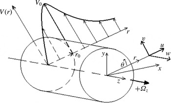
Velocity components
 $(u,v,w)$
in cylindrical
 $(r,{\it\theta},z)$
coordinates, and the mean velocity profile,
 $V(r)$
;
 $(x,y,z)$
are Cartesian coordinates. The core radius,
 $r_{0}$
, denotes the radius at
 $V_{0}$
, the maximum of
 $V$
. Note that core vorticity,
 $+{\it\Omega}z$
, is in
 $+z$
direction.

2 Methods
Instantaneous velocity
 $\boldsymbol{u}=(u,v,w)$
and vorticity
 ${\bf\omega}=({\it\omega}_{r},{\it\omega}_{{\it\theta}},{\it\omega}_{z})$
in cylindrical coordinates
 $(r,{\it\theta},z)$
are shown in figure 1.
 $(x,y,z)$
denote Cartesian coordinates. Mean quantities are averaged over
 ${\it\theta}$
and
 $z$
at each time and are denoted with uppercase letters, e.g. mean azimuthal velocity
 $(V)$
; primes denote fluctuation quantities, e.g. radial perturbation vorticity,
 ${\it\omega}_{r}^{\prime }$
, which go to zero as
 $r$
goes to infinity. Overbars, e.g.
 $\overline{u^{\prime }v^{\prime }}$
, denote the average over
 ${\it\theta}$
and
 $z$
of fluctuation quantities.
A fourth-order accurate pseudospectral method, based on the Rennich & Lele (Reference Rennich and Lele1997) algorithm and detailed in Pradeep & Hussain (Reference Pradeep and Hussain2004), is used to correctly simulate an isolated vortex column. Consider the intrinsic constraint of periodic flow domains requiring the velocity at the domain boundary parallel to the vortex axis to be zero – which is not appropriate for flows with non-zero circulation such as those containing a prominent vortex. Outside this vortex (i.e. where vorticity is zero), the velocity field is purely potential, and given by the Biot–Savart law. The Rennich & Lele (Reference Rennich and Lele1997) algorithm calculates the potential velocity field throughout the domain by matching the velocity field within the computational domain – consisting of vortical plus potential velocity – to the Biot–Savart velocity outside the vortical region, thus removing the artefact of the infinite array of image vortices inherent to the periodic boundary condition, and correctly produces a velocity field as if the boundary was at infinite distance. The domain is periodic in the axial (
 $z$
) direction and ‘unbounded’ in the radial (
 $r$
, or
 $x$
and
 $y$
) direction at vortex Reynolds number (
 $Re\equiv \text{circulation}\text{/}\text{viscosity}={\it\Gamma}_{\infty }/{\it\nu}$
, where
 ${\it\Gamma}_{\infty }$
is computed around a circular contour with infinite radius) ranging from 500 to 12 500. For stability, the Courant–Friedrichs–Lewy (CFL) number is maintained at 0.75 (Moin Reference Moin2001) via an adaptive time-step size.
The initial mean axial vorticity of the Oseen vortex is
 $$\begin{eqnarray}{\it\Omega}_{z}(r)={\it\Omega}_{0}\exp (-(r/r_{1})^{2}),\end{eqnarray}$$
where
 ${\it\Omega}_{0}\,(=2)$
is the peak mean axial vorticity, and
 $r_{1}=1$
is a parameter in the velocity profile:
 $$\begin{eqnarray}V(r)=\frac{{\it\Gamma}}{2{\rm\pi}r}(1-\text{e}^{-(r/r_{1})^{2}}),\end{eqnarray}$$
where
 ${\it\Gamma}$
is the vortex circulation at infinity. The turnover time,
 $T^{\prime }=2{\rm\pi}r_{0}/V_{0}$
(where
 $r_{0}=1.12r_{1}=1.12$
is the core radius, i.e. the radius of peak azimuthal velocity, and
 $V_{0}=0.63$
is the peak azimuthal velocity) is the time it takes a fluid particle in the core to circle the core once; one turnover corresponds to
 $T^{\prime }=11$
. Time is normalized by the turnover time as
 $T=t/T^{\prime }$
. Thus,
 $T=1$
denotes one actual turnover time.
We consider two cases, where the Oseen vortex is embedded in: case (1) fine-scale turbulence at
 $Re=12\,500$
; and case (2) a perturbation without turbulence. The turbulence in case 1 is initiated using a random fluctuation field having the Mansour & Wray (Reference Mansour and Wray1994) spectrum peaking at
 $k=16$
– the structures containing the largest energy at
 $k=16$
, i.e. a length scale of
 $0.35r_{0}$
. The fluctuation field has an initial amplitude,
 $\hat{u} /V_{0}=20\,\%$
(where
 $\hat{u} ^{2}(r)$
is the perturbation kinetic energy averaged over a cylindrical surface of radius
 $r$
,
 $(2{\rm\pi}z_{l})^{-1}\int (u^{\prime 2}+v^{\prime 2}+w^{\prime 2})\,\text{d}{\it\theta}\,\text{d}z$
and
 $z_{l}$
is the computational axial length), which would develop into homogeneous, isotropic turbulence if simulated alone. In order to apply the Rennich & Lele (Reference Rennich and Lele1997) algorithm, we start with randomly generated, divergence-free velocity fluctuations using the specified energy spectrum, and radially filter it so that the vorticity outside the patch, within the domain boundary, is zero. The large initial amplitude is chosen so that the fluctuations survive the initial dissipation and evolve later in time. The perturbation in case 2 is helical (azimuthal wavenumber
 $m=1$
) with an initial amplitude of
 $\hat{u} /V_{0}\approx 8\,\%$
. The computational domain and mesh sizes for the two cases are
 $x_{l}\times y_{l}\times z_{l}=10\sqrt{2}\times 10\sqrt{2}\times 14{\rm\pi}$
and
 $n_{x}\times n_{y}\times n_{z}=192\times 192\times 512$
, and
 $10\sqrt{2}\times 10\sqrt{2}\times 2{\rm\pi}/1.4$
and
 $384\times 384\times 128$
respectively. The smallest length scales in the domains are
 $h_{1}\,(=z_{l}/n_{z})=0.073$
for case 1, and
 $h_{2}\,(=z_{l}/n_{z})=0.012$
for case 2. The Kolmogorov length scales (at the time of peak dissipation) are
 ${\it\eta}_{1}=0.041$
and
 ${\it\eta}_{2}=0.046$
. In both cases, the Kolmogorov length scales are similar to/smaller than the smallest turbulence scales, indicating the two cases are well resolved. Note that, for case 2, the smallest grid spacing occurs in the axial direction, which should be well resolved at all times, as a cascade of axial scales does not occur. Additionally, for both cases, the enstrophy spectra at all times (not shown) maintain more than a decade falloff at high wavenumbers, indicating no aliasing issues.
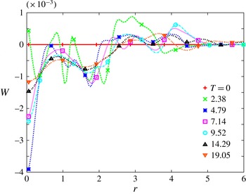
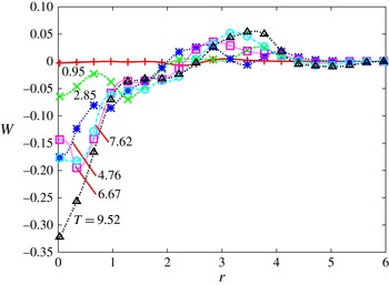
Profiles of mean axial velocity,
 $W$
, at seven times for vortex–turbulence interaction at
 $Re=12\,500$
; note that
 $W\,(T=0)=0$
.
 $W(r)$
here is rather weak, approximately 100 times smaller than the
 $W(r)$
generated for the helical perturbation (figure 6). Note that there are nine computational data points between adjacent symbols on each curve.

3 Case 1: ambient turbulence
To motivate our analysis of axial flow generation, consider a simulation of the Oseen vortex embedded in fine-scale turbulence at
 $Re=12\,500$
. The dynamics of vortex–turbulence interaction are briefly reviewed (detailed in PH10), culminating with evidence that the turbulent field generates flow parallel to the vortex axis.
The initial turbulence within the column decreases by dissipation due to the absence of straining, but the turbulence outside the column is wrapped around the column axis by the mean swirl, forming azimuthal vorticity filaments (see PH10). These filaments self-advect predominantly, though not purely, in the axial (
 $z$
) direction, and filaments of opposite circulations form vortex dipoles; filaments with the same circulation undergo pairing into a larger filament with their combined circulation. As the filaments evolve, they generate negative
 $u^{\prime }v^{\prime }$
Reynolds stress, causing perturbation energy growth (due to negative mean shear, PH06). Filament dipoles then viscously cross-annihilate, leading to energy decay and leaving only a few individual filaments, either unpaired or as the remnants of unequal strength filament dipoles, at late times.
Evolution of the profiles of mean axial flow,
 $W(r)$
(figure 2), shows development of non-negligible flow near the axis. Generation of mean axial flow (
 $W$
) indicates that the initially equal positive and negative perturbation azimuthal vorticities
 $({\it\omega}_{{\it\theta}}^{\prime })$
at each radius become unequal. The direction of the axial flow rapidly fluctuates at early times due to the reorganization (interaction and pairing of adjacent filaments) of the external turbulent field, hence their induced flows in the core (PH10). Between
 $T\approx 7$
and
 $T\approx 9$
, after the filaments have formed (PH10), there is a slight increase in the magnitude of
 $W_{max}$
, indicating potential (steady) generation of axial flow – explored later. After
 $T\approx 9,|W_{max}|$
and
 $W(r)$
profiles decay as the filaments outside the core viscously diffuse and cross-annihilate (PH10), which ends axial flow generation and results in viscous decay of
 $W(r)$
.
4 Axial flow generation
Motivated by the axial flow observed in case 1 (figure 2), the axial flow generating mechanism is first sought via the Reynolds-averaged Navier–Stokes (RANS) equation, which indicates vorticity filaments induce axial flow. A physical explanation is proposed, with details given in appendix A. Confirmation of the axial flow mechanism and the resulting change in the vortex dynamics are found via simulation of a helical perturbation.
Axial flow
 $(W)$
generation, shown in figure 2, is explained using the spatially averaged axial momentum equation:
 $$\begin{eqnarray}\frac{\partial W}{\partial t}+U\frac{\partial W}{\partial r}=-\frac{1}{r}\frac{\partial r\overline{u^{\prime }w^{\prime }}}{\partial r}+{\it\nu}\frac{1}{r}\frac{\partial }{\partial r}\left(r\frac{\partial W}{\partial r}\right),\end{eqnarray}$$
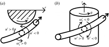
where the turbulent stress,
 $\overline{u^{\prime }w^{\prime }}$
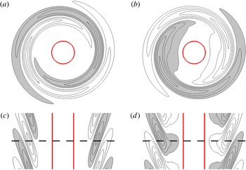
, associated with a vorticity filament (figure 3
a,b), drives axial flow; viscosity only causes diffusion and no generation of the axial flow.
Example filament generating
 $\overline{u^{\prime }w^{\prime }}>0$
due to (a)
 $u^{\prime }$
, associated with
 ${\it\omega}_{z}^{\prime }$
(in this case
 ${\it\omega}_{z}^{\prime }>0$
), and (b)
 $w^{\prime }$
, associated with
 ${\it\omega}_{r}^{\prime }$
(in this case
 ${\it\omega}_{r}^{\prime }<0$
). Note that
 ${\it\omega}_{r}^{\prime }$
and
 ${\it\omega}_{z}^{\prime }$
can have any combination of orientations (i.e.
 ${\it\omega}_{r}^{\prime }>0$
and
 ${\it\omega}_{z}^{\prime }>0$
or vice versa).

Tilting of radial perturbation vorticity
 $({\it\omega}_{r}^{\prime })$
into azimuthal perturbation vorticity
 $({\it\omega}_{{\it\theta}}^{\prime })$
without loss, i.e. mean straining of the vorticity field, linearly increases
 $u^{\prime }$
, thus also
 $\overline{u^{\prime }w^{\prime }}$
; by continuity,
 $w^{\prime }$
also increases linearly (PH06). The maximal growth rate possible for
 $\overline{u^{\prime }w^{\prime }}$
is quadratic in time. The sign of
 $\overline{u^{\prime }w^{\prime }}$
is determined by the circulation and initial orientation of the filament, thus the direction of axial flow is controlled by the initial condition of the filament. Axial flow
 $(W)$
has a range of growth rates, from (4.1), between zero and cubic in time depending on the relative phase between
 $u^{\prime }$
and
 $w^{\prime }$
, which determines
 $\overline{u^{\prime }w^{\prime }}$
. Based on this, at high
 $Re$
, even small perturbations will produce appreciable axial flow over long periods of time. For a short time frame (say, up to turnover times
 $T=10$
), if we assume that (i)
 $W$
grows quadratically in time (i.e.
 $W_{max}\approx T^{2}\overline{u^{\prime }w^{\prime }}_{max}$
), (ii)
 $q=V_{max}/W_{max}=100$
indicates appreciable axial flow, and (iii)
 $\overline{u^{\prime }w^{\prime }}_{max}$
can be up to
 $A^{2}V_{max}^{2}$
(where
 $A$
is a coefficient for the magnitude of
 $u^{\prime }$
and
 $w^{\prime }$
), then
 $W_{max}\sim T^{2}\overline{u^{\prime }w^{\prime }}_{max}\sim A^{2}T^{2}V_{max}^{2}\sim A^{2}(10^{2})(100^{2}W_{max})$
; hence, axial flow is generated by a single pair of filaments with a minimum intensity of
 $A=O(10^{-8})$
. Thus, extremely small perturbations can generate appreciable axial flow. Clearly, axial flow in vortex–turbulence interaction (figure 2) can vary as multiple filament pairs can superimpose to produce any amplitude axial flow, even a weak flow. Analysis of the self-induced motion of a pair of idealized, isolated vortex filaments shows how circulation and orientation of the filament are critical to the generation of
 $W$
(see appendix A).
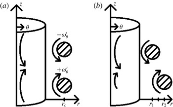
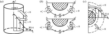
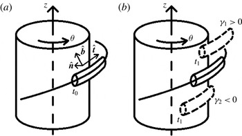
Because of the strong azimuthal wrapping, axial inclination and radial extent of the vortex filament in figure 3, the self-advection normal to the plane of the filament is predominantly axial, with a radial component (further detailed in appendix A, see discussion of figure 25). A pair of vorticity filaments with opposite circulations radially separate (figure 4
a), resulting in the velocities along the column axis induced by the filament pair becoming unequal and generating axial flow (
 $W$
, figure 4
b). This can be seen through application of the local induction approximation to a non-axisymmetric vorticity filament, and then treating the induced axial velocity of each filament as that of a vortex ring – hence, the induced velocity is inversely proportional to the filament’s radial distance. Note that treating the filament as a vortex ring overestimates the axial flow, as
 $W$
is reduced by non-zero
 ${\it\omega}_{r}$
and
 ${\it\omega}_{z}$
, and initial
 ${\it\omega}_{{\it\theta}}$
.
(a) Cross-sectional sketch of two oppositely oriented filaments with
 $+{\it\omega}_{{\it\theta}}^{\prime }$
and
 $-{\it\omega}_{{\it\theta}}^{\prime }$
at the same radius,
 $r_{c}$
, and their induced flows at the axis. (b) Filaments’ positions at a later time, resulting in a net axial flow (the difference between the two arrows).

5 Case 2: vortex–perturbation interaction
To provide further evidence that the mechanism described above is indeed the cause of axial flow generation, we now analyse the Oseen vortex with a perturbation containing only the key features of the mechanism (i.e. advection of vorticity filaments), and none of the complications (e.g. pairing, cross-annihilation etc.) associated with starting from a random turbulent field. This simplified case, studied over a range of
 $Re$
(500–10 000), provides a model for what would be expected at higher
 $Re$
values, beyond current computer capability.
We use a helical (azimuthal wavenumber
 $m=1$
, axial wavenumber,
 $k=1.4$
) optimal perturbation (largest energy growth in the linear case; found using the technique discussed in PH06) for
 $Re=5000$
, shown in figure 5. Optimal perturbations at increasing
 $Re$
consist of ever-tightening spiral threads (HPS); e.g. the
 $Re=10\,000$
optimal perturbation consisting of packed threads of adjacent, oppositely signed vorticity would rapidly cross-annihilate at low
 $Re$
and hence would not produce noticeable axial flow. Thus a moderate
 $Re$
optimal perturbation is studied over the
 $Re$
range of 500–10 000. Note that axisymmetric threads produce no axial flow (see appendix A), making the helical
 $(m=1)$
perturbation the lowest azimuthal wavenumber that relates to the dynamics of interest. Additionally, the helical optimal perturbation is the dominant mode during vortex–turbulence interaction for the
 $Re$
range studied, and we expect this to remain so in yet inaccessible, very high
 $Re$
cases (computationally unachievable). First, we focus on axial flow generation over the
 $Re$
range of 500–10 000. Then, evolution of the transient growth (helical) perturbation at
 $Re=10\,000$
is examined to explain the late-time renewed energy growth and its connection to axial flow.
Axial (
 $x$
–
 $y$
) plane contours of (a)
 ${\it\omega}_{r}^{\prime }$
and (b)
 ${\it\omega}_{{\it\theta}}^{\prime }$
, and meridional (
 $z$
–
 $x$
) plane contours of (c)
 ${\it\omega}_{r}^{\prime }$
and (d)
 ${\it\omega}_{{\it\theta}}^{\prime }$
showing the initial helical transient growth optimal perturbation; (a) and (b) are the cross-sectional views of (c) and (d) at the dashed line. Contour levels are
 ${\it\delta}{\it\omega}_{r}^{\prime }=0.2$
and
 ${\it\delta}{\it\omega}_{{\it\theta}}^{\prime }=0.02$
; the thick (red) line shows the vortex core at
 $|{\it\omega}|=1$
. Shaded regions indicate negative values.

Profiles of
 $W$
at six times for the helical perturbation at
 $Re=10\,000$
; note that initially
 $W=0$
. Between
 $T=4.76$
and 7.62, there is a decrease in
 $W$
at the axis, due to distortion of the axis (discussed later, in connection with figure 10). Note that there are nine data points between adjacent symbols on each curve.

Note that generation of axial flow depends on the circulation and spatial orientation of the filaments (see appendix A). Higher azimuthal wavenumbers (i.e.
 $|m|>1$
) mean a greater number of filament pairs undergoing radial advection, which would produce greater axial flow (as all the filament pairs would have the same orientation and undergo the same evolution, the effects being additive). A greater number of filaments would viscously cross-annihilate faster, limiting the overall axial flow production. Axial periodicity of the helical perturbation computationally means it is infinitely long, and the induced axial velocity is that for an infinitely long filament (Hardin Reference Hardin1982), but not that for a finite length filament (as occurs in vortex–turbulence interaction, PH10). However, the axial flow mechanism is due to local dynamics, and does not involve axial periodicity.
Profiles of
 $W$
(figure 6) at
 $Re=10\,000$
show development of significant axial flow within the vortex core. Axial flow opposite to that on the axis develops due to the invariant zero meridional circulation (since
 $W=0$
initially). Deflection of the vortex axis causes the peak axial velocity magnitude,
 $|W_{max}|$
, to occur off the axis, e.g. at
 $T=2.85$
and
 $T=6.67$
(figure 6) – due to helical deflection of the vortex axis (discussed later in connection with figure 10). Note that the profiles near the axis are similar to those for the Batchelor vortex, i.e. Gaussian-like; thus the vortex dynamics of the familiar Batchelor vortex apply here (discussed below). Zero axial momentum (integral of
 $W$
profile) is conserved, with the volume-integrated axial momentum (non-dimensionalized as
 $\int 2{\rm\pi}z_{l}Wr\,\text{d}r/(A{\it\Gamma}_{\infty })$
, where
 $A$
is the computational domain cross-section perpendicular to the vortex axis) peaking at
 $3.7\times 10^{-4}$
.
The radii where
 $W$
first equals zero for the turbulent case (
 $r\approx 2.5$
at
 $T=19.05$
, figure 2) and also the helical perturbation case (
 $r\approx 2.5$
at
 $T=9.52$
, figure 6) are approximately equal. HPS observed that the transiently growing optimal perturbation contributes the most to the late-time energy in vortex–turbulence interaction, indicating the axial flow in the turbulence case is generated by the same mechanism as for the helical perturbation. Note that, for the two cases, the axial lengths of the computational domains are infinite via periodicity; thus, axial length plays no role in axial flow generation – either case emphasizing the sole role of local dynamics in axial flow generation. The vortex column becomes unstable for large axial velocities (Lessen et al.
Reference Lessen, Singh and Paillet1974) – therefore it is of interest to examine the evolution of the peak axial velocity.
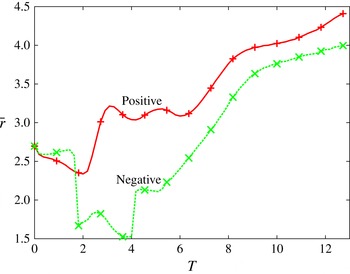
Evolution of the centroid
 $(\bar{r})$
of positive
 ${\it\omega}_{{\it\theta}}$
(red
 $+$
) and negative
 ${\it\omega}_{{\it\theta}}$
(green
 $\times$
) for the filaments outside the core at
 $Re=10\,000$
in the (
 $r$
–
 $z$
) meridional plane.

To capture the radial movement of the vorticity filaments, take the evolution of their centroids (calculated using
 ${\it\omega}_{{\it\theta}}$
above 95 % of the maximum of each for
 $r>1.5$
; figure 7). The high threshold for the vorticity values is used to identify and track the initial filament pair, independent of additional filaments that develop later. The initial relative radial movement between the two filaments depends on their initial configuration (as discussed in appendix A). The two form a dipole by
 $T\sim 6$
, beyond which it moves with nearly constant separation between the filaments. The inner filament dominates the generation of axial flow. The initial radial separation of the filaments confirms the proposed mechanism: axial flow originates from relative radial advection of filaments.
As a brief aside, vortex–turbulence interaction evolves to be eventually dominated by the helical transient growth optimal perturbation (HPS) – hence the directions of axial flow generated for turbulence (case 1) and the helical perturbation (case 2) are the same (compare figures 2 and 6). As the direction of axial flow is controlled by the self-advection of the filaments comprising the helical perturbation (see appendix A), negative axial flow naturally arises in vortex–turbulence interaction. At early times in vortex–turbulence interaction, other filaments can undergo self-advection and generate axial flow in either direction. This reduces the magnitude of the axial flow and causes fluctuations for the turbulent case (figure 2). Note that the turbulence is more than double the initial intensity of the transient growth mode, but produces almost two orders of magnitude weaker axial flow. Additionally, the filaments formed from the turbulent initial condition in case 1 have much smaller individual circulation (estimated, as in HPS), and thus generate smaller axial flow than in case 2 – a single pair of filaments with significant circulation. Based on the natural emergence of the helical transient growth optimal, it seems unlikely that positive axial flow will be generated in vortex–turbulence interaction, though a tailored perturbation could cause it.
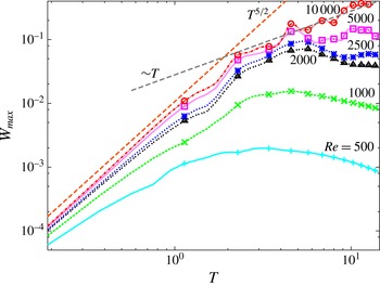
Growth of
 $|W_{max}|$
for the helical perturbation, showing an early time trend of
 $T^{5/2}$
until
 $T\approx 2$
(for high
 $Re$
), which is followed by slower growth.

The evolution of
 $|W_{max}|$
for a range of
 $Re$
values shows significant growth over the first two turnover times (figure 8). With increasing
 $Re$
, decreasing viscous cross-annihilation of the filaments which drive axial flow generation results in greater
 $|W_{max}|$
(compare
 $Re=500$
and 10 000, figure 8). The calculated growth rate at early times,
 $W\sim T^{5/2}$
, falls within the range of growth rates discussed in § 4, with the reduction caused by the neglected role of a filament’s
 ${\it\omega}_{r}^{\prime }$
and
 ${\it\omega}_{z}^{\prime }$
slowing the self-induced radial advection. At later times, dipole formation causes mutual advection of the two filaments radially outwards, which dominates the radial part of either filament’s self-advection (figure 7); additionally, dipole formation increases viscous cross-annihilation of the two filaments, reducing the filaments’ circulations. Together, these effects slow
 $W$
growth. Note that there are fluctuations in the evolution of
 $|W_{max}|$
in figure 8, discussed next.
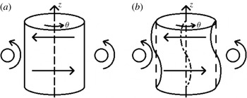
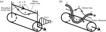
(a) An initially rectilinear vortex column is perturbed with a helical
 $(m=1)$
perturbation. (b) The perturbation’s induced velocity displaces the axis, causing the vortex to become helical.

(a) Evolution of the vorticity magnitude centroid relative to the initial position
 $(\bar{r})$
due to the helical perturbation, denoting the centre of the vortex, at
 $Re=10\,000$
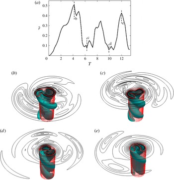
; b, c, d, e respectively denote the times of realizations given in (b), (c), (d), (e). Core distortion, shown by the
 $|{\it\omega}|=1$
surface, in relation to the original vortex core of
 $r=1.12$
(transparent cylinder) and vorticity magnitude isocontours (red indicating the core at
 $|{\it\omega}|=1$
) at (b)
 $T=4.2$
, (c)
 $T=6.2$
, (d)
 $T=10$
and (e)
 $T=12$
.

Fluctuations in
 $|W_{max}|$
at high
 $Re$
(figure 8) are caused by displacement of the vortex axis away from the coordinate axis due to the helical perturbation (sketched in figure 9). The displacement of the vortex axis from the
 $z$
-axis at
 $Re=10\,000$
is measured using
 $\bar{r}$
(figure 10
a), which is the axial average of the displacement of the vorticity magnitude centroid calculated at each
 $z$
(using vorticity above 75 % of the peak vorticity).
 $\bar{r}$
represents interesting geometrical effects of vortex displacement; for this, we will address flow along the vortex axis and its inclination with respect to the initial, undisplaced axis (denoted ‘axis’ here). Variations in
 $|W_{max}|$
(figure 8) – which correspond to those of
 $\bar{r}$
(figure 10
a) – can be due to two effects: (i) the displacement introduces inherent large variation of
 $|W|$
on the ‘axis’, and (ii) the distortion introduces an inclination of
 $|W_{max}|$
to the ‘axis’, seen in figure 10(b–e) – vorticity magnitude surfaces and their top end isocontours at four times compared to the original cylindrical core.
The helical filaments repeatedly displace the core radially (as in figure 9), as the filaments and core vorticity fluctuations rotate at slightly different rates. PH06 found resonance between the filaments’ and core fluctuations’ rotation rates causing growth; self-advection of the filaments modifies their rotation rates. The displacement by the filaments leads to the large
 $\bar{r}$
at
 $T=4.2$
(figure 10
b) with the core contour outside the initial core radius (the meshed column), with a distinct two-lobe structure (i.e.
 $|m|=2$
) due to the interaction of the filaments with the core fluctuations. A similar increase in the azimuthal as well as axial wavenumbers is discussed in § 6. Over time, the filaments rotate relative to the core and decrease the core displacement (figure 10
c). The third peak in
 $\bar{r}$
(
 $T=12$
) results from the combination of mean strain at the core edge and the displacement of the core due to the external filaments (figure 10
e). Interestingly, the core distortion at
 $T=12$
means the vortex is ‘hollow’, with the ‘axis’ no longer within the core contour – expected for a low-
 $q$
Batchelor vortex. Decreasing viscous cross-annihilation with increasing
 $Re$
generates greater oscillations of
 $\bar{r},|W_{max}|$
and
 $q$
, as well as greater flow along the vortex axis – potentially leading to vortex instability.
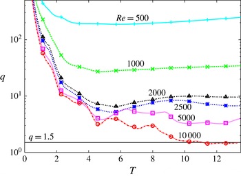
Evolution of
 $q=|V_{max}/W_{max}|$
for the helical perturbation at six values of
 $Re$
(500, 1000, 2000, 2500, 5000, 10 000), with
 $q=1.5$
marked by the horizontal line. At
 $T=11,q<1.5$
, suggesting that the vortex becomes unstable.

Starting with infinite value at
 $T=0$
,
 $q$
quickly drops (figure 11) because of rapid growth of
 $|W_{max}|$
(figure 8) for 2–4 turnover times, before levelling off as
 $W$
generation slows and ends (discussed above); thence both
 $V_{max}$
and
 $W_{max}$
viscously decay at late times. At
 $Re=10\,000$
, evolution of
 $q$
(figure 11) has fluctuations due to displacement of the core, similar to fluctuations in
 $|W_{max}|$
(figure 8). As
 $V_{max}$
generally decreases due to viscous diffusion, while
 $|W_{max}|$
increases due to the radial advection of the filaments (discussed above),
 $q=V_{max}/W_{max}$
decreases, thus leading to instability via the
 $q$
criterion.
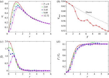
(a)
 $V$
profiles at five times, (b) evolution of
 $V_{max}$
, (c)
 ${\it\Omega}_{z}$
profiles at five times, and (d)
 ${\it\Gamma}$
profiles at five times for the helical perturbation for
 $Re=10\,000$
. Also shown in (b) is the theoretical viscous decay of
 $V_{max}$
for the laminar, Oseen vortex.

Let us discuss how
 $V_{max}$
and
 $V(r)$
evolve and affect
 $q$
evolution. Profiles of
 $V$
(figure 12
a) remain approximately self-similar as in viscous decay, especially outside the vortex core (
 $r>1$
); changes near the axis are related to the previously discussed displacement of the axis. The vortical
 $({\it\Omega}_{z})$
region extends to
 $r\approx 2$
(figure 12
c), outside which the profiles are essentially unchanged. The small changes in
 $V(r)$
at larger radius (near
 $r=3.5$
at
 $T=2.85$
, figure 12
a) are due to radial transport of azimuthal momentum, resulting in circulation overshoots (figure 12
d; with negative
 ${\it\Omega}_{z}$
corresponding to decreasing circulation) with negligible effect on the vorticity dynamics (Hussain & Stout Reference Hussain and Stout2013). Within the core,
 $V(r)$
changes beyond natural viscous diffusion are caused by deflection of the vortex axis, similar to those in
 $W$
(discussed above). Displacement of the core causes non-monotonic variation of
 $V_{max}$
(compare fluctuations in figure 10
a to those in figure 12
b); after the initial displacement decreases, the persisting helical distortion of the core (figure 10
b–e) means the azimuthal swirl around the core is inclined relative to the azimuthal direction, which reduces
 $V_{max}$
, similar to the effect of inclination on
 $|W_{max}|$
– discussed previously. Note that the large decrease in
 ${\it\Omega}_{z}$
at the axis (figure 12
c) is due to the helical distortion of the vortex column (previously discussed); the dynamics within the core is discussed in § 6. It is interesting to note that, after the initial rapid decrease, the decay rate of
 $V_{max}$
seems comparable to that of the laminar Oseen vortex (shown for comparison in figure 12
b).
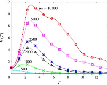
Evolution of the volume-averaged turbulent kinetic energy for the helical perturbation at six
 $Re$
values. Note that at
 $T\approx 6$
and
 $T\approx 11$
, for
 $Re=10\,000$
, the energy decay slows, indicating renewed energy production, possibly due to axial flow.

6 Late-time vortex dynamics
Based on the observed generation of axial flow, which reaches the instability limit of
 $q=1.5$
, the evolution of the helical perturbation is examined for the contribution of axial flow to the vorticity dynamics. First, the perturbation energy and axial flow evolutions are used to identify periods when axial flow may be important. As our previous study suggested a parent–offspring hairpin mechanism may drive renewed energy production (HPS), the vorticity dynamics for both the hairpin mechanism and vorticity generation due to axial flow are detailed next. Finally, the vorticity field during the periods of interest are examined and discussed for their relation to the hairpin and axial flow mechanisms.
Examining the volume-averaged perturbation energy,
 $E(T)=0.5\mathscr{V}^{-1}\int (u^{\prime 2}+v^{\prime 2}+w^{\prime 2})\,\text{d}\mathscr{V}$
, where
 $\mathscr{V}$
is the computational volume (figure 13), for
 $Re=10\,000$
, there are two notable periods where energy decay is significantly slowed due to renewed energy production after the energy peak – one at
 $T\sim 6$
and the second at
 $T\sim 11$
. The second period of renewed energy production occurs at the same time as
 $q$
decreases below the critical value of 1.5 (figure 11, marked by the horizontal line), indicating axial flow may result in instability. Note that the peak
 $E$
occurs at
 $T\sim 2.3$
at all values of
 $Re$
, presumably because the growth mechanism is inherently inviscid (PH06). However, HPS proposed a parent–offspring hairpin mechanism for renewed energy growth independent of axial flow. To determine the source of the growth, the hairpin mechanism discussed in HPS and vorticity generation due to axial flow are both discussed next, and then vorticity contours are used to determine the dominant mechanism for late-time renewed growth.
Postulated parent–offspring hairpin vortex mechanism from HPS.

The HPS parent–offspring hairpin vortex mechanism occurs when an initially radially displaced vortex line (figure 14 a) is wrapped azimuthally by the mean strain, generating the parent hairpin filament, which then perturbs other vortex lines radially (figure 14 b). The newly perturbed vortex lines intensify due to mean straining to form an offspring hairpin, while also generating perturbation energy. Note that the hairpin mechanism does not depend on the parent filament to be shaped like a hairpin; two azimuthally oriented vorticity filaments in a dipole tilt vortex lines radially like in figure 14, and move radially outward as a dipole, as seen later in figure 19.
To understand vorticity generation and instability (i.e. energy growth) due to axial flow, consider the linearized perturbation vorticity equations for a Batchelor vortex,
 $$\begin{eqnarray}\displaystyle & \displaystyle \frac{\text{D}{\it\omega}_{r}^{\prime }}{\text{D}t}=\frac{{\it\Omega}_{{\it\theta}}}{r}\frac{\partial u^{\prime }}{\partial {\it\theta}}+{\it\Omega}_{z}\frac{\partial u^{\prime }}{\partial z}, & \displaystyle\end{eqnarray}$$
 $$\begin{eqnarray}\displaystyle & \displaystyle \frac{\text{D}{\it\omega}_{{\it\theta}}^{\prime }}{\text{D}t}=\frac{{\it\Omega}_{{\it\theta}}}{r}\frac{\partial v^{\prime }}{\partial {\it\theta}}+{\it\Omega}_{z}\frac{\partial v^{\prime }}{\partial z}+S{\it\omega}_{r}^{\prime }+\frac{u^{\prime }{\it\Omega}_{{\it\theta}}}{r}, & \displaystyle\end{eqnarray}$$
 $$\begin{eqnarray}\displaystyle & \displaystyle \frac{\text{D}{\it\omega}_{z}^{\prime }}{\text{D}t}=\frac{{\it\Omega}_{{\it\theta}}}{r}\frac{\partial w^{\prime }}{\partial {\it\theta}}+{\it\Omega}_{z}\frac{\partial w^{\prime }}{\partial z}+{\it\omega}_{r}^{\prime }\frac{\partial W}{\partial r}, & \displaystyle\end{eqnarray}$$
where
 $S=r\partial (V/r)/\partial r$
is the mean strain rate due to
 $V$
,
 $\text{D}(\cdot )/\text{D}t=\partial (\cdot )/\partial t+U\partial (\cdot )/\partial r+(V/r)\partial (\cdot )/\partial {\it\theta}+W\partial (\cdot )/\partial z$
, and
 ${\it\Omega}_{{\it\theta}}=-\partial W/\partial r$
.
Axial flow,
 $W(r)$
, causes a filament initially composed of radial perturbation vorticity
 $({\it\omega}_{r}^{\prime })$
to tilt into axial perturbation vorticity
 $({\it\omega}_{z}^{\prime })$
by the mean shear
 $\partial W/\partial r$
(via (6.3); figure 15
a). Mean azimuthal vorticity contributes to vorticity generation in two ways:
 $({\it\Omega}_{{\it\theta}}/r)\partial \boldsymbol{u}^{\prime }/\partial {\it\theta}$
in (6.1)–(6.3), which corresponds to tilting or stretching of the mean azimuthal vorticity (circles concentric with the vortex core) into the three directions
 $(r,{\it\theta},z)$
; and
 $(u^{\prime }{\it\Omega}_{{\it\theta}})/r$
in (6.2), which is radial transport of
 ${\it\Omega}_{{\it\theta}}$
by the radial perturbation velocity. Tilting of
 ${\it\Omega}_{{\it\theta}}$
by
 $\partial u^{\prime }/\partial {\it\theta}$
, associated with non-axisymmetric
 ${\it\omega}_{z}^{\prime }$
, generates
 ${\it\omega}_{r}^{\prime }$
in (6.1) (figure 15
b). Thus, initial
 ${\it\omega}_{r}^{\prime }$
generates
 ${\it\omega}_{z}^{\prime }$
due to tilting by
 $\partial W/\partial r$
, which in turn increases
 ${\it\omega}_{r}^{\prime }$
via tilting of the mean azimuthal vortex lines by
 $({\it\Omega}_{{\it\theta}}/r)\partial u^{\prime }/\partial {\it\theta}$
, thus continuously increasing both
 ${\it\omega}_{r}^{\prime }$
and
 ${\it\omega}_{z}^{\prime }$
. Concurrent with this intensification is tilting of
 ${\it\omega}_{r}^{\prime }$
into
 ${\it\omega}_{{\it\theta}}^{\prime }$
by
 $S$
(figure 15
c), resulting in simultaneous amplification of all three perturbation vorticity components (see Heaton & Peake Reference Heaton and Peake2007) and perturbation energy growth; hence this chain of vorticity generation is the physical mechanism of instability due to axial flow. These fairly straightforward descriptions of mechanisms are given to enable later discussion.
Vorticity generation due to (a) axial flow tilting perturbation radial vorticity
 $({\it\omega}_{r}^{\prime })$
, (b) perturbation axial vorticity
 $({\it\omega}_{z}^{\prime })$
tilting mean azimuthal vorticity
 $({\it\Omega}_{{\it\theta}})$
, and (c) mean strain tilting
 $({\it\omega}_{r}^{\prime })$
into perturbation azimuthal vorticity
 $({\it\omega}_{{\it\theta}}^{\prime })$
.

Note that the filaments encircling the vortex column are responsible for transport of energy out of the vortex core via the
 $\overline{u^{\prime }v^{\prime }}$
Reynolds stress. The dispersion of filaments along the axis as waves due to mean axial vorticity causes the Reynolds stress to advect and oscillate in both space and time, and produces no net transport. This limits the energy transport out of the core (discussed by Melander & Hussain (Reference Melander and Hussain1994) for the Oseen vortex, and by Jacquin & Pantano (Reference Jacquin and Pantano2002) for the Batchelor vortex). Only for low values of
 $q$
(
 $q<0.7$
, Jacquin & Pantano Reference Jacquin and Pantano2002) does the perturbation grow large enough to transport significant energy out of the core. For the helical perturbation, filaments occurring near the core grow due to axial flow, which produces Reynolds stress and energy transport, potentially overcoming the limiting effects of axial vorticity. This effect will be accentuated at higher Reynolds numbers, as reduced viscous effects would produce larger growth, and potentially lead to vortex breakup.
Exponential growth of vorticity is shown by approximating (6.1)–(6.3). First, assume
 ${\it\Omega}_{z}$
, which limits vorticity generation via core dynamics (Melander & Hussain Reference Melander and Hussain1994), is negligible compared to
 ${\it\Omega}_{{\it\theta}}$
. Next, approximate
 $(1/r)\partial u^{\prime }/\partial {\it\theta}\approx m{\it\omega}_{z}^{\prime }$
and
 $(1/r)\partial w^{\prime }/\partial {\it\theta}-{\it\omega}_{r}^{\prime }\approx m{\it\omega}_{r}^{\prime }$
, which captures the role of azimuthal variation on perturbation growth. Equation (6.1) then reduces to
 $\text{D}{\it\omega}_{r}^{\prime }/\text{D}t=-m{\it\Omega}_{{\it\theta}}{\it\omega}_{z}^{\prime }$
, and, using
 $\partial W/\partial r=-{\it\Omega}_{{\it\theta}}$
, (6.3) reduces to
 $\text{D}{\it\omega}_{z}^{\prime }/\text{D}t=-m{\it\Omega}_{{\it\theta}}{\it\omega}_{r}^{\prime }$
. Note that
 ${\it\omega}_{{\it\theta}}^{\prime }$
has no effect on
 ${\it\omega}_{r}^{\prime }$
or
 ${\it\omega}_{z}^{\prime }$
generation due to these approximations, as it primarily effects
 ${\it\omega}_{r}^{\prime }$
through core dynamics; growth of
 ${\it\omega}_{{\it\theta}}^{\prime }$
directly depends on growth of
 ${\it\omega}_{r}^{\prime }$
and
 ${\it\omega}_{z}^{\prime }$
. Solving
 $\text{D}{\it\omega}_{r}^{\prime }/\text{D}t=-m{\it\Omega}_{{\it\theta}}{\it\omega}_{z}^{\prime }$
and
 $\text{D}{\it\omega}_{z}^{\prime }/\text{D}t=-m{\it\Omega}_{{\it\theta}}{\it\omega}_{r}^{\prime }$
simultaneously gives
 ${\it\omega}_{r}^{\prime }={\it\omega}_{z}^{\prime }=C\,\exp (-m{\it\Omega}_{{\it\theta}}t)$
, where
 $C$
is a constant; thus there is instability either when
 ${\it\Omega}_{{\it\theta}}<0$
(the case here) or when
 $m<0$
. As vorticity generation is primarily by tilting, the perturbation length scales remain approximately constant and vorticity generation means energy production. Additionally, if
 ${\it\Omega}_{z}$
is included in the analysis, vorticity generation occurs when
 ${\it\Omega}_{{\it\theta}}>{\it\Omega}_{z}$
. For a perturbation near
 $r=1$
, where
 ${\it\Omega}_{{\it\theta}}$
peaks, this ratio becomes
 $2W_{max}\text{e}^{-1}>2V_{max}\text{e}^{-1}$
or
 $V_{max}/W_{max}=q<1$
– roughly approximating the inviscid instability limit of
 $q=1.5$
.
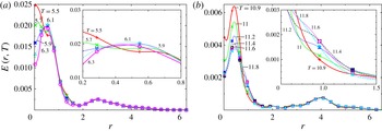
Profiles of
 $E(r,T)$
at six times during the (a) first period and (b) second period (from
 $T\approx 5.5$
to
 $T\approx 6.5$
and
 $T\approx 11$
to
 $T\approx 12$
, respectively) of regenerative growth in figure 13, for
 $Re=10\,000$
. Inset shows the region of
 $E(r,T)$
growth.

To identify the spatial regions of interest for regenerative growth, the turbulent kinetic energy profiles,
 $E(r,T)\,(=0.5(2{\rm\pi}z_{l})^{-1}\int (u^{\prime 2}+v^{\prime 2}+w^{\prime 2})r\,\text{d}{\it\theta}\,\text{d}z)$
, during the two periods of slowed energy decay (
 $T\approx 5.5{-}6.3$
and
 $T\approx 11{-}12$
for
 $Re=10\,000$
in figure 11) are shown (figure 16). For both times, the largest energy peak within the core occurs at
 $r=0.5$
(except at
 $T=5.5$
in figure 16
a), which is most likely due to the artefact of displacement of the vortex axis (confirmed by
 $\bar{r}$
in figure 10). The peak decreases as the displacement decays (figure 10
a); additionally core energy decreases, as the filaments encircling the core no longer generate core fluctuations (discussed in HPS) and the core fluctuations viscously decay. Note that the first growth period corresponds to the small peak near
 $T=5.5$
in figure 10(a). The vorticity filaments generated by intensification of the initial perturbation (in figure 5) are small energy peaks outside the core at
 $r\approx 3$
(figure 16
a) and at
 $r\approx 4$
(figure 16
b). Separate from these filaments, there are regions where the perturbation energy increases, specifically near
 $r\approx 0.5$
at
 $T\sim 6$
(inset, figure 16
a) and near
 $r\approx 1$
at
 $T\sim 11$
(inset, figure 16
b). By comparing the regions of energy growth and the evolution of the vorticity field, the role of the hairpin mechanism and vorticity generation due to axial flow can be evaluated for their effects on vortex dynamics. Note that in a viscous flow, vorticity tracking is not meaningful, as vortex lines are not material lines, and the dominant azimuthal vorticity is adequate to identify the filaments (i.e. more complex identification methods such as
 $Q$
or
 ${\it\lambda}_{2}$
, detailed by Jeong & Hussain (Reference Jeong and Hussain1995), will not help).
The evolution of the perturbation up to the first period (
 $T\approx 5.5$
) of renewed growth is briefly discussed (discussed in further detail by HPS) so that the subsequent evolution during the period of renewed energy growth can be interpreted. The initial perturbation radial vorticity (figure 5) is wrapped azimuthally (figure 15
c), generating two azimuthally oriented filaments, which produce energy growth (the early increase in figure 13). Axial flow is generated as the filaments self-advect and radial separate, seen in figure 7 and also in the vorticity contours discussed next. Limiting energy growth is viscosity and the tilting of mean axial vorticity (weak outside the core), which disperses the perturbation as waves – termed ‘core dynamics’ (Melander & Hussain Reference Melander and Hussain1994). Additionally, the filaments, located outside the core, generate fluctuations within the core by tilting vorticity (PH06). The filaments self-advect in the axial direction to form a dipole, which then radially advects outwards – also limiting energy growth as the filaments move to regions of reduced strain. The dipole’s induced motion tilts axial vortex lines radially beneath it, which forms additional filaments (i.e. the hairpin mechanism). Independent of the offspring filaments, several small vorticity patches (both in size and magnitude) occur due to tilting of mean axial vorticity outside the core; these have negligible effect on the flow evolution. The filament dipole, the potential offspring filaments and core fluctuations are the features present at the onset of the energy production which counters the viscous decay of the perturbation at
 $T\approx 5.5$
.
Meridional (
 $z$
–
 $x$
) plane contours of
 ${\it\omega}_{{\it\theta}}$
(a–c) and
 ${\it\omega}_{r}$
(d–f) before and during the first period of reduced energy decay (
 $T\sim 5.9$
in figure 16). Shaded regions denote negative vorticity; levels are plotted at
 $|{\it\omega}_{{\it\theta}}|=[{\it\omega}_{min},{\it\delta}{\it\omega}]=[0.1,0.1]$
,
 $|{\it\omega}_{r}|=[0.1,0.1]$
and
 $|{\it\omega}_{r}|=[{\it\omega}_{min},{\it\delta}{\it\omega},{\it\omega}_{max}]=[0.02,0.02,0.1]$
to capture the details. The core is shown as
 $|{\it\omega}|=0.5$
(red); note that distortion of the column causes a hollow area in the core. Additionally, a filament outside the core is seen from
 $T=5.9$
onwards: (a,d)
 $T=5.1$
, (b,e)
 $T=5.9$
, (c,f)
 $T=6.7$
.

Illustrating the vorticity dynamics during the periods of renewed growth (
 $T\approx 5.5{-}6.3$
and
 $T\approx 11{-}12$
) are contours of
 ${\it\omega}_{{\it\theta}}$
in a meridional (
 $z$
–
 $x$
) plane (figures 17
a–c and 19
a–c, respectively), and contours of
 ${\it\omega}_{r}$
in a meridional plane (figures 17
d–f and 19
d–f, respectively); for the second period of renewed growth, filaments encircling the core are shown using
 ${\it\omega}_{r}$
and
 ${\it\omega}_{{\it\theta}}$
isosurfaces in a quadrant. Note that the axial flow is downward. The helical distortion of the vorticity field during the second period is shown by the vorticity surfaces in figure 20. Contours of
 ${\it\omega}_{{\it\theta}}$
and
 ${\it\omega}_{r}$
in an axial (
 $x$
–
 $y$
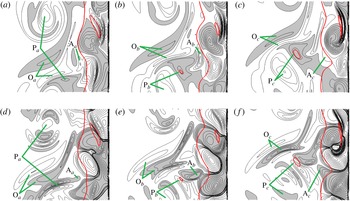
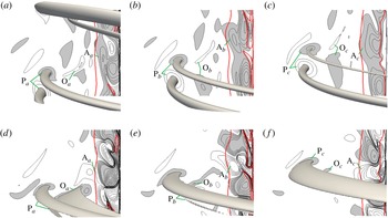
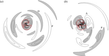
) plane (figure 21) illustrate the core dynamics and the filaments, discussed in conjunction with the vorticity surfaces in figure 20. Features of interest are marked P (parent), O (offspring) and A (axial) in figures 17, 19 and 21. First, the dynamics in the core are discussed, then the filaments encircling the core which act as parent filaments are examined and, finally, the effect of axial flow on vorticity generation is addressed.
The most noticeable features of the vortex core (within the thick red contour, figures 17 and 19) are the ‘cells’ of radial vorticity (figures 17
d–f and 19
d–f) and azimuthal vorticity (figures 17
a–c and 19
a–c) – generated by tilting of core vortex lines by filaments into the radial direction, which then are coiled/uncoiled by differential core rotation (i.e. core dynamics). Note that both the azimuthal vorticity
 $({\it\omega}_{{\it\theta}})$
‘cells’ have the same sign, thus each
 ${\it\omega}_{{\it\theta}}$
cell produces two
 ${\it\omega}_{r}$
cells due to the presence of the neighbouring
 ${\it\omega}_{{\it\theta}}$
cells, doubling the axial wavenumber of the core fluctuations. Strong distortion of the vortex column can lead to the core contour appearing hollow, like in figure 17, a result of using vorticity magnitude to capture the core. For the later time period of production, the vortex core in an axial (
 $x$
–
 $y$
) plane (thick red contour in figure 21) is hollow, as one of the positive
 ${\it\omega}_{{\it\theta}}$
cells (like one of the four cells in figure 21
b) has moved to the centre due to the distortion of the core. This advection of vorticity towards the axis is traced to the self-induced radial advection of the filament, wherein one of the external filaments moves closer to the core, which generates stronger core fluctuations.
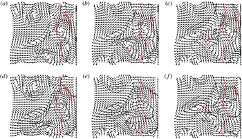
Velocity direction vectors in the meridional (
 $z$
–
 $x$
) plane with (grey) contours of
 $|{\it\omega}_{{\it\theta}}|=0.2$
(a–c) and
 $|{\it\omega}_{r}|=0.04$
(d–f) before and during the first period of reduced energy decay (
 $T\sim 5.9$
in figure 16). The core is indicated by
 $|{\it\omega}|=0.5$
(red): (a,d)
 $T=5.1$
, (b,e)
 $T=5.9$
, (c,f)
 $T=6.7$
.

Meridional (
 $z$
–
 $x$
) plane contours of
 ${\it\omega}_{{\it\theta}}$
(a–c) and
 ${\it\omega}_{r}$
(d–f) before and during the second period of regenerative growth (
 $T\sim 11.2$
in figure 16). Shaded regions denote negative vorticity; levels are plotted at
 $|{\it\omega}_{{\it\theta}}|=[{\it\omega}_{min},{\it\delta}{\it\omega}]=[0.1,0.1]$
,
 $|{\it\omega}_{r}|=[0.1,0.1]$
and
 $|{\it\omega}_{r}|=[{\it\omega}_{min},{\it\delta}{\it\omega},{\it\omega}_{max}]=[0.02,0.02,0.1]$
to capture the fine details. Filament vorticity surfaces at
 $|{\it\omega}_{{\it\theta}}|=0.2$
and
 $|{\it\omega}_{r}|=0.04$
originate from the vorticity contours in the
 $x$
–
 $y$
plane at the left end and are shown for a quadrant. The core is shown as
 $|{\it\omega}|=0.5$
(red); note at
 $T=12$
, the core is hollow with both inner and outer contours: (a,d)
 $T=10.5$
, (b,e)
 $T=11.2$
, (c,f)
 $T=12$
.

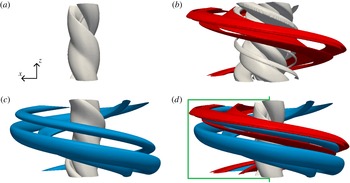
Isovorticity surfaces of (a)
 $|{\it\omega}|=1$
(grey), (b)
 $|{\it\omega}_{r}|=0.03$
(red with green core), (c)
 $|{\it\omega}_{{\it\theta}}|=0.2$
(blue with green core) and (d)
 $|{\it\omega}|,|{\it\omega}_{r}|$
and
 $|{\it\omega}_{{\it\theta}}|$
overlaid (with the core
 ${\it\omega}_{r}$
and
 ${\it\omega}_{{\it\theta}}$
surfaces removed) at
 $T=10.5$
to show the three-dimensional structure of the helical spiral in figure 19. The plane shown in figure 19 is indicated in (d).

The parent filaments in both cases are easily identified in the
 ${\it\omega}_{{\it\theta}}$
contours (figures 17
a–c and 19
a–c) as the filament dipoles and are denoted by
 $\text{P}_{a}$
–
 $\text{P}_{c}$
. Note that the parent filaments are helical (figure 20) and thus do not have a clear head as in the sketch (figure 14). The meridional (
 $r$
–
 ${\it\theta}$
) flow induced by the parent filaments (seen in figure 18 for the first period) tilts the mean axial vorticity into the radial direction, which forms new filaments as radial perturbation vorticity is tilted into the azimuthal direction by the mean strain (offspring filaments, noted by
 $\text{O}_{a}$
–
 $\text{O}_{c}$
). Examining the vorticity contours during both periods, it can be seen that both pairs of offspring filaments decay during the period of renewed production responsible for the slowed energy decay. Additionally, the radii of the offspring filaments in figures 17 and 19 are greater than the radii of renewed turbulent kinetic energy growth in figure 16 (for instance, offspring filaments in figure 19 are located at
 $r\approx 2$
and the region of growing energy is at
 $r\approx 1$
in figure 16
b), indicating that the offspring filaments are not responsible for energy growth. The presence and intensity of the parent–offspring vortices indicates they play an active role in vortex–turbulence interaction, and can potentially generate new growth; however, they are not responsible for the energy production observed here.
Isovorticity contours of (a)
 ${\it\omega}_{{\it\theta}}$
and (b)
 ${\it\omega}_{r}$
(contour increments are
 $|{\it\delta}{\it\omega}|=0.1$
, with fine scales shown by
 $|{\it\delta}{\it\omega}|=0.02$
for
 $|{\it\omega}_{r}|<0.1$
) at
 $T=10.5$
in the axial (
 $x$
–
 $y$
) plane at
 $z=z_{l}/2$
. Shading indicates negative vorticity. The thick red line is
 $|{\it\omega}|=1$
, indicating the vortex core. Viewed from
 $+z$
to
 $-z$
in figure 20.

Radial vorticity,
 ${\it\omega}_{r}$
, contours (figures 17
d–f and 19
d–f) show several important features outside the core. During both periods of production, the generation of the offspring filaments (
 $\text{O}_{a}$
–
 $\text{O}_{c}$
) via the parent filaments (
 $\text{P}_{a}$
–
 $\text{P}_{c}$
) tilting axial vortex lines, as in figure 14(b), can be seen. The radiating vorticity patches within the parent filaments (figure 17
d–f) are a consequence of core dynamics (localized tilting of axial vorticity into radial vorticity). The
 ${\it\omega}_{r}$
contours seen within the core in the axial plane (figure 21
b) suggest that the azimuthal wavenumber doubles, similar to the apparent doubling of the axial wavenumber within the core seen in the meridional plane contours (figures 17
d and 19
d). The importance of the changes to the wavenumbers on the flow evolution are as yet unexplored, but not surprising due to the nonlinear dynamics briefly discussed above.
The vorticity generation due to axial flow –
 ${\it\omega}_{z}^{\prime }$
generated by
 $\partial W/\partial r$
tilting
 ${\it\omega}_{r}^{\prime }$
and
 ${\it\omega}_{r}^{\prime }$
generation by tilting of
 ${\it\Omega}_{{\it\theta}}$
by
 ${\it\omega}_{z}^{\prime }$
(figure 15
a,b) – depends on axial flow near the vortex core (figure 6), which restricts the area to examine for renewed growth in figures 17 and 19. Near the core contour are patches, denoted as
 $\text{A}_{a}{-}\text{A}_{c}$
, of radial (figures 17
d,e and 19
d,e) and azimuthal vorticity (figures 17
a,b and 19
a,b) which intensify during the period of renewed production, and then decay as the energy decreases (figure 13). This intensification is not due to core dynamics – which causes the perturbation vorticity to oscillate out of phase – as both
 ${\it\omega}_{r}^{\prime }$
and
 ${\it\omega}_{{\it\theta}}^{\prime }$
grow simultaneously, indicating vorticity generation due to axial flow and azimuthal swirl (tilting of
 ${\it\omega}_{r}^{\prime }$
to produce
 ${\it\omega}_{{\it\theta}}^{\prime }$
) are responsible for the growth. Vorticity generation due to axial flow ends, and the patches appear to merge with the core fluctuations (compare the distinct
 ${\it\omega}_{{\it\theta}}$
patches marked
 $\text{A}_{b}$
in figures 17
b and 19
b to the distorted core fluctuation marked
 $\text{A}_{c}$
in figures 17
c and 19
c). Additionally, the growing patches of
 ${\it\omega}_{r}$
on the core periphery (
 $\text{A}_{b}$
, figures 17
e and 19
e) are not offspring filaments associated with tilting of mean axial vorticity due to the adjacent patches of
 ${\it\omega}_{{\it\theta}}$
(figures 17
b and 19
b), which would produce oppositely signed
 ${\it\omega}_{r}$
to what is observed. Furthermore, the radii of the vorticity patches
 $\text{A}$
in figures 17 and 19 more closely match the radii where turbulent kinetic energy increases in figure 16. Note that vorticity generation due to axial flow occurs for a large range of
 $q$
(growth for stable
 $q$
values is discussed by Heaton & Peake (Reference Heaton and Peake2007)). Based on vorticity contours and the dynamics discussed earlier herein, the vorticity production and energy growth responsible for the reduced energy decay in figure 13 are caused by the induced axial flow on the vortex column.
Interestingly, even though the
 ${\it\omega}_{{\it\theta}}$
core fluctuations and filaments outside the core (figure 19
a–c) decay after
 $T=11.2$
, axial flow
 $(W_{max})$
continues to increase (figure 8). As the external filaments which drove the initial generation of axial flow are decaying, the merging of the near-core fluctuation (
 $\text{A}$
in figure 19) into the core likely drives this growth. Movement of the core fluctuations and the late-time dynamics can be understood using helical wave decomposition (Melander & Hussain Reference Melander and Hussain1993b
); however such analysis is beyond this work. The axial flow may then become self-sustained by establishing a cycle of near-core vorticity growth (i.e. new
 $\text{A}$
cells) and subsequent merger with the core, which increases axial flow and renews near-core vorticity growth. Combined with vorticity generation outside the core (mean straining and the circulation overshoot, Hussain & Stout Reference Hussain and Stout2013), which can be triggered by the remnants of the filaments, continual generation of axial flow and formation of new vorticity filaments outside the core may occur, which would lead to instability and possibly break up in practical
 $Re$
flows.
7 Concluding remarks
Azimuthal vorticity filaments encircling a vortex column, generated by mean straining of external turbulence, undergo self-induced advection in the radial direction, as well as (primarily) in the axial direction, based on the filaments’ spatial orientation and swirl direction. The self-induced motion of a generic filament with radial and axial vorticities (i.e.
 ${\it\omega}_{r}^{\prime }$
and
 ${\it\omega}_{z}^{\prime }$
, hence any non-axisymmetric filament) is found to have non-negligible radial advection (because of inclination of spiral filaments) leading to induced axial flow within the column (see appendix A). To isolate the axial flow mechanism, a transient growth optimal perturbation is used, which generates filaments that induce axial flow within the vortex without the other complicating dynamics, i.e. pairing, cross-annihilation, etc., seen in vortex–turbulence interaction. This axial flow leads to instability at high
 $Re$
, as revealed by late-time growth of the perturbation. Instability due to turbulence-induced axial flow potentially leads to vortex breakup and accelerated vortex decay – useful for reducing the threat of trailing vortices and improving air traffic safety.
Turbulence-generated axial flow is due to the inherent structure of the filaments wrapped around the vortex, and thus occurs even in vortices with axial flow, i.e. Batchelor vortices. In such a case, the generated axial flow can lead either to instability via increasing
 $W$
or stability by reducing
 $W$
. In a Batchelor vortex, as in a trailing vortex, the axial flow generated by turbulence would develop as a function of the downstream position, leading to a possible stagnation point when the turbulence-generated
 $W$
matches the initially present
 $W$
, i.e. vortex breakdown. The conditions and parameters for breakdown have been heavily discussed for the base flow (see Leibovich Reference Leibovich1978; Schmücker & Gersten Reference Schmücker and Gersten1988, and others); however, including turbulence-induced axial flow potentially improves understanding of the onset and dynamics of vortex breakdown.
There are three areas for future work on this topic, beginning with confirming the observed trends for vortex–turbulence interaction dependent on the initial turbulence intensity. To properly confirm these trends, higher-
 $Re$
simulations (up to and beyond
 $Re=10^{7}$
) are needed, likely through the use of LES. Second is the regenerative perturbation growth on the vortex column, which appears to result from the axial flow reaching the unstable range. Careful examinations of the flow evolution and dynamics are needed to separate (or merge) the influence of axial velocity and the hairpin mechanism of HPS. Third is analysing vortex breakup into turbulence due to the induced axial velocity, where the mean profiles are distinctly different from the Batchelor vortex because of the region of oppositely signed mean axial velocity, necessitated by the constant zero meridional circulation. Additionally, the prospect of destabilizing axial flow generated by fine-scale turbulence in large-scale coherent structures has applications to numerous turbulent flows where large-scale structures appear before transition to turbulence, such as mixing layers, jets, wakes and boundary layers.
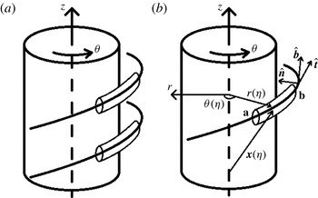
(a) Sketch of filament segments, with the thick line denoting the axes of the filaments. (b) Vortex filament segment, from a to b, defined by the position vector
 $\boldsymbol{x}({\it\eta})=r({\it\eta})\hat{\boldsymbol{r}}+z({\it\eta})\hat{\boldsymbol{z}}$
, with
 ${\it\eta}=0$
at a sketched with tangent
 $(\hat{\boldsymbol{t}})$
, normal
 $(\hat{\boldsymbol{n}})$
and binormal
 $(\hat{\boldsymbol{b}})$
unit vectors.

Appendix A. Generation of axial flow
We consider two segments of weak, parallel vortex filaments of equal and opposite circulations surrounding the vortex column (figure 22
a), and focus on their self-induction. Let the segments be located in the same radius range and assume that they have non-zero radial and axial vorticities. Each segment is located at the position vector
 $\boldsymbol{x}({\it\eta},t)$
(figure 22
b), where
 ${\it\eta}$
is a parameterization from zero (point a) to one (point b) along the segment, and
 $t$
is time (where the time dependence is treated explicitly below). The self-induced motion of the segment is given by Hama (Reference Hama1962):
 $$\begin{eqnarray}\boldsymbol{u}_{\boldsymbol{s}}(\boldsymbol{x})={\it\gamma}{\it\kappa}\ln (L/d)\hat{\boldsymbol{b}}/(4{\rm\pi}),\end{eqnarray}$$
where
 ${\it\gamma}$
is the filament’s circulation,
 $\hat{\boldsymbol{b}}$
is the binormal unit vector,
 ${\it\kappa}$
is the curvature (i.e. inverse of the radius of curvature),
 $L$
is the length, and
 $d$
is the core radius of the segment; the local induction approximation assumes
 $\ln (L/d)=A$
is constant (Callegari & Ting Reference Callegari and Ting1978). From (A 1), two segments with the same
 $\hat{\boldsymbol{b}}$
, i.e. same spatial orientation, but opposite circulations self-advect in opposite directions.
To determine the binormal vector
 $(\hat{\boldsymbol{b}})$
, and hence the components of self-induced advection in cylindrical coordinates
 $(r,{\it\theta},z)$
, write the position vector of point a on the segment axis as
 $\boldsymbol{x}({\it\eta})=r({\it\eta})\hat{\boldsymbol{r}}({\it\theta}({\it\eta}))+z({\it\eta})\hat{\boldsymbol{z}}$
(figure 22
b). Each term of
 $\boldsymbol{x}({\it\eta})$
is expanded as
 $r({\it\eta})=r_{0}+({\rm\Delta}r){\it\eta}+O({\it\eta}^{2}),{\it\theta}({\it\eta})={\it\theta}_{0}+({\rm\Delta}{\it\theta}){\it\eta}+O({\it\eta}^{2})$
and
 $z({\it\eta})=z_{0}+({\rm\Delta}z){\it\eta}+O({\it\eta}^{2})$
, where
 $(r_{0},{\it\theta}_{0},z_{0})$
is the initial position of point a on the segment, namely a in figure 22(a), and
 $({\rm\Delta}r,{\rm\Delta}{\it\theta},{\rm\Delta}z)=(\partial r({\it\eta})/\partial {\it\eta},\partial {\it\theta}({\it\eta})/\partial {\it\eta},\partial z({\it\eta})/\partial {\it\eta})$
along the curve.
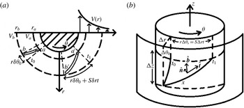
Effect of mean strain on vorticity filaments shown in (a) an end view and (b) an oblique view. Also shown in (b) are
 $(\hat{\boldsymbol{t}},\hat{\boldsymbol{n}},\hat{\boldsymbol{b}})$
and the axial extent of the filament
 $({\rm\Delta}z)$
.

Consider the end view of the segment in figure 23(a), where the radial variation of the mean azimuthal velocity,
 $V$
, moves point a azimuthally by
 ${\it\theta}_{a^{\prime }}-{\it\theta}_{a}={\it\delta}{\it\theta}_{a}=V_{a}t/r_{a}$
over time
 $t$
from the initial time and position and moves point b by
 ${\it\theta}_{b^{\prime }}-{\it\theta}_{b}={\it\delta}{\it\theta}_{b}=V_{b}t/r_{b}$
. The change in the filament’s azimuthal extent is then
 ${\it\delta}{\it\theta}={\it\delta}{\it\theta}_{a}-{\it\delta}{\it\theta}_{b}=V_{a}t/r_{a}-V_{b}t/r_{b}$
. Rewriting this as
 ${\it\delta}{\it\theta}={\it\delta}(V/r)t$
, multiply the right-hand side by
 ${\it\delta}r/{\it\delta}r$
and divide both sides by
 ${\it\delta}{\it\eta}={\it\eta}_{a}-{\it\eta}_{b}$
; we get
 ${\it\delta}{\it\theta}/{\it\delta}{\it\eta}=[{\it\delta}(V/r)/{\it\delta}r]({\it\delta}r/{\it\delta}{\it\eta})t$
. Taking the difference in
 $\text{radius}/{\it\eta}$
to be infinitesimally small, the term inside the brackets becomes a derivative,
 $\partial (V/r)/\partial r$
, and
 ${\it\delta}r,{\it\delta}{\it\theta}$
become
 ${\rm\Delta}r,{\rm\Delta}{\it\theta}$
. Then,
 ${\rm\Delta}{\it\theta}=[r\partial (V/r)/\partial r][{\rm\Delta}r]t=r^{-1}[r\partial (V/r)/\partial r][{\rm\Delta}r]t=r^{-1}[{\rm\Delta}r]St$
, where
 $r\partial (V/r)/\partial r=S$
, the mean strain rate (figure 23
b, where the change in (
 ${\rm\Delta}r,{\rm\Delta}{\it\theta},{\rm\Delta}z$
) is sketched). Note that this also follows from the fact that a vortex line is a material line in inviscid flows, whereby the inviscid azimuthal generation of vorticity (discussed in PH06) equates to the azimuthal lengthening of a material line, i.e.
 ${\it\omega}_{{\it\theta}}={\it\omega}_{r}St$
is equivalent to
 $r[{\rm\Delta}{\it\theta}_{s}]=[{\rm\Delta}r]St$
. This is in addition to the initial azimuthal variation from a to b along the segment,
 ${\rm\Delta}{\it\theta}_{0}$
; thus the total
 ${\rm\Delta}{\it\theta}={\rm\Delta}{\it\theta}_{0}+{\rm\Delta}{\it\theta}_{s}$
. Note that the radial
 $({\rm\Delta}r)$
and axial
 $({\rm\Delta}z)$
variations of the filament are constant, i.e. there is no generation of radial or axial vorticity, and the generation of azimuthal variation due to the strain accounts for the time dependence of
 $\boldsymbol{x}({\it\eta},t)$
.
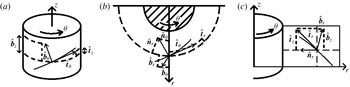
Decomposition of
 $(\hat{\boldsymbol{t}},\hat{\boldsymbol{n}},\hat{\boldsymbol{b}})$
in (a) a
 ${\it\theta}$
–
 $z$
plane (a cylinder coaxial with the vortex column); (b) in an
 $r$
–
 ${\it\theta}$
plane (looking down the
 $z$
axis); and (c) in an
 $r$
–
 $z$
plane. Note that
 $\hat{\boldsymbol{n}}$
lies in the
 $r$
–
 ${\it\theta}$
plane, with
 $\hat{\boldsymbol{n}}_{{\it\theta}}$
omitted from (a) for clarity.

To calculate the binormal unit vector, the tangent and normal vectors are first calculated from the position vector,
 $\boldsymbol{x}$
; the individual components of the three unit vector are sketched in figure 24. The derivatives of the unit vectors are
 $\dot{\hat{\boldsymbol{r}}}=\partial \hat{\boldsymbol{r}}/\partial {\it\eta}=(\partial \hat{\boldsymbol{r}}/\partial {\it\theta})(\partial {\it\theta}/\partial {\it\eta})=\hat{{\bf\theta}}\dot{{\it\theta}}$
and
 $\dot{\hat{{\bf\theta}}}=\partial \hat{{\bf\theta}}/\partial {\it\eta}=(\partial \hat{{\bf\theta}}/\partial {\it\theta})(\partial {\it\theta}/\partial {\it\eta})=-\hat{\boldsymbol{r}}\dot{{\it\theta}}$
, where dots indicate derivatives with respect to
 ${\it\eta}$
. The (un-normalized) tangent vector is
 $\boldsymbol{t}={\dot{r}}\hat{\boldsymbol{r}}+r\dot{{\it\theta}}\hat{{\bf\theta}}+{\dot{z}}\hat{\boldsymbol{z}}$
; the (un-normalized) normal vector is
 $\boldsymbol{n}=(\ddot{r}-r\dot{{\it\theta}}^{2})\hat{\boldsymbol{r}}+(2{\dot{r}}\dot{{\it\theta}}+r\ddot{{\it\theta}})\hat{{\bf\theta}}+\ddot{z}\hat{\boldsymbol{z}}$
. As the second derivatives are small,
 $\ddot{r}$
and
 $\ddot{z}$
are ignored. The curvature,
 ${\it\kappa}=|\boldsymbol{n}|$
, is
 $r_{c}\dot{{\it\theta}}^{2}$
using order of magnitude analysis and assuming
 $r\approx r_{c}$
, where
 $r_{c}$
is the radius of point a. The components of the binormal unit vector
 $(\hat{\boldsymbol{b}})$
, calculated by taking
 $\boldsymbol{t}\times \boldsymbol{n}$
and normalizing, are
 $$\begin{eqnarray}\displaystyle & \displaystyle \hat{\boldsymbol{b}}\boldsymbol{\cdot }\hat{\boldsymbol{r}}=-2[{\rm\Delta}r][{\rm\Delta}z](r_{c}^{-1}[{\rm\Delta}r]St)/|\hat{\boldsymbol{b}}|, & \displaystyle\end{eqnarray}$$
 $$\begin{eqnarray}\displaystyle & \displaystyle \hat{\boldsymbol{b}}\boldsymbol{\cdot }\hat{{\bf\theta}}=-(r_{c}+[{\rm\Delta}r]{\it\eta})(r_{c}^{-1}[{\rm\Delta}r]St)^{2}{\rm\Delta}z/|\hat{\boldsymbol{b}}|,\quad \text{and} & \displaystyle\end{eqnarray}$$
 $$\begin{eqnarray}\displaystyle & \displaystyle \hat{\boldsymbol{b}}\boldsymbol{\cdot }\hat{\boldsymbol{z}}=[[{\rm\Delta}r]^{2}({\it\theta}_{0}+r_{c}^{-1}[{\rm\Delta}r]St\,{\it\eta})+(r_{c}+[{\rm\Delta}r]{\it\eta})^{2}(r_{c}^{-1}[{\rm\Delta}r]St)^{3}]/|\hat{\boldsymbol{b}}|, & \displaystyle\end{eqnarray}$$
where
 ${\rm\Delta}{\it\theta}_{0}$
is neglected and
 $|\hat{\boldsymbol{b}}|\approx r_{c}^{2}(r_{c}^{-1}[{\rm\Delta}r]St)^{3}$
, based on order of magnitude approximations. Combining (A 1) and (A 2), the self-induced radial velocity becomes
 $$\begin{eqnarray}\boldsymbol{u}_{\boldsymbol{s}}\boldsymbol{\cdot }\hat{\boldsymbol{r}}=-{\it\gamma}A[{\rm\Delta}r][{\rm\Delta}z]/[2{\rm\pi}r_{c}^{3}(r_{c}^{-1}[{\rm\Delta}r]St)^{4}].\end{eqnarray}$$
Integration of (A 5) in time gives
 $$\begin{eqnarray}\displaystyle r_{f} & {\approx} & \displaystyle r_{c}+{\it\gamma}Ar_{c}[{\rm\Delta}r][{\rm\Delta}z]/[6{\rm\pi}([{\rm\Delta}r]S)^{4}t^{3}]-{\it\gamma}Ar_{c}[{\rm\Delta}r][{\rm\Delta}z]/[6{\rm\pi}([{\rm\Delta}r]S)^{4}t_{0}^{3}]\nonumber\\ \displaystyle & {\approx} & \displaystyle r_{0}+{\it\gamma}Ar_{c}[{\rm\Delta}r][{\rm\Delta}z]/[6{\rm\pi}([{\rm\Delta}r]S)^{4}t^{3}],\end{eqnarray}$$
where
 $r_{0}$
combines
 $r_{c}$
and the contribution from the initial time considered,
 $t_{0}$
. To illustrate this, consider a space curve,
 $\boldsymbol{x}({\it\eta})$
, as shown in figure 25(a), with
 ${\rm\Delta}r<0$
and
 ${\rm\Delta}z>0$
. For a filament with
 ${\it\gamma}>0$
(figure 25
b, top filament), it radially advects outwards (as well as in the
 $+z$
direction) between
 $t_{0}$
and
 $t_{1}$
; similarly, a filament with
 ${\it\gamma}<0$
(figure 25
b, bottom filament) radially advects inwards (and in the
 $-z$
direction).
(a) Vorticity filament segment with
 ${\rm\Delta}r<0$
and
 ${\rm\Delta}z>0$
at
 $t_{0}$
with
 $(\hat{\boldsymbol{t}},\hat{\boldsymbol{n}},\hat{\boldsymbol{b}})$
shown. Note that
 $\hat{\boldsymbol{b}}$
is in
 $(+r,+z)$
direction. (b) Advection of a filament at
 $t_{1}$
with
 ${\it\gamma}_{1}>0$
(upper), in the direction of the binormal, and
 ${\it\gamma}_{2}<0$
(lower), in the opposite direction of the binormal.

The axial velocity at the axis induced by a filament (approximated as a ring),
 $W_{f}$
, is given by
 $$\begin{eqnarray}W_{f}=-{\it\gamma}/(2r_{f}).\end{eqnarray}$$
Let
 ${\it\delta}r_{f}={\it\gamma}Ar_{c}[{\rm\Delta}r][{\rm\Delta}z]/[6{\rm\pi}([{\rm\Delta}r]S)^{4}t^{3}]$
. Note that by treating the filament as a vortex ring, the effect of
 ${\it\omega}_{r}$
on
 $W_{f}$
is neglected, which simplifies the derivation. The total induced axial flow for two filaments with the same spatial orientation but opposite circulations is
 $$\begin{eqnarray}\displaystyle W_{tot} & = & \displaystyle W_{f}(r_{1})+W_{f}(r_{2})\nonumber\\ \displaystyle & = & \displaystyle -{\it\gamma}/(2r_{0}+2{\it\delta}r_{f})+{\it\gamma}/(2r_{0}-2{\it\delta}r_{f})\nonumber\\ \displaystyle & = & \displaystyle [-{\it\gamma}(r_{0}-{\it\delta}r_{f})+{\it\gamma}(r_{0}+{\it\delta}r_{f})]/[2(r_{0}+{\it\delta}r_{f})(r_{0}-{\it\delta}r_{f})]\nonumber\\ \displaystyle & = & \displaystyle (2{\it\gamma}{\it\delta}r_{f})/(2\{r_{0}^{2}-[{\it\delta}r_{f}]^{2}\})\nonumber\\ \displaystyle & = & \displaystyle \{{\it\gamma}^{2}Ar_{c}[{\rm\Delta}r][{\rm\Delta}z]/[6{\rm\pi}([{\rm\Delta}r]S)^{4}t^{3}]\}/\{r_{0}^{2}+{\it\gamma}^{2}A^{2}r_{c}^{2}[{\rm\Delta}r]^{2}[{\rm\Delta}z]^{2}/[6{\rm\pi}([{\rm\Delta}r]S)^{4}t^{3}]^{2}\}\nonumber\\ \displaystyle & = & \displaystyle \{6{\rm\pi}{\it\gamma}^{2}Ar_{c}[{\rm\Delta}r][{\rm\Delta}z]([{\rm\Delta}r]S)^{4}t^{3}\}/\{r_{0}^{2}[6{\rm\pi}([{\rm\Delta}r]S)^{4}t^{3}]^{2}+{\it\gamma}^{2}A^{2}r_{c}^{2}[{\rm\Delta}r]^{2}[{\rm\Delta}z]^{2}\}.\nonumber\\ \displaystyle & & \displaystyle\end{eqnarray}$$
At early times,
 $t$
is small, and the first term in the denominator of (A 8),
 $r_{0}^{2}[6{\rm\pi}([{\rm\Delta}r]S)^{4}t^{3}]^{2}$
, is small compared to the second term. Then, the early time growth of
 $W_{tot}$
is
 $$\begin{eqnarray}W_{tot}=[6{\rm\pi}{\it\gamma}^{2}([{\rm\Delta}r]S)^{4}t^{3}]/[{\it\gamma}^{2}Ar_{c}[{\rm\Delta}r][{\rm\Delta}z]]\sim t^{3}.\end{eqnarray}$$
The effects of strain, seen in the curvature and binormal vector, would dominate the growth of
 $W_{tot}$
; the cubic rate matches the linear analysis above in this paper (extended from PH06).
From this analysis, the generic behaviour of all filaments is to undergo both axial and radial self-advection; hence any pair of inclined filaments will radially separate and generate axial flow. The only exception will be axisymmetric filaments, which undergo no radial drift, as the binormal vector is purely axial. As filaments generated from turbulence have arbitrary inclinations, this analysis proves useful in understanding the source of axial flow.
The above analysis assumes only two, thin, weak vortex filaments; for the case of non-constant core radius filaments, the local induction approximation changes due to the non-constant
 $\ln (L/d)$
. Furthermore, approximating the axial velocity as that generated by a vortex ring neglects the effects of
 ${\it\omega}_{r}$
and
 ${\it\omega}_{z}$
in the calculation of
 $W$
using (A 7); the contributions of those two terms reduce the actual growth rate of
 $W$
(figure 8). In the case of vortex–turbulence interaction, non-negligible initial azimuthal variation,
 ${\rm\Delta}{\it\theta}_{0}$
, can delay generation of
 $W_{tot}$
since the filaments may need to be wrapped before radially advecting. Other deviations in the derivation lead to reductions in the estimated
 $W_{tot}$
, such as: significant second-order variation in
 $\boldsymbol{x}({\it\eta})$
, which changes the derivation of (
 $\hat{\boldsymbol{t}}$
,
 $\hat{\boldsymbol{n}}$
,
 $\hat{\boldsymbol{b}}$
); formation of a filament dipole, which causes mutual induction to overwhelm self-induced advection; and viscous cross-annihilation of counter-rotating filaments, which reduces
 ${\it\gamma}$
.