NOMENCLATURE
- N
spool speed, r/min
 ${w_f}$
fuel flow, lbm/s
- x
state vector
- u
control input
- y
output vector
- $\rho $
scheduling variable
- r
reference trajectory
- e
error
- z
auxiliary output
- $\gamma $
performance index
- Pamb
ambient total pressure
- Rline
iteration variable
- PR
iteration variable
- T2
total temperature of the engine inlet
- P2
total pressure of the engine inlet


Subscripts
- c
closed system
- r
reference
- s
incremental linear system
- 0
equilibrium point
Superscripts
- $ \cdot $
derivative

1.0 INTRODUCTION
Linear control theory is still widely applied in the design of turbojet engine control systems, and an adequately accurate linear model is required to design a well-performing controller(Reference Reberga, Henrion, Bernussou and Vary1). In the framework of linear control theory, the most common approach is to develop switched linear systems or/and linear parameter-varying (LPV) models to achieve the desired fidelity. Many studies have validated such linear procedures. Bruzelius et al.(Reference Yan, Zhao and Liu2) applied an LPV model-based gain scheduling design to a turbofan engine and obtained a controller with good performance. Sui et al.(Reference Chen and Zhao3) first proposed a system identification method based on an equilibrium manifold expansion model, and further developed an equilibrium manifold expansion model of LPV form that showed good modelling accuracy(Reference Bruzelius, Breitholtz and Pettersson4). Zhao et al.(Reference Sui and Yu5) investigated a feedback linearisation control method for aeroengines. Furthermore, Shi et al.(Reference Yu, Zhao, Xu, Sui and Liu6) investigated the switching control problem for turbojet engines based on a switched equilibrium manifold expansion model. Chen et al.(Reference Zhao, Liu and Yu7) also designed a switching controller with safety protection based on an equilibrium manifold expansion model. Liu et al.(Reference Liu, Du, Sun, Richter and Zhu8) developed a switched LPV model and achieved robust tracking control of turbojet engine rotor speed.
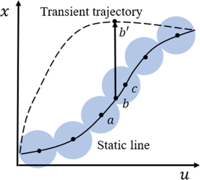
Generally, the linear coefficients of these models are all derived by linearisation at a set of equilibrium points. In fact, the validity of these models is ensured near the equilibria where the linearisation is performed. However, linear models can only provide an approximate description of the engine’s state when the system operates away from equilibrium(Reference Chung Gi-Yun, Prasad, Dhingra and Meisner9,Reference Johansen, Hunt, Gawthrop and Fritz10) . This approximate description is illustrated in Fig. 1, where the system’s actual trajectory is denoted by the dashed line, and the static line is denoted by a solid line. Theoretically, when a turbojet engine operates in the state denoted by point  $b'$, its true linear coefficient is the slope of the trajectory at point
 $b'$. However, in previous linearisation procedures, the linear coefficient may be approximated by the slope of the static line at point b. On at least one occasion, the linear coefficient is approximated by the slopes of the static line at points a and c in an LPV model that is built based on the equilibrium manifold of the system.
Schematic diagram of equilibrium linearization.

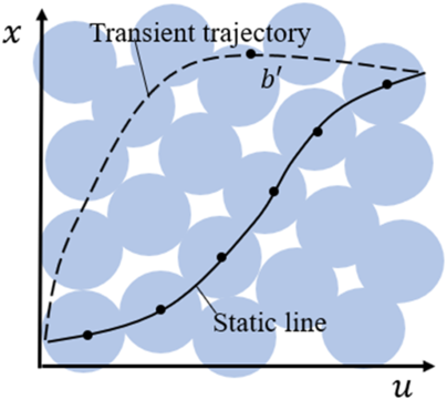
In this sense, it is necessary to develop a more accurate linear model to ensure its fidelity in transient or off-equilibrium states. The general problem behind this concrete problem can be defined as an off-equilibrium linearisation problem. Previously, Chung et al.(Reference Chung Gi-Yun, Prasad, Dhingra and Meisner9) proposed an analytical linearisation method where the model can be linearised at each state along the transient trajectory. This method is only feasible and accurate if the object can be described by sets of algebraic expressions, and it also leads to a tedious and complicated procedure. Johansen et al.(Reference Johansen, Hunt, Gawthrop and Fritz10) proposed an off-equilibrium linearisation method to improve the transient performance and verified its feasibility. Leith et al.(Reference Leith and Leithead11) proposed velocity-based linearisation techniques to transform a nonlinear system into LPV form based on every operating point. These two methods are actually based on the same mathematical theory and can develop an accurate LPV system for every operating point of a nonlinear system; For example, suppose that the turbojet engine still operates in the state denoted by point  ${\rm{b'}}$ as shown in Fig. 2
 ${\rm{b'}}$, then its linear coefficient can be determined by its own states described by the parameters x and u. In these procedures, linear models can adequately capture the system dynamics near both on- and off-equilibrium states.
Schematic diagram of off-equilibrium linearization.

In the framework of linear control theory, in addition to linearisation procedures, LPV control is another important topic that has been widely used as a reliable alternative to gain scheduling control for nonlinear systems. The most common forms of the LPV model are the polytope LPV model and affine parameter-dependent model. The polynomial form can provide a close approximation if the whole range of operating conditions has surface features, and in fact, the operating conditions of turbojet engines meet this requirement. Wilfried et al.(Reference Gilbert, Henrion, Bernussou and Boyer12) used a polynomial transfer function for the modelling objects and fixed-order controllers, which can be successfully applied to turbofan engines. Feng et al.(Reference Lu, Qian, Huang and Qiu13) developed an in-flight adaptive turbofan engine model using a polynomial LPV approach. For the polynomial LPV model, the controller design problem can be transformed into an SOS programming problem, which can be solved using many existing software packages. Wu et al.(Reference Wu and Prajna14) proposed an SOS-based approach for the analysis and control synthesis of an LPV system with a polynomial state space. Papachristodoulou et al.(Reference Papachristodoulou and Papageorgiou15) analysed the robust stability and robust performance of a polynomial quasi-LPV model by using SOS techniques, and this method was applied to an aircraft model. Those studies have demonstrated the feasibility of the combination of a polynomial LPV model and SOS programming.
It is suggested herein that the linearisation should be carried out not only at equilibrium states but also in off-equilibrium operating regimes. This will result in a global approximation to the engine state, regardless of whether equilibrium or off-equilibrium. Theoretically, the transient control performance can be improved by introducing such off-equilibrium linearisation-based control. Subsequently, a gain scheduling control procedure based on the off-equilibrium linearisation models is proposed by using sum-of-squares (SOS) programming. This paper is organised as follows: Firstly, the off-equilibrium linearisation model of a turbojet engine is provided. Subsequently, the control framework of the LPV controller and SOS constraints are introduced. Finally, the application of the control procedures to a turbojet engine is presented, as well as corresponding simulation results.
2.0 OFF-EQUILIBRIUM LINEARISATION AND LPV MODELLING
2.1 Off-equilibrium linearisation method
Consider the nonlinear system
 \begin{align}\left\{\begin{array}{l} \dot x = f( {x,u}) \\[3pt] y = g( {x,u}) \end{array} \right. \end{align}
The equilibrium manifold of this system is given by
 \begin{align}{ {em = \left\{ {({x,u})|\,f({x,u}) = 0} \right\}} } \end{align}
The traditional equilibrium linearisation is defined at each equilibrium point  $\left( {{x_0},{u_0}} \right) \in em$ as
 \begin{align}\dot x &= f( {{x_0} + \delta x,{u_0} + \delta u{\rm{}}}) \nonumber\\[3pt] &= f( {{x_0},{u_0}}) + {{\partial f} \over {\partial x}}{\Big|_{\left( {{x_0},{u_0}} \right)}}\delta x + {{\partial f} \over {\partial u}}{\Big|_{\left( {{x_0},{u_0}} \right)}}\delta u + H \cdot O \cdot T \nonumber\\[3pt] &\approx A\delta x + B\delta u \\[-18pt]\nonumber\end{align}
Equilibrium linearisation is popular because of the wide application of analysis of local stability properties at equilibrium points. However, in fact, the system can be linearised about every arbitrary point  $( {\tilde{x},\tilde{u} })$, as shown below
 \begin{align}\dot x &= f( {\tilde{x}+ \delta x,\tilde{u}+ \delta u{\rm{}}}) \nonumber\\[3pt] &= f( {\tilde{x},\tilde{u}}) + {{\partial f} \over {\partial x}}{\Big|_{\left( {\tilde{x},\tilde{u}} \right)}}\delta x + {{\partial f} \over {\partial u}}{\Big|_{\left( {\tilde{x},\tilde{u}} \right)}}\delta u + H \cdot O \cdot T \nonumber\\[3pt] &\approx {\dot {\tilde{x}}}+ A\delta x + B\delta u \end{align}
This equation can also be written as
 \begin{align}{ {\delta \dot x = A\delta x + B\delta u} } \end{align}
where  $\delta x = x - \tilde{x}$ and
 $\delta u = u - \tilde{u}$.
For the transient dynamics of a turbojet engine, the system changes step by step. In this work, the engine model is linearised about every point within the operating region. Therefore, the nonlinear system (1) can be transformed into LPV form as
 \begin{align} \left\{ \begin{array}{l} {{\dot{x}_s}}= {A_s}(\rho){x_s} + {B_s}(\rho){u_s}\\[3pt] \mathop {{\dot y_s} = }{C_s}(\rho){x_s} + {D_s}(\rho){u_s} \end{array} \right. \end{align}
where  ${x_s} = {\rm{}}\delta x = x - \tilde{x}(\rho)$,
 ${u_s} = {\rm{}}\delta u = u - \tilde{u}(\rho)$,
 ${y_s} = {\rm{}}\delta y = y - \tilde{y}(\rho)$. The reference points
 $\left[ {\tilde{x}(\rho),\tilde{u}(\rho),\tilde{y}(\rho)} \right]$ and linear coefficients
 ${A_s}(\rho),{\rm{}}{B_s}(\rho),{\rm{}}{C_s}(\rho),{\rm{}}{D_s}(\rho)$ are determined by the measurable variables
 $\rho $, which is subject to the following sets:
 $$\Phi = \{ \rho |{g_i}(\rho) \ge 0,i = 1,2, \cdots \cdot \cdot \cdot ,l\} $$
This LPV model (6) is linearised at every point and determined along the transient trajectory, thus resulting in more linear models within the operating region.
2.2 Off-equilibrium linearisation model of turbojet engine
The proposed linearisation approach requires a nonlinear engine model to build an input–output function. This nonlinear turbojet engine model can be described as follows:
 \begin{align} \left\{ \begin{array}{l}\dot n = f({n,{w_f}})\\[3pt] y = g({n,{w_f}}) \end{array}\right. \end{align}
The expressions of f and g are described by compressor maps and turbine maps, which contain lookup tables and empirical data. In practice, such models are difficult to describe as an LPV model using analytical transformations. The convergence of the nonlinear model is achieved by the flow conservation equation, and the solver iterates until the flow error terms achieve the desired tolerance(Reference Chapman, Lavelle, May, Litt and Guo16). The spool speed n is updated iteratively by the integration of engine dynamics  $\dot n$ as
 \begin{align}{ {n = \smallint \!\dot n} } \end{align}
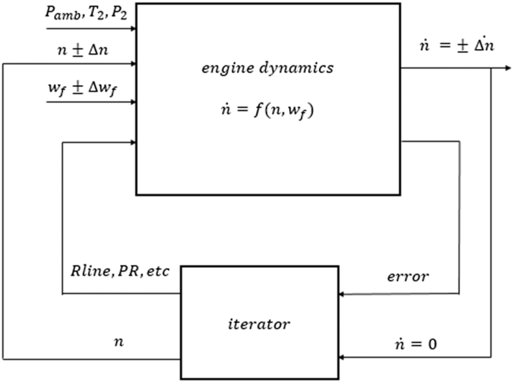
Firstly, consider the common equilibrium linearisation approach(Reference Seldner and Cwynar17,Reference Sugiyama18) . If the turbojet engine is at steady-state points, one can apply small perturbations to the states and inputs, respectively, resulting in the changes  $\Delta \dot n{|_{\Delta n}}$ and
 $\Delta \dot n{|_{\Delta {w_f}}}$ for the engine in Fig. 3. The linear coefficients can be obtained as shown below:
 \begin{align} \left\{ \begin{array}{l} {A = {\dfrac{\Delta \dot n{|_{\Delta n}}}{\Delta n}}} \\ \\[-5pt] {B = {\dfrac{\Delta \dot n{|_{\Delta {w_f}}}}{\Delta {w_f}}}} \end{array} \right. \end{align}
Steady states of turbojet engines.

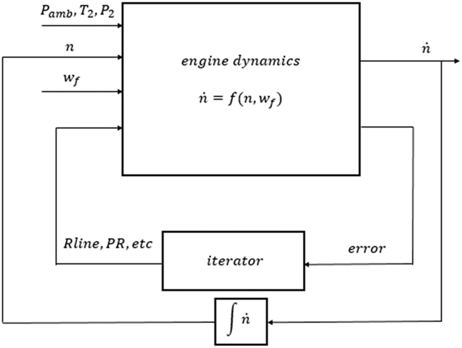
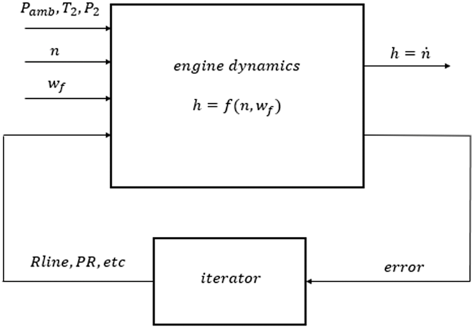
Subsequently, we use the simulation model shown in Fig. 4 to perform the off-equilibrium linearisation. Since the basic concept of linearisation is to approximate the function  $f({n,{w_f}})$ with a linear function, and the approximation is performed in the framework of algebraic equations, we delete the integrator of the simulation model in Fig. 4 as shown in Fig. 5. We thus obtain the input–output function for linearisation as
 \begin{align}{ {h = f({n,{w_f}})} } \end{align}
where n and  ${w_f}$ are independent variables and
 $h = \dot n$ is a dependent variable.
This function is often composed of a data interpolation of compressor and turbine maps, which means that it is influenced by measurement noise. In this case, the small perturbation method may be unable to ensure accuracy locally in a practical application. However, the function (10) may still have a low-dimensional property globally, and we can use the polynomial fitting method to approximate this function, so the fitting function will remain smooth over small scales.
Transient states of turbojet engines.

Input–output function for linearization of turbojet engines.

For example, one can use the high-order polynomial functions  $p({n,{w_f}})$ and
 $q({n,{w_f}})$ to fit
 $f({n,{w_f}})$ and
 $g({n,{w_f}})$, respectively, according to
 \begin{align} \left\{ \begin{array}{l} {min\mathop \sum \nolimits_k \left\|p\big( {{n^k},w_f^k} \big) - f\big( {{n^k},w_f^k}\big)\right\|} \\ \\[-7pt] {min\mathop \sum \nolimits_k \left\|q\big( {{n^k},w_f^k} \big) - g\big( {{n^k},w_f^k} \big)\right\|}\end{array} \right. \end{align}
where  $\big( {{n^k},w_f^k} \big)$ is the kth data point, and the majority of these points are off-equilibrium points. Then, the linear coefficients of the LPV model (6) can be obtained as follows:
 \begin{align}\left\{ \begin{array}{l}{{A_s}({n,{w_f}}) = \dfrac{{\partial p({n,{w_f}})} }{ {\partial n}}} \\ \\[-7pt] {{B_s}({n,{w_f}}) = \dfrac{{\partial p({n,{w_f}})}}{ {\partial {w_f}}}} \\ \\[-7pt] {{C_s}({n,{w_f}}) = \dfrac{{\partial q({n,{w_f}})}}{ {\partial n}}} \\ \\[-7pt] {{D_s}({n,{w_f}}) = \dfrac{{\partial q({n,{w_f}})} }{ {\partial {w_f}}}} \end{array} \right. \end{align}
This method can not only ensure the accuracy of the linearisation, but also ensure the smoothness of the input–output function (10).
3.0 GAIN SCHEDULING CONTROLLER DESIGN USING SOS PROGRAMMING
3.1 Augmented system and control framework
Consider the tracking problem of  ${\mathcal{H}_\infty }$ control, where
 ${y_r}$ is the tracking trajectory. The actual reference for the model is
 \begin{align}{ {r = {y_r} - {\tilde{y}_r}} } \end{align}
where  ${\;\tilde{y}_r}$ is the value of
 ${y_r}$ in the last step. The output error is described as
 \begin{align}{ {e = r - {y_s}} } \end{align}
Add  ${x_e} = \smallint \!e$ as an augmented state to make the system error-free for the steady state. Select the output error e and weighted input
 $\beta {u_s}$ as the auxiliary output z. The augmented system then has the form
 \begin{align} \left\{ \begin{array}{l} {\dot x = A(\rho)x + {B_1}(\rho)r + {B_2}(\rho)u} \\ \\[-7pt] {z = {C_1}(\rho)x + {D_{11}}(\rho)r + {D_{12}}(\rho)u} \end{array} \right. \end{align}
where
 \begin{align*} x &= \left[\begin{array}{l} {{x_s}} \\ {{x_e}} \end{array}\right],\,\,\, u = {u_s},\,\,\, z = \left[ \begin{array}{c} e \\ {\beta {u_s}} \end{array} \right],\,\,\, A(\rho) = \left[ \begin{array}{c@{\quad}c} A_s (\rho) & 0 \\ - {C_s}(\rho) & 0 \end{array} \right],\,\,\, {B_1}(\rho) = \left[ \begin{array}{l} 0 \\ I \end{array} \right],\\[3pt] {B_2}(\rho) &= \left[ \begin{array}{c} {{B_s}(\rho)} \\ { - {D_s}(\rho)} \end{array} \right],\,\,\, {C_1}(\rho) = \left[ \begin{array}{c@{\quad}c} { - {C_s}(\rho)} &0 \\ 0 & 0 \end{array} \right],\,\,\, {D_{11}}(\rho) = \left[ \begin{array}{l} I \\ 0 \end{array} \right],\,\,\, {D_{12}}(\rho) = \left[ \begin{array}{c} { - {D_s}(\rho)} \\ {\beta I} \end{array} \right] \end{align*}
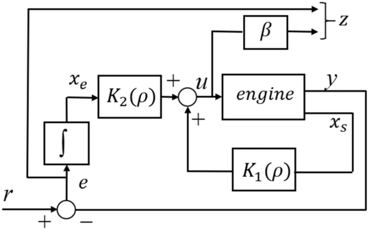
In this paper, the state feedback control strategy is used to track the reference trajectory
 \begin{align}{ {u = \left[ {{ {{K_1}(\rho)}\ {{K_2}(\rho)} } } \right]x} }\end{align}
Let  $K(\rho) = \left[ {{ {{K_1}(\rho)}\ {{K_2}(\rho)} } } \right]$, then the closed-loop system of the turbojet engine in Fig. 6 can be described as
 \begin{align} \left\{ \begin{array}{l} {\dot x = {A_c}(\rho)x + {B_c}(\rho)r} \\ \\[-7pt] {z = {C_c}(\rho)x + {D_c}(\rho)r} \end{array} \right. \end{align}
where
 \begin{align*}{A_c}(\rho) &= A(\rho) + {B_2}(\rho)K(\rho), {B_c}(\rho) = {B_1}(\rho), \\[3pt] {C_c}(\rho) &= {C_1}(\rho) + {D_{12}}(\rho)K(\rho), {D_c}(\rho) = {D_{11}}(\rho) \end{align*}
The engine in closed loop.

3.2 LPV gain scheduling controller design
This section introduces a practically valid controller design method for state-feedback synthesis by using the bounded real lemma and SOS programming.
Lemma 1 Lemma 1(Reference Xie19) For the transfer function  $G( s ) = \left( {A,B,C,D} \right)$, it follows that
 ${G_\infty } < \gamma $ and matrix A is stable, if and only if there exists a symmetric positive-definite matrix P that satisfies
 \begin{align} \left[ \begin{array}{c@{\quad}c@{\quad}c} {AP + P{A^T}} & {P{C^T}} & B \\ {CP} & { - I} & D \\ {{B^T}} & {{D^T}} & { - {\gamma ^2}I} \end{array} \right]
< 0 \end{align}
where the symmetric positive matrix P is usually called the Lyapunov function matrix. This lemma is the famous bounded real lemma.
Notation.  $\mathbb{R}[ x ]$ denotes the set of polynomials in x with real coefficients. The subset
 ${\rm{\Sigma }}[ x ]: = \left\{ {\pi \in \mathbb{R}[ x ]:\pi = \pi _1^2 + \pi _2^2 + \cdots + \pi _m^2,{\pi _1}, {\cdots}\,,{\pi _m} \in \mathbb{R}[ x ]} \right\}$ of
 $\mathbb{R}[ x]$ is the set of SOS polynomials.
 ${{\rm{\Sigma }}_m}[ x ]$ denotes the matrix whose elements are SOS polynomials in x.
Lemma 2: Lemma 2(Reference Topcu, Packard, Seiler and Wheeler20) Given  ${g_0},{g_1},{\cdots}\,,{g_m} \in \mathbb{R}[ x ]$, if there exist
 ${S_1},{\cdots}\,,{S_m} \in {{\rm{\Sigma }}_m}[ x]$ such that
 ${g_0} - \mathop \sum \limits_{i - 1}^m {S_i}{g_i} \in {{\rm{\Sigma }}_m}[ x ]$, then
 $\left\{ {x \in {\mathcal{R}^n}:{g_i}( x ) \ge 0,i = 1, {\cdots}\,,m} \right\} \subseteq \{ x \in {\mathcal{R}^n}:{g_0}( x ) > 0\} $.
Theorem 1: Theorem 1Consider a general tracking control structure of the LPV system (7), then a parameter-dependent state feedback controller  $u(\rho) = K(\rho)x$, achieving the given
 ${\mathcal{H}_\infty }$ performance index
 $\gamma > 0$ and stability of the closed-loop system for
 $\rho \in \Phi = \{ \rho |{g_i}(\rho) \ge 0,\break i = 1,2, \cdots \cdot \cdot \cdot ,l\} $, is given by
 $K(\rho) = M(\rho){P^{ - 1}}$ where
 $P = {P^T} > 0$, with
 ${S_i}(\rho)$,
 $M(\rho)$ and P satisfying
 \begin{align}{ {L(\rho) - \mathop \sum \limits_{i = 1}^l {S_i}(\rho){g_i}(\rho) \in {{\rm{\Sigma }}_m}[ x ]} } \end{align}
 \begin{align}{ {{S_i}(\rho) \in {{\rm{\Sigma }}_m}[x ],i = 1, {\cdots}\,,l} } \end{align}
where
 \begin{align*}L(\rho) = - \left[ \begin{array}{c@{\quad}c@{\quad}c} \begin{array}{c}{A(\rho)P + {B_2}(\rho)M(\rho)} \\\\[-7pt] { + P{A^T}(\rho) + {M^T}(\rho)B_2^T(\rho)} \end{array} & {\rm{*}} & {\rm{*}} \\\\[-7pt] {B_1^T(\rho)} & { - I} & {\rm{*}} \\\\[-7pt] {{C_1}(\rho)P + {D_{12}}(\rho)M(\rho)} & {{D_{11}}(\rho)} & { - {\gamma ^2}I} \end{array} \right]\end{align*}
Proof From the given Equations (19) and (20) and Lemma 2, we have
 $$L(\rho) > 0$$
which can be written as
 \begin{align*} \left[ \begin{array}{c@{\quad}c@{\quad}c} \begin{array}{c}{A(\rho)P + {B_2}(\rho)M(\rho)} \\ \\[-7pt] { + P{A^T}(\rho) + {M^T}(\rho)B_2^T(\rho)} \end{array} & {\rm{*}} & {\rm{*}} \\ \\[-7pt] {B_1^T(\rho)} & { - I} & {\rm{*}} \\\\[-7pt] {{C_1}(\rho)P + {D_{12}}(\rho)M(\rho)} & {{D_{11}}(\rho)} & { - {\gamma ^2}I} \end{array} \right]
< 0\end{align*}
for  $\rho \in \Phi = \left\{ {\rho {\rm{|}}{g_i}(\rho) \ge 0,i = 1,2, \cdots \cdot \cdot \cdot ,l} \right\}$.
Let  $K(\rho) = M(\rho){P^{ - 1}}$, then
 \begin{align*}\left[ \begin{array}{c@{\quad}c@{\quad}c} \begin{array}{l}{A(\rho)P + {B_2}(\rho)M(\rho)} \\\\[-7pt] { +P{A^T}(\rho) + {M^T}(\rho)B_2^T(\rho)} \end{array} & {\rm{*}} & {\rm{*}} \\\\[-7pt] {B_1^T(\rho)} & { - I} & {\rm{*}} \\\\[-7pt] {{C_1}(\rho)P + {D_{12}}(\rho)M(\rho)} & {{D_{11}}(\rho)} & { - {\gamma ^2}I} \end{array} \right]
< 0,\end{align*}
which results in
 \begin{align*}\left[ \begin{array}{c@{\quad}c@{\quad}c} {{A_c}(\rho)P + P{A^T}(\rho)} & {\rm{*}} & {\rm{*}}\\ \\[-7pt] {B_c^T(\rho)} & { - I} & {\rm{*}} \\ \\[-7pt] {{C_c}(\rho)P} & {{D_c}(\rho)} & { - {\gamma ^2}I} \end{array} \right]
< 0\end{align*}
for  $\rho \in \Phi = \{ \rho |{g_i}(\rho) \ge 0,i = 1,2, \cdots \cdot \cdot \cdot ,l\} $, where
 ${A_c}(\rho) = A(\rho) + {B_2}(\rho)K(\rho)$, and the closed system has the form of Equation (18).
From Lemma 1, we have that the parameter-dependent state matrix  ${A_c}(\rho)$ is stable with guaranteed
 ${\mathcal{H}_\infty }$-gain bound
 $\gamma $. This completes the proof of theorem 1.
Remark 1. Remark 1Using Theorem 1, an LPV controller that satisfies the given  ${\mathcal{H}_\infty }$ performance index
 $\gamma $ of the form of Equation (15) is obtained. Minimising
 $\gamma $ according to Theorem 1 is an optimisation problem with SOS constrains. This problem is also a standard SOS programming problem, which can be solved using many software packages.
4.0 CONTROLLER DESIGN
4.1 LPV modelling
The nonlinear model of the turbojet engine that we used here is from T-MATS developed by NASA(Reference Chapman, Lavelle, May, Litt and Guo16). The input parameter is the fuel flow  ${w_f}$, while the output parameters are the spool speed n and the compressor pressure ratio. In this work, we focus on the validity of the methods, choosing the spool speed as the state parameter as well as the output parameter. However, there are no limitations in the framework on the use of additional states, inputs or outputs. Therefore, the transient states of an engine can be described by
 ${w_f}$ and n, which are often measurable(Reference Jaw and Mattingly21). Because these two variables can determine the changes of system states directly, we choose
 ${w_f}$ and n as determining variables.
 \begin{align} {\tilde \rho }= {\left[ {{ n\ \ {{w_f}} } } \right]^T}.\end{align}
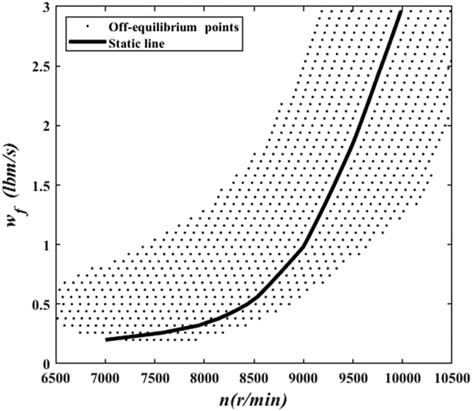
To obtain the LPV model of the nonlinear model, the foregoing linearisation method for the turbojet engine will be used. By performing the input–output function of the engine as shown in Fig. 5, the operating region can be described by 988 points as shown in Fig. 7. The steady-state operation is described by the black line, while the majority of the black dots are off-equilibrium points.
Operating region.

To obtain a less conservation solution when solving the SOS programming problem in Theorem 1, it is preferable to have the same orders of magnitude for the determining variables. Therefore,  $\tilde{\rho}$ can be transformed into
 $\rho $ by using the affine transformation as shown below:
 \begin{align} \rho = \left[ \begin{array}{c}{{n_s}} \\ {{w_{fs}}} \end{array} \right] = \left[ \begin{array}{c@{\quad}c} {\dfrac{1}{{1990}}} &0 \\ \\[-7pt] 0 & {\dfrac{5}{7}} \end{array} \right]\tilde{\rho}+ \left[ \begin{array}{c} {{\dfrac{851}{199}}} \\ \\[-7pt] {\dfrac{8 }{ 7}} \end{array} \right] \end{align}
The operating region can be described by the following set
 \begin{align}{ {\Gamma = \left\{ {\rho \in \mathbb{R} {^2}|{g_i}(\rho) \ge 0{\rm{}},i = 1,{\cdots}\,,4{\rm{}}} \right\}} } \\[-20pt]\nonumber\end{align}
where
 \begin{align}\left\{ \begin{array}{@{}l} {{g_1}(\rho) = 1 - n_s^2} \\ \\[-7pt] {{g_2}(\rho) = 1 - w_{fs}^2} \\ \\[-7pt] {{g_3}(\rho) = {{\left( {{n_s} + 1.15} \right)}^2} + {{\left( {{w_{fs}} - 1.15} \right)}^2} - 3.31} \\ \\[-7pt] {{g_4}(\rho) = 4.345 - {{\left( {{n_s} + 0.98} \right)}^2} + {{\left( {{w_{fs}} - 0.93} \right)}^2}} \end{array} \right.\end{align}
In this region, the input–output function clearly has surface features. Therefore, we can fit this function by a third-order polynomial  $p(\rho)$, and the fitting result is accurate enough. The linear coefficients, which are second-order polynomials, can be obtained as follows:
 \begin{align}\left[ \begin{array}{l} {{A_s}(\rho)} \\ \\[-7pt] {{B_s}(\rho)} \end{array} \right] &= \left[ \begin{array}{c@{\quad}c} \dfrac{1 }{{1990}} & 0 \\ \\[-7pt] 0 & {\dfrac{5 }{ 7}} \end{array} \right]\left[ \begin{array}{l} {\dfrac{{\partial p(\rho)}}{ {\partial {n_s}}}} \\ \\[-7pt] {\dfrac{{\partial p(\rho)} }{ {\partial {w_{fs}}}}} \end{array} \right] \nonumber\\[6pt] & = \left[ \begin{array}{c} { - 0.7113 - 0.483{n_s} - 0.2396{w_{fs}} - 0.2516n_s^2 + 0.8967{n_s} \cdot {w_{fs}} - 0.2744w_{fs}^2} \\ \\[-7pt] {543.1 + 238.9{n_s} - 412.9{w_{fs}} - 51.33n_s^2 + 297.7{n_s} \cdot {w_{fs}} + 144.7w_{fs}^2} \end{array} \right]\end{align}
 \begin{align}\left[ \begin{array}{l}{{C_s}(\rho)} \\ \\[-7pt] {{D_s}(\rho)} \end{array} \right] = \left[ \begin{array}{l}1 \\\\[-7pt] 0 \end{array}\right] \end{align}
The LPV model based on the proposed off-equilibrium linearisation method (OE-LPV) will have the form of Equation (6)
 \begin{align*}\left\{ \begin{array}{l} {{{\dot x_s}}= {A_s}(\rho){x_s} + {B_s}(\rho){u_s}} \\\\[-7pt] {{{\dot y_s}}= {C_s}(\rho){x_s} + {D_s}(\rho){u_s}} \end{array}\right.\end{align*}
where
 \begin{align*}{x_s} = \delta n = n - \tilde{n}(\rho),{u_s} = \delta u = u - {{\dot w_f}}(\rho),{y_s} = \delta y = y - \tilde{y}(\rho)\end{align*}
and  $\tilde{n}(\rho), {{\dot w_f}}(\rho),\tilde{y}(\rho)$ are determined by the scheduling variable
 $\rho $ respectively.
4.2 Open-loop validation
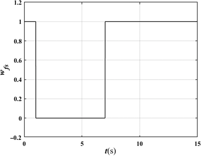
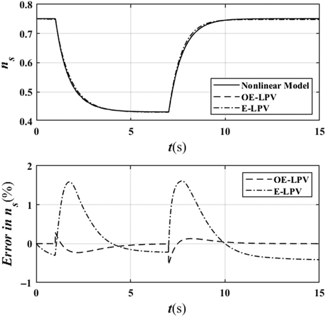
The LPV model can be validated by using different transient trajectories. In this paper, the model is validated by step input in the open-loop system at a sea level static condition and compared with the equilibrium linearisation method-based LPV model (E-LPV), whose linear coefficients are also fitted by second-order polynomials and determined by  ${n_s}$. The step input
 ${w_{fs}}$ is presented in Fig. 8, and the results for the two models are presented in Fig. 9.
Step input.

Step response and error of spool speed.

For the systems with the same input, the error of the off-equilibrium linearisation-based LPV model is much lower than the error of the equilibrium linearisation-based LPV model. The maximum error in the E-LPV is seen to be more than four times that of the OE-LPV model. Furthermore, the steady-state error in the E-LPV is about 0.4%, while that of the OE-LPV is close to 0%.
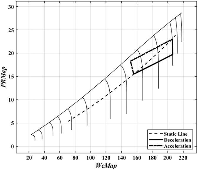
The transient trajectory of the step input on the compressor map is shown in Fig. 10, where the transient operations are clearly away from the static line. In these off-equilibrium conditions, the OE-LPV can capture large transient dynamics more accurately. Therefore, it is concluded that the proposed LPV model based on the off-equilibrium linearisation method achieved a much lower modelling error for depicting the open-loop dynamic behaviour of the example nonlinear engine model considered in this paper.
The transient trajectory of step input on compressor map.

4.3 Controller parameters and simulation results
The proposed LPV model in the open-loop system can achieve higher fidelity. However, a control-oriented model should also be validated in the controller design. Two systems whose open-loop dynamics are similar may exhibit different system behaviour when the system is closed using the same controller(Reference Vinnicombe22). In this section, similar controllers are designed for the two LPV models using the same foregoing control framework with SOS programming.
By solving the SOS programming to minimise the  ${\mathcal{H}_\infty }$ performance index
 $\gamma $ according to Theorem 1, the minimum
 $\gamma $ for the OE-LPV model is 1.01, which means that the obtained tracking robustness of the controller for OE-LPV model has low conservativeness. The symmetric positive matrix P and gain scheduling controller
 $K(\rho)$ for the OE-LPV model is given by
 \begin{align*} K(\rho) = \left[ \begin{array}{l} { - 0.1315 - 0.0652{n_s} + 0.0181{w_{fs}} - 0.0060n_s^2 - 0.0523{n_s} \cdot {w_{fs}} - 0.0164w_{fs}^2} \\\\[-7pt] {0.1013 + 0.0512{n_s} - 0.0141{w_{fs}} - 0.0049n_s^2 + 0.0402{n_s} \cdot {w_{fs}} + 0.0124w_{fs}^2} \end{array} \right]^T\end{align*}
To validate the controllers for the two LPV models and compare their performance, numerical simulations are performed on the nonlinear model. The desired trajectory of the spool speed is as follows:
 \begin{align}{ {{y_r} = {n_0} + \Delta n\left( {1 - {e^{ - {t \over \tau }}}} \right)} }\end{align}
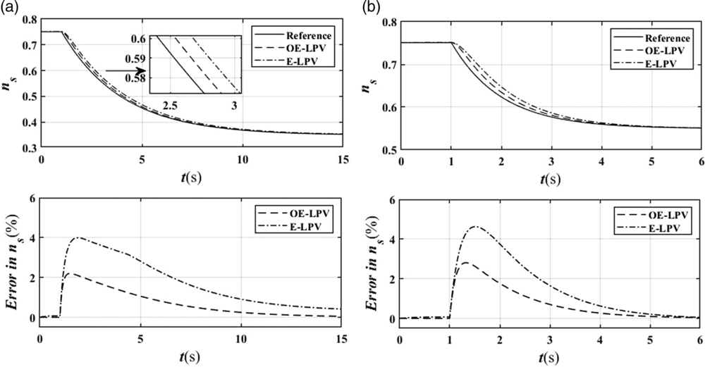
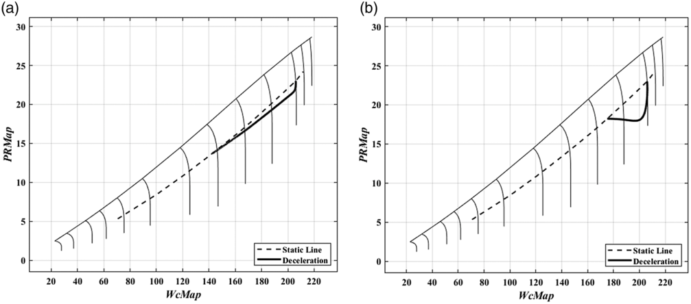
The results for the two different controllers are presented in Fig. 11, and the desired trajectories on the compressor map are shown in Fig. 12. In the first case, the deceleration is at a low velocity, which means that the transient operation is close to the static line, whereas in the second case, the variation is at a high speed, which means that the transient operations are far away from the static line. In both cases, the controller designed using the off-equilibrium linearisation model can track the desired trajectory better than that using the traditional equilibrium linearisation model. An obvious explanation is that the OE-LPV model is more accurate than the E-LPV model whether the trajectories are away from the static line or not.
Nonlinear simulation for tracking n. a) Near static line b) Far from static line.

Desired trajectories of spool speed on the compressor map. a) Near static line b) Far from static line.

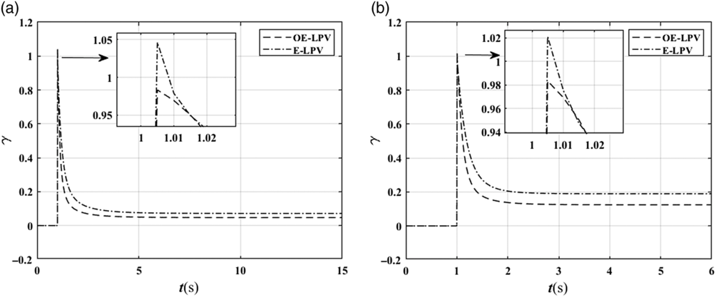
Additionally, the variations of the performance index  $\gamma $ are shown in Fig. 13. It can be seen that the
 $\gamma (t) = \sqrt {{{\mathop \smallint \nolimits_0^\infty {z^T}\left( t \right)z\left( t \right)dt} \over {\mathop \smallint \nolimits_0^\infty {r^T}\left( t \right)r\left( t \right)dt}}} $ value of the closed-loop system in the two cases gradually becomes smaller and eventually much less than 1.01 when using the designed
 ${\mathcal{H}_\infty }$ controller. Under the two transient operations, the performance index
 $\gamma $ of the controller designed using the OE-LPV model is always smaller than that using the E-LPV model, further indicating that the tracking robustness of the present controller offers better performance. Note that the two controllers are designed using the same control framework and the performance of the controllers is similar. However, the benefits seen with the use of the proposed OE-LPV model are still obvious and are expected to become even greater when the LPV models are more complicated.
Changes of performance index  $\gamma $. a) Near static line b) Far from static line.

5.0 CONCLUSION
An off-equilibrium linearisation-based nonlinear control procedure for a turbojet engine with sum-of-squares programming is proposed. Within this control framework, the polynomial LPV model linearised at on- and off-equilibrium conditions is more accurate than the conventional LPV model linearised at only equilibrium conditions, which is demonstrated by the smaller model errors. Furthermore, gain scheduling controllers are designed by solving the SOS programming problem for the two LPV models. The results validate the effectiveness of both the proposed LPV modelling method and the controller design method. The proposed methods thus enable the development of an accurate control-oriented linear model and the design of a well-performing controller. Furthermore, these results motivate further investigation of applications for more complicated turbofan engines.
ACKNOWLEDGMENTS
Financial support from the National Science and Technology Major Project (2017-V-0004-0054) is gratefully acknowledged.