1 Introduction
Flow control is either passive (for example through the modification of a surface profile), or active via actuators. Examples of flow control include the delay of vortex shedding, the reduction of drag and the enhancement of lift (see Gad-el-Hak Reference Gad-el-Hak1996; Gad-el-Hak, Pollard & Bonnet Reference Gad-el-Hak, Pollard and Bonnet2003; Brunton & Noack Reference Brunton and Noack2015, for extensive reviews). In the more specific case of feedback flow control, the actuators rely on sensor readings to adjust their behaviour. Early experimental studies employed ad hoc feedback control schemes. For example, Wehrmann (Reference Wehrmann1965) and Berger (Reference Berger1967) placed a piezoelectric transducer device into an air flow, which served as a cylinder and actuator simultaneously. The transducer was excited by an amplified signal from a hot-wire probe to suppress vortex shedding and delay transition. Similar approaches have been used for feedback flow control, such as cancelling Tollmien–Schlichting waves in a boundary layer with flush-mounted heating elements (Liepmann & Nosenchuck Reference Liepmann and Nosenchuck1982) or delaying the onset of the wake instability in the flow past a cylinder using a loudspeaker (Williams & Zhao Reference Williams and Zhao1989; Roussopoulos Reference Roussopoulos1993).
Subsequent studies have considered some mathematical description of the flow dynamics to implement controllers (see for example Kim & Bewley Reference Kim and Bewley2007; Choi, Jeon & Kim Reference Choi, Jeon and Kim2008; Bagheri et al. Reference Bagheri, Henningson, Hœpffner and Schmid2009; Noack, Morzynski & Tadmor Reference Noack, Morzynski and Tadmor2011; Brunton & Noack Reference Brunton and Noack2015; Taira et al. Reference Taira, Brunton, Dawson, Rowley, Colonius, McKeon, Schmidt, Gordeyev, Theofilis and Ukeiley2017). These mathematical descriptions can be operator based, i.e. derived from the underlying physics, or data based, i.e. derived from numerical or experimental data (Taira et al. Reference Taira, Brunton, Dawson, Rowley, Colonius, McKeon, Schmidt, Gordeyev, Theofilis and Ukeiley2017); and sometimes they use a combination of both operators and data (Reynolds & Hussain Reference Reynolds and Hussain1972).
One can employ a mathematical description to design a suitable feedback controller, test a designed feedback controller before implementing it or both. There are various controller designs available: (i) we can select dynamics for the flow, or we can cancel specific dynamics of the flow, examples of which include pole placement (Litrico & Georges Reference Litrico and Georges1999) and dynamic phasors (Rowley & Juttijudata Reference Rowley and Juttijudata2005; Illingworth, Morgans & Rowley Reference Illingworth, Morgans and Rowley2012); (ii) we can manually tune a controller, examples of which include proportional (Monkewitz Reference Monkewitz1989; Park, Ladd & Hendricks Reference Park, Ladd and Hendricks1993; Son, Jeon & Choi Reference Son, Jeon and Choi2011), proportional–integral (Joshi, Speyer & Kim Reference Joshi, Speyer and Kim1997; Son et al.
Reference Son, Jeon and Choi2011), proportional–derivative (Son et al.
Reference Son, Jeon and Choi2011) and proportional–integral–derivative control (Cohen et al.
Reference Cohen, Siegel, McLaughlin and Myatt2003, Reference Cohen, Siegel, McLaughlin, Gillies and Myatt2005), as well as fuzzy logic control (Cohen et al.
Reference Cohen, Siegel, McLaughlin and Myatt2003, Reference Cohen, Siegel, McLaughlin, Gillies and Myatt2005), and loop shaping (Illingworth Reference Illingworth2014, Reference Illingworth2016); and (iii) we can implement a control scheme which optimises control objectives, while being able to model specific disturbances, examples include
 $H_{2}$
optimal and
 $H_{\infty }$
robust control (Bewley & Liu Reference Bewley and Liu1998; Lauga & Bewley Reference Lauga and Bewley2003, Reference Lauga and Bewley2004), neural network control (Gillies Reference Gillies1998) and model predictive control (Bewley, Moin & Temam Reference Bewley, Moin and Temam2001).
We can improve the performance of feedback flow control by finding the optimal locations for the sensors and actuators employed. Optimal placement is a challenging problem for flow control (and indeed for any control problem) because of the following predicament: we can neither design a controller without placement nor determine the placement performance before designing a controller. Therefore, most placements are based on experience or a flow’s physical characteristics. Åkervik et al. (Reference Åkervik, Hœpffner, Ehrenstein and Henningson2007) placed sensors according to the least stable eigenmode, which provides the best detectability for that mode; and placed actuators according to the least stable adjoint mode, which provides the best stabilisability for that mode. Mons, Chassaing & Sagaut (Reference Mons, Chassaing and Sagaut2017) placed sensors through an adjoint-based sensitivity analysis, which identifies regions most susceptible to changes in initial conditions, boundary conditions or flow parameters. The more specific structural sensitivity was used by Natarajan, Freund & Bodony (Reference Natarajan, Freund and Bodony2016) to place collocated actuator–sensor pairs. Structural sensitivity identifies locations which are ‘characterized by both a high sensitivity of and a strong response in the most unstable mode’ (Schmid & Brandt Reference Schmid and Brandt2014). The region of high structural sensitivity is also known as the wavemaker region, which describes the overlap between eigenmodes and adjoint eigenmodes (Chomaz Reference Chomaz2005; Giannetti & Luchini Reference Giannetti and Luchini2007). Other placement approaches consider the regions where instabilities are present (e.g. Gillies Reference Gillies2001; Bagheri et al. Reference Bagheri, Henningson, Hœpffner and Schmid2009).
While each of these placement approaches is sensible, none of them can alone provide the whole picture concerning the placement problem. To find the optimal placement, one has to first quantify the control performance and then search for the optimal locations (e.g. Chen & Rowley Reference Chen and Rowley2011; Juillet, Schmid & Huerre Reference Juillet, Schmid and Huerre2013; Hu, Morris & Zhang Reference Hu, Morris and Zhang2016). Efficiently searching for the optimal locations originated in the applied mathematics community (see Bensoussan Reference Bensoussan1972; Yu & Seinfeld Reference Yu and Seinfeld1973; Chen & Seinfeld Reference Chen and Seinfeld1975; Kumar & Seinfeld Reference Kumar and Seinfeld1978) where it has been applied to a more general class of distributed-parameter systems (e.g. Burns & King Reference Burns and King1994; Morris Reference Morris2011; Kasinathan & Morris Reference Kasinathan and Morris2013). Recent feedback flow control studies have considered optimal placement for a boundary layer (Belson et al. Reference Belson, Semeraro, Rowley and Henningson2013) and the flow past a cylinder (Akhtar et al. Reference Akhtar, Borggaard, Burns, Imtiaz and Zietsman2015). Related estimation studies investigated optimal placement for the dispersive wave equation (Khan, Morris & Stastna Reference Khan, Morris and Stastna2015), and the Boussinesq equation (Hu et al. Reference Hu, Morris and Zhang2016).
The current work considers the sensor and actuator placement problems for convection-dominated spatially developing flows, such as wall-bounded and free shear flows. These types of flows are subject to spatially varying instabilities, which cause perturbations to be amplified as they are convected downstream (Chomaz, Huerre & Redekopp Reference Chomaz, Huerre and Redekopp1987, Reference Chomaz, Huerre and Redekopp1988, Reference Chomaz, Huerre and Redekopp1990, Reference Chomaz, Huerre and Redekopp1991). Spatially varying instabilities lead to transient growth in stable flows, and to self-sustained oscillations in unstable flows, both of which can be described using hydrodynamic stability theory (Huerre & Monkewitz Reference Huerre and Monkewitz1990; Trefethen et al. Reference Trefethen, Trefethen, Reddy and Driscoll1993; Cossu & Chomaz Reference Cossu and Chomaz1997; Chomaz Reference Chomaz2005). Convection-dominated flows are mathematically characterised by non-orthogonal eigenmodes, which affects the sensor and actuator placement.
One such convection-dominated system suitable for studying the placement problem is the complex Ginzburg–Landau equation (introduced in § 2). It has been the subject of various feedback control studies (e.g. Monkewitz Reference Monkewitz1989; Park et al.
Reference Park, Ladd and Hendricks1993; Lauga & Bewley Reference Lauga and Bewley2003, Reference Lauga and Bewley2004; Cohen et al.
Reference Cohen, Siegel, McLaughlin, Gillies and Myatt2005; Bagheri et al.
Reference Bagheri, Henningson, Hœpffner and Schmid2009; Chen & Rowley Reference Chen and Rowley2011; Colburn Reference Colburn2011; Illingworth Reference Illingworth2015). Since the complex Ginzburg–Landau equation has similar stability characteristics as the Navier–Stokes equations, it can be seen as a computationally less demanding substitute. Chen & Rowley (Reference Chen and Rowley2011, Reference Chen and Rowley2014, Reference Chen and Rowley2015) used the complex Ginzburg–Landau equation to study the optimal placement problem using an
 $H_{2}$
controller. They modified an iterative-gradient minimisation algorithm developed by Hiramoto, Doki & Obinata (Reference Hiramoto, Doki and Obinata2000) to solve for the optimal placement at two stabilities: (i) a system with one unstable mode; and (ii) a transiently unstable system. The optimal placement of up to five sensors and five actuators was considered. For a single sensor and single actuator set-up, neither placement based on the eigenmode and adjoint eigenmode, nor on the wavemaker region, resulted in the optimal solution. It was concluded that placement based on the eigenmodes and adjoint eigenmodes fails because the underlying dynamics is non-normal, and that excessive time lag had a detrimental effect on perturbation control.
The contribution of the current work is to study any trade-offs present when placing a single sensor and a single actuator in the complex Ginzburg–Landau system for a range of stabilities. (The selected stabilities range from stable systems to systems with up to four unstable modes.) We will see that the trade-offs we study become increasingly important as we decrease the stability of the system. This work is significant and timely for flow control: by using a simple system and reducing the number of variables (we only use a single sensor, a single actuator or both), we can show and discuss fundamental trade-offs which make the placement problem a challenging one.
The current work considers three problems, which are defined in § 3 and studied § 4. First, we will look at the placement of a single sensor in the optimal estimation (OE) problem. Second, we will look at the placement of a single actuator in the full-state information control (FIC) problem. This keeps the number of variables small to provide insight into the individual sensor and actuator performances. Third, we will study the combined single sensor and single actuator placement of the input–output control (IOC) problem, which is more applicable to experimental applications. In § 5 we will further analyse the results and discuss the trade-offs which determine the optimal location for a single sensor and single actuator.
2 The complex Ginzburg–Landau equation
This section introduces the linearised complex Ginzburg–Landau equation (CGLE). A comprehensive review of the CGLE is given by Bagheri et al. (Reference Bagheri, Henningson, Hœpffner and Schmid2009). Table 1 summarises the simulation parameters considered in this study (to be introduced), which follow the work of Bagheri et al. (Reference Bagheri, Henningson, Hœpffner and Schmid2009), Chen & Rowley (Reference Chen and Rowley2011) and Oehler, Ooi & Illingworth (Reference Oehler, Ooi and Illingworth2016).
Considered parameters for the CGLE.

2.1 The continuous equation
The linearised CGLE subject to unknown disturbances
 $d(x,t)$
is:
 $$\begin{eqnarray}\displaystyle \frac{\unicode[STIX]{x2202}q(x,t)}{\unicode[STIX]{x2202}t} & = & \displaystyle \left(-\unicode[STIX]{x1D708}\frac{\unicode[STIX]{x2202}}{\unicode[STIX]{x2202}x}+\unicode[STIX]{x1D705}\frac{\unicode[STIX]{x2202}^{2}}{\unicode[STIX]{x2202}x^{2}}+\unicode[STIX]{x1D707}(x)\right)q(x,t)+d(x,t),\end{eqnarray}$$
 $$\begin{eqnarray}\displaystyle & = & \displaystyle Aq(x,t)+d(x,t),\end{eqnarray}$$
 $A$
is the Ginzburg–Landau operator which governs the evolution of the flow’s perturbations
 $q(x,t)$
. The operator is defined on an infinite interval:
 $-\infty <x<\infty$
, with boundary conditions
 $q(x,0)=q_{0}(x)$
and
 $q(x,t)<\infty$
, as
 $x\rightarrow \pm \infty$
. The complex terms
 $\unicode[STIX]{x1D708}=U+2\text{j}c_{u}$
and
 $\unicode[STIX]{x1D705}=1+\text{j}c_{d}$
represent the convective and the dissipative nature of the flow, where
 $U$
is the mean advection velocity,
 $c_{u}$
the most unstable wavenumber and
 $c_{d}$
the dispersion parameter. The overall group velocity of the perturbations is
 $U_{max}=U+2c_{u}c_{d}$
. A parabolic function
 $\unicode[STIX]{x1D707}(x)=\unicode[STIX]{x1D707}_{0}-c_{u}^{2}+\unicode[STIX]{x1D707}_{2}x^{2}/2$
introduces the flow’s non-parallel nature and instabilities, where
 $\unicode[STIX]{x1D707}_{2}<0$
. The flow’s instabilities cause the natural occurrence of amplification when
 $\unicode[STIX]{x1D714}_{i,max}(x)>0$
, and decay when
 $\unicode[STIX]{x1D714}_{i,max}(x)<0$
, where
 $\unicode[STIX]{x1D714}_{i,max}(x)=\unicode[STIX]{x1D707}_{0}+\unicode[STIX]{x1D707}_{2}x^{2}/2$
is the growth rate of the most unstable wavenumber (Chomaz et al.
Reference Chomaz, Huerre and Redekopp1987, Reference Chomaz, Huerre and Redekopp1988; Bagheri et al.
Reference Bagheri, Henningson, Hœpffner and Schmid2009). The natural amplification creates an unstable domain which spans the region:
 $-\sqrt{-2\unicode[STIX]{x1D707}_{0}/\unicode[STIX]{x1D707}_{2}}<x<\sqrt{-2\unicode[STIX]{x1D707}_{0}/\unicode[STIX]{x1D707}_{2}}$
; we refer to the unstable domain’s upstream and downstream limits as
 $X_{I}$
and
 $X_{II}$
.
An analytical solution exists for the complex Ginzburg–Landau equation, from which the eigenvalues (
 $\unicode[STIX]{x1D706}_{n}$
), eigenmodes (
 $\unicode[STIX]{x1D719}_{n}$
), adjoint eigenmodes (
 $\unicode[STIX]{x1D713}_{n}$
) and the wavemaker region (
 $\unicode[STIX]{x1D701}_{n}$
) can be generated:
 $$\begin{eqnarray}\displaystyle & \displaystyle \unicode[STIX]{x1D706}_{n}=\unicode[STIX]{x1D707}_{0}-c_{u}^{2}-\unicode[STIX]{x1D708}^{2}/(4\unicode[STIX]{x1D705})-(n+0.5)h, & \displaystyle\end{eqnarray}$$
 $$\begin{eqnarray}\displaystyle & \displaystyle \unicode[STIX]{x1D719}_{n}(x)=\exp (0.5(\unicode[STIX]{x1D708}x/\unicode[STIX]{x1D705}-(\unicode[STIX]{x1D712}x)^{2}))H_{n}(\unicode[STIX]{x1D712}x), & \displaystyle\end{eqnarray}$$
 $$\begin{eqnarray}\displaystyle & \displaystyle \unicode[STIX]{x1D713}_{n}(x)=\exp (-\bar{\unicode[STIX]{x1D708}}x/\bar{\unicode[STIX]{x1D705}})\bar{\unicode[STIX]{x1D719}}_{n}(x), & \displaystyle\end{eqnarray}$$
 $$\begin{eqnarray}\displaystyle & \displaystyle \unicode[STIX]{x1D701}_{n}(x)=\frac{\unicode[STIX]{x1D719}_{n}(x)\bar{\unicode[STIX]{x1D713}}_{n}(x)}{\langle \unicode[STIX]{x1D719}_{n},\unicode[STIX]{x1D713}_{n}\rangle }, & \displaystyle\end{eqnarray}$$
 $h=\sqrt{-2\unicode[STIX]{x1D707}_{2}\unicode[STIX]{x1D705}}$
,
 $\unicode[STIX]{x1D712}=(-\unicode[STIX]{x1D707}_{2}/(2\unicode[STIX]{x1D705}))^{0.25}$
,
 $n=\{0,1,\ldots \}$
,
 $H_{n}$
is the
 $n$
th Hermite polynomial and
 $\bar{(\cdot )}$
is the complex conjugate. The eigenmodes and adjoint eigenmodes are symmetric with respect to each other. The wavemaker region represents the degree of overlap between the eigenmodes and adjoint eigenmodes (Giannetti & Luchini Reference Giannetti and Luchini2007).
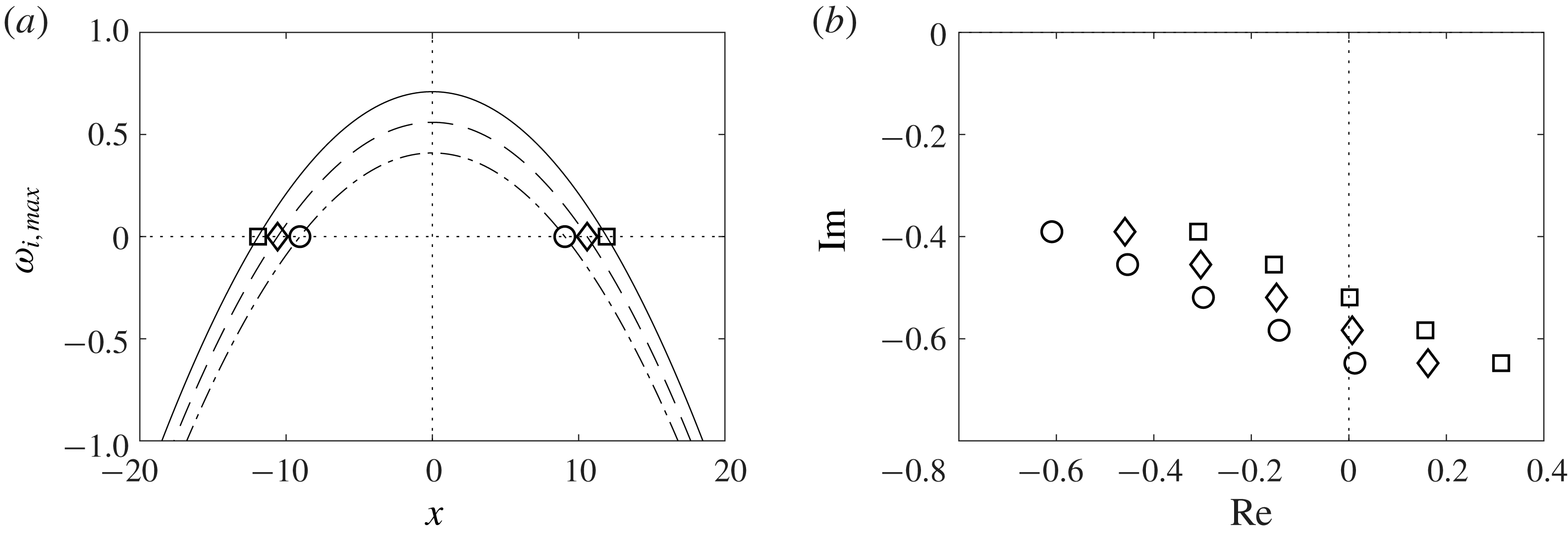
(a) The growth rate of the most unstable wavenumber
 $\unicode[STIX]{x1D714}_{i,max}(x)$
for
 $\unicode[STIX]{x1D707}_{0}$
 $=$
(0.41 (——), 0.56 (– –), 0.71 (– ⋅)), at which
 $X_{II}$
 $=$
(9.1 (○), 10.6 (♢), 11.9 (▫)) and
 $X_{I}=-X_{II}$
. (b) The five most unstable eigenvalues
 $\unicode[STIX]{x1D706}_{n}$
for
 $\unicode[STIX]{x1D707}_{0}$
 $=$
(0.41 (○), 0.56 (♢), 0.71 (▫)).

In § 4 we will consider sensor and actuator placement over a range of
 $\unicode[STIX]{x1D707}_{0}$
, but investigate in more detail only the cases:
 $\unicode[STIX]{x1D707}_{0}=0.41$
,
 $\unicode[STIX]{x1D707}_{0}=0.56$
and
 $\unicode[STIX]{x1D707}_{0}=0.71$
, all of which are globally unstable. These three cases correspond to there being one, two and three unstable modes respectively. We will now look at some characteristics of the CGLE for the three cases. This will become important later when we look at sensor and actuator placement. Figure 1(a) shows the growth rate of the most unstable wavenumber
 $\unicode[STIX]{x1D714}_{i,max}(x)$
, together with the upstream
 $X_{I}$
and downstream
 $X_{II}$
limits of the unstable domain for the three cases; figure 1(b) shows the first five eigenvalues
 $\unicode[STIX]{x1D706}_{n}$
for the three cases. We see that increasing
 $\unicode[STIX]{x1D707}_{0}$
causes
 $\unicode[STIX]{x1D714}_{i,max}(x)$
,
 $X_{I}$
,
 $X_{II}$
and the real part of
 $\unicode[STIX]{x1D706}_{n}$
all to increase in magnitude. However, increasing
 $\unicode[STIX]{x1D707}_{0}$
does not change the shape of the eigenmodes
 $\unicode[STIX]{x1D719}_{n}$
and the shape of the adjoint eigenmodes
 $\unicode[STIX]{x1D713}_{n}$
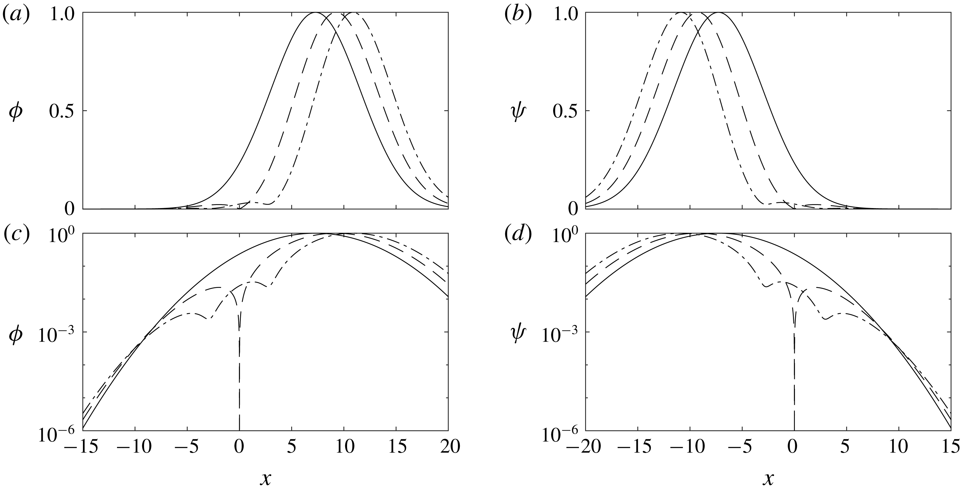
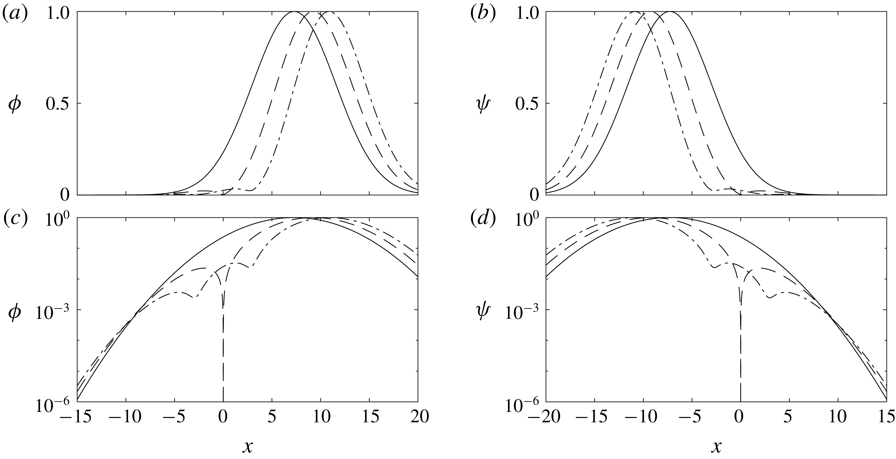
themselves. We have included the three most unstable eigenmodes
 $(\unicode[STIX]{x1D719}_{0},\unicode[STIX]{x1D719}_{1},\unicode[STIX]{x1D719}_{2})$
and adjoint eigenmodes
 $(\unicode[STIX]{x1D713}_{0},\unicode[STIX]{x1D713}_{1},\unicode[STIX]{x1D713}_{2})$
in figure 2. The first three eigenmodes’ global maxima occur at
 $x=7.3$
,
 $x=9.3$
and
 $x=10.9$
. For the second eigenmode
 $\unicode[STIX]{x1D719}_{1}$
a global minimum exists at
 $x=0$
, and for the third eigenmode,
 $\unicode[STIX]{x1D719}_{2}$
, two local minima exist at
 $x\approx -3.0$
and
 $x\approx 2.7$
. Symmetric maxima and minima are obtained for the adjoint eigenmodes.
2.2 The discretised time-invariant model
Until now we have treated the Ginzburg–Landau equation as a continuous system, but to control the flow we need to discretise it and then express it in state-space form. This section describes how to do so.
(a,c) The three most unstable eigenmodes (normalised):
 $\unicode[STIX]{x1D719}_{0}$
(——),
 $\unicode[STIX]{x1D719}_{1}$
(– –), and
 $\unicode[STIX]{x1D719}_{2}$
(– ⋅). (b,d) The three most unstable adjoint eigenmodes (normalised):
 $\unicode[STIX]{x1D713}_{0}$
(——),
 $\unicode[STIX]{x1D713}_{1}$
(– –), and
 $\unicode[STIX]{x1D713}_{2}$
(– ⋅). Figures are on a linear (a,b) and logarithmic (c,d) scale.
The first step is to discretise the operator
 $A$
in the spatial domain, for which we employ the Chebyshev collocation method. We choose an order of
 $N+1=151$
with suitable boundary conditions and scaling
 $L$
, such that the domain is defined between
 $-25<x<25$
. A convergence and scaling study showed convergence for all set-ups considered in this paper. The second step is to discretise the unknown disturbances
 $d(x,t)$
. (More details are given in appendix A.)
Having discretised the continuous CGLE, we can express it as a linear time-invariant state-space model (2.3):

where
 $\boldsymbol{q}$
is the system state and
 $\boldsymbol{z}=\unicode[STIX]{x1D63E}_{z}\boldsymbol{q}$
an output of interest. (For example, we might be interested in
 $\boldsymbol{q}$
at every location in the domain, in which case
 $\unicode[STIX]{x1D63E}_{z}=\unicode[STIX]{x1D644}$
, or only in some smaller region, in which case
 $\unicode[STIX]{x1D63E}_{z}$
will be zero outside the region of interest.) We can combine (2.3) into a single transfer function
 $\unicode[STIX]{x1D64B}(s)$
by taking the Laplace transform.
3 Estimator and controller design
The CGLE is subject to disturbances
 $\boldsymbol{d}$
, which introduce perturbations into the flow. We will first look at how to detect these perturbations using a single sensor placed at
 $x_{s}$
; and second, how to then reduce their effect using a single actuator placed at
 $x_{a}$
. We therefore update the state-space model (2.3) to include an actuator and a sensor (3.1):

The sensor measurement
 $\boldsymbol{y}$
is given by
 $\unicode[STIX]{x1D63E}_{y}\boldsymbol{q}$
, which is contaminated by noise
 $\boldsymbol{n}$
. (We treat
 $\boldsymbol{n}$
as an unknown forcing which is white in space and time with covariance
 $v=\text{E}(\boldsymbol{n}\boldsymbol{n}^{\ast })=10^{-3}$
.) Note that, in general, the quantity we measure (
 $\boldsymbol{y}$
) is not the same as the quantity we want to keep small (
 $\boldsymbol{z}$
). Actuation is represented by
 $\unicode[STIX]{x1D63D}_{u}\boldsymbol{u}$
, which introduces perturbations into the system. The input
 $\boldsymbol{u}$
is also a signal of interest, i.e. something we want to monitor, and therefore
 $\boldsymbol{z}$
includes
 $\boldsymbol{u}$
, which is scaled by
 $\unicode[STIX]{x1D63F}_{u}$
. As in (2.3), we can combine the updated state-space model (3.1) into a single transfer function
 $\unicode[STIX]{x1D64B}(s)$
.
3.1 The estimation and control problems
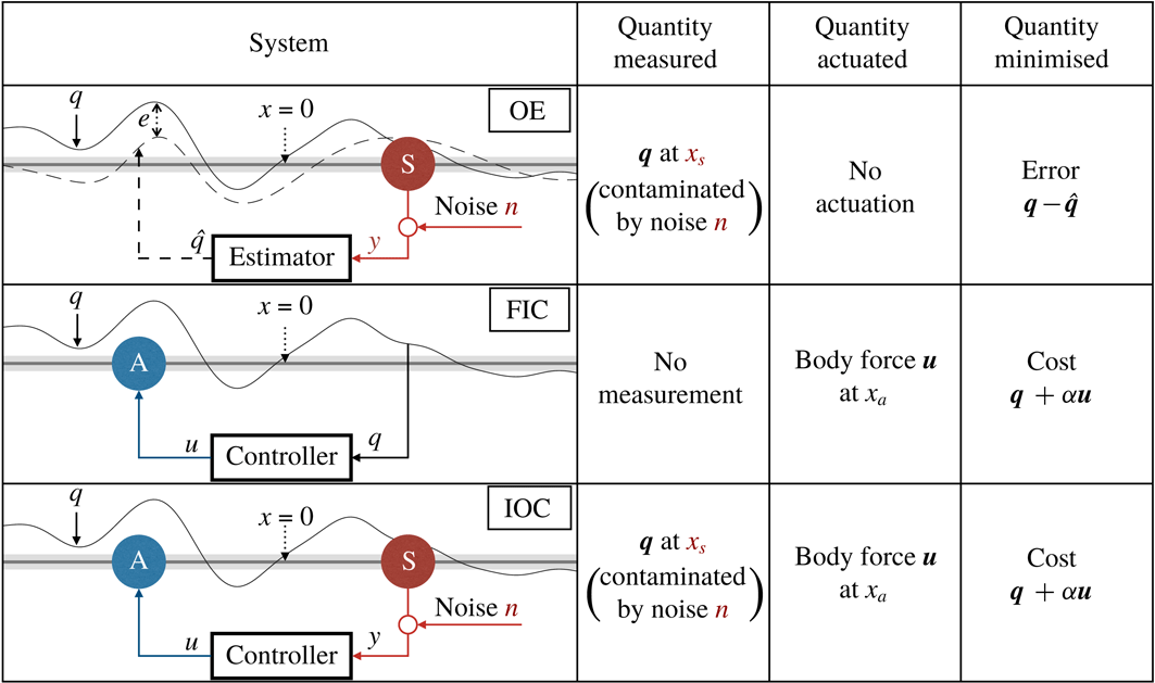
We now want to use the extended plant model (3.1) to investigate three different problems: (i) estimating the entire flow with one sensor (without any control), (ii) controlling the flow with one actuator (when the entire system state is known) and (iii) controlling the flow with one actuator when only provided with a single sensor reading. Figure 3 shows a summary of the three problems. Each problem has a secondary system
 $\unicode[STIX]{x1D64D}(s)$
which needs to be designed (OE: estimator, FIC: controller and IOC: controller.)
Summary of the OE, FIC and IOC problems.
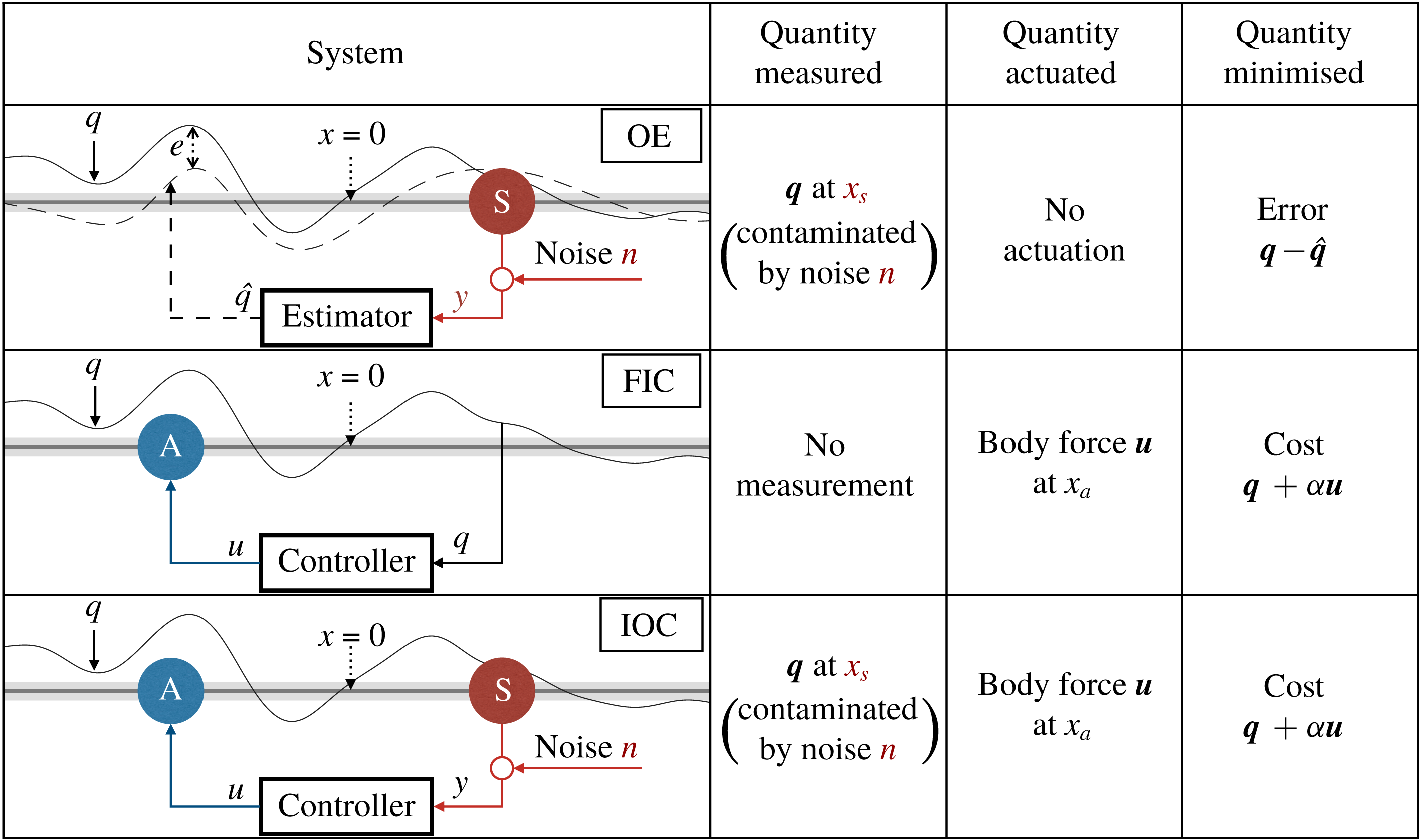
The optimal estimation (OE) problem.
Given a single sensor measurement
 $\boldsymbol{y}$
, which is contaminated by noise
 $\boldsymbol{n}$
, our task in the optimal estimation (OE) problem is to estimate the entire state
 $\boldsymbol{q}$
, which is subject to disturbances
 $\boldsymbol{d}$
. The estimate
 $\hat{\boldsymbol{q}}$
is generated using an estimator. (Thus we only have one sensor to measure the flow; and we want to use it to estimate the flow everywhere.) Our aim is to minimise the estimation error signal
 $\boldsymbol{z}=\boldsymbol{e}$
in the presence of inputs
 $\boldsymbol{d}$
and
 $\boldsymbol{n}$
. The error signal is derived from the cost function:
 $$\begin{eqnarray}\displaystyle J_{OE}=\text{E}\left\{\lim _{t\rightarrow \infty }\frac{1}{T}\int _{0}^{\text{T}}\left(\int _{-\infty }^{\infty }|q(x,t)-\hat{q}(x,t)|^{2}\,\text{d}x\right)\,\text{d}t\right\}. & & \displaystyle\end{eqnarray}$$
The full-state information control (FIC) problem.
Given knowledge of the entire state
 $\boldsymbol{q}$
, our task in the full-state information control (FIC) problem is to control the entire
 $\boldsymbol{q}$
field, which is subject to disturbances
 $\boldsymbol{d}$
, using a single actuator. The actuator force
 $\boldsymbol{u}$
is generated by a controller. (Thus we know everything about the flow; but we only have one actuator to control the flow.) Our aim is to minimise the cost signal
 $\boldsymbol{z}$
in the presence of input
 $\boldsymbol{d}$
. The cost signal
 $\boldsymbol{z}$
is derived from the following cost function:
 $$\begin{eqnarray}J=\text{E}\left\{\lim _{t\rightarrow \infty }\frac{1}{T}\int _{0}^{\text{T}}\left(\int _{-\infty }^{\infty }|q(x,t)|^{2}\,\text{d}x+\unicode[STIX]{x1D6FC}^{2}|u(t)|^{2}\right)\,\text{d}t\right\},\end{eqnarray}$$
where
 $\unicode[STIX]{x1D6FC}$
is a penalisation of the actuator force.
The input–output control (IOC) problem.
Given a single sensor measurement
 $\boldsymbol{y}$
, which is contaminated by noise
 $\boldsymbol{n}$
, our task in the input–output control (IOC) problem is to control the entire
 $\boldsymbol{q}$
field, which is subject to disturbances
 $\boldsymbol{d}$
, using a single actuator. The actuator force
 $\boldsymbol{u}$
is generated by a controller. Full-state information is required for the controller, but since
 $\boldsymbol{q}$
is not available, we estimate it using an estimator. (Thus we only have one sensor to estimate the flow; and we only have one actuator available to control the flow.) Our aim is to minimise the cost signal
 $\boldsymbol{z}$
in the presence of inputs
 $\boldsymbol{d}$
and
 $\boldsymbol{n}$
. The cost signal
 $\boldsymbol{z}$
is derived from (3.3).
3.2 Optimising the performance
We couple the secondary system
 $\unicode[STIX]{x1D64D}(s)$
with the plant model
 $\unicode[STIX]{x1D64B}(s)$
into an overall transfer function
 $\unicode[STIX]{x1D642}(s)$
, defined such that
 $\boldsymbol{z}=\unicode[STIX]{x1D642}(s)\boldsymbol{w}$
. All three stated problems have two things in common: an unknown input
 $\boldsymbol{w}$
(
 $\boldsymbol{d}$
and
 $\boldsymbol{n}$
; or
 $\boldsymbol{d}$
); and an output
 $\boldsymbol{z}$
that we want to keep small. The general design problem can now be stated as follows: given
 $\unicode[STIX]{x1D64B}(s)$
, design
 $\unicode[STIX]{x1D64D}(s)$
such that
 $\unicode[STIX]{x1D642}(s)$
is small. Thus, we first need to quantify the size of
 $\unicode[STIX]{x1D642}(s)$
.

A common way to quantify the size of
 $\unicode[STIX]{x1D642}(s)$
is to use the
 $H_{2}$
-norm, which is defined as:
 $$\begin{eqnarray}\displaystyle \unicode[STIX]{x1D6FE}\triangleq \Vert \unicode[STIX]{x1D642}(s)\Vert _{2}=\sqrt{\frac{1}{2\unicode[STIX]{x03C0}}\int _{-\infty }^{\infty }\text{Trace}[\unicode[STIX]{x1D642}^{\ast }(\text{j}\unicode[STIX]{x1D714})\unicode[STIX]{x1D642}(\text{j}\unicode[STIX]{x1D714})]\,\text{d}\unicode[STIX]{x1D714}}=\sqrt{\frac{1}{2\unicode[STIX]{x03C0}}\int _{-\infty }^{\infty }\mathop{\sum }_{i}(\unicode[STIX]{x1D70E}_{i}(\text{j}\unicode[STIX]{x1D714}))^{2}\,\text{d}\unicode[STIX]{x1D714},}\qquad & & \displaystyle\end{eqnarray}$$
where
 $\unicode[STIX]{x1D70E}_{i}$
are the singular values of
 $\unicode[STIX]{x1D642}(s)$
at frequency
 $\unicode[STIX]{x1D714}$
. Since the singular values can be considered a generalisation of a transfer function’s gain when there are multiple inputs and multiple outputs, we can consider the
 $H_{2}$
-norm as an average gain over all frequencies and all directions. We refer to the
 $H_{2}$
-norm generated by the OE problem as
 $\unicode[STIX]{x1D6FE}_{OE}$
, the FIC problem as
 $\unicode[STIX]{x1D6FE}_{FI}$
and IOC problem as
 $\unicode[STIX]{x1D6FE}_{IO}$
.
The problem of how to then design
 $\unicode[STIX]{x1D64D}(s)$
to make
 $\unicode[STIX]{x1D642}(s)$
small is a well-understood problem, and hence can be solved using standard tools. However, the locations of the sensor and actuator form part of the system
 $\unicode[STIX]{x1D64B}(s)$
, and therefore we can only obtain the best possible
 $\unicode[STIX]{x1D64D}(s)$
for a given sensor location
 $x_{s}$
, a given actuator location
 $x_{a}$
or both. To obtain the optimal sensor and actuator locations we have to either solve
 $\unicode[STIX]{x1D6FE}$
for a set of
 $x_{s}$
and
 $x_{a}$
, known as brute force solving, or use an iterative-gradient minimisation algorithm. We employ an iterative gradient minimisation algorithm which was developed by Chen & Rowley (Reference Chen and Rowley2011), where it was successfully applied to the IOC problem for two values of
 $\unicode[STIX]{x1D707}_{0}$
.
It is important to consider the effect of
 $v$
and
 $\unicode[STIX]{x1D6FC}$
for three reasons: (i) the optimal placement problem, (ii) the estimation performance and (iii) the control performance. Previous studies have looked at the effect of
 $v$
and
 $\unicode[STIX]{x1D6FC}$
for the IOC problem (Lauga & Bewley Reference Lauga and Bewley2004; Chen & Rowley Reference Chen and Rowley2011). Based on these studies we have chosen
 $\unicode[STIX]{x1D6FC}=1/7$
and
 $v=10^{-3}$
. The actuation cost
 $\unicode[STIX]{x1D6FC}$
is a compromise between a reasonably sized actuator signal and an effective reduction in the perturbation magnitude. The noise covariance
 $v$
is a compromise between a negligibly sized sensor noise and the well posedness of the system. The optimal sensor and actuator locations are insensitive to the choice of
 $\unicode[STIX]{x1D6FC}$
and
 $v$
for all systems and
 $\unicode[STIX]{x1D707}_{0}$
considered in this study.
For more information on the estimator design, the controller design and the optimal placement see appendices B and C. Further details on the control tools used in this section (and the appendices) can be found in Kim & Bewley (Reference Kim and Bewley2007), Skogestad & Postlethwaite (Reference Skogestad and Postlethwaite2007), Bagheri et al. (Reference Bagheri, Henningson, Hœpffner and Schmid2009), Aström & Murray (Reference Aström and Murray2010), Chen & Rowley (Reference Chen and Rowley2011).
4 Results
We will now look at optimal placement and the effect that varying the stability of the system has on optimal placement. This section consists of three parts: first, we consider the optimal estimation (OE) problem, then the full-state information control (FIC) problem and finally the input–output control (IOC) problem. We study the OE and FIC problems together for better comparison.
4.1 The OE and FIC problems
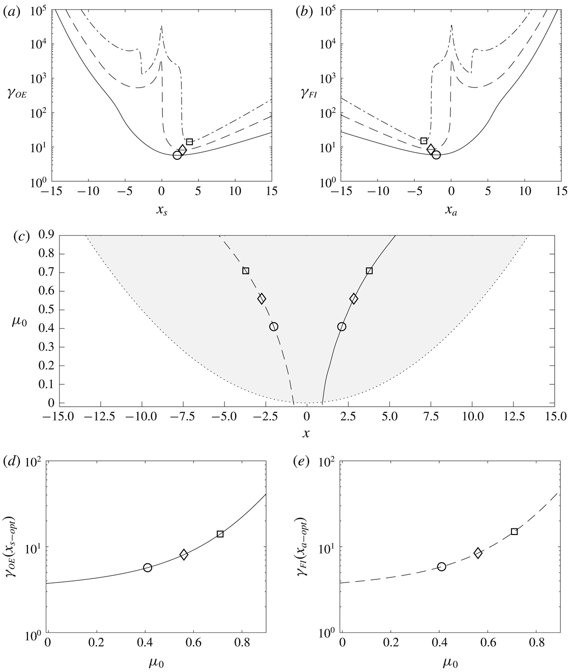
(a) The OE norm
 $\unicode[STIX]{x1D6FE}_{OE}$
as a function of sensor location
 $x_{s}$
and (b) the FIC norm
 $\unicode[STIX]{x1D6FE}_{FI}$
as a function of actuator location
 $x_{a}$
for stability parameters
 $\unicode[STIX]{x1D707}_{0}$
 $=$
(0.41 (——), 0.56 (– –), 0.71; (– ⋅)). (c) The OE optimal sensor location
 $x_{s-opt}$
(——) and the FIC optimal actuator location
 $x_{a-opt}$
(– –), and the unstable domain’s limits (:) as a function of
 $\unicode[STIX]{x1D707}_{0}$
. The unstable domain is shaded grey; it only exists when
 $\unicode[STIX]{x1D707}_{0}>0$
. (d) The OE norm
 $\unicode[STIX]{x1D6FE}_{OE}~(x_{s-opt})$
and (e) the FIC norm
 $\unicode[STIX]{x1D6FE}_{FI}~(x_{a-opt})$
as a function of
 $\unicode[STIX]{x1D707}_{0}$
. (a–e) The optimal locations and energy norms for
 $\unicode[STIX]{x1D707}_{0}$
 $=$
(0.41 (○), 0.56 (♢), 0.71 (▫) are indicated.

We start by looking at the OE problem for a single value of
 $\unicode[STIX]{x1D707}_{0}=0.41$
when random disturbances are applied everywhere in the domain. The estimation error norm
 $\unicode[STIX]{x1D6FE}_{OE}$
is generated as a function of sensor location
 $x_{s}$
in figure 4(a), which reveals the optimal sensor location to be at
 $x_{s-opt}\approx 2.10$
, for which
 $\unicode[STIX]{x1D6FE}_{OE}\approx 5.70$
. Placing the sensor downstream of
 $x_{s-opt}$
is penalised less than placing it upstream of
 $x_{s-opt}$
.
We now repeat the same analysis for the FIC problem. The energy norm
 $\unicode[STIX]{x1D6FE}_{FI}$
is generated as a function of actuator location
 $x_{a}$
in figure 4(b), which reveals the optimal actuator location to be at
 $x_{a-opt}\approx -2.01$
, where
 $\unicode[STIX]{x1D6FE}_{FI}\approx 5.85$
. Analogous to the OE problem, placing the actuator upstream of
 $x_{a-opt}$
is penalised less than placing it downstream of
 $x_{a-opt}$
.
Having found the optimal sensor and actuator locations for a single value of
 $\unicode[STIX]{x1D707}_{0}$
, it is now interesting to look at how placement varies with
 $\unicode[STIX]{x1D707}_{0}$
. Results for two higher values of
 $\unicode[STIX]{x1D707}_{0}$
are also shown figure 4(a,b):
 $\unicode[STIX]{x1D707}_{0}=0.56$
, for which there are two unstable modes, and
 $\unicode[STIX]{x1D707}_{0}=0.71$
, for which there are three unstable modes. When
 $\unicode[STIX]{x1D707}_{0}=0.56$
, the optimal sensor location shifts downstream and
 $\unicode[STIX]{x1D6FE}_{OE}$
increases; a local maximum occurs at
 $x_{s}=0$
and
 $\unicode[STIX]{x1D6FE}_{OE}$
changes rapidly within the vicinity of the maximum. When
 $\unicode[STIX]{x1D707}_{0}=0.71$
, the optimal sensor location shifts even further downstream, and the local maximum at the centre increases in magnitude. Rapid changes of
 $\unicode[STIX]{x1D6FE}_{OE}$
now also occur at
 $x_{s}\approx -3$
and
 $x_{s}\approx 2.7$
(figure 4
a). In all three cases, it is better to place the sensor too far downstream than too far upstream. Similar results are obtained for the FIC problem (figure 4
b).
So far, we considered three distinct values of
 $\unicode[STIX]{x1D707}_{0}$
. We now look in more detail at how
 $x_{s-opt}$
and
 $x_{a-opt}$
vary with
 $\unicode[STIX]{x1D707}_{0}$
; this is computationally expensive, and so we employ the gradient minimisation algorithm of Chen & Rowley (Reference Chen and Rowley2011). Figure 4(c) shows that, as
 $\unicode[STIX]{x1D707}_{0}$
is varied over the range
 $-0.01\leqslant \unicode[STIX]{x1D707}_{0}\leqslant 0.9$
,
 $x_{s-opt}$
shifts downstream from
 $0.92$
to
 $5.36$
, while
 $x_{a-opt}$
shifts upstream from
 $-0.80$
to
 $-5.34$
. In addition to plotting
 $x_{s-opt}$
and
 $x_{a-opt}$
with
 $\unicode[STIX]{x1D707}_{0}$
, it is also interesting to look at the optimal positions’ energy norms, which provide information on the difficulty of estimation and control. In figure 4(d,e) the optimal OE energy norm
 $\unicode[STIX]{x1D6FE}_{OE}(x_{s-opt})$
and the optimal FIC energy norm
 $\unicode[STIX]{x1D6FE}_{FI}(x_{a-opt})$
are shown as a function of
 $\unicode[STIX]{x1D707}_{0}$
. Over the chosen range
 $\unicode[STIX]{x1D6FE}_{OE}$
increases from
 $3.7$
to
 $41.3$
, and
 $\unicode[STIX]{x1D6FE}_{FI}$
increases from
 $3.8$
to
 $45.9$
.
It is now insightful to see how contributions to those norms are distributed throughout the domain. To do so, we use the root-mean-square (r.m.s.) value
 $\unicode[STIX]{x1D716}$
(see appendix D and Bagheri et al.
Reference Bagheri, Henningson, Hœpffner and Schmid2009), defined such that
 $$\begin{eqnarray}\displaystyle \unicode[STIX]{x1D6FE}^{2}=\int _{-\infty }^{\infty }\unicode[STIX]{x1D716}^{2}(x)\,\text{d}x. & & \displaystyle\end{eqnarray}$$
The term
 $\unicode[STIX]{x1D716}_{OE}$
shows the effect of the estimation error on
 $\unicode[STIX]{x1D6FE}_{OE}$
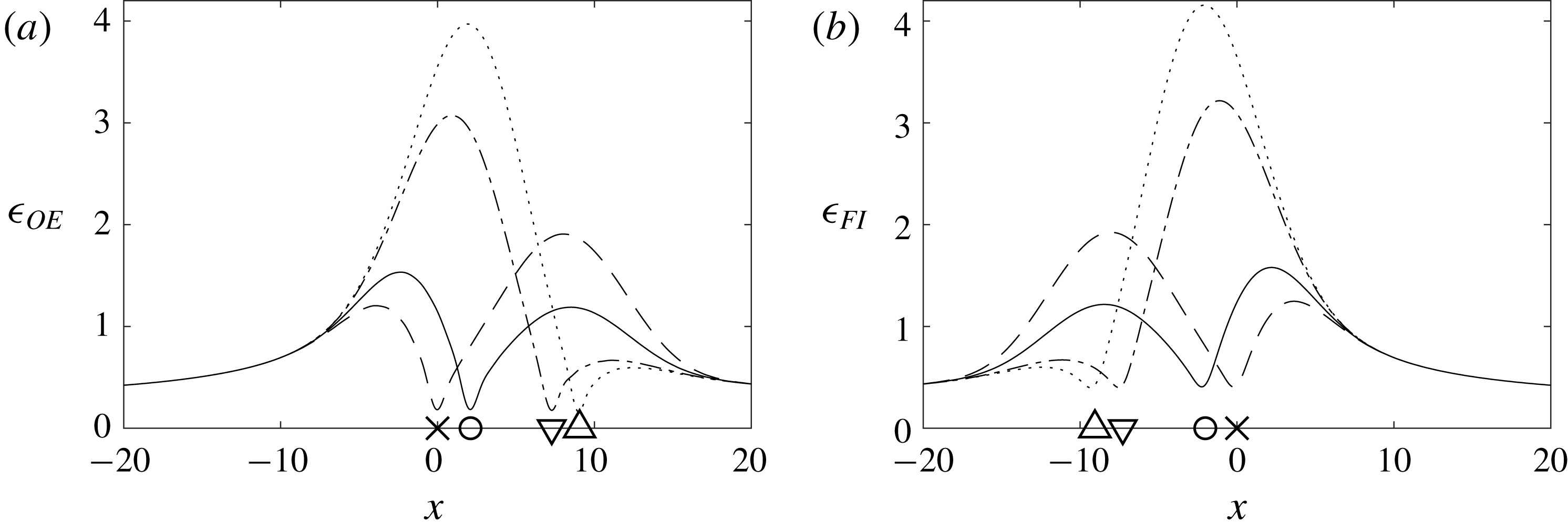
throughout the domain. Figure 5(a) uses the optimal sensor locations from figure 4(c) to calculate
 $\unicode[STIX]{x1D716}_{OE}$
for a range of
 $\unicode[STIX]{x1D707}_{0}$
. As expected, the smallest
 $\unicode[STIX]{x1D716}_{OE}$
occurs at the location of the sensor for all
 $\unicode[STIX]{x1D707}_{0}$
. The most significant contributions to the estimation error are concentrated in two regions: near the centre of the domain and near
 $X_{II}$
.
Similarly, the term
 $\unicode[STIX]{x1D716}_{FI}$
shows the effect of the disturbances on
 $\unicode[STIX]{x1D6FE}_{FI}$
throughout the domain. Figure 5(b) uses the optimal actuator locations from figure 4(c) to calculate
 $\unicode[STIX]{x1D716}_{FI}$
for a range of
 $\unicode[STIX]{x1D707}_{0}$
. The results of figure 5(b) are approximately symmetric to figure 5(a). It is interesting to note that the estimator is the dual of the state feedback controller. Therefore equating the control weight with the sensor noise (
 $v=\unicode[STIX]{x1D6FC}$
, instead of
 $v=10^{-3}$
and
 $\unicode[STIX]{x1D6FC}=1/7$
) would result in
 $x_{s-opt}=-x_{a-opt}$
and an exact symmetry between
 $\unicode[STIX]{x1D716}_{OE}$
and
 $\unicode[STIX]{x1D716}_{FI}$
(Aström & Murray Reference Aström and Murray2010).
(a)
 $\unicode[STIX]{x1D716}_{OE}$
and (b)
 $\unicode[STIX]{x1D716}_{FI}$
as a function of
 $x$
for a range of
 $\unicode[STIX]{x1D707}_{0}$
. Optimal placements from figure 4(c) are used. The locations corresponding to the two peak values of
 $\unicode[STIX]{x1D716}_{OE}$
and
 $\unicode[STIX]{x1D716}_{FI}$
(– –) and the downstream boundary of the unstable domain
 $(\cdots \,)$
are also shown.

4.2 The IOC problem
The results of the OE and FIC problems are relevant for understanding the challenges of sensing and actuating each on their own. However, we cannot use the OE problem for control itself, and in most fluid flows the full-state information needed for FIC is unavailable. Therefore we now combine OE with FIC to form the input–output control (IOC) problem. We will see that similar results to the OE and the FIC problems are obtained.
As in § 4.1, we start with a single value of
 $\unicode[STIX]{x1D707}_{0}=0.41$
with random disturbances applied everywhere in the domain. This time we must consider the sensor
 $(x_{s})$
and actuator
 $(x_{a})$
location together, which adds an extra dimension to the problem. The energy norm
 $\unicode[STIX]{x1D6FE}_{IO}$
is therefore obtained over a range of sensor locations (
 $x_{s}$
) and actuator locations
 $x_{a}$
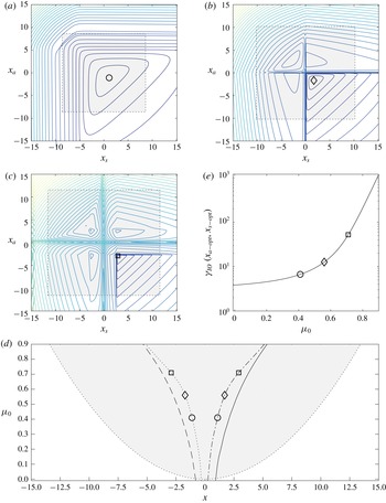
and mapped out on a contour plot in figure 6(a). A minimum of
 $\unicode[STIX]{x1D6FE}_{IO}=6.68$
is achieved for
 $x_{s}=1.09$
and
 $x_{a}=-1.12$
. (These results are consistent with Chen & Rowley (Reference Chen and Rowley2011).) As before, placing the sensor upstream of its optimal location is penalised more severely than placing it downstream. Similarly, placing the actuator downstream of its optimal location is penalised more severely than placing it upstream. These behaviours match those seen for the OE and FIC problems. We repeat the brute force result for
 $\unicode[STIX]{x1D707}_{0}=0.56$
and
 $\unicode[STIX]{x1D707}_{0}=0.71$
in figure 6(b,c), where a minimum of
 $\unicode[STIX]{x1D6FE}_{IO}=12.64$
and
 $\unicode[STIX]{x1D6FE}_{IO}=52.11$
is achieved. Local maxima and rapid changes of
 $\unicode[STIX]{x1D6FE}_{IO}$
are observed at the same locations as for the OE problem and the FIC problem.
Finding the optimum via brute force is computationally expensive – particularly now that the optimisation problem is two-dimensional (with both the sensor and actuator to be chosen simultaneously). Therefore we use the gradient minimisation algorithm of Chen & Rowley (Reference Chen and Rowley2011) to find the optimal sensor
 $x_{s-opt}$
location and the optimal actuator
 $x_{a-opt}$
location – each as a function of
 $\unicode[STIX]{x1D707}_{0}$
.
Figure 6(d) shows that
 $x_{s-opt}$
shifts downstream from
 $0.24$
to
 $5.13$
, while
 $x_{a-opt}$
shifts upstream from
 $-0.33$
to
 $-5.13$
, over the chosen range of
 $-0.01\leqslant \unicode[STIX]{x1D707}_{0}\leqslant 0.9$
. (The sensor and actuator are closer together in IOC than in OE and FIC.) The corresponding optimal positions’
 $\unicode[STIX]{x1D6FE}_{IO}$
are shown in figure 6(e). We can see that
 $\unicode[STIX]{x1D6FE}_{IO}$
increases from
 $3.8$
to
 $1177.5$
, which is significantly larger than for either OE or FIC.
4.3 Discussion
We will now summarise and discuss the main findings.
We first used a brute force approach to generate the energy norm
 $\unicode[STIX]{x1D6FE}$
over a range of sensor and actuator locations. This was done for the OE and FIC problems in figure 4(a,b); and for the IOC problem in figure 6(a–c). Relating the results of figure 4(a,b) to the eigenmodes and adjoint eigenmodes, we see that the energy norm
 $\unicode[STIX]{x1D6FE}_{OE}$
is large at locations where an unstable eigenmode is small (see figure 2
a,c), and that the energy norm
 $\unicode[STIX]{x1D6FE}_{FI}$
is large at locations where an unstable adjoint eigenmode is small (see figure 2
b,d). A similar pattern is seen when comparing figure 6(a–c) with figure 2: that
 $\unicode[STIX]{x1D6FE}_{IO}$
is large at locations where either an unstable eigenmode or an unstable adjoint eigenmode is small. At these locations, the detectability or stabilisability is low, which limits estimation and control (see for example Skogestad & Postlethwaite Reference Skogestad and Postlethwaite2007; Chen & Rowley Reference Chen and Rowley2015).
(a–c) Contours of the IOC norm
 $\unicode[STIX]{x1D6FE}_{IO}$
(Chen & Rowley Reference Chen and Rowley2011), for
 $\unicode[STIX]{x1D707}_{0}$
 $=$
(0.41 (a), 0.56 (b), 0.71 (c)), where the innermost contour is
 $\unicode[STIX]{x1D6FE}_{IO}$
 $=$
(
 $10^{1}$
(a),
 $10^{1.25}$
(b),
 $10^{1.75}$
(c)), and each subsequent contour increments by
 $\times 10^{0.25}$
. (d) The IOC optimal sensor
 $x_{s-opt}$
(– ⋅) and actuator
 $x_{a-opt}$
(:) locations as a function of
 $\unicode[STIX]{x1D707}_{0}$
. The OE and FIC optimal locations are included (——,– –). (a–d) The unstable domain is shaded grey (outer limits (:)); it only exists when
 $\unicode[STIX]{x1D707}_{0}>0$
. (e) The IOC norm
 $\unicode[STIX]{x1D6FE}_{IO}~(x_{s-opt},x_{a-opt})$
as a function of
 $\unicode[STIX]{x1D707}_{0}$
. (a–e) The optimal locations and energy norms for
 $\unicode[STIX]{x1D707}_{0}$
 $=$
(0.41 (○), 0.56 (♢), 0.71 (▫) are indicated.

We are interested in the optimal sensor and actuator locations to achieve the best estimation and control performance possible. The brute force approach is inefficient when searching for the optimal sensor and actuator locations. Instead, we found them by employing the iterative minimisation algorithm of Chen & Rowley (Reference Chen and Rowley2011). At first, we considered the OE and FIC problems in figure 4(c): as the stability decreases (
 $\unicode[STIX]{x1D707}_{0}$
increases) the optimal sensor location
 $x_{s-opt}$
shifts downstream, while the optimal actuator location
 $x_{a-opt}$
shifts upstream. At the same time, the norms
 $\unicode[STIX]{x1D6FE}_{OE}$
and
 $\unicode[STIX]{x1D6FE}_{FI}$
in figure 4(d,e) rise sharply. Thus there is a direct relationship between the stability, optimal location and the energy norm. (The behaviour of
 $x_{a-opt}$
shifting upstream in the FIC problem is also observed by Lauga & Bewley (Reference Lauga and Bewley2003).) The IOC problem shows the same behaviour, although
 $x_{s-opt}$
and
 $x_{a-opt}$
are now closer together (figure 6
d) and
 $\unicode[STIX]{x1D6FE}_{IO}$
is larger (figure 6
e) relative to OE and FIC at a given stability.
An objective of this study is to better understand the optimal sensor and actuator locations we found, with a particular focus on any trade-offs. Therefore, we generated r.m.s. values
 $(\unicode[STIX]{x1D716})$
of
 $\unicode[STIX]{x1D6FE}_{OE}$
and
 $\unicode[STIX]{x1D6FE}_{FI}$
throughout the domain for a set of stabilities in figure 5, placing the sensor and actuator at the respective optimal locations. This provides insight into the relationship between the optimal location, stability, and corresponding energy norm. Two peaks in
 $\unicode[STIX]{x1D716}_{OE}$
can be seen in figure 5(a): one near the centre of the domain and another near
 $X_{II}$
. As
 $\unicode[STIX]{x1D707}_{0}$
increases, the peak near
 $X_{II}$
shifts downstream. The sensor needs to be placed further downstream as well, to ensure that the two peaks are kept as small as possible. Keeping both peaks small is a trade-off in OE, which we further discuss in § 5.1. Two peaks in
 $\unicode[STIX]{x1D716}_{FI}$
can be seen in figure 5(b): one near the centre of the domain and another near
 $X_{I}$
. As
 $\unicode[STIX]{x1D707}_{0}$
increases, the peak at
 $X_{I}$
shifts further upstream. The actuator needs to be placed further upstream as well, to ensure that the two peaks are kept as small as possible. Just as in OE, keeping both peaks small is a trade-off in FIC. The two trade-offs we see in OE and FIC also exist in the IOC problem.
5 Trade-offs in optimal placement
We will now relate the optimal locations found in § 4 to previous studies. This will highlight trade-offs that have to be considered, which were briefly mentioned in § 4.3. Then, we explore some key factors limiting the sensor and actuator placement for effective estimation and control: the eigenmodes, adjoint eigenmodes and time lag. Investigating the effect of time lag is particularly important due to the convective nature of the flow and it will further highlight the effect of the trade-offs that have to be considered. Finally, we discuss the differences seen in the optimal placement results between OE, FIC and IOC.
5.1 Placement prediction
Selected actuator (upstream) and sensor (downstream) placements for
 $\unicode[STIX]{x1D707}_{0}=0.41$
based on previous literature:
 $X_{I}$
and
 $X_{II}$
(▵),
 $\unicode[STIX]{x1D713}_{0}$
and
 $\unicode[STIX]{x1D719}_{0}$
(▿),
 $\unicode[STIX]{x1D701}_{0}$
(
 $\times$
) and
 $H_{2}$
-optimal (○). The normalised most unstable eigenmode
 $\unicode[STIX]{x1D719}_{0}$
(——), the normalised most unstable adjoint eigenmode
 $\unicode[STIX]{x1D713}_{0}$
(– –) and their corresponding wavemaker region
 $\unicode[STIX]{x1D701}_{0}$
(– ⋅) are included. The unstable domain, with upstream
 $(X_{I})$
and downstream (
 $X_{II}$
) branches, is shown.

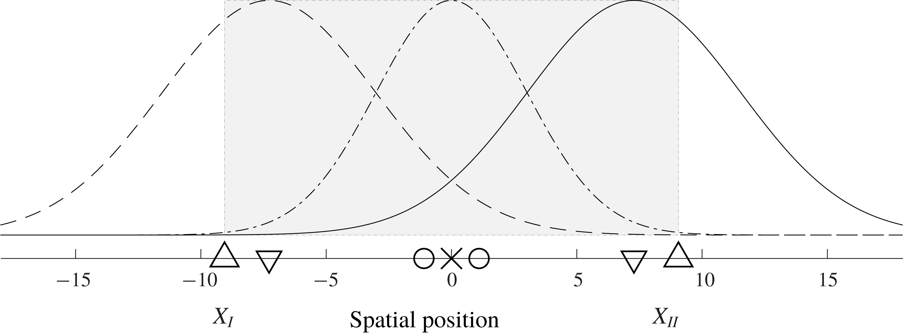
We now consider the optimal placements for OE and FIC at
 $\unicode[STIX]{x1D707}_{0}=0.41$
along with three placements based on previous literature: the most unstable eigenmode
 $(\unicode[STIX]{x1D719}_{0})$
and adjoint eigenmode
 $(\unicode[STIX]{x1D713}_{0})$
, the wavemaker region (
 $\unicode[STIX]{x1D701}_{0}$
) and the downstream (
 $X_{II}$
) and upstream (
 $X_{I}$
) branches of the unstable domain. These are shown in figure 7 (see Åkervik et al.
Reference Åkervik, Hœpffner, Ehrenstein and Henningson2007; Giannetti & Luchini Reference Giannetti and Luchini2007; Bagheri et al.
Reference Bagheri, Henningson, Hœpffner and Schmid2009; Chen & Rowley Reference Chen and Rowley2011, Reference Chen and Rowley2015). We see in figure 4(a,b) that the wavemaker region (
 $\unicode[STIX]{x1D701}_{0}$
) provides the best prediction of the optimal placement. Still, the placement based on the wavemaker region does not perform as well as the optimal placement. To understand why, we will now study the
 $\unicode[STIX]{x1D716}_{OE}$
and
 $\unicode[STIX]{x1D716}_{FI}$
values for each of the four placement, which we display in figure 8.
(a)
 $\unicode[STIX]{x1D716}_{OE}$
, and (b)
 $\unicode[STIX]{x1D716}_{FI}$
, as a function of
 $x$
, for the four placements based on
 $X_{II}$
and
 $X_{I}$
(:),
 $\unicode[STIX]{x1D719}_{0}$
and
 $\unicode[STIX]{x1D713}_{0}$
(⋅ –),
 $\unicode[STIX]{x1D701}_{0}$
(– –) and
 $H_{2}$
-optimal (——). The respective norms are
 $\unicode[STIX]{x1D6FE}_{OE}=(11.0,8.7,6.6,5.7)$
and
 $\unicode[STIX]{x1D6FE}_{FI}=(11.5,9.1,6.7,5.9)$
.

In figure 8(a), for every placement case there exist two peaks of
 $\unicode[STIX]{x1D716}_{OE}$
: one upstream of the sensor and one downstream of the sensor. The downstream peak for the sensor placement at
 $X_{II}$
is the smallest. However, the trade-off is that the upstream peak is the largest. The converse is true for wavemaker-based placement: the downstream peak is the largest, while the upstream peak is the smallest. The best trade-off is given by the
 $H_{2}$
-optimal placement. The optimal location provides the best compromise between keeping the upstream peak small and keeping the downstream peak small, which agrees with findings of Colburn (Reference Colburn2011). At the optimal location,
 $59\,\%$
of the energy contributed to
 $\unicode[STIX]{x1D6FE}_{OE}$
is from upstream of the sensor, and the remainder from downstream.
We can draw similar observations for FIC in 8(b): the optimal location provides the best compromise between keeping the upstream and downstream peak of
 $\unicode[STIX]{x1D716}_{FI}$
small.
5.2 The effect of eigenmodes and adjoint eigenmodes
We saw in § 5.1 that the eigenmodes and adjoint eigenmodes fail to predict the optimal placement for estimation and control. They fail because of the non-normal, convective nature of the CGLE (e.g. Bagheri et al.
Reference Bagheri, Henningson, Hœpffner and Schmid2009; Schmid & Henningson Reference Schmid and Henningson2012). Yet, they do show locations where a particular mode can be measured and actuated effectively. For example, both the second eigenmode
 $(\unicode[STIX]{x1D719}_{1})$
and adjoint eigenmode
 $(\unicode[STIX]{x1D713}_{1})$
are zero at the domain’s centre (figure 2). Therefore placement at the domain’s centre
 $(x_{s}=x_{a}=0)$
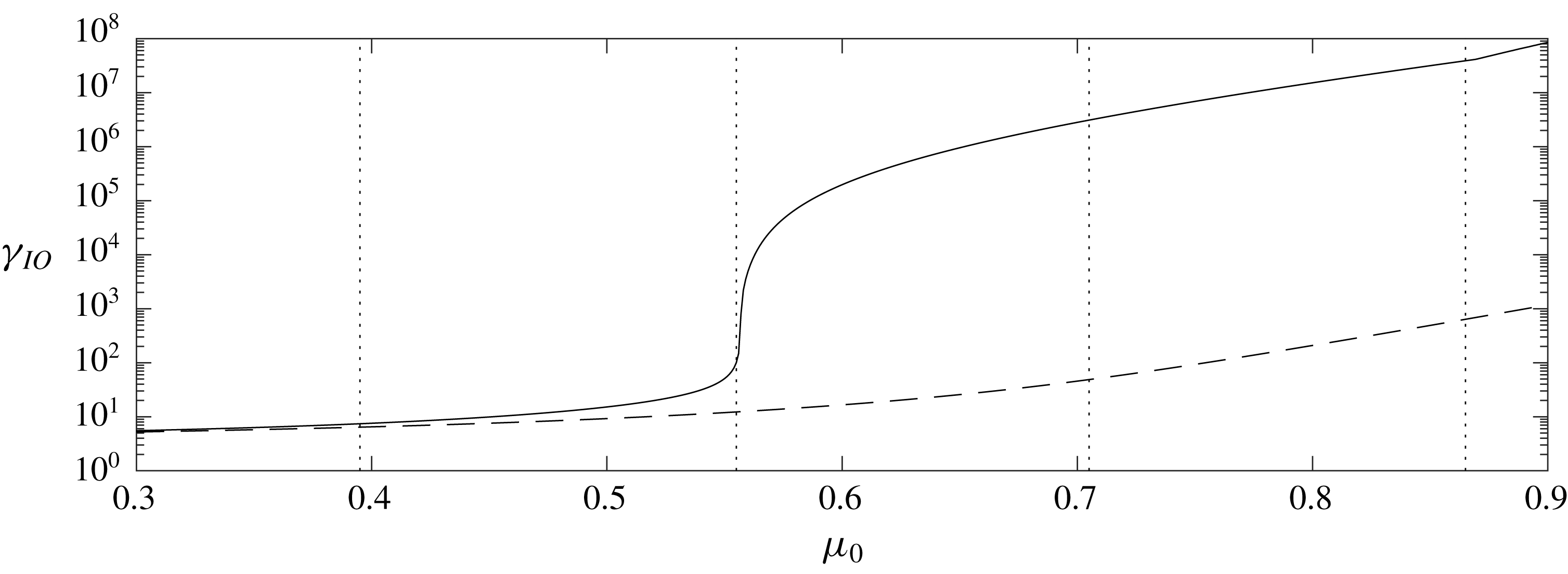
results in poor performance when the second mode is unstable (see figures 4(a,b) and 6(a–c)). We illustrate this in figure 9, where we plot
 $\unicode[STIX]{x1D6FE}_{IO}$
as a function of
 $\unicode[STIX]{x1D707}_{0}$
for
 $x_{s}=x_{a}=0$
and compare it to
 $\unicode[STIX]{x1D6FE}_{IO}$
for the optimal placement. The placement at
 $x_{s}=x_{a}=0$
performs similarly to the optimal placement as long as only one mode is unstable. There is a sharp increase in
 $\unicode[STIX]{x1D6FE}_{IO}$
when the second mode becomes unstable. Changing
 $\unicode[STIX]{x1D707}_{0}$
from
 $0.55$
to
 $0.56$
increases
 $\unicode[STIX]{x1D6FE}_{IO}$
from
 $50.8$
to
 $4949.1$
. (Similar changes are observed for OE and FIC.) One may ask why control does not become impossible in this case? The answer is that both the sensor and actuator have Gaussian profiles in space (see (B 2a
) and (B 2b
)), and therefore sensing and actuation occur not just at
 $x=0$
, but also in its vicinity. This somewhat severe example helps to highlight the importance of the eigenmodes and adjoint eigenmodes. Placement without their consideration leads to poor performance.
(a) Variation of
 $\unicode[STIX]{x1D6FE}_{IO}$
as a function of
 $\unicode[STIX]{x1D707}_{0}$
when
 $(x_{s},x_{a})$
is:
 $(0,0)$
(——) and
 $(x_{s-opt},x_{a-opt})$
(– –). The threshold of instability for the first four modes is indicated by (
 $\cdots \!$
) from left to right.

5.3 The effect of time delay
Chen & Rowley (Reference Chen and Rowley2011, Reference Chen and Rowley2015) pointed out the detrimental effect of excessive time lag, which causes the wavemaker region to be the best predictor of the optimal placement in § 5.1. To better understand and quantify the time-lag effect we now introduce an artificial delay
 $\unicode[STIX]{x1D70F}$
to either the sensor signal
 $\boldsymbol{y}$
(OE and IOC) or the actuator signal
 $\boldsymbol{u}$
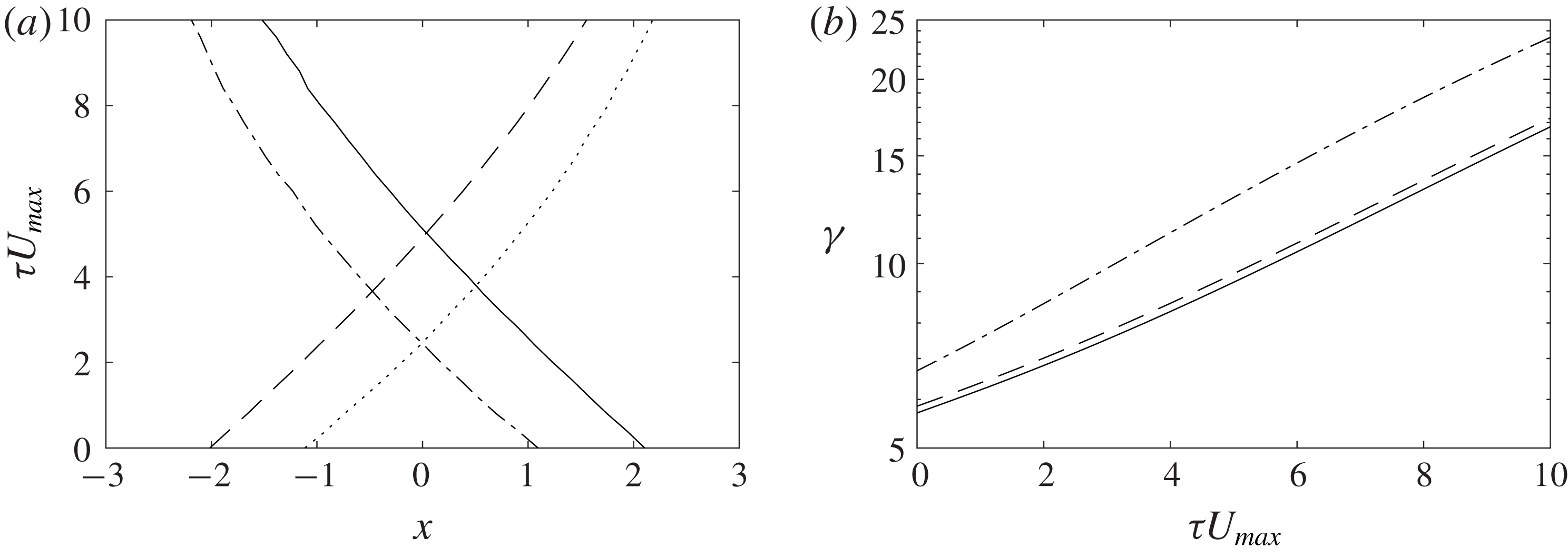
(FIC). The delay is introduced into the signals via a Padé approximation of order ten. Figure 10 shows the optimal sensor locations, the optimal actuator locations and the corresponding energy norms as a function of
 $\unicode[STIX]{x1D70F}$
at
 $\unicode[STIX]{x1D707}_{0}=0.41$
. The delay
 $\unicode[STIX]{x1D70F}$
is normalised with
 $U_{max}$
(the overall group velocity of the perturbations, see § 2.1) to represent distance travelled by perturbations during the delay. With increasing
 $\unicode[STIX]{x1D70F}$
the optimal sensor locations shift upstream, and the optimal actuator locations downstream, while the amount of spatial shift relative to
 $U_{max}\unicode[STIX]{x1D70F}$
is similar. At the same time, the energy norms increase by
 $193\,\%$
for OE,
 $196\,\%$
for FI and
 $250\,\%$
for IO over the given time-lag range.
The optimal sensor location moves further upstream to compensate for the artificial time lag in the measurement signal. The actuator moves further downstream to compensate for the delay in the feedback loop. These shifted optimal locations provide the best compromise between keeping the upstream and downstream peaks of the corresponding
 $\unicode[STIX]{x1D716}$
small (as discussed in § 5.1) when subject to an artificial time lag. For a particular delay, the optimal sensor and actuator locations coincide with the peak of the wavemaker region.
(a) The optimal sensor location (OE:
 $x_{s-opt}$
(——), IO:
 $x_{s-opt}$
(– ⋅)) and the optimal actuator location (FI:
 $x_{a-opt}$
(– –), IO:
 $x_{a-opt}$
(
 $\cdots \,$
)) as a function of
 $\unicode[STIX]{x1D70F}U_{max}$
(delay scaled by the group velocity); (b) the corresponding,
 $\unicode[STIX]{x1D6FE}_{OE}$
(——),
 $\unicode[STIX]{x1D6FE}_{FI}$
(– –), and
 $\unicode[STIX]{x1D6FE}_{IO}$
(– ⋅).

5.4 The difference between the optimal placements of OE, FIC and IOC
The separation principle of estimation and control states that when combining the independently designed optimal estimator, with the full information controller, the resulting input–output controller is still optimal. However, figure 6(d) shows that the optimal sensor and actuator locations for OE and FIC do not match the optimal sensor and actuator locations for IOC. This mismatch is because the separation principle only affects the estimator and controller design problem, but not the placement problem itself. It is essential to estimate perturbations which improve the control decision, hence the optimal sensor location for the IOC problem is closer to the centre of the domain than for OE problem. Similarly, it is essential to control perturbations which reduce the estimation error, and therefore the optimal actuator location for the IOC problem is closer to the centre of the domain than for the FIC problem.
6 Conclusion
Previous feedback flow control studies have placed sensors and actuators based on physical characteristics, such as eigenmodes. These physical characteristics are useful for understanding the limitations of effective estimation and control, but by themselves, they do not provide the whole picture. Instead, one has to search for the optimal locations iteratively, as done by Chen & Rowley (Reference Chen and Rowley2011). We have studied the single sensor and single actuator placement problem in the complex Ginzburg–Landau equation over a range of stabilities. Specifically, we investigated any trade-offs present when searching for the optimal sensor and actuator locations.
The current study has made plain conflicting trade-offs. The sensor needs to be placed far enough downstream to estimate the end of the unstable domain, where perturbations are most energetic; and far enough upstream to estimate the remaining less energetic perturbations. The actuator needs to be placed far enough upstream to control the beginning of the unstable domain, where disturbances have the greatest potential for amplification; and far enough downstream to control the remaining disturbances with less potential for amplification. When considering the sensor and actuator placement problem together, both trade-offs will also interact with each other, resulting in a slight shift of the optimal locations. Despite these relatively small differences between the optimal locations, we have observed a consistent trend in which the optimal sensor location moves downstream, and the optimal actuator location moves upstream with decreasing stability; conversely, these trade-offs cause a consistent trend in which the sensor moves upstream, and the actuator moves downstream with increasing time lag in measurement and actuation. It would be interesting to see if these trends are also observed in other convection-dominated spatially developing flows, such as jets and wakes. A future study could consider optimal sensor and actuator placement for control of vortex shedding over a range of Reynolds numbers.
Acknowledgement
The authors are grateful for the financial support of the Australian Research Council.
Appendix A. Spectral discretisation of the continuous equation
For this study, we considered three discretisation methods: Hermite collocation on an infinite domain (Weideman & Reddy Reference Weideman and Reddy2000), Chebyshev collocation on a finite domain (Trefethen Reference Trefethen2000) and Chebyshev collocation on an infinite domain (Schmid & Henningson Reference Schmid and Henningson2012). Convergence and scaling studies showed convergence for all three methods. We selected the finite Chebyshev collocation methods for this study because it requires the lowest order for convergence.
We employ Chebyshev collocation of order
 $N_{c}=N+1=151$
, scale the Chebyshev points by
 $L=25$
and enforce boundary conditions to obtain at a system with
 $N$
grid points, i.e.
 $\boldsymbol{x}=[x_{1},x_{2},\ldots x_{i},\ldots x_{N}]^{\text{T}}$
, extending from
 $-L<x_{i}<L$
. Discrete integration is implemented using the Clenshaw–Curtis quadrature, which provides weights
 $w_{i}$
at each Chebyshev point and is used to form the integration matrix:
 $\unicode[STIX]{x1D648}=\text{diag}(L[w_{1},w_{2},\ldots w_{i}\ldots ,w_{N}])$
. The discrete representation is then of the form:
 $$\begin{eqnarray}\displaystyle \dot{\boldsymbol{q}}(t)=(-\unicode[STIX]{x1D708}\unicode[STIX]{x1D63F}+\unicode[STIX]{x1D705}\unicode[STIX]{x1D71F}+\text{diag}(\unicode[STIX]{x1D741}))\boldsymbol{q}(t)+\unicode[STIX]{x1D63D}_{d}\boldsymbol{d}(t)=\unicode[STIX]{x1D63C}\boldsymbol{q}(t)+\unicode[STIX]{x1D63D}_{d}\boldsymbol{d}(t), & & \displaystyle\end{eqnarray}$$
where
 $\unicode[STIX]{x1D63F}$
and
 $\unicode[STIX]{x1D71F}$
are the first- and second-order Chebyshev differentiation matrices with suitable boundary conditions and
 $\unicode[STIX]{x1D63C}$
is the discrete complex Ginzburg–Landau operator. At each grid point
 $i$
, we apply random forcing which is white in space and time with a covariance
 $\text{E}(d_{i}\bar{d_{i}})=1$
, where
 $\text{E}$
the expected value. Setting
 $\unicode[STIX]{x1D63D}_{d}=\unicode[STIX]{x1D648}^{-(1/2)}$
ensures that the disturbances are grid size independent.
Appendix B. The systems for estimation and control
This section will supplement § 3 by describing the OE, FIC and IOC problems (Kim & Bewley (Reference Kim and Bewley2007), Skogestad & Postlethwaite (Reference Skogestad and Postlethwaite2007), Aström & Murray (Reference Aström and Murray2010)). The OE, FIC and IOC three problems can be cast into the same general form:
 $$\begin{eqnarray}\displaystyle \unicode[STIX]{x1D64B}:\left[\!\begin{array}{@{}c@{}}\dot{\boldsymbol{q}}(t)\\ \boldsymbol{z}(t)\\ \boldsymbol{y}(t)\end{array}\!\right]=\left[\!\begin{array}{@{}ccc@{}}\unicode[STIX]{x1D63C} & \unicode[STIX]{x1D63D}_{w} & \unicode[STIX]{x1D63D}_{u}\\ \unicode[STIX]{x1D63E}_{z} & \mathbf{0} & \unicode[STIX]{x1D63F}_{u}\\ \unicode[STIX]{x1D63E}_{y} & \unicode[STIX]{x1D63F}_{w} & \mathbf{0}\end{array}\!\right]\left[\!\begin{array}{@{}c@{}}\boldsymbol{q}(t)\\ \boldsymbol{w}(t)\\ \boldsymbol{u}(t)\end{array}\!\right]. & & \displaystyle\end{eqnarray}$$
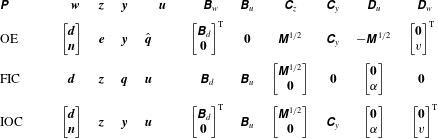
The inputs, outputs and matrices for the OE, FIC and IOC problems.
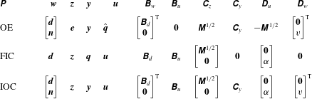
Table 2 lists the inputs, outputs and system matrices for the OE, FI and IOC problems. These signals and matrices were already introduced in (3.1) and § 3. A single sensor is placed at
 $x_{s}$
and a single actuator is placed at
 $x_{a}$
. We use the expressions from the previous literature (Bagheri et al.
Reference Bagheri, Henningson, Hœpffner and Schmid2009; Chen & Rowley Reference Chen and Rowley2011) to define the spatial extent of the sensor
 $\unicode[STIX]{x1D63E}_{y}$
and actuator
 $\unicode[STIX]{x1D63D}_{u}$
as Gaussian functions:
 $$\begin{eqnarray}\displaystyle & \displaystyle \unicode[STIX]{x1D63E}_{y}=\exp \left\{-\left(\frac{\boldsymbol{x}-x_{s}}{\sqrt{2}\unicode[STIX]{x1D70E}}\right)^{2}\right\}^{\text{T}}\unicode[STIX]{x1D648}, & \displaystyle\end{eqnarray}$$
 $$\begin{eqnarray}\displaystyle & \displaystyle \unicode[STIX]{x1D63D}_{u}=\exp \left\{-\left(\frac{\boldsymbol{x}-x_{a}}{\sqrt{2}\unicode[STIX]{x1D70E}}\right)^{2}\right\}, & \displaystyle\end{eqnarray}$$
 $\unicode[STIX]{x1D70E}=0.4$
is the variance of the Gaussian function.
Appendix C. Optimal placement
Following the work of Chen & Rowley (Reference Chen and Rowley2011, Reference Chen and Rowley2014, Reference Chen and Rowley2015) we use a location perturbation technique to calculate changes of
 $\unicode[STIX]{x1D6FE}$
with respect to the sensor and actuator locations. These derivatives can be employed with a gradient minimisation technique to solve for the optimal
 $\unicode[STIX]{x1D6FE}$
. Examples of gradient minimisation techniques include the Polak–Ribiere conjugate gradient method or the Broyden–Fletcher–Goldfarb–Shannon quasi-Newton algorithm.
We obtained the IOC problem’s derivatives with respect to the sensor and actuator location from Chen & Rowley (Reference Chen and Rowley2011). To obtain the OE problem’s derivative with respect to the sensor location and the FIC problem’s derivative with respect to the actuator location we adapted the work of Chen & Rowley (Reference Chen and Rowley2011):
 $$\begin{eqnarray}\displaystyle \frac{\unicode[STIX]{x1D6FF}(\unicode[STIX]{x1D6FE}_{OE}^{2})}{\unicode[STIX]{x1D6FF}x_{s}}=\frac{\text{tr}(\unicode[STIX]{x1D63E}_{z}\unicode[STIX]{x1D739}\unicode[STIX]{x1D654}\unicode[STIX]{x1D63E}_{z}^{\ast })}{\unicode[STIX]{x1D6FF}x_{s}},\quad \frac{\unicode[STIX]{x1D6FF}(\unicode[STIX]{x1D6FE}_{FI}^{2})}{\unicode[STIX]{x1D6FF}x_{a}}=\frac{\text{tr}(\unicode[STIX]{x1D63D}_{w}^{\ast }\unicode[STIX]{x1D739}\unicode[STIX]{x1D653}\unicode[STIX]{x1D63D}_{w})}{\unicode[STIX]{x1D6FF}x_{a}}. & & \displaystyle\end{eqnarray}$$
Appendix D. The root mean square of the norm
The root mean square (r.m.s.) value
 $\unicode[STIX]{x1D716}(x)$
is defined to have the following property:
 $$\begin{eqnarray}\displaystyle \unicode[STIX]{x1D6FE}^{2}=\int _{-\infty }^{\infty }\unicode[STIX]{x1D716}^{2}(x)\,\text{d}x=\text{sum}(\text{diag}(\unicode[STIX]{x1D71E}))=\text{sum}(\unicode[STIX]{x1D648}\unicode[STIX]{x1D750}\odot \unicode[STIX]{x1D750}), & & \displaystyle\end{eqnarray}$$
where
 $\unicode[STIX]{x1D71E}$
describes the covariance matrix (Bagheri et al.
Reference Bagheri, Henningson, Hœpffner and Schmid2009),
 $\unicode[STIX]{x1D750}$
describes the discrete r.m.s. values and
 $\odot$
the Hadamard product. We can solve for
 $\unicode[STIX]{x1D750}$
by rearranging (D 1):
 $$\begin{eqnarray}\displaystyle \unicode[STIX]{x1D750}=(\unicode[STIX]{x1D648}^{-1}\,\text{diag}(\unicode[STIX]{x1D71E}))^{\odot (1/2)}, & & \displaystyle\end{eqnarray}$$
where
 $()^{\odot }$
is the Hadamard power.