1. Introduction
Alan Author has just made an important discovery. From his calculations it follows that recent evidence e supports the conjunction of two popular hypotheses,  $h_{1}$ and
 $h_{2}$. With great gusto he sets himself to the writing of a research proposal in which he explains his idea and asks for time and money to work out all its far-reaching consequences. Alan Author's proposal is sent to Rachel Reviewer, who—to his dismay—writes a devastating report. Ms. Reviewer first recalls what is common knowledge within the scientific community, namely that e strongly disconfirms not only
 $h_{1}$, but also
 $h_{2}$ as well. Then she intimates that Alan Author is clearly not familiar with the relevant literature; for if he were, he would have realized that any calculation that results in confirming the conjunction of two disconfirmed hypotheses must contain a mistake. At any rate, he should never have launched this preposterous idea, which will make him the laughing stock of his peers.
Is Reviewer right? Did Author indeed make a blunder by assuming that e might confirm a conjunction of hypotheses,  $h_{1}\wedge h_{2}$, given that the same e disconfirms
 $h_{1}$ and
 $h_{2}$ separately? In this article we will argue that Author may not have been mistaken. If c is some generic confirmation function, then it can happen that
 $c( h_{1}\wedge h_{2},\, e) $ is greater than zero, indicating confirmation of the conjunction of the hypotheses, while
 $c( h_{1},\, e) $ and
 $c( h_{2},\, e) $ are both less than zero, indicating disconfirmation of each hypothesis separately. Friend Author might have written a defensible proposal after all.
Our article can be seen as a reinforcement of recent claims made by Crupi, Fitelson, and Tentori (Reference Crupi, Fitelson and Tentori2008). In this very stimulating paper, the authors (henceforth CFT) introduce the two inequalitiesFootnote 1

Next they convincingly argue that (1) is a sufficient condition for

In other words, if e disconfirms  $h_{1}$, but confirms
 $h_{2}$ when
 $h_{1}$ is true, then e gives more confirmation to
 $h_{1}\wedge h_{2}$ than to
 $h_{1}$ alone—although it confirms
 $h_{2}$ alone even more:
 $c( h_{2},\, e) > c( h_{1}\wedge h_{2},\, e) $.
The fact that e can give more confirmation to  $h_{1}\wedge h_{2}$ than to one of its conjuncts is of course intriguing, since the corresponding claim for conditional probabilities is false. Under no condition whatsoever can it be true that

Indeed, (3) instantiates the notorious conjunction fallacy. Ever since its description by Tversky and Kahneman (Reference Tversky and Kahneman1983), various explanations of the conjunction fallacy have been put forward. Fisk (Reference Fisk and Pohl2004) discusses no less than nine different explanations (ranging from an appeal to linguistic misunderstandings to the idea that people resort to some form of averaging process in deriving conjunctive judgments) only to conclude that none of them is convincing. As to Tversky and Kahneman's own account—based as it is on their earlier ideas about representativeness (Kahneman and Tversky Reference Kahneman and Tversky1972, Reference Kahneman and Tversky1973)—Fisk reports that it failed several empirical tests (Reference Fisk and Pohl2004, 28). His overall judgment is that “an adequate account of the fallacy remains elusive” (Reference Fisk and Pohl2004, 40).
As CFT see it, most of the explanations endorse the following inference: first, a formally defined attribute is identified—which, in certain conditions, would rank  $h_{1}\wedge h_{2}$ over one of its conjuncts—then the conclusion is immediately drawn that this attribute explains the fallacy. But, as CFT note, “pending an independent argument to the effect that in standard probabilistic (and betting) conjunction tasks participants are rationally justified in evaluating something else other than probabilities
 $P( h_{1}\vert e) $ and
 $P( h_{1}\wedge h_{2}\vert e) $, we see this inference as spurious” (Crupi et al. Reference Crupi, Fitelson and Tentori2008, 191).
Following a suggestion by Sides et al. (Reference Sides, Osherson, Bonini and Viale2002), CFT offer a different account. They surmise that the conjunction fallacy might arise from a confusion between (2) and (3). We find this idea plausible and promising, all the more so because it appears to have solid empirical support (Tentori et al. Reference Tentori, Crupi, Bonini and Osherson2007). However, we also believe that the scope of this idea can be significantly expanded. For if we replace CFT's condition (1) by another sufficient condition, then we are able to obtain a much stronger result. In this article we will argue that if we take as condition

then it can be shown that

There are two senses in which (5) is more general, and cuts deeper than CFT's result (2). First, (5) implies that there is a situation in which the conjunction  $h_{1}\wedge h_{2}$ is more, or equally, confirmed than either of the conjuncts—whereas (2) implies that only one of the conjuncts receives less confirmation than the conjunction. Second, (5) is also applicable when both
 $h_{1}$ and
 $h_{2}$ are confirmed—whereas (2) requires that one of the hypotheses must be disconfirmed. Hence, CFT's explanatory net can in fact be cast much more widely than they do, since there appear to be more ways in which the occurrence of a conjunction fallacy might actually be guided by a sound assessment of a confirmation relation. Of course, this is still open to experiment—here we are simply formulating hypotheses that can be tested empirically.
Condition (4) states that, if e is the case, then either both  $h_{1}$ and
 $h_{2}$ are true, or neither is:
 $P( h_{1}\leftrightarrow h_{2}\vert e) =1$. This is sufficient for (5), as we will prove in Section 2 and in Appendix A. However, it is by no means necessary, as will become clear from Section 4 and Appendix B, cf. (13). There we describe a sufficient condition under which
 $c( h_{1}\wedge h_{2},\, e) $ is positive, but both
 $c( h_{1},\, e) $ and
 $c( h_{2},\, e) $ are negative:

Note that (6) describes the case in which Alan Author would be vindicated after all. As we will explain later, the sufficient condition for (6) is more detailed than (4). In fact, as we will see from (13), it consists of a relaxed version of (4)—in the sense that small, nonzero values of the two conditional probabilities are tolerated—plus some extra constraints. Since (6) implies (5), but not the other way around, the sufficient condition for (6) also suffices for (5). In this sense, a relaxed version of (4), together with some constraints that we will spell out later, would still be enough to deduce (5).
2. Robust Confirmation
CFT justly emphasize that their analysis is robust: it holds for various specifications of the generic function  $c( h,e) $, that is, for various measures of confirmation (cf. Fitelson Reference Fitelson1999). In general, a confirmation function
 $c( h,e) $ is a measure of the increase in probability that a hypothesis acquires when some evidence for its veracity is added. It is an increasing function of the conditional probability of the hypothesis (at constant unconditional probability), and a decreasing function of the unconditional probability (at constant conditional probability). CFT list six prevailing confirmation measures that satisfy these necessary conditions, and they prove that their conclusions follow for any of them. We will demonstrate that our argument also goes through robustly in this sense. Indeed, we will add three more measures of confirmation to those listed by CFT, making nine measures in all. The nine measures in question are the following—where, as usual,
 $P( h\vert e) $ denotes a conditional, and
 $P( h) $ an unconditional probability:


The first six of these measures have been discussed by CFT. Measure C is attributed to Carnap (Reference Carnap1950), D to Carnap (Reference Carnap1950) and Eells (Reference Eells1982), S to Christensen (Reference Christensen1999) and Joyce (Reference Joyce1999), Z to Crupi, Tentori and Gonzalez (Reference Crupi, Tentori and Gonzalez2007), R to Keynes (Reference Keynes1921) and Milne (Reference Milne1996), and L to Good (Reference Good1950) and Fitelson (Reference Fitelson2001).
The three extra measures that we have added are N, K, and F. Measures N and K have been taken from Tentori et al. (Reference Tentori, Crupi, Bonini and Osherson2007), who attribute them respectively to Nozick (Reference Nozick1981), and Kemeny and Oppenheim (Reference Kemeny and Oppenheim1952). Note that  $N( h,\, e) =S( e,\, h) $ and
 $K( h,\, e) =F( e,\, h) $. F is inspired by a measure introduced by Fitelson (Reference Fitelson2003). The latter is in fact a measure of coherence rather than of confirmation. However, it is well known that there are close conceptual connections between coherence and confirmation, and confirmation measures are sometimes used to indicate coherence (cf. Douven and Meijs Reference Douven and Meijs2006). For example, Carnap's confirmation measure D, to which Carnap himself gives special attention in (Carnap Reference Carnap1962), is the favorite measure of coherence of Douven and Meijs (Reference Douven2007). Further, the exponent of the confirmation measure R of Keynes and Milne,
 $\mathrm{exp}\,R( h,\, e) $, is equal to a coherence measure of Shogenji (Reference Shogenji1999).
CFT succeed in showing that their inference from (1) to (2) remains valid under any of their six measures of confirmation. Similarly, we can prove that our inference from (4) to (5) remains valid as one passes from one of the nine specifications of  $c( h,\, e) $ to another. Take for example the case in which
 $c( h,\, e) $ is specified as the Carnap-Eells measure
 $D( h,\, e) $. We prove in Appendix A that, if our condition (4) is fulfilled, then

and similarly with  $h_{1}$ and
 $h_{2}$ interchanged. Clearly, if (7) holds, then
 $D( h_{1}\wedge h_{2},\, e) \geq D( h_{1},\, e) $, which is the first half of our conclusion (5), with D substituted for c. An analogous argument applies to
 $h_{2}$, and this will give us the second half of (5).Footnote 2
Similarly, but with more effort, it can be shown that all the remaining specifications of c in terms of  $C,\, S,\, Z,\, R,\, L,\, N,\, K$, and F will do the trick: they lead to quotients of products of probabilities that are necessarily nonnegative. In this manner we will have robustly deduced the two inequalities of (5) from (4). Full details are given in Appendix A, where in passing we also explain under which additional conditions (5) is deducible with > in place of ≥.Footnote 3
As said above, the condition (4) is sufficient, but by no means necessary, for (5)—for it still follows robustly if the probabilities in (4) are small but not zero, and if some extra constraints are in force. In Section 4 and in Appendix B, we will formulate upper bounds for  $P( h_{1}\wedge \neg h_{2}\vert e) $ and
 $P( \neg h_{1}\wedge h_{2}\vert e) $—as well as extra constraints such that (5) still holds robustly, that is, under any of the nine confirmation measures in our list. But first, in Section 3, we will illustrate the validity of our inference from (4) to (5) with some examples. The purpose of this exercise is to make the inference intuitively reasonable and to explain its connection to a (particular type of) conjunction fallacy.
3. Conjunction Fallacies
Suppose a roulette wheel bearing the numbers 1 to 10 is spun in secrecy and the number that comes up is recorded by the game master. Consider two gamblers who entertain different hypotheses about what the number is. Hypothesis  $h_{1}$ is that the number is 2 through 5, or perhaps 9—whereas
 $h_{2}$ is that it is 5 through 8, or perhaps 3. We conclude that

Suppose next that the game master provides the clue that the number is prime. This can be treated as incoming evidence  $e=\{ 2,\, 3,\, 5,\, 7\} $, with
 $h_{1}=\{ 2,\, 3,\, 4,\, 5,\, 9\} $ and
 $h_{2}=\{ 3,\, 5,\, 6,\, 7,\, 8\} $. Since e contains four primes, whereas
 $h_{1}$ and
 $h_{2}$ contain only three primes apiece, we find for the conditional probabilities

Let us now work out this example in terms of the Carnap-Eells measure D, keeping in mind that similar results apply to any of the other nine measures. Since by definition  $D( h,\, e) =P( h\vert e) -P( h) $, it is the case that

and similarly  $D( h_{2},\, e) =1/ 4$. However
 $h_{1}\wedge h_{2}=\{ 3,\, 5\} $, so
 $P( h_{1}\wedge h_{2}\vert e) =2/ 4=1/ 2$, which is strictly less than
 $P( h_{1}\vert e) $ or
 $P( h_{2}\vert e) $; but
 $P( h_{1}\wedge h_{2}) =2/ 10=1/ 5$, which is strictly less than
 $P( h_{1}) $ or
 $P( h_{2}) $.
The Carnap degree of confirmation of  $h_{1}\wedge h_{2}$ is

which is strictly larger than the degrees of confirmation of  $h_{1}$ or
 $h_{2}$. So

and this is our result (5), with D substituted for c, and ≥ replaced by >.
It is intuitively clear why  $e=\{ 2,\, 3,\, 5,\, 7\} $ should confirm
 $h_{1}\wedge h_{2}=\{ 3,\, 5\} $ more than
 $h_{1}=\{ 2,\, 3,\, 4,\, 5,\, 9\} $ or
 $h_{2}=\{ 3,\, 5,\, 6,\, 7,\, 8\} $, since
 $h_{1}\wedge h_{2}$ contains only primes, whereas
 $h_{1}$ and
 $h_{2}$ are each ‘diluted’ by nonprimes. However, by the same token it also seems clear how this example can trigger the commission of a conjunction fallacy. Imagine that subjects are given the following information.
A game master spins a roulette wheel. He records the number, but does not tell anybody what it is. The only thing he makes known is that the number is prime (e). Suppose that now the question is posed, What do you think is more probable? That the number recorded by the game master is 2 through 5, or perhaps 9 ( $h_{1}$)? That it is 5 through 8, or perhaps 3 (
 $h_{2}$)? Or that it is 3 or 5 (
 $h_{1}\wedge h_{2}$)? It is quite likely that many people would choose the last option, thereby committing a conjunction fallacy (although they would have been right had the question been about confirmation rather than probability).
Here is a different example. Imagine that you have a little nephew of whom you are very fond. One day you receive an e-mail from his mother, telling you that the child is suffering a severe bout of measles (e). You immediately decide to visit the boy, bringing him some of the jigsaw puzzles that you know he likes so much. What do you think is more probable to find upon your arrival? That the child has a fever ( $h_{1}$), that he has red spots all over his body (
 $h_{2}$), or that he has a fever and red spots (
 $h_{1}\wedge h_{2}$)? Again we expect that many people will opt for the third possibility. Although this answer is fallacious, the nephew story does instantiate our inference from (4) to (5). Under the assumption that measles always comes with fever and red spots—so that (4) is satisfied—our story makes it true thatFootnote 4

It should be noted that the conjunction fallacies committed in the two examples above differ from those discussed by CFT, who focus exclusively on conjunction fallacies of the Linda-type, as described by Tversky and Kahneman (Reference Tversky and Kahneman1983): when hearing about a person named Linda, who is 31 years old, single, bright and outspoken, concerned about discrimination and social justice, involved in antinuclear demonstrations (e), most people find ‘Linda is a bank teller and is active in the feminist movement’ ( $h_{1}\wedge h_{2}$) more probable than ‘Linda is a bank teller’ (
 $h_{1}$). Linda-type conjunction arguments have the following characteristics in common (Crupi et al. Reference Crupi, Fitelson and Tentori2008, 187–188, authors’ emphasis):
(i) e is negatively (if at all) correlated with
 $h_{1}$;
(ii) e is positively correlated with
$h_{2}$, even conditionally on $h_{1}$; and(iii)
$h_{1}$ and $h_{2}$ are mildly (if at all) negatively correlated.


It is solely in relation to fallacies of this type that CFT submit their idea that people may actually rely on assessments of confirmation when judging probabilities. Indeed, CFT's condition (1), which is robustly sufficient for their conclusion (2), is an “appropriate confirmation-theoretic rendition of (i) and (ii),” (Crupi et al. Reference Crupi, Fitelson and Tentori2008, 187–188).
In Section 1 we have already intimated that there are two differences between CFT's conclusion (2) and our result (5). The first was that (5) can handle the case in which the conjunction  $h_{1}\wedge h_{2}$ might be more confirmed than either of its conjuncts, the second that (5) also applies when both
 $h_{1}$ and
 $h_{2}$ are confirmed, that is,
 $c( h_{1},\, e) $ and
 $c( h_{2},\, e) $ are positive. We are now in a position to understand that these differences stem from the dissimilarity between Linda-type fallacies on the one hand and ‘our’ conjunction fallacies on the other. Linda-type fallacies treat
 $h_{1}$ and
 $h_{2}$ asymmetrically in the sense that one must be disconfirmed, while the other is confirmed. In our case, by contrast, all options are possible: both may be confirmed or both disconfirmed, or indeed, the one may be confirmed and the other disconfirmed. Moreover, in Linda examples the confirmation degree of the conjunction lies between those of the two conjuncts. In our case, on the other hand, the confirmation degree of the conjunction is greater than that of either of the conjuncts.
Given this dissimilarity, it is perhaps appropriate to say that Linda-like problems are best analyzed by CFT's inference from (1) to (2), whereas ‘our’ conjunction fallacies are best analyzed by our inference from (4) to (5). In both cases the fallacious arguments are explained by pointing to a confusion between probability judgments and confirmation assessments. And both cases satisfy the minimal constraint that the confirmation degree of the conjunction is greater than that of at least one of the conjuncts.
It is to be expected that there are many different kinds of conjunction fallacy, all of which will satisfy this minimal constraint. We suspect that, for each kind of fallacy, it will be possible to reconstruct and spell out the corresponding legitimate inference that ought to take the place of the fallacious probabilistic claim.
4. How Alan Author May Be Correct
In this section we will formulate a sufficient condition for (6). That is, we will explain how Alan Author might be correct when he claims that a conjunction of two disconfirmed hypotheses can itself be confirmed. In the process, it will become clear that the rather strict condition (4) is not necessary for obtaining (5). Indeed, (5) is consistent with much looser forms of (4), namely, ones in which the conditional probabilities  $P( h_{1}\wedge \neg h_{2}\vert e) $ and
 $P( \neg h_{1}\wedge h_{2}\vert e) $ are positive and can be numerically different from one another. Granted, it is only under certain restrictions that (5) follows from weaker versions of (4). But we will show that a precise specification can be given of these restrictions, together with bounds for
 $P( h_{1}\wedge \neg h_{2}\vert e) $ and
 $P( \neg h_{1}\wedge h_{2}\vert e) $.
Since we are dealing with two hypotheses and one piece of evidence, the following eight triple probabilities exhaust all the possibilities that are open to us:


Note that all the (un)conditional probabilities and all the (un)conditional degrees of confirmation are functions of the above eight probabilities. Hence looking for (in)equalities between confirmation degrees and probability functions reduces itself to (in)equalities between the values of these eight triple probabilities. Because these triples are probabilities, they cannot be negative; and because there are not more triples than these eight, their sum is unity.
The sum of all eight triples is one, and we shall set  $P( \neg h_{1}\wedge \neg h_{2}\wedge \neg e) $ to be equal to 1 minus the sum of the remaining seven triples. These seven triples are independent of one another, subject only to the requirement that their sum be not greater than 1. Two of them,
 $P( h_{1}\wedge \neg h_{2}\wedge e) $ and
 $P( \neg h_{1}\wedge h_{2}\wedge e) $, are both zero under our condition (4). However, here we will relax (4) and allow them to be positive. We shall restrict our attention to the case in which these two triples are equal:

where  $z$ need not be zero. There are now five other independent triples left, and to further reduce the search to manageable proportions we will give them all the same numerical value:

We stress that the artifices (8) and (9) are purely for convenience: they limit the search from 7 to 2 dimensions. Many more possibilities remain open: no matter, our ambition is only to find a sufficient (not a necessary) condition for  $h_{1}\wedge h_{2}$ to be confirmed, while both
 $h_{1}$ and
 $h_{2}$ are disconfirmed.
The key question that we now have to ask ourselves is, Can we find values of z and x such that (6) follows? If we can, then we will have discovered a sufficient condition for  $c( h_{1}\wedge h_{2},\, e) $ to be positive (confirmation), while both
 $c( h_{1},\, e) $ and
 $c( h_{2},\, e) $ are negative (disconfirmation). Hence, we would have shown that there is at least one way in which Alan Author could have written a defensible research proposal. Moreover, we would also have demonstrated that our general conclusion (5) does not require the rather rigorous condition (4), but is also compatible with a modified form of that condition. For if (6) were to follow from a relaxed version of (4), then so would (5), since the latter follows from (6).
In Appendix B we prove that the answer to our key question above is yes. In particular, we show that if  $0\leq z\leq 1/ 12$, and

then (6) holds. Actually there is more, for z may be a little bigger, as large as  $\frac{1}{8}$, but then the upper limit on x decreases. If
 $1/ 12\leq z\leq 1/ 8$, the restrictions on x are

A proof of what we shall call the Alan Author Theorem can be found in Appendix B.
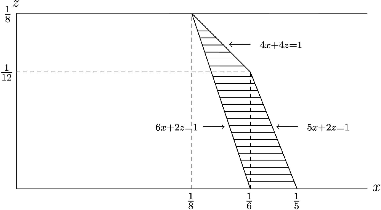
In Figure 1 we show the area in which Mr. Author's proposal would have made sense. The straight diagonal line in Figure 1 gives the lower bound of x for values of z between 0 and  $1/ 8$, while the bent line gives the upper bound for the x-values. For every x and z between these lines, the inequalities (6) are observed. The region in which the Alan Author Effect occurs might perhaps look small, but in fact it is quite large. If
 $z=0$, which corresponds to the strict condition (4), x can be between
 $1/ 6$ and
 $1/ 5$, as can be seen from Figure 1. Since the five triples given in (9) are all equal to one another, their sum can be between
 $5/ 6$ and 1, which is a large part of the whole probability space. True, at the maximum allowed value of
 $z$, namely,
 $1/ 8$, the allowed values for x shrink to the point
 $x=1/ 8$; but at
 $z=1/ 12$, for instance—which corresponds to the kink in the bent line of Figure 1—one finds
 $5/ 36< x< 1/ 6$.
Allowed region of x-z plane for Alan Author Effect.

Appendix A: Proof of Confirmation
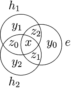
Here is a compact notation for the probabilities of the elementary intersections of the sets  $h_{1},\, h_{2},\, e$, as displayed in Figure 2:


Venn diagram for h 1, h 2, and e.

An important point is that these seven triple probabilities are nonnegative, that is, each one must be positive or zero. Further their sum cannot be larger than unity, for

Under this global condition (10) the seven triple probabilities are independent variables, spanning a hypervolume in seven dimensions.
The purpose of the calculations in this appendix is to show that, under the restrictions  $z_{1}=0=z_{2}$, it is the case that
 $c( h_{1}\wedge h_{2},\, e) \geq c( h_{1},\, e) $ and
 $c( h_{1}\wedge h_{2},\, e) \geq c( h_{2},\, e) $, for all of the nine realizations of the generic measure
 $c$, that is, for
 $C$,
 $D$,
 $S$,
 $Z$,
 $R$,
 $L$,
 $N$,
 $K$,
 $F$. To do this, it will be proved, for each of the measures, that
 $c( h_{1}\wedge h_{2},e) -c( h_{1},e) $ can be reduced to an expression involving the five remaining independent triple probabilities that is manifestly nonnegative. Terms that can be recognized as being nonnegative are of course products of triple probabilities with a plus sign, or terms involving
 $1-\Sigma $, where
 $\Sigma $ is a triple probability or the sum of two or more of them (cf. (10)). Once that has been done, the job is finished, for then
 $c( h_{1}\wedge h_{2},\, e) \geq c( h_{1},\, e) $ has been demonstrated;
 $c( h_{1}\wedge h_{2},\, e) \geq c( h_{2},\, e) $ follows immediately by interchanging the subscripts 1 and 2 throughout the proof.
Let us begin with the Carnap measure  $C$. We read off from the Venn diagram that

Since  $( x+y_{0}) y_{1}$ is manifestly nonnegative, we conclude that
 $C( h_{1}\wedge h_{2},\, e) \geq C( h_{1},\, e) $. This concludes the demonstration for this simple measure.
The Carnap-Eells measure D and Christensen's S are not much harder:

Since  $( x+y_{0}) =P( e) $, given that z 1 = 0 = z 2, and
 $y_{1}=P( h_{1}\wedge \neg h_{2}\wedge $
 $\neg e) $, we have thereby proved inequality (7). Similarly,

For the Z measure of Crupi, Tentori, and Gonzalez, we have to distinguish the cases in which  $P( h_{1}\wedge h_{2}\vert e) $ is larger from those in which it is smaller than
 $P( h_{1}\vert e) $. In the former case,
 $Z( h_{1}\wedge h_{2},\, e) \geq 0$: either
 $Z( h_{1},\, e) < 0$, so
 $Z( h_{1}\wedge h_{2},\, e) > Z( h_{1},\, e) $ trivially, or
 $Z( h_{1},\, e) \geq 0$, and then we find

where  $N_{Z+}$ has the form

which is nonnegative.
The alternative is  $Z( h_{1}\wedge h_{2},\, e) < 0$, and then

so  $Z( h_{1}\wedge h_{2},\, e) < 0$ implies
 $D( h_{1}\wedge h_{2},\, e) < 0$. Since
 $z_{1}=z_{2}=0$, we know that
 $D( h_{1},\, e) \leq D( h_{1}\wedge h_{2},\, e) $, so
 $D( h_{1},\, e) < 0$. Thus
 $Z( h_{1},\, e) < 0$ and we can calculate the difference

where  $N_{Z-}$ is given by

which is also nonnegative. This concludes the proof for the measure  $Z$.
As to the two measures involving logarithms,

 $L$ is a little more complicated, and we find

Nozick's measure yields

where

For the Kemeny-Oppenheim measure,

with the numerator

Similarly, Fitelson's form leads to

where this numerator is

This concludes the proof that (4) is a robust sufficient condition for the validity of (5). However, by scrutinizing the forms that we have obtained for each of the expressions for  $c( h_{1}\wedge h_{2},\, e) -c( h_{1},\, e) $, we observe that, if we add to (4) the requirement that none of the remaining five triple probabilities,
 $x,\, y_{0},\, y_{1},\, y_{2},\, z_{0}$ is zero—which is always a valid option—then the inequalities in (5) can be replaced by strict inequalities, that is,

It is of course interesting that the equality option can be excluded so easily, and moreover robustly, that is, in a manner that works for all the measures considered.
Appendix B: Disconfirmed Hypotheses
In this appendix we will describe sufficient conditions for the validity of the three strict inequalities  $c( h_{1},\, e) < 0$,
 $c( h_{2},\, e) < 0$, and
 $c( h_{1}\wedge h_{2},\, e) > 0$. To do this we will set
 $x=y_{0}=y_{1}=y_{2}=z_{0}$ and
 $z\equiv z_{1}=z_{2}$. Thus five of the marked areas in the Venn diagram are equal to
 $x$, while the remaining two are equal to z. It will be required that x is nonzero, while z may be zero or nonzero, so in this appendix the condition (4) is being relaxed: it will turn out that z should be small, but need not be zero. The reason for reducing the seven-dimensional problem to a two-dimensional one is purely one of convenience. With more trouble, for instance, one could allow
 $z_{1}$ and
 $z_{2}$ to be different. However the purpose here is only to show that the inequalities (6) are possible, not to explore every part of the seven-dimensional hypervolume for which they hold.
Consider first the Carnap confirmation function  $C( h,\, e) $. We read off from the Venn diagram that


If  $1-6x-2z< 0$ and
 $1-4x-4z> 0$, then
 $C( h_{1},\, e) < 0$ and C(h 1∧h 2, e)>0. The first inequality yields
 $6x> 1-2z$, while the second gives
 $4x< 1-4z$, which are consistent with each other if
 $( 1-4z) / 4> ( 1-2z) / 6$, and that is only possible if
 $z< 1/ 8$. When this holds,

In addition, there is the constraint  $x+y_{0}+y_{1}+y_{2}+z_{0}+z_{1}+z_{2}\leq 1$, which means that
 $5x+2z\leq 1$. Note that
 $z=0$ is possible, for then the inequalities simply reduce to
 $1/ 6< x< 1/ 5$. We see that
 $C( h_{1},\, e) < 0$ and
 $C( h_{1}\wedge h_{2},\, e) > 0$ are simultaneously possible, and because of the symmetry between
 $h_{1}$ and
 $h_{2}$, also
 $C( h_{2},\, e) < 0$ (indeed, with the symmetries that we have imposed,
 $C( h_{2},\, e) =C( h_{1},e) $). As we have seen, this can occur under the strict condition (4), but also when this condition is relaxed.
We will now show that these inequalities guarantee  $c( h_{1},\, e) < 0$ and
 $c( h_{1}\wedge h_{2},\, e) > 0$, also when
 $c$ is realized by the other measures of confirmation. This is obvious for
 $D$,
 $S$,
 $N$,
 $K$, and
 $F$ because


Whenever  $C$ is positive (or negative),
 $D,\, S,\, N,\, K$, and
 $F$ are likewise positive (or negative), so the same sufficient conditions are applicable. The same applies to the measure
 $Z$, but we have to distinguish between two cases:

The first form must be used for  $h\equiv h_{1}\wedge h_{2}$, when
 $C$ and
 $Z$ are both positive. The second form is needed for
 $h\equiv h_{1}$, for then
 $C$ and
 $Z$ are negative. We have used the fact that
 $C$,
 $D$,
 $S$,
 $N$, and
 $F$ are all equivalent up to normalization, which indeed inspired Crupi et al. (Reference Crupi, Tentori and Gonzalez2007) to produce their
 $Z$-measure, which has the property that it is equal to 1 if
 $e$ implies
 $h$, and
 $-1$ if e implies
 $\neg h$.
For the logarithmic measures  $R$ and
 $L$ we can write

and

Evidently, when  $C( h,\, e) $ is positive, zero, or negative,
 $R( h,\, e) $ is positive, zero, or negative, respectively, and the same goes for
 $L( h,\, e) $, so our results also extend to these cases. Indeed, the results apply to any (Bayesian) measure of confirmation,
 $c( h,\, e) $, for which

where we understand  $\mathrm{sign}\,[ b] $ to be
 $+1$, 0, or
 $-1$, according to whether
 $b$ is positive, zero, or negative, respectively.
In conclusion, we have proved the following robust result, which we call the Alan Author Theorem: A sufficient condition for  $c( h_{1},\, e) < 0$,
 $c( h_{2},\, e) < 0$ and
 $c( h_{1}\wedge h_{2},\, e) > 0$ is

where  $c$ stands for
 $C,\, D,\, S,\, Z,\, R,\, L,\, N,\, K,\, F$, or any other measure that satisfies (12), and where

The upper bound,  $z\leq 1/ 8$, is in fact already implied by the first part of (13).
Appendix C: Bovens and Hartmann Coherence
In Section 2 it was noted that there is a close conceptual link between confirmation and coherence: measures of confirmation can be put to work as measures of coherence and vice versa. The nine measures of confirmation that we have considered so far were all quantitative, that is, the confirmation that  $e$ gives to
 $h$ is expressed as a number between
 $-1$ and
 $+1$.
Bovens and Hartmann (Reference Bovens and Hartmann2003a, Reference Bovens and Hartmann2003b) have introduced a coherence measure that is comparative rather than quantitative. Given two pairs of propositions, for example  $\{ h,\, e\} $ and
 $\{ h^{\prime },\, e^{\prime }\} $, Bovens and Hartmann describe a condition such that, when it is fulfilled, it tells us which of the two pairs is the more coherent. An ordering of pairs is thus introduced, but it is what Bovens and Hartmann call a quasiordering. For it can happen that the condition is not fulfilled, and then the relative coherence of two different pairs is simply not defined.
In more detail, the quasiordering can be explained as follows. Imagine a witness who reports on a hypothesis and some evidence about which he has heard. Let  $h$ be his report concerning the hypothesis, and
 $e$ be his formulation of the evidence. Define


Consider the function

where x is a number in the interval  $[ 0,\, 1] $ that represents the unreliability of the witness, with 1 corresponding to total unreliability and 0 to total reliability. According to Bovens and Hartmann, the pair
 $\{ h^{\prime },\, e^{\prime }\} $ is not less coherent than the pair
 $\{ h,\, e\} $ if

The salient point is that this inequality must hold for all  $x$, that is, for all possible degrees of unreliability of the witness,
 $x$ being the same for both pairs
 $\{ h^{\prime },\, e^{\prime }\} $ and
 $\{ h,\, e\} $. If (15) holds with
 $\geq $ replaced by
 $\leq $, then
 $\{ h^{\prime },\, e^{\prime }\} $ is said to be not more coherent than the pair
 $\{ h,\, e\} $. However, it can happen that (15) holds neither with ≥ nor with ≤, and then the relative coherence of the two pairs is undefined: they are not ordered in respect of their Bovens-Hartmann coherence.
Bovens and Hartmann illustrate cases in which the inequality (15) holds by means of a graph that shows the left- and the right-hand sides as curves that do not intersect one another. Here we introduce, however, a simple algebraic alternative. Since  $a_{2}=1-a_{0}-a_{1}$, it follows from (14) that

Further, since the left-hand side of this equation is a monotonic increasing function of  $B( h,\, e\mathrm{;}\,x) \in [ 0,\, 1] $, for fixed
 $x$, it follows that (15) is equivalent to

With the notation  $X=x^{2}$, this can be rewritten

The above inequality holds at  $X=0$ if
 $a^{\prime }_{0}/ a^{\prime }_{1}\geq a_{0}/ a_{1}$, and it holds at
 $X=1$ if
 $1/ a^{\prime }_{1}\geq 1/ a_{1}$. This is a necessary and sufficient condition such that the two straight lines in (17), to the left and right of
 $\geq $, do not cross, and therefore that (16) is true. These requirements are equivalent to

We now set  $h=h_{1}$,
 $h^{\prime }=h_{1}\wedge h_{2}$,
 $e^{\prime }=e$; and we use Bovens-Hartmann coherence as a (relative) measure of confirmation. Conditions (18) read

On referring to the Venn diagram of Appendix A, we transcribe these conditions as follows:

which reduce respectively to

Evidently both of these equalities are satisfied automatically if  $z_{2}=0$. Under this condition we conclude that
 $h_{1}\wedge h_{2}$ is not less highly Bovens-Hartmann confirmed by
 $e$ than is
 $h_{1}$ alone. A similar argument—with
 $h_{1}$ and
 $h_{2}$ interchanged—shows that if
 $z_{1}=0$,
 $h_{1}\wedge h_{2}$ is not less highly confirmed by
 $e$ than is
 $h_{2}$ alone.
Since  $z_{1}=0=z_{2}$ is equivalent to the conditions (4) of Section 2, we have shown thereby that the robustness of these conditions extends also to the measure of Bovens and Hartmann. Moreover, if neither
 $x$ nor
 $y_{1}$ nor
 $y_{2}$ is zero, ≤ may be replaced by < , and under these conditions
 $h_{1}\wedge h_{2}$ is strictly more confirmed by
 $e$ than are
 $h_{1}$ or
 $h_{2}$.
The work of this appendix may be seen as an extension of Appendix A to Bovens-Hartmann confirmation. No analogous extension in the spirit of Appendix B is possible, for it does not make sense to say that  $h_{1}\wedge h_{2}$ is confirmed, nor that
 $h_{1}$ or
 $h_{2}$ are disconfirmed in the sense of Bovens and Hartmann.