Introduction
To anticipate and mitigate the impacts of anthropogenic greenhouse warming over the next few centuries, we need to understand how climate change may impact the biogeographic ranges, speciation potential, and extinction risk of organisms. In addition to increasing temperatures, a warming ocean will experience changes in oxygenation level, acidification, carbon cycling, ocean circulation patterns, sea level, and habitat distributions, among other parameters. Some of these effects will be global in their impact whereas others will vary from region to region (Intergovernmental Panel on Climate Change [IPCC] 2013). These changes have the potential to alter the geographic distributions of marine organisms and influence their processes of origination and extinction.
The relationships among global warming, sea-level rise, geographic distributions, and biodiversity of mobile marine animals are not well understood. Two end-member models of these relationships are proposed here. On one hand, increasing sea level and a reduced latitudinal temperature gradient might promote dispersal of marine species through newly opened marine corridors and to higher latitudes, leading to larger geographic ranges, poleward latitudinal shifts, decreased speciation, and a drop in biodiversity (as argued, for instance, by Monnet et al. Reference Monnet, Bucher, Escarguel and Guex2003). On the other hand, increasing sea level may form new, isolated epicontinental basins, resulting in faunal endemism, smaller geographic ranges, increased speciation, and an increase in biodiversity (Yacobucci Reference Yacobucci1999; Courville Reference Courville2007). Several observations further complicate these two end-member models. Wider geographic ranges are often associated with reduced extinction probabilities (Payne and Finnegan Reference Payne and Finnegan2007; Landman et al. Reference Landman, Goolaerts, Jagt, Jagt-Yazykova, Machalski and Yacobucci2014; Foote et al. Reference Foote, Ritterbush and Miller2016), though Myers et al. (Reference Myers, MacKenzie and Lieberman2013) found no relationship between range size and extinction probability for Late Cretaceous mollusks from the Western Interior Seaway (WIS). Lagomarcino and Miller (Reference Lagomarcino and Miller2012) found a correlation between generic diversity and increasing area of epicontinental seas in Late Cretaceous marine invertebrates, and Foote (Reference Foote2014) found marine animal genera generally increased their geographic ranges in concert with increases in the area of their preferred habitat. However, increasing sea level need not always result in increased shelf area (Holland Reference Holland2012; Holland and Christie Reference Holland and Christie2013). Furthermore, investigation of oxygen demands of modern marine ectotherms suggests that the anoxia associated with warmer ocean temperatures may cause the geographic ranges of taxa to constrict in order to maintain a suitable balance of oxygen supply versus resting metabolic oxygen demand (Deutsch et al. Reference Deutsch, Ferrell, Seibel, Pörtner and Huey2015). The complexity and interconnectedness of these causal processes make it difficult to predict how greenhouse warming has and will affect marine habitats and the distribution and diversity of marine life. It is therefore essential to explore and test these models with rich empirical data for marine animals from ancient greenhouse episodes to determine which processes and which relationships actually controlled biodiversity.
The Cenomanian and Turonian (C–T; 100.5–89.8 Ma) stages of the Late Cretaceous represent just such a critical interval in Earth history. Global sea level increased during the Cenomanian to reach a Phanerozoic peak near the C/T boundary (93.9 Ma) before decreasing in the middle and late Turonian (Hancock and Kauffman Reference Hancock and Kauffman1979; Haq et al. Reference Haq, Hardenbol and Vail1987; Hay Reference Hay1995). This sea-level rise flooded large areas of the continents to produce extensive epicontinental seas (Hancock and Kauffman Reference Hancock and Kauffman1979; Hay Reference Hay1995, Reference Hay2008). Carbon dioxide levels in the atmosphere were elevated (Arthur et al. Reference Arthur, Dean and Schlanger1985; Berner Reference Berner1994; Berner and Kothavala Reference Berner and Kothavala2001; Bice and Norris Reference Bice and Norris2002; Bice et al. Reference Bice, Birgel, Meyers, Dahl, Hinrichs and Norris2006; Poulsen et al. Reference Poulsen, Tabor and White2015), producing significant global greenhouse warming (Huber et al. Reference Huber, Hodell and Hamilton1995, Reference Huber, Norris and MacLeod2002; Herman and Spicer Reference Herman and Spicer1996; Clarke and Jenkyns Reference Clarke and Jenkyns1999; Wilson and Norris Reference Wilson and Norris2001; Norris et al. Reference Norris, Bice, Magno and Wilson2002; Jenkyns Reference Jenkyns2003; Eleson and Bralower Reference Eleson and Bralower2005; Forster et al. Reference Forster, Schouten, Baas and Sinninghe Damsté2007a,Reference Forster, Schouten, Moriya, Wilson and Sinninghe Damstéb; Moriya et al. Reference Moriya, Wilson, Friedrich, Erbacher and Kawahata2007; Friedrich et al. Reference Friedrich, Norris and Erbacher2012). Poulsen et al. (Reference Poulsen, Tabor and White2015) modeled Cenomanian climate, citing likely values of high (1120 ppmv) atmospheric CO2, low (10%) atmospheric O2, and a high (21.5°C) global average surface temperature. Temperatures peaked during the Turonian, with tropical sea surface temperatures as high as 33–36°C (Clarke and Jenkyns Reference Clarke and Jenkyns1999; Norris et al. Reference Norris, Bice, Magno and Wilson2002; Forster et al. Reference Forster, Schouten, Moriya, Wilson and Sinninghe Damsté2007b). This interval of high sea levels and greenhouse warming was briefly interrupted in the middle Cenomanian substage and again in the middle Turonian substage, when global sea level fell (~25–45 m; Miller et al. Reference Miller, Wright and Browning2005) and temperatures cooled (~3°C; Miller et al. Reference Miller, Wright and Browning2005), likely within less than 400,000 years (Paul et al. Reference Paul, Mitchell, Marshall, Leary, Gale, Duane and Ditchfield1994; Hancock Reference Hancock2003; Miller et al. Reference Miller, Wright and Browning2005; Bice et al. Reference Bice, Birgel, Meyers, Dahl, Hinrichs and Norris2006; Forster et al. Reference Forster, Schouten, Baas and Sinninghe Damsté2007a; Giraud et al. Reference Giraud, Reboulet, Deconinck, Martinez, Carpentier and Bréziat2013).
In concert with sea-level rise and greenhouse warming, an oceanic anoxic event (OAE2) occurred near the C/T boundary, reflecting one of the largest carbon-cycle perturbations of the Mesozoic (Schlanger and Jenkyns Reference Schlanger and Jenkyns1976; Arthur and Schlanger Reference Arthur and Schlanger1979; Jenkyns Reference Jenkyns1980, Reference Jenkyns2010; Pratt Reference Pratt1984, Reference Pratt1985; Arthur et al. Reference Arthur, Schlanger and Jenkyns1987, Reference Arthur, Dean and Pratt1988; Schlanger et al. Reference Schlanger, Arthur, Jenkyns and Scholle1987; Bralower Reference Bralower1988; Jarvis et al. Reference Jarvis, Carson, Cooper, Hart, Leary, Tocher, Horne and Rosenfeld1988, Reference Jarvis, Gale, Jenkyns and Pearce2006, Reference Jarvis, Lignum, Gröcke, Jenkyns and Pearce2011; Gale et al. Reference Gale, Jenkyns, Kennedy and Corfield1993; Kaiho and Hasegawa Reference Kaiho and Hasegawa1994; Hasegawa Reference Hasegawa1997; Uličny et al. Reference Uličny, Hladikova, Attrep, Čech, Hradecká and Svobodová1997; Leckie et al. Reference Leckie, Bralower and Cashman2002; Bowman and Bralower Reference Bowman and Bralower2005; Sageman et al. Reference Sageman, Meyers and Arthur2006; Turgeon and Creaser Reference Turgeon and Creaser2008; Monteiro et al. Reference Monteiro, Pancost, Ridgwell and Donnadieu2012; Elderbak et al. Reference Elderbak, Leckie and Tibert2014; van Helmond et al. Reference Van Helmond, Sluijs, Sinninghe Damsté, Reichart, Voigt, Erbacher, Pross and Brinkhuis2015; Elderbak and Leckie Reference Elderbak and Leckie2016; Zheng et al. Reference Zheng, Jenkyns, Gale, Ward and Henderson2016; Jenkyns et al. Reference Jenkyns, Dickson, Ruhl and Van Den Boorn2017). During this interval, oxygen-deficient bottom waters spread widely, and burial rates of organic carbon were increased, resulting in the extensive deposition of organic-rich black shales. Carbon isotopic records in many regions of the world show a strong positive excursion in δ13C values in the latest Cenomanian, reflecting increased burial of organic carbon (Pratt Reference Pratt1985; Schlanger et al. Reference Schlanger, Arthur, Jenkyns and Scholle1987; Gale et al. Reference Gale, Jenkyns, Kennedy and Corfield1993; Huber et al. Reference Huber, Hodell and Hamilton1995; Hasegawa Reference Hasegawa1997; Uličny et al. Reference Uličny, Hladikova, Attrep, Čech, Hradecká and Svobodová1997; Bowman and Bralower Reference Bowman and Bralower2005; Jarvis et al. Reference Jarvis, Gale, Jenkyns and Pearce2006, Reference Jarvis, Lignum, Gröcke, Jenkyns and Pearce2011; Sageman et al. Reference Sageman, Meyers and Arthur2006; Forster et al. Reference Forster, Schouten, Baas and Sinninghe Damsté2007a,Reference Forster, Schouten, Moriya, Wilson and Sinninghe Damstéb). The causal mechanism for OAE2 has been debated for decades and would certainly have entailed a complex set of Earth-system processes. The most often-cited explanation involves increased volcanism (in particular more extensive and faster-spreading midocean ridges plus emplacement of large igneous provinces) injecting CO2 into the atmosphere. The resulting greenhouse warming led to higher sea levels, which increased areas of upwelling. The resulting increased marine primary productivity expanded the oxygen minimum zone (Arthur et al. Reference Arthur, Schlanger and Jenkyns1987; Premoli Silva et al. Reference Premoli Silva, Erba, Salvini, Locatelli and Verga1999; Wilson and Norris Reference Wilson and Norris2001; Leckie et al. Reference Leckie, Bralower and Cashman2002; Martin et al. Reference Martin, MacLeod, Jiménez Berrocoso and Bourbon2012; Monteiro et al. Reference Monteiro, Pancost, Ridgwell and Donnadieu2012). Others have suggested that increased midocean ridge volcanism would also result in more hydrothermal activity, supplying micronutrients that helped fuel increased productivity (Leckie et al. Reference Leckie, Bralower and Cashman2002), and that the key driver was not absolute sea-level height but the area of newly flooded shallow shelf (Uličny et al. Reference Uličny, Hladikova, Attrep, Čech, Hradecká and Svobodová1997). Alternatively, others have argued for low productivity in oligotrophic surface waters, driven by increased water-column stratification and lower dissolved oxygen in a warming ocean (Bowman and Bralower Reference Bowman and Bralower2005; Eleson and Bralower Reference Eleson and Bralower2005). It has also been suggested that different ocean basins may have experienced different conditions leading up to and during OAE2, even though the anoxic event appears to be global in nature (Thomas and Tilghman Reference Thomas and Tilghman2014). Evidence exists for a brief (<60-Kyr) cooling episode, the Plenus cold event, early in OAE2 (during the M. geslinianum ammonite zone of the late Cenomanian) tied to the drawdown of atmospheric CO2 as carbon burial increased (Jenkyns Reference Jenkyns2003; Forster et al. Reference Forster, Schouten, Moriya, Wilson and Sinninghe Damsté2007b; Jarvis et al. Reference Jarvis, Lignum, Gröcke, Jenkyns and Pearce2011; van Helmond et al. Reference Van Helmond, Sluijs, Reichart, Sinninghe Damsté, Slomp and Brinkhuis2014; Jenkyns et al. Reference Jenkyns, Dickson, Ruhl and Van Den Boorn2017). This cool episode was short-lived, however, as continuing volcanism quickly caught back up and greenhouse warming resumed (Forster et al. Reference Forster, Schouten, Moriya, Wilson and Sinninghe Damsté2007b; Jarvis et al. Reference Jarvis, Lignum, Gröcke, Jenkyns and Pearce2011).
Associated with OAE2 is the C/T extinction event. Raup and Sepkoski (Reference Raup and Sepkoski1986) identified this interval as one of the 10 largest extinctions of the Phanerozoic, affecting a range of marine organisms, including planktic and benthic microorganisms (calcareous nannoplankton, radiolarians, benthic and planktic foraminifera; Kaiho and Hasegawa Reference Kaiho and Hasegawa1994; Premoli Silva et al. Reference Premoli Silva, Erba, Salvini, Locatelli and Verga1999; Leckie et al. Reference Leckie, Bralower and Cashman2002; Elderbak et al. Reference Elderbak, Leckie and Tibert2014; Kaiho et al. Reference Kaiho, Katabuchi, Oba and Lamolda2014) and metazoans (Elder Reference Elder1989; Harries Reference Harries1993; Harries and Little Reference Harries and Little1999; Hirano et al. Reference Hirano, Toshimitsu, Matsumoto and Takahashi2000; Monnet et al. Reference Monnet, Bucher, Escarguel and Guex2003; Monnet and Bucher Reference Monnet and Bucher2007b; Monnet Reference Monnet2009; Jagt-Yazykova Reference Jagt-Yazykova2011, Reference Jagt-Yazykova2012; Kurihara et al. Reference Kurihara, Toshimitsu and Hirano2012; Brom et al. Reference Brom, Salamon, Ferré, Brachaniec and Szopa2015). Interestingly, some groups show elevated rates of both extinction and origination during the anoxic event (Leckie et al. Reference Leckie, Bralower and Cashman2002). Although generally considered to be a significant turnover event in marine ecosystems, some have suggested that the apparent extinction at the C/T boundary is a preservational artifact. Gale et al. (Reference Gale, Smith, Monks, Young, Howard, Wray and Huggett2000) and Smith et al. (Reference Smith, Gale and Monks2001) argued that the rapid sea-level rise in the late Cenomanian resulted in the spread of more oligotrophic waters onto the northwestern European shelf, causing a shift in both lithology and faunal composition. Shallow-water communities, they argue, were displaced inland; when sea level fell again, these deposits were exposed to erosion, leaving a gap in the rock and fossil records. Although this bias may be significant regionally in the Anglo-Paris Basin, it does not appear to apply in other regions, where the progressive spread of stressed conditions and associated extinctions from offshore to onshore environments are well documented (e.g., Elder Reference Elder1989; Kaiho and Hasegawa Reference Kaiho and Hasegawa1994; Elderbak et al. Reference Elderbak, Leckie and Tibert2014; Kaiho et al. Reference Kaiho, Katabuchi, Oba and Lamolda2014).
It has been suggested that cephalopod mollusks may show particularly rapid changes in abundance and diversity due to global warming and associated changes in marine conditions, in part because of the accelerated life histories that many modern cephalopod species show (Doubleday et al. Reference Doubleday, Prowse, Arkhipkin, Pierce, Semmens, Steer, Leporati, Lourenço, Quetglas, Sauer and Gillanders2016). Cephalopods, especially ammonoids, were globally widespread and very diverse during the C–T interval. Their response to OAE2 and the C/T extinction event, however, has not been clear. Ammonoids in general show very rapid rates of origination and extinction (Yacobucci Reference Yacobucci2005, Reference Yacobucci2015), and it can be difficult to separate background turnover from more pronounced extinction events. Elder (Reference Elder1989), Harries (Reference Harries1993), and Harries and Little (Reference Harries and Little1999) reported levels of ammonoid extinction in the WIS of North America across the C/T as high as 74–95% of species eliminated but with a rapid recovery in the early Turonian. Nektobenthic ammonoids were harder hit than pelagic groups (Elder Reference Elder1989; Harries and Little Reference Harries and Little1999). Other workers have reported high levels of ammonoid extinction across the C/T in Japan (Hirano et al. Reference Hirano, Toshimitsu, Matsumoto and Takahashi2000) and Pacific Russia (Jagt-Yazykova Reference Jagt-Yazykova2011, Reference Jagt-Yazykova2012). On the other hand, recent work has suggested that ammonoid turnover may not be so pronounced during the late Cenomanian and early Turonian. Monnet and colleagues have documented ammonoid diversity through the C–T interval in northwest Europe, Tunisia, and the WIS (Monnet and Bucher Reference Monnet and Bucher2002, Reference Monnet and Bucher2007a,Reference Monnet and Bucherb; Monnet et al. Reference Monnet, Bucher, Escarguel and Guex2003; Monnet Reference Monnet2009). They found that, in Europe, ammonoid species richness actually declined between the middle and late Cenomanian substages, before peak sea level and OAE2, with pelagic heteromorphs becoming extinct before nektobenthic acanthoceratid ammonoids (Monnet et al. Reference Monnet, Bucher, Escarguel and Guex2003; Monnet and Bucher Reference Monnet and Bucher2007b). This crisis near the middle–late Cenomanian boundary is supported by Giraud et al. (Reference Giraud, Reboulet, Deconinck, Martinez, Carpentier and Bréziat2013), who found turnover of ammonoids in France in association with middle Cenomanian cooling and rapid sea-level changes, and Kurihara et al. (Reference Kurihara, Toshimitsu and Hirano2012), who found ammonoid diversity dropped near the middle–late Cenomanian boundary in Japan. At the C/T boundary, diversity dropped only modestly (and less than it did across the middle–late Cenomanian boundary) in Europe, whereas diversity stayed high in the WIS and actually peaked in the early Turonian in Tunisia (Monnet Reference Monnet2009). Hence, Monnet and colleagues argued that the C/T turnover event was not global and that widespread anoxia was not sufficient to decrease ammonoid diversity. Instead, Monnet et al. (Reference Monnet, Bucher, Escarguel and Guex2003) argued that rising sea levels in the middle Cenomanian led to decreased geographic isolation and therefore reduced rates of speciation, resulting in the net drop in ammonoid diversity. Whether this pattern is specific to Europe or reflects diversity dynamics globally is an open question.
Here I evaluate the two models for biodiversity change in a greenhouse interval by investigating cephalopod diversity changes through the C–T interval using a larger, longer, and more global database than previous workers. Did greenhouse warming and sea-level rise promote dispersal, increase geographic ranges, and decrease speciation in C–T cephalopods? Or did these changes result in increased endemism and evolutionary radiation within newly formed epicontinental seaways? To address these questions requires documenting and assessing changes in diversity, latitudinal distributions, geographic range sizes, and provincialism versus cosmopolitanism throughout the C–T interval, both globally and comparatively among different regions and different cephalopod clades.
Materials and Methods
Fossil Occurrence Data
Fossil occurrences of cephalopods from the Cenomanian and Turonian stages of the Late Cretaceous were extracted from two data sets, the Paleobiology Database (PBDB) and a data set for Late Cretaceous cephalopods originally compiled from the literature and U.S. Geological Survey (USGS) records by Richard MacKenzie (MKDB) as the basis for his M.S. thesis (MacKenzie Reference MacKenzie2007). The records of fossil occurrences within the MKDB were derived primarily from the literature, including USGS publications, journal articles, monographs, and field guides; a small proportion of the occurrences involve specimens located in museum collections that were not otherwise published. Original data sources for the MKDB are listed in the Supplementary Appendix. Data from the PBDB were downloaded on 2 June 2014, using the search terms “Cenomanian–Turonian” and “Cephalopoda.” The two data sets were then combined. If a fossil occurrence was recorded in both data sets, the MKDB entry was retained, as the MKDB included additional data fields not present in the PBDB data. The data were screened for typographical errors, spelling variations (e.g., T. glabrum vs. T. glabrus), and taxonomic consistency. Where entries had similar genus or species names, the primary systematic literature was used to confirm their distinction or update records to the genus or species name in current use. Occurrences with ambiguous genus and species identifications (e.g., taxa with aff., cf., ex gr., sp., spp., or ? modifiers) were removed from the data set. Occurrences without stratigraphic resolution to the substage level (e.g., early vs. middle vs. late Cenomanian) or sufficient locality information to determine modern latitude and longitude were also excluded.
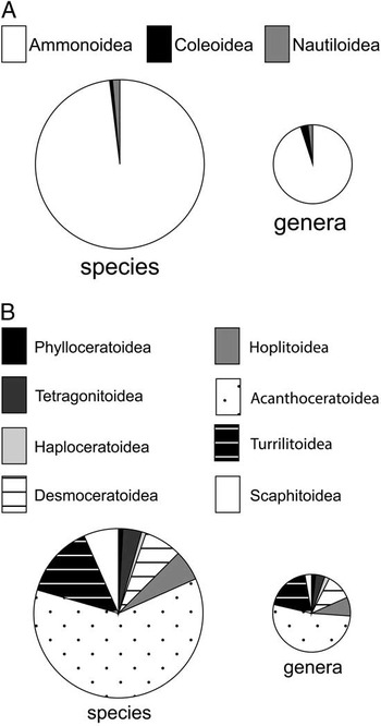
After screening and revisions, a total of 7262 occurrences for 164 genera and 754 species were included in the final data set (77% from the MKDB and 23% from the PBDB), which is available as Supplementary Table 1. The majority of the database is composed of ammonoids (99.4% of occurrences, 98.1% of species, 95.1% of genera), with far fewer nautiloids (0.4% of occurrences, 1.2% of species, 1.8% of genera) or coleoids (0.2% of occurrences, 0.7% of species, 3.0% of genera) (Fig. 1A). Within Ammonoidea, the superfamilies Acanthoceratoidea (60.1% of occurrences and species, 50.0% of genera) and Turrilitoidea (11.0% of occurrences, 13.5% of species, 17.7% of genera) predominate (Fig. 1B).
Taxonomic composition of the data set. A, Cephalopod taxa by subclass. B, Ammonoid taxa by superfamily.

The data were divided into six time intervals, corresponding to stratigraphic substages (i.e., early, middle, and late Cenomanian and early, middle, and late Turonian). Some previous work on the C–T interval has used finer temporal scales, such as ammonoid biozones or subzones (Monnet and Bucher Reference Monnet and Bucher2007b; Monnet Reference Monnet2009). These previous studies, however, focused on just one or a few well-studied regions that have clearly defined biostratigraphic schemes. As the present study uses a globally derived database that includes many more fossil cephalopod occurrences than previous studies, including occurrences from poorly documented regions and/or that cannot be assigned reliably to an ammonoid biozone, the substage was chosen as the finest practicable temporal unit. Durations for each substage were calculated via interpolation from radiometric dates from Cobban et al. (Reference Cobban, Walaszczyk, Obradovich and McKinney2006) and Cohen et al. (Reference Cohen, Finney, Gibbard and Fan2013) (Table 1). Durations for each substage are similar, ranging from 0.9 to 1.8 Myr, with the exception of the early Cenomanian, which is considerably longer (4.4 Myr). If the younger Albian/Cenomanian boundary age (97.2 Ma vs. 100.5 Ma) reported by Scott et al. (Reference Scott, Oboh-Ikuenobe, Benson and Holbrook2009) is used, however, the duration of the early Cenomanian becomes 1.1 Myr, closer to that of the other substages. Sampling from each time slice was relatively consistent, with 1144 to 1698 occurrences per substage, except for the late Turonian, which had significantly fewer occurrences (602) than the other time intervals (Table 1). This reduced number of occurrences for the late Turonian may partly be explained by a sea-level fall that happened through the late Turonian, reducing the size of the WIS (Nielsen et al. Reference Nielsen, Schröder-Adams, Leckie, Haggart and Elderbak2008) and thereby decreasing the extent of shallow-marine rocks from which most cephalopod fossils are recovered. Results for the late Turonian should therefore be interpreted with caution. The number of genera included per substage ranged from 41 to 78 (median=57) and the number of species ranged from 99 to 224 (median=152) (Table 1). As expected given their high evolutionary volatility, the majority of cephalopod species (80.6%) occur in a single substage; 55.5% of genera, on the other hand, occur in more than one substage.
Durations and numbers of cephalopod genera, species, and occurrences in the database for each of six time intervals. Substage durations are derived by interpolation from radiometric dates reported in Cobban et al. (Reference Cobban, Walaszczyk, Obradovich and McKinney2006) and Cohen et al. (Reference Cohen, Finney, Gibbard and Fan2013). Note the long duration of the early Cenomanian; if the younger Albian/Cenomanian boundary date (97.2 Ma vs. 100.5 Ma) of Scott et al. (Reference Scott, Oboh-Ikuenobe, Benson and Holbrook2009) is used, the duration becomes 1.1 Myr, closer to that of the other substages. Rows do not sum to the total for species and genera because 19.4% of species and 55.5% of genera occur in more than one time interval. Cen, Cenomanian; Tur, Turonian.

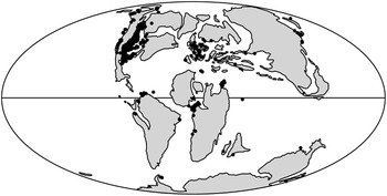
Geographic localities were georeferenced using Google Earth to determine modern latitude and longitude in decimal degrees for each occurrence, typically to within the nearest tenth of 1° or better. These coordinates were entered into the software program PointTracker, Version 4c (Scotese Reference Scotese2001) and rotated to their corresponding paleolatitude and paleolongitude using the 90 Ma plate reconstruction. Accuracy of paleocoordinates was confirmed by plotting the occurrences on a 90 Ma global paleogeographic reconstruction in ArcGIS (Blakey Reference Blakey2011; Environmental Systems Research Institute [ESRI] 2011; Fig. 2). Paleocoordinates were first projected onto a global Mollweide equal-area coordinate system in ArcGIS. The 90 Ma paleogeographic reconstruction was then georeferenced to the modern Mollweide projection using nine linking points. Total root-mean-square error for the georeferenced points was ~52 km, which was deemed satisfactory given the global span of the map and the pixel size of the base-map raster (30 km). The majority of occurrences (79.5%) are from North America, which is the focus of the MKDB, although there is significant coverage of other important C–T regions (e.g., Europe: 9.0%; Africa: 4.7%; South America: 3.3%; Asia: 3.1%), largely derived from the PBDB. Whereas the percentage of occurrences is much greater for North America, the number of occurrences in other regions is still quite high, given the large size of the data set, such that there are sufficient data points to make meaningful interpretations of global patterns.
Paleogeographic map of Cenomanian–Turonian cephalopod occurrences. Base map in equal-area Mollweide projection for 90 Ma (Late Cretaceous) from Blakey (Reference Blakey2011).

To evaluate regional differences in the response of C–T cephalopods to global environmental changes, fossil occurrences were divided into six regions: (1) European Platform, including western and central Europe; (2) Pacific, including the western coast of North America, Peru, Pacific Russia, and Japan; (3) South Atlantic, including the Caribbean, northern and eastern South America, and West Africa; (4) Southern Ocean, including Madagascar, India, Australia, New Zealand, and Antarctica; (5) Tethys, including North Africa, the Middle East, southeastern Europe, and central Asia; (6) WIS, including north-central Mexico and the central United States and central Canada east of 85°W paleolongitude. Definitions of these regions are based on literature documenting biogeographic provinces in the early Late Cretaceous (for review, see Yacobucci Reference Yacobucci2015). The number of cephalopod occurrences in each region varies, from a low of only 33 occurrences in the Southern Ocean to a high of 5786 occurrences in the WIS (Table 2). The European Platform is well represented for the Cenomanian, but the number of occurrences drops off in the Turonian. By contrast, the Pacific, South Atlantic, and Tethys are best sampled in the early Turonian. Numbers of genera (Table 3) and species (Table 4) sampled from each region generally reflect the same trends. Overall, sample sizes from most regions are sufficient to produce robust quantitative comparisons. Tethys and the Southern Ocean have smaller samples, suggesting that more caution in interpreting results from these regions is warranted.
Number of cephalopod fossil occurrences in each of six regions and six time intervals. Cen, Cenomanian; Tur, Turonian.

Number of cephalopod genera occurring in each of six regions and six time intervals. Note that total number of unique genera found in a region is not the sum across the six time intervals, as the same genus may occur in more than one time interval. Cen, Cenomanian; Tur, Turonian.

Number of cephalopod species occurring in each of six regions and six substages. Note that total number of unique species found in a region is not the sum across the six time intervals, as the same species may occur in more than one time interval. Cen, Cenomanian; Tur, Turonian.

Quantifying Diversity and Biogeography
Global diversity was quantified using raw species and genus richness for each of the six time intervals as well as richness values derived from rarefaction analysis in PAST, Version 3.11 (Hammer et al. Reference Hammer, Harper and Ryan2001), treating each substage as a sample and standardizing to the late Turonian (i.e., the substage with the fewest fossil occurrences). To assess regional diversity trends, taxon counts and rarefaction analyses were repeated for each region separately; in these cases, standardization was to whichever time interval had the fewest occurrences. Standard errors for species and genus counts were calculated as the square root of the raw value (appropriate when counts are assumed to be drawn from a Poisson distribution).
Latitudinal distributions for each genus in each time interval were characterized by minimum, median, and maximum paleolatitude coordinates and by the latitudinal range (maximum − minimum paleolatitude). The median values of each of these four metrics were then computed separately for each ammonoid superfamily in each time interval. Computations were repeated for each of the six geographic regions separately to assess differences in regional response. Latitudinal distributions were also calculated separately for the most diverse ammonoid superfamily, Acanthoceratoidea, in each region and each time interval.
The geographic range of each genus in each time interval was estimated as the area (in square kilometers) of a convex-hull bounding point occurrences. Fossil occurrence data were imported into ArcMap, Version 10.1 (ESRI 2011) and projected with the equal-area Mollweide projection. Layers were constructed for each of the six time intervals, with fossil occurrences represented as points. For each time interval, the “minimum bounding geometry” data-management tool in ArcMap was used to extract the area of the convex hull on the projection for each genus’s occurrences. The areas were then log10 transformed to reduce the large range of area values and to compare areas in terms of order of magnitude. For taxa with only a single occurrence, the area was set conservatively to 10 km2, such that the log10 area was 1. For taxa with two occurrences, the area was set to two times the distance between points, then log10 transformed; this approach ensured that taxa with two occurrences were almost always assigned a larger area than taxa with a single occurrence.
Latitudinal distributions and geographic area measures were nonnormally distributed, so differences were evaluated using nonparametric pairwise Mann-Whitney U-tests. Two correction methods for multiple comparisons were used, the more conservative post hoc sequential Bonferroni correction in PAST, Version 3.11 (Hammer et al. Reference Hammer, Harper and Ryan2001) and the less conservative false discovery rate (Benjamini and Hochberg Reference Benjamini and Hochberg1995) using the Excel calculator developed by Weinkauf (Reference Weinkauf2012). In most cases, the two methods produced the same results; where they differ, this is noted in the text. Details of the results of U-tests showing significant differences are given in the text. Details of those comparisons with no significant differences are omitted here, but full results of all tests are provided in Supplementary Table 2.
Finally, to capture changes in the degree of restricted (i.e., provincial) versus cosmopolitan biogeographic distributions through time and among regions, each genus in each time interval and each region was assigned to one of three categories: (1) all occurrences restricted to a single region, (2) occurrences in two regions, or (3) occurrences in three or more regions. These assignments were then used to determine whether the percentage of restricted versus cosmopolitan genera changed over time and whether certain regions showed a higher percentage of provincialism or cosmopolitanism than others.
Results
Diversity
Global patterns of diversity change through the C–T interval are presented first, followed by assessment of diversity changes within each of the six defined regions.
Global Diversity
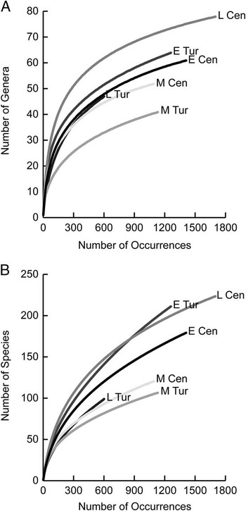
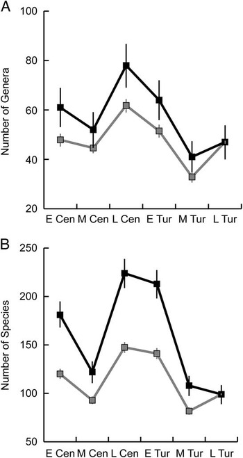
The shapes of the rarefaction curves suggest adequate sampling for both species and genera for most time intervals (Fig. 3). Possible exceptions are species sampling in the early and late Turonian intervals (Fig. 3B), where the rarefaction curves are somewhat less convex, which may suggest that sampling has not arrived at saturation. Whether considering raw or rarified global cephalopod taxon counts, both species- and genus-level diversity were relatively low in the middle Cenomanian, then peaked in the late Cenomanian before declining through the early and middle Turonian (Fig. 4). The diversity drop across the C/T boundary was slight, with the early Turonian maintaining relatively high diversity overall. It is not until the middle Turonian that diversity became notably low.
Global rarefaction curves for cephalopod species and genera in six substages of the Cenomanian–Turonian interval. A, Generic richness. B, Species richness. E Cen, early Cenomanian; M Cen, middle Cenomanian; L Cen, late Cenomanian; E Tur, early Turonian; M Tur, middle Turonian; L Tur, late Turonian.

Raw (black) and rarified (gray) global taxon counts for cephalopod species and genera through the Cenomanian–Turonian interval. A, Generic richness. B, Species richness. Error bars reflect standard error estimated as the square root of the raw values (raw) or the square root of resampling variances (rarified). Substage abbreviations as in Fig. 3.

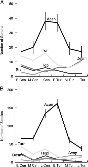
Different cephalopod groups show different diversity patterns through the C–T interval (Fig. 5). Acanthoceratoidea was by far the most diverse superfamily at the species and genus level and shows considerably more changes in diversity through time than other cephalopod groups. Diversity was relatively low in the early and middle Cenomanian before climbing sharply in the late Cenomanian. Whereas acanthoceratoid generic richness dropped slightly across the C/T boundary (from 38 to 37 genera), species richness actually increased (from 134 to 162) before declining dramatically (to 60) in the middle Turonian. Scaphitoidea shows a similar pattern, with no change in generic richness and a modest increase (from 10 to 12) in species across the C/T boundary. Desmoceratoidea, on the other hand, shows a modest increase in genera (from 3 to 6) and decrease in species (from 10 to 8) across the C/T boundary, with a jump up in generic richness through the Turonian. Other cephalopod groups show a decline in both generic and species richness from the late Cenomanian to early Turonian substages (Turrilitoidea, Hoplitoidea, Tetragonitoidea) or very little change through time (Haploceratoidea, Phylloceratoidea, Nautiloidea, Coleoidea).
Raw global taxon counts for the five most abundant cephalopod superfamilies through the Cenomanian–Turonian interval. A, Generic richness. B, Species richness. Error bars (calculated as in Fig. 4) are provided for Acanthoceratoidea but omitted for other superfamilies for clarity. Acan, Acanthoceratoidea; Turr, Turrilitoidea; Desm, Desmoceratoidea; Hopl, Hoplitoidea; Scap, Scaphitoidea. Substage abbreviations as in Fig. 3.

Regional Diversity
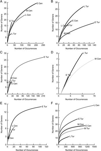
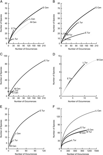
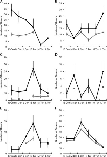
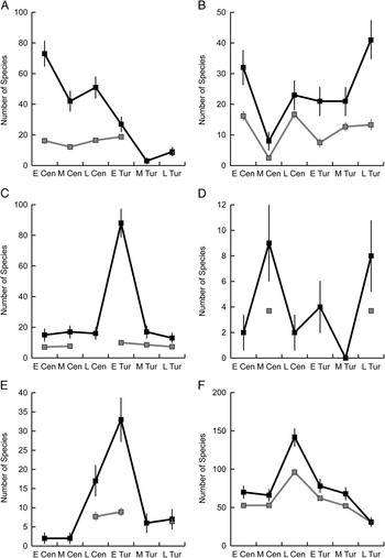
Rarefaction curves for genera (Fig. 6) and species (Fig. 7) indicate adequate sampling for some but not all regions at different times. The Southern Ocean (Figs. 6D, 7D) is particularly poorly sampled, as are the South Atlantic and Tethys, except during the early Turonian (Figs. 6C,E, 7C,E). The European Platform (Figs. 6A, 7A), Pacific (Figs. 6B, 7B), and especially the WIS (Figs. 6F, 7F) show more even sampling through time. Patterns of genus (Fig. 8) and species (Fig. 9) diversity through time vary from region to region. The European Platform shows a decline in raw genus richness through the Cenomanian to a low in the middle Turonian before increasing slightly; rarified data, on the other hand, show fairly stable diversity from the early Cenomanian to early Turonian, with a modest increase across the C/T boundary before a drop in the late Turonian (Fig. 8A). Species-level diversity patterns are similar (Fig. 9A). In contrast, the Pacific region shows a genus and species diversity drop in the middle Cenomanian followed by recovery in the late Cenomanian and, in the rarified time series, another drop across the C/T boundary before diversity increases through the Turonian (Figs. 8B, 9B). The WIS, by far the best-sampled region, shows stable genus and species diversity in the early and middle Cenomanian before a large increase in the late Cenomanian (Figs. 8F, 9F). Genus and species diversity then both drop significantly across the C/T boundary and continue to decline through the Turonian. Although the less complete sampling in the other regions indicates the need for caution in interpreting diversity trends, it does appear to be clear that genus and species diversity increased across the C/T boundary to a peak in the early Turonian in both the South Atlantic (Figs. 8C, 9C) and Tethys (Figs. 8E, 9E). In summary, most regions show an increase in species and genus diversity across the C/T boundary to a peak in the early Turonian, whereas in the Pacific and WIS, diversity peaked earlier, in the late Cenomanian, then dropped across the C/T boundary.
Regional rarefaction curves for cephalopod genera in six substages of the C–T interval. A, European Platform. B, Pacific. C, South Atlantic. D, Southern Ocean. E, Tethys. F, Western Interior Seaway. Where a substage is omitted, sample size was insufficient to conduct rarefaction analysis. Substage abbreviations as in Fig. 3.

Regional rarefaction curves for cephalopod species in six substages of the C–T interval. A, European Platform. B, Pacific. C, South Atlantic. D, Southern Ocean. E, Tethys. F, Western Interior Seaway. Where a substage is omitted, sample size was insufficient to conduct rarefaction analysis. Substage abbreviations as in Fig. 3.

Raw (black) and rarified (gray) regional taxon counts for cephalopod genera through the C–T interval. A, European Platform. B, Pacific. C, South Atlantic. D, Southern Ocean. E, Tethys. F, Western Interior Seaway. Note that rarified values are omitted when sample size was insufficient to conduct rarefaction analysis. Error bars reflect standard error estimated as the square root of the raw values (raw) or the square root of resampling variances (rarified). Note that some error bars are smaller than the data marker. Substage abbreviations as in Fig. 3.

Raw (black) and rarified (gray) regional taxon counts for cephalopod species through the Cenomanian–Turonian interval. A, European Platform. B, Pacific. C, South Atlantic. D, Southern Ocean. E, Tethys. F, Western Interior Seaway. Note that rarified values are omitted when sample size was insufficient to conduct rarefaction analysis. Error bars reflect standard error estimated as the square root of the raw values (raw) or the square root of resampling variances (rarified). Note that some error bars are smaller than the data marker. Substage abbreviations as in Fig. 3.

Latitudinal Distributions
Changes in latitudinal distributions through time were assessed globally for all genera pooled and for each cephalopod superfamily separately, as well as within each of the six defined biogeographic regions.
Global Latitudinal Distributions
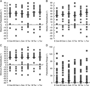
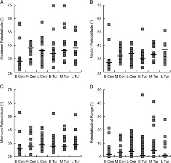
The majority of cephalopod occurrences in the database occur in northern midlatitudes, reflecting in part the large number of North American occurrences recorded in USGS records (Fig. 10). Considering all cephalopod genera together, the only significant differences in paleolatitudinal distribution through time are for the maximum (Fig. 10A, Table 5) and median (Fig. 10B, Table 6) paleolatitudes between the late Cenomanian and early Turonian (pairwise Mann-Whitney U-tests with Bonferroni and false discovery rate corrections, maximums=41.4° and 36.8°, medians=39.8° and 33.7°, p=0.0003 and 0.0002, respectively), showing a southward shift across the C/T boundary. On the other hand, no significant difference exists in minimum paleolatitudes (Fig. 10C) or paleolatitudinal range (Fig. 10D) among substages.
Global paleolatitudinal distributions of cephalopod genera through the Cenomanian–Turonian interval. Each square represents the median value of occurrences for one genus. Horizontal black bars mark the median value for each substage. A, Maximum paleolatitude. B, Median paleolatitude. C, Minimum paleolatitude. D, Paleolatitudinal range (i.e., maximum − minimum paleolatitude). Substage abbreviations as in Fig. 3. The only significant differences among substages are for the maximum and median paleolatitudes between the late Cenomanian and early Turonian, showing a southward shift across the C/T boundary (see Tables 5 and 6).

Results of Mann-Whitney U-tests comparing maximum paleolatitudes of cephalopod genera globally through time. Lower diagonal provides uncorrected p-values, while upper diagonal provides false discovery rate–corrected significance levels. Bonferroni-corrected significance level=0.0033. Significantly different pairs are in bold type. Cen, Cenomanian; Tur, Turonian.

Results of Mann-Whitney U-tests comparing median paleolatitudes of cephalopod genera globally through time. Lower diagonal provides uncorrected p-values, while upper diagonal provides false discovery rate–corrected significance levels. Bonferroni-corrected significance level=0.0033. Significantly different pairs are in bold type. Cen, Cenomanian; Tur, Turonian.

Considering each cephalopod superfamily separately, it is clear that the acanthoceratoids, which comprise 50% of genera and 60% of occurrences and species, are driving the observed paleolatitudinal pattern. They show a significant shift south across the C/T boundary in maximum (from 40.7°N to 34.1°N, p=0.0026; Table 7), median (from 37.1°N to 33.4°N, p=0.0000; Table 8), and minimum (from 33.3°N to 7.7°S, p=0.0023; Table 9) paleolatitudes. The overall paleolatitudinal range, however, does not change—this superfamily simply shifts south across the C/T boundary without contracting or expanding its latitudinal distribution.
Results of Mann-Whitney U-tests comparing maximum paleolatitudes of acanthoceratoid genera globally through time. Lower diagonal provides uncorrected p-values, while upper diagonal provides false discovery rate–corrected significance levels. Bonferroni-corrected significance level=0.0033. Significantly different pairs are in bold type. Cen, Cenomanian; Tur, Turonian.

Results of Mann-Whitney U-tests comparing median paleolatitudes of acanthoceratoid genera globally through time. Lower diagonal provides uncorrected p-values, while upper diagonal provides false discovery rate–corrected significance levels. Bonferroni-corrected significance level=0.0033. Significantly different pairs are in bold type. Cen, Cenomanian; Tur, Turonian.

Results of Mann-Whitney U-tests comparing minimum paleolatitudes of acanthoceratoid genera globally through time. Lower diagonal provides uncorrected p-values, while upper diagonal provides false discovery rate–corrected significance levels. Bonferroni-corrected significance level=0.0033. Significantly different pairs are in bold type. Cen, Cenomanian; Tur, Turonian.

The superfamily Turrilitoidea also shows several differences between substages in its median paleolatitude, which are significant using the false discovery rate correction but not the Bonferroni correction. Specifically, median paleolatitude shifts north from the early to the late Cenomanian (from 34.3°N to 40.8°N, p=0.0188; Table 10). Also, the median paleolatitudes of the middle Turonian are significantly more northern than those of the early and middle Cenomanian (46.5°N vs. 34.3°N and 36.6°N, p=0.0057 and 0.0138, respectively), whereas those of the late Turonian are significantly more northern than those of the middle Cenomanian (45.6°N vs. 36.6°N, p=0.0123). No significant differences through time in maximum paleolatitude, minimum paleolatitude, or paleolatitudinal range were found for Turrilitoidea.
Results of Mann-Whitney U-tests comparing median paleolatitudes of turrilitoid genera globally through time. Lower diagonal provides uncorrected p-values, while upper diagonal provides false discovery rate–corrected significance levels. Bonferroni-corrected significance level=0.0033. Significantly different pairs under false discovery rate correction (but not under Bonferroni correction) are in bold type. Cen, Cenomanian; Tur, Turonian.

No other cephalopod group shows any significant change in paleolatitudinal distribution throughout the C–T interval. Overall, it is notable that genera did not shift poleward during this time of global warming and decreased latitudinal temperature gradient.
Regional Latitudinal Distributions
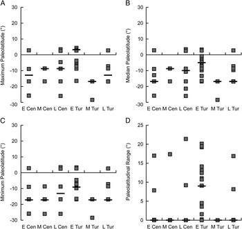
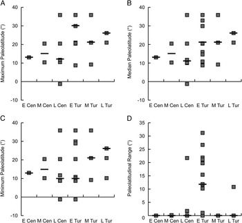
Paleolatitudinal distributions were also assessed separately for each of the identified biogeographic regions, with the exception of the Southern Ocean, which had insufficient data to conduct statistical testing. Distributions are shown in Figs. 11–15. Full results of each test are available in Supplementary Table 2.
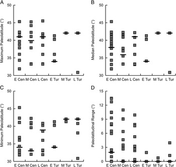
Paleolatitudinal distributions of cephalopod genera in the European Platform through the Cenomanian–Turonian interval. Each square represents the median value of occurrences for one genus. Horizontal black bars mark the median value for each substage. A, Maximum paleolatitude. B, Median paleolatitude. C, Minimum paleolatitude. D, Paleolatitudinal range (i.e., maximum − minimum paleolatitude). Substage abbreviations as in Fig. 3.

Paleolatitudinal distributions of cephalopod genera in the Western Interior Seaway through the Cenomanian–Turonian interval. Each square represents the median value of occurrences for one genus. Horizontal black bars mark the median value for each substage. A, Maximum paleolatitude. B, Median paleolatitude. C, Minimum paleolatitude. D, Paleolatitudinal range (i.e., maximum − minimum paleolatitude). Substage abbreviations as in Fig. 3.

Paleolatitudinal distributions of cephalopod genera in the South Atlantic through the Cenomanian–Turonian interval. Each square represents the median value of occurrences for one genus. Horizontal black bars mark the median value for each substage. A, Maximum paleolatitude. B, Median paleolatitude. C, Minimum paleolatitude. D, Paleolatitudinal range (i.e., maximum − minimum paleolatitude). Substage abbreviations as in Fig. 3.

Paleolatitudinal distributions of cephalopod genera in the Pacific through the Cenomanian–Turonian interval. Each square represents the median value of occurrences for one genus. Horizontal black bars mark the median value for each substage. A, Maximum paleolatitude. B, Median paleolatitude. C, Minimum paleolatitude. D, Paleolatitudinal range (i.e., maximum − minimum paleolatitude). Substage abbreviations as in Fig. 3.

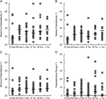
Paleolatitudinal distributions of cephalopod genera in Tethys through the Cenomanian–Turonian interval. Each square represents the median value of occurrences for one genus. Horizontal black bars mark the median value for each substage. A, Maximum paleolatitude. B, Median paleolatitude. C, Minimum paleolatitude. D, Paleolatitudinal range (i.e., maximum − minimum paleolatitude). Substage abbreviations as in Fig. 3.

Cephalopod distributions within the European Platform were generally stable through time (Fig. 11). Notably, however, maximum paleolatitude shifted significantly south toward the equator across the C/T boundary (40.8°N vs. 34.1°N, p=0.0067) before returning north in the middle and late Turonian. Median paleolatitude during the early Turonian was also significantly further south than in the late Turonian (34.1°N vs. 42.1°N, p=0.0013). Minimum paleolatitude did not show any significant differences through time, however, and paleolatitudinal ranges remained low throughout the C–T interval.
Within the WIS, the clearest difference is in the paleolatitudinal distributions of the early Cenomanian: maximum, median, and minimum paleolatitudes are significantly farther south than in all later substages (Fig. 12, Supplementary Table 2). This pattern makes sense, as the southern and northern portions of the WIS did not fully connect until the middle Cenomanian, so the majority of fossil occurrences in the early Cenomanian are from the southernmost portion of the seaway. Additionally, as in the European Platform, the maximum and median paleolatitudes shifted southward across the C/T boundary (41.1°N vs. 39.4°N, p=0.0134 and 39.5°N vs. 34.7°N, p=0.0146, respectively). Minimum paleolatitude, however, did not change significantly across the C/T, and paleolatitudinal range did not change within the WIS at any time during the C–T interval.
The South Atlantic region (Fig. 13) shows a similar shift equatorward (in this case, more northward) across the C/T boundary in maximum and median paleolatitudes, with the early Turonian values being significantly closer to the equator than for all other substages (Supplementary Table 2). Minimum paleolatitude during the early Turonian was also significantly more equatorward than the middle Cenomanian (−8.8°N vs. −16.8°N, p=0.0058) and middle Turonian (−8.8°N vs. −16.8°N, p=0.0000). Latitudinal range size in the early Turonian was significantly larger than during the late Turonian (9.1° vs. 0°, p=0.0036). Overall, the early Turonian stands out as an unusual time for cephalopod distributions in the South Atlantic.
Cephalopods from the Pacific (Fig. 14) and Tethyan (Fig. 15) regions, which include deeper-water settings, show almost no significant changes in any of the metrics of paleolatitudinal distribution. The only significant difference is a shift northward in median paleolatitude from the early to middle Cenomanian in the Pacific (46.7°N vs. 65.1°N, p=0.0028).
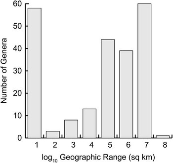
Geographic Ranges
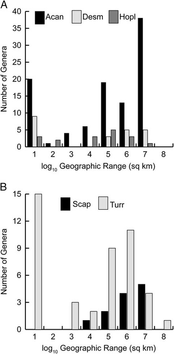
The majority of genera within each substage had small geographic ranges (Fig. 16). Although this pattern is partly due to genera known from single occurrences, the peak remains if singletons are excluded (as shown in Fig. 16), because many genera with small ranges are known from multiple localities in close proximity to one another. Considering the five most common ammonoid superfamilies (which comprise 94.1% of occurrences in the database) separately, several patterns emerge. Acanthoceratoidea includes many genera with large geographic ranges, in addition to a number of genera with very small ranges; fewer genera had intermediate range sizes (Fig. 17A). Desmoceratoidea also shows this gap at intermediate ranges but with relatively few genera with large ranges (Fig. 17A). That more acanthoceratoid than desmoceratoid genera had large ranges is surprising, as Acanthoceratoidea is dominated by shallow-water genera that could have been restricted to specific epicontinental basins, whereas Desmoceratoidea is characterized by many deep-water taxa that have been previously interpreted as having higher dispersal capabilities. Hoplitoidea shows a more bell-shaped distribution of geographic ranges, with a peak at intermediate range sizes (Fig. 17A). The two heteromorph genera show different geographic range distributions (Fig. 17B). Turrilitoidea’s distribution resembles that of Hoplitoidea, but with slightly larger ranges plus many genera with small ranges. Scaphitoidea, on the other hand, shows a unique pattern of mostly very large geographic ranges.
Geographic ranges of cephalopod genera within each substage of the Cenomanian–Turonian interval. Genera known from only a single locality have been excluded; if included, the number of genera in the leftmost bin jumps from 58 to 176. Note that geographic ranges of genera present in more than one substage are calculated separately for each substage, so a genus may be counted twice in the histogram.

Geographic ranges of cephalopod genera in five ammonoid superfamilies. A, Acanthoceratoidea, Desmoceratoidea, and Hoplitoidea. B, Scaphitoidea and Turrilitoidea. Genera known from only a single locality have been excluded; if included, the number of genera in the leftmost bin increases to 67 (Acan), 26 (Desm), 11 (Turr), 4 (Scap), and 35 (Turr). Taxon abbreviations as in Fig. 5.

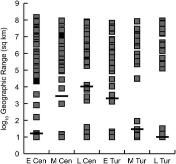
Although median geographic ranges of cephalopod genera increased through the Cenomanian before dropping in the Turonian (Fig. 18), these changes were not significant (pairwise Mann-Whitney U-tests with sequential Bonferroni correction all nonsignificant; Table 11). This result holds for all genera considered together and for superfamilies considered separately (Supplementary Table 2). Overall, therefore, cephalopod genera did not expand or contract their geographic ranges through this time of rising sea level or across the C/T boundary. It is notable, however, that intermediate geographic ranges disappear through the Turonian (Fig. 18).
Distributions of geographic range sizes of cephalopod genera through the Cenomanian–Turonian interval. Each square represents the geographic range for one genus. Horizontal black bars mark the median value for each substage. Number of genera in each time interval: E Cen=61, M Cen=52, L Cen=78, E Tur=64, M Tur=41, L Tur=47. Substage abbreviations as in Fig. 3.

Results of Mann-Whitney U-tests comparing global geographic range size of cephalopod genera through time. Lower diagonal provides uncorrected p-values, while upper diagonal provides false discovery rate–corrected significance levels. Bonferroni-corrected significance level=0.0033. Note no pairs are significantly different. Cen, Cenomanian; Tur, Turonian.

Restricted vs. Cosmopolitan Distributions
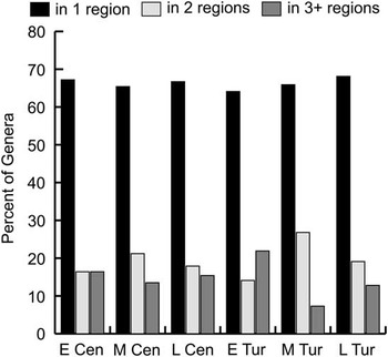
Cephalopod genera restricted to one biogeographic region predominate throughout the C–T interval, with the percentage of restricted genera in each substage varying only slightly from 64% to 68% during these times (Fig. 19). The percentage of genera found in two regions was relatively low in the early Cenomanian (16%) and early Turonian (14%) and higher in the middle Turonian (27%), with other substages showing intermediate values (Fig. 19). Cosmopolitan genera found in three or more regions show more variability through time, in particular a large increase across the C/T boundary from 15% in the late Cenomanian to 22% in the early Turonian (Fig. 19). The percentage of these widespread genera then dropped to just 7% in the middle Turonian before climbing again to 13% in the late Turonian.
Percentage of restricted vs. cosmopolitan cephalopod genera within each substage of the Cenomanian–Turonian interval. The majority of genera were restricted to a single region (black), whereas the percentage of genera occurring in two (light gray) or three or more (dark gray) of the six defined regions varied somewhat over time. Total numbers of genera included can be found in Table 3. Substage abbreviations as in Fig. 3.

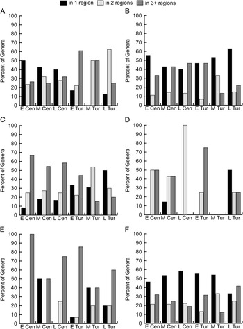
These global trends are also found within some but not all of the different biogeographic regions. In the European Platform, for example, the percentage of cephalopod genera restricted to that region dropped somewhat from a high of 50% in the early Cenomanian to 40% in the late Cenomanian, and then dropped much more across the C/T boundary to 17% in the early Turonian and a remarkable 0% in the middle Turonian (Fig. 19). Concomitant with the large drop in the restricted genera during the early Turonian was a large jump in cosmopolitan genera found in three or more regions, from 32% in the late Cenomanian to a high of 61% in the early Turonian (Fig. 20A). This decrease in restricted genera and increase in widespread genera across the C/T boundary mirrors the pattern seen in the global data, although the proportion of genera in the European Platform restricted to that region is lower than the global values.
Percentage of restricted vs. cosmopolitan cephalopod genera through time in each of six regions. A, European Platform. B, Pacific. C, South Atlantic. D, Southern Ocean. E, Tethys. F, Western Interior Seaway. Total numbers of genera included can be found in Table 3. Substage abbreviations as in Fig. 3.

In contrast, in the Pacific the percentage of restricted genera actually increased across the C/T boundary, from 40% to 47%, whereas the percentage of cosmopolitan genera stayed steady at 47% (Fig. 20B). Restricted genera were most common in the Pacific in the early Cenomanian (56%), middle Turonian (53%), and late Turonian (63%), whereas the proportion of cosmopolitan genera dropped in the middle Turonian (13%; Fig. 20B).
As in the Pacific, restricted genera found only in the South Atlantic increased from 17% in the late Cenomanian to 33% in the early Turonian, whereas cosmopolitan genera found in three or more regions decreased from 58% to 44% (Fig. 20C). Again, the middle Turonian appears to be a time of decreased widespread genera (15%), similar to the Pacific pattern but in contrast to the European Platform.
Available data for the Southern Ocean are limited, with just 0 to 8 genera present per substage, but it is notable that very few genera are restricted to this region, at least until the late Turonian, when 4 of the 8 genera present were found only in the Southern Ocean (Fig. 20D). The record from Tethys is also fairly slim, with 2 to 14 genera per substage. However, the number of cosmopolitan Tethyan genera present in three or more regions is notably high, including an increase from 75% to 86% across the C/T boundary (Fig. 20E).
The well-sampled WIS shows a high percentage of genera restricted to the WIS (ranging from 46% to 59% per substage, excluding the late Turonian; Fig. 20F). Restricted genera dropped just slightly across the C/T boundary, from 59% in the late Cenomanian to 55% in the early Turonian. The percentage of cosmopolitan genera found in three or more regions, conversely, jumped from 19% in the late Cenomanian to 32% in the early Turonian (Fig. 20F). These changes across the C/T boundary to a larger proportion of cosmopolitan genera mirror those seen in the European Platform and stand in contrast to those in the Pacific and South Atlantic. It should be noted, however, that the WIS showed relatively more restricted and fewer widespread genera than Europe, even in the early Turonian.
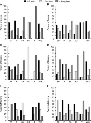
In addition to examining temporal patterns within each region, we can also consider how the six regions varied within each substage of the C–T interval (Fig. 21). During the early Cenomanian, the European Platform, Pacific, and WIS had a relatively high percentage of genera restricted to one region (i.e., more provincialism), whereas the South Atlantic, Southern Ocean, and Tethys had more cosmopolitan cephalopod genera (Fig. 21A). In the middle and late Cenomanian, the proportion of restricted genera decreased somewhat in the European Platform and Pacific, whereas the WIS remained the region with highest provincialism and the South Atlantic showed continuing cosmopolitanism (Fig. 21B, C). By the early Turonian, these patterns had changed. Cosmopolitan taxa dominated the European Platform, whereas the Pacific and South Atlantic both hosted a more even distribution of restricted versus cosmopolitan genera. The percentage of cosmopolitan taxa increased in the WIS at this time, although restricted genera continued to predominate (Fig. 21D). For the rest of the Turonian, the European Platform continued to host predominantly widespread genera, whereas the degree of provincialism increased in the Pacific and the South Atlantic (Fig. 21E,F). By the late Turonian, the Pacific, rather than the WIS, was the region with the highest percentage of restricted genera (Fig. 21F).
Percentage of restricted vs. cosmopolitan cephalopod genera by region within each substage of the Cenomanian–Turonian interval. A, Early Cenomanian. B, Middle Cenomanian. C, Late Cenomanian. D, Early Turonian. E, Middle Turonian. F, Late Turonian. EP, European Platform; P, Pacific; SA, South Atlantic; SO, Southern Ocean; T, Tethys; WIS, Western Interior Seaway. Total numbers of genera included can be found in Table 3.

Discussion
Globally, cephalopods do not show a significant drop in species- or genus-level diversity across the C/T boundary, which is consistent with the findings of Monnet (Reference Monnet2009). Instead, diversity lows occurred in the middle Cenomanian (as also reported by Monnet et al. Reference Monnet, Bucher, Escarguel and Guex2003; Monnet and Bucher Reference Monnet and Bucher2007b; Kurihara et al. Reference Kurihara, Toshimitsu and Hirano2012) and in the middle Turonian (Fig. 4). These diversity drops are associated with two times of brief cooling and rapid sea-level changes during overall greenhouse warming (Paul et al. Reference Paul, Mitchell, Marshall, Leary, Gale, Duane and Ditchfield1994; Hancock Reference Hancock2003; Miller et al. Reference Miller, Wright and Browning2005; Bice et al. Reference Bice, Birgel, Meyers, Dahl, Hinrichs and Norris2006; Forster et al. Reference Forster, Schouten, Baas and Sinninghe Damsté2007a; Giraud et al. Reference Giraud, Reboulet, Deconinck, Martinez, Carpentier and Bréziat2013), suggesting that cooler temperatures and/or rapid changes in environmental conditions may be critical controls for cephalopod diversity. The impact of the C/T event varied among ammonoid superfamilies, with some showing a drop in species and genera across the boundary (Turrilitoidea, Hoplitoidea, Tetragonitoidea), whereas others show an increase in species (Acanthoceratoidea, Scaphitoidea; Fig. 5). This clade-level variation in response to C/T environmental changes complicates the interpretation of causal processes driving cephalopod biodiversity.
Significant regional variations in cephalopod diversity change through the C–T interval are documented here, which may reflect differences in the degree and timing of environmental perturbations within different oceanographic settings. It is notable that the epicontinental WIS and open-ocean Pacific both show a diversity drop across the C/T boundary, whereas the epicontinental European Platform shows an increase (Figs. 8 and 9B,F vs. A). Given that the mixed-setting tropical South Atlantic and Tethys show peak diversity in the early Turonian (Figs. 8 and 9C,E), it may be that settings with greater cold-water influences (WIS, North Pacific) were more strongly affected by C/T warming. Previous work by Jagt-Yazykova (Reference Jagt-Yazykova2011, Reference Jagt-Yazykova2012), showing a diversity drop in cephalopods across the C/T boundary in the northwest Pacific, and Monnet (Reference Monnet2009), showing a diversity increase in Tunisia, is consistent with this pattern. A better understanding of the drivers of these regional cephalopod diversity differences will require careful documentation of regional variations in a variety of paleoceanographic proxies (such as stable isotopes, lithology, organic carbon content, and microfossil occurrences) for oxygen levels, temperatures, primary productivity, stratification, and sea level. While a few studies have emphasized regional differences in these parameters (e.g., Thomas and Tilghman Reference Thomas and Tilghman2014), most paleoceanographic studies through the C–T interval have focused on documenting globally correlatable patterns for the purposes of producing a robust global stratigraphic framework for OAE2. Differences in the regional response of cephalopods to perturbations through the C–T indicate that more focus on differences, rather than similarities, in the geologic record of environmental change among basins is warranted.
The expectation during a time of global warming is for taxa to shift or expand their latitudinal ranges poleward; however, cephalopod genera shifted maximum and median latitudes equatorward across the C/T boundary instead (Fig. 10). This global pattern is driven by the dominant ammonoid superfamily, Acanthoceratoidea; other superfamilies show no change across the C/T. Examining latitudinal changes within each of the six regions, the equatorward shift occurred in the European Platform (Fig. 11), WIS (Fig. 12), and South Atlantic (Fig. 13), whereas Pacific (Fig. 14) and Tethyan (Fig. 15) cephalopods did not change their latitudinal distributions. The latter two regions include deeper-water faunas that may have been more resistant to temperature-related oceanographic changes. However, it remains unclear why cephalopod distributions elsewhere would contract equatorward during this time of warming. One possibility is that cephalopods tracked the changing distribution of dysoxic waters associated with OAE2 rather than water temperatures across the C/T, perhaps in order to meet resting metabolic oxygen demand, as has been documented for modern marine ectotherms (Deutsch et al. Reference Deutsch, Ferrell, Seibel, Pörtner and Huey2015). A useful test of this idea would be to create a geospatial model of oceanographic conditions, including the changing spatial distribution of dysoxia and temperature through time, and map cephalopod occurrences onto it. A paleoceanographic model for the WIS is currently being developed, and future work will use this model to relate cephalopod distributions within the WIS to paleoceanographic parameters.
The two end-member models being tested here predict that geographic ranges would either increase or decrease in response to global warming; however, C–T cephalopods show no significant change in global geographic ranges through time at the genus level. It remains possible that constituent species’ ranges did indeed change without affecting genus-level ranges or that geographic distributions within individual basins or oceanographic settings changed. These options will be tested in a forthcoming paper. However, it seems clear that sea-level rise and warming did not produce a globally recognizable change in the geographic distribution of C–T cephalopods.
Generic geographic ranges did not change across the C/T boundary (Fig. 18, Table 11); however, the percentage of genera found in three or more regions did increase significantly before dropping in the middle Turonian (Fig. 19). This global pattern is mirrored in the records from the European Platform (Fig. 20A) and WIS (Fig. 20F), whereas the percentage of cosmopolitan genera dropped across the C/T in the Pacific (Fig. 20B) and South Atlantic (Fig. 20C). Several possible explanations exist for these differences in cosmopolitanism through time and space. It may be that during the late Cenomanian, endemic radiations within the WIS and European Platform produced an unusually high number of restricted taxa. The C/T event may then have shut down these “species factories.” Also, peak sea-level rise around the C/T may have allowed invaders to spread into formerly restricted basins, producing more cosmopolitan faunas in the early Turonian. It should be noted, however, that globally (Fig. 19), and especially in the WIS (Fig. 20F), the percentage of restricted genera remains relatively high throughout the C–T interval. The notion of epicontinental seaways as species factories is to be explored in a forthcoming paper.
Scaphitoidea shows a unique pattern of mostly very large geographic ranges (Fig. 17B). Scaphitoids from the latest Maastrichtian show a similarly large geographic spread (Landman et al. Reference Landman, Goolaerts, Jagt, Jagt-Yazykova, Machalski and Yacobucci2014). Scaphitoids first appeared in the Albian, and these results suggest that scaphitoid genera quickly established large geographic ranges, a feature that persisted throughout the Late Cretaceous. On the other hand, some evidence exists that scaphitoid species may have had more limited migration ability (Yahada and Wani Reference Yahada and Wani2013); hence the genus-level geographic distribution may differ from the species-level pattern.
Neither proposed end-member model for biodiversity change in a greenhouse world is supported for C–T cephalopods. Through the Cenomanian, cephalopod diversity increased substantially without an associated decrease in generic geographic range. Changes in diversity and degree of provincialism across the C/T varied by region and were not accompanied by changes in generic geographic range or a poleward latitudinal expansion. One interpretation of this pattern is that rising sea level and greenhouse warming led to both endemic radiations in epicontinental basins, driving biodiversity increase, and an increase in cosmopolitan taxa, such that median geographic ranges and latitudinal positions did not change significantly. Supporting this view is the strongly bimodal distribution of geographic ranges for the most diverse C–T cephalopod superfamily, Acanthoceratoidea (Fig. 17A). Others have previously argued that, during the C–T, a homogeneous cosmopolitan ammonoid fauna lived in outer shelf–open ocean habitats while repeatedly giving rise to rapidly radiating endemic faunas in adjacent epicontinental seas (e.g., Courville Reference Courville2007). This “why not both?” interpretation is also consistent with our understanding that ancient cephalopods showed a wide range of ecologies and modes of life (Ikeda and Wani Reference Ikeda and Wani2012; Ritterbush et al. Reference Ritterbush, Hoffmann, Lukeneder and De Baets2014), such that different genera may have responded differently to the global changes they faced through the Cenomanian and Turonian. In this context, it is also notable that ammonoid superfamilies generally considered to have been solely open-ocean dwellers (Phylloceratoidea, Desmoceratoidea) show little change in diversity or geographic distributions throughout the entire C–T interval.
Several outstanding issues remain to be investigated. Standing species and genus richness were tracked in this study, and it will be enlightening to calculate origination and extinction rates to more quantitatively assess the impact of C–T environmental change on origination and extinction probabilities and regional variations in turnover rates across the C/T boundary. An explanation is also needed for the unexpected C/T shift equatorward instead of poleward in cephalopod latitudinal distributions, and for the diversity lows in the middle Cenomanian and middle Turonian.
Sampling biases also need to be considered (Vilhena and Smith Reference Vilhena and Smith2013; Yang et al. Reference Yang, Ma and Kreft2013). For example, the European Platform is best sampled in the Cenomanian, whereas the Pacific, South Atlantic, and Tethys are best sampled in the early Turonian. How much does sampling influence the differences in diversity patterns seen in these regions? Comparisons with the more evenly sampled WIS may help separate real patterns from sampling biases. The South Atlantic shows substantial variations in sampling over time. Might the global latitudinal shift southward across the C/T boundary be due to oversampling in the hydrocarbon-rich early Turonian of West Africa, or is it a real pattern driven by cephalopods exploiting the Trans-Saharan Seaway, which first developed in the late Cenomanian–early Turonian, as a corridor from Tethys to the South Atlantic? Better sampling throughout the Southern Hemisphere and especially in the South Atlantic basin may help resolve this uncertainty.
Temporal and taxonomic resolution can also affect observed patterns. Monnet and Bucher (Reference Monnet and Bucher2007b) noted that when diversity studies use higher temporal resolution, sampling and stratigraphic biases may become more pronounced; they urged comparison of basinal, regional, and global patterns. Vilhena and Smith (Reference Vilhena and Smith2013) also argued that short-term diversity patterns are likely to be region specific. Hence, further subdivision of the regional data set into separate basins, with the potential for finer temporal resolution (to ammonoid zone or subzone), would be fruitful. The relationship between species-level geographic distributions and those of their encompassing genera could also be investigated (Foote et al. Reference Foote, Ritterbush and Miller2016). Are wide-ranging genera composed of wide-ranging species or of more geographically restricted species that happen to have arisen in multiple, separate basins around the world?
Different techniques for quantifying geographic distributions might also produce different results (Yang et al. Reference Yang, Ma and Kreft2013; Wu and Miller Reference Wu. and Miller2014). As an example, Miller et al. (Reference Miller, Aberhan, Buick, Bulinski, Ferguson, Hendy and Kiessling2009) found an unusual lack of a clear relationship between geographic distances between regions and marine faunal dissimilarity (geodisparity) for the Mesozoic versus the Paleozoic or Cenozoic. Wu and Miller (Reference Wu. and Miller2014) found that using overwater distance instead of great circle distance as the metric of geographic distance had an effect on the results for the Maastrichtian (their Cretaceous 8) but not for other intervals within the Mesozoic. As geographic information system approaches become more widespread in paleontology, more sophisticated ways of documenting geographic distributions and relating them to environmental and biodiversity changes are emerging (Stigall and Lieberman Reference Stigall and Lieberman2006; Myers et al. Reference Myers, Stigall and Lieberman2015). Such methods hold great promise for understanding biotic responses to the global changes experienced in the greenhouse world of the mid-Cretaceous.
Conclusions
-
∙ Two end-member models are proposed that relate greenhouse conditions to marine animal biodiversity dynamics. Global warming and increasing sea level might lead to: (1) increased dispersal, larger geographic ranges, and decreased speciation and biodiversity; or (2) increased endemism in epicontinental basins, smaller geographic ranges, and increased speciation and biodiversity. The models are tested for cephalopods during the C–T interval of the Late Cretaceous.
-
∙ Globally, neither species- nor genus-level diversity changed significantly across the C/T boundary. However, regional differences are documented, with diversity drops across the C/T boundary in the Pacific and the WIS of North America, slightly increased diversity in the European Platform, and peak diversity during the early Turonian in the South Atlantic and Tethys. These patterns may reflect the more negative impact of global warming on cephalopods occurring in basins that were more influenced by cold-water masses.
-
∙ Cephalopods in the European Platform, South Atlantic, and Western Interior shifted equatorward rather than poleward across the C/T boundary. This counterintuitive response to global warming may indicate that oxygen levels were a more important driver of cephalopod distributions than water temperature.
-
∙ While generic geographic ranges did not change significantly across the C/T boundary, the number of cosmopolitan genera increased in the European Platform and Western Interior and decreased in the Pacific and South Atlantic. The epicontinental seas of Europe and North America may have acted as endemic species factories during the Cenomanian that were shut down during the C/T crisis.
-
∙ Neither end-member model fits the patterns of cephalopod diversity and paleobiogeography during the C–T interval. Instead, global warming and sea-level rise may have both increased endemism in expanding epicontinental seaways and promoted long-distance dispersal among basins.
Acknowledgments
This study would not have been possible without the extraordinary efforts of my former student R. MacKenzie, who compiled a tremendous amount of data on Cretaceous cephalopod occurrences in North America for his 2007 M.S. thesis. His contributions are warmly acknowledged here. I also thank K. C. McKinney (USGS) for his input and advice about these data and A. Hendy (Natural History Museum, Los Angeles County) and other contributors to the PBDB for their work. Michael Foote and three anonymous reviewers provided many valuable suggestions for improving the paper, which are greatly appreciated. Finally, I thank T. Avruch for his suggestions and assistance.
Supplementary Material
Data available from the Dryad Digital Repository: http://dx.doi.org/10.5061/dryad.126dg