1 Introduction
Large-scale flows driven by a buoyancy gradient applied along a surface of constant gravitational potential play an important role in geophysics and in industrial applications. For example, the atmosphere of Venus absorbs most of the incoming solar radiation along its upper edge (Houghton Reference Houghton1977). Another example is found in the glass manufacturing industry. The temperature of the upper surface of a glass furnace is varied by the addition of cold floating raw materials at one end and heating by gas flames from above (Chiu-webster, Hinch & Lister Reference Chiu-webster, Hinch and Lister2008). Flows that are driven by this arrangement of boundary conditions are called horizontal convection (HC) flows (Stern Reference Stern1975).
HC flows are characterized by three non-dimensional parameters: the aspect ratio of the domain, the ratio of viscosity to diffusivity of the stratifying agent and the Rayleigh number, which measures the relative strength of the buoyancy forcing relative to viscous forces. Here we mostly focus on how HC changes as the Rayleigh number varies. Unlike the much more studied Rayleigh–Bénard convection, HC has attracted much less attention. Early experimental work led Sandström (Reference Sandström1908) to hypothesize, based on thermodynamic arguments, the existence of an asymptotic regime at high values of the Rayleigh number characterized by a shallow surface circulation. Later, Jeffreys (Reference Jeffreys1925) argued that for a surface-forced flow, thermodynamics requires only that the return flow of the dense fluid has to occur underneath the flow of light fluid (and vice versa for a bottom-forced flow). More recently, Paparella & Young (Reference Paparella and Young2002) provided a rigorous bound on the amount of kinetic energy dissipation that occurs within a horizontally convecting flow. This result, which became known as the ‘anti-turbulence’ theorem, calls into question whether HC can sustain turbulent flows at high values of the Rayleigh numbers. Whether a truly turbulent flow exists in HC has been the object of several studies (Scotti & White Reference Scotti and White2011; Stewart, Hughes & Griffiths Reference Stewart, Hughes and Griffiths2011; Gayen et al. Reference Gayen, Griffiths, Hughes and Saenz2013; Griffiths, Hughes & Gayen Reference Griffiths, Hughes and Gayen2013), which together show that for values of the Rayleigh number greater than a critical value, HC flows are characterized by turbulent regions and extremely efficient mixing.
Recently, Gayen, Griffiths & Hughes (Reference Gayen, Griffiths and Hughes2014) investigated the successive flow transitions in horizontal convection using direct numerical simulations and reported the existence of several flow structures which control the transition to turbulence. At high Rayleigh numbers, the flow is not simply characterized by a single overturning cell. Instead the heavy sinking fluid immediately reflects upon hitting the lower boundary, and the fluid in the core of the domain mixes while forming large-scale steady structures. In the transverse direction, the flow appeared to be strongly dominated by steady convection rolls, as well as convective instabilities, transporting a large amount of turbulent kinetic energy in the recirculating core.
The stability of HC flows, and how it relates to the flow transitions observed by Gayen et al. (Reference Gayen, Griffiths and Hughes2014) and others, has been very recently investigated using a local stability analysis of the parallel base flow (Tsai et al.
Reference Tsai, Hussam, Fouras and Sheard2016) or in the radially rotating case combining local and global stability analyses (Sheard, Hussam & Tsai Reference Sheard, Hussam and Tsai2016). Combining a local and a global stability analysis will help clarify the mechanisms responsible for flow transition, turbulence and mixing. It may also shed light on whether a deep circulation is maintained at high
 $Ra$
or whether the flow eventually transition to the regime hypothesized by Sandström.
The instability characteristics and thresholds are expected to be sensitive to the value of the Prandtl number (Shishkina & Wagner Reference Shishkina and Wagner2016), though the effect of the Prandtl number on the instability dynamics is beyond the scope of this paper.
Combining the results from the stability analysis with the available potential energy analysis of Scotti & White (Reference Scotti and White2014) will allow us to assess the role of each individual mode determining mixing efficiency. It can also provide guidelines for the receptivity and the control of mixing in horizontal convection (Marquet, Sipp & Jacquin Reference Marquet, Sipp and Jacquin2008; Foures, Caulfield & Schmid Reference Foures, Caulfield and Schmid2014). For instance surface stresses are known to play an important role in the mixing process (Beardsley & Festa Reference Beardsley and Festa1972; Whitehead & Wang Reference Whitehead and Wang2008; Tailleux & Rouleau Reference Tailleux and Rouleau2010; Hazewinkel, Paparella & Young Reference Hazewinkel, Paparella and Young2012; Ilicak & Vallis Reference Ilicak and Vallis2012) by substantially modifying the flow structure, and the circulation can be sensitive to enhanced rates of interior mixing (Stewart, Graham & Griffiths Reference Stewart, Graham and Griffiths2012).
The present work consists of local and global stability analyses (Edwards et al. Reference Edwards, Tuckerman, Friesner and Sorensen1994; Chomaz Reference Chomaz2005; Garnaud et al. Reference Garnaud, Lesshafft, Schmid and Chomaz2012) using two-dimensional steady states solved using direct numerical simulations, detailed in § 2. Results for the free-slip boundary conditions are presented in § 3 for the steady states and the stability analyses are detailed in § 4. The effect of no-slip boundary conditions on the flow is examined in § 5 and the consequences on the stability in § 6. These results show that two instabilities are competing. The sinking plume region is shown to be unstable to both a three-dimensional Rayleigh–Taylor (R–T) instability and a two-dimensional sheared Rayleigh–Taylor instability. The different critical Rayleigh numbers defining thresholds for instabilities are also reported together with the effect of the domain’s aspect ratio on the stability § 7. Conclusions are finally drawn in § 8.
The investigation of how the transition to turbulence and the turbulent flow characteristics are related to a subcritical bifurcation, will be discussed in a forthcoming paper.
2 Theoretical framework
2.1 Problem set-up
The fluid is assumed to be contained in a rectangular domain of aspect ratio
 $A\equiv L_{x}/H$
, where
 $H$
is the height and
 $L_{x}$
the length (
 $L_{y}$
will denote the width in the three-dimensional case). Using
 $H$
as a unit of length, the non-dimensional two-dimensional domain is
 $[-A/2,A/2]\times [0,1]$
. Here, similar to previous studies (Paparella & Young Reference Paparella and Young2002; Scotti & White Reference Scotti and White2011)
 $A=4$
will be used as a baseline geometry.
The flow is described by the incompressible Navier–Stokes equations in the Boussinesq limit with a linear equation of state. Under these assumptions, the density
 $\unicode[STIX]{x1D70C}$
is given by
 $\unicode[STIX]{x1D70C}=\unicode[STIX]{x1D70C}_{0}(1+\unicode[STIX]{x1D6FC}T)$
, where
 $T$
is the quantity that describes the stratifying agent and
 $\unicode[STIX]{x1D70C}_{0}$
is a reference density. In experiments involving water, stratification is normally controlled either via changes in temperature, in which case
 $\unicode[STIX]{x1D6FC}$
is the (negative) coefficient of thermal expansion (Niemela et al.
Reference Niemela, Skrbek, Sreenivasan and Donnelly2000; Roche et al.
Reference Roche, Castaing, Chabaud and Hébral2002; Mullarney, Griffiths & Hughes Reference Mullarney, Griffiths and Hughes2004), or via varying the concentration of a salt (Stewart et al.
Reference Stewart, Graham and Griffiths2012; Passaggia et al.
Reference Passaggia, Hurley, Scotti and White2017), and
 $\unicode[STIX]{x1D6FC}$
is the positive haline contraction coefficient. Since, from a theoretical point of view, the precise nature of the stratifying agent is irrelevant, we describe stratification in terms of the buoyancy
 $b\equiv g(\unicode[STIX]{x1D70C}_{0}-\unicode[STIX]{x1D70C})/\unicode[STIX]{x1D70C}_{0}$
, where
 $g$
is the acceleration of gravity.
 $b$
satisfies the same advection–diffusion equation of the stratifying agent. Let
 $\unicode[STIX]{x0394}b$
be the buoyancy contrast imposed by the boundary conditions. We can define a velocity scale
 $\sqrt{\unicode[STIX]{x0394}bH}$
, which allows to write non-dimensionalize the governing equations as follows
 $$\begin{eqnarray}\displaystyle \frac{\unicode[STIX]{x2202}\boldsymbol{u}}{\unicode[STIX]{x2202}t}+(\boldsymbol{u}\boldsymbol{\cdot }\unicode[STIX]{x1D735})\boldsymbol{u} & = & \displaystyle -\unicode[STIX]{x1D735}p+b\boldsymbol{e}_{\boldsymbol{z}}+\left(\frac{A^{3}Pr}{Ra}\right)^{1/2}\unicode[STIX]{x1D6FB}^{2}\boldsymbol{u},\end{eqnarray}$$
 $$\begin{eqnarray}\displaystyle \unicode[STIX]{x1D735}\boldsymbol{\cdot }\boldsymbol{u} & = & \displaystyle 0,\end{eqnarray}$$
 $$\begin{eqnarray}\displaystyle \frac{\unicode[STIX]{x2202}b}{\unicode[STIX]{x2202}t}+(\boldsymbol{u}\boldsymbol{\cdot }\unicode[STIX]{x1D735})b & = & \displaystyle \left(\frac{A^{3}}{Pr\,Ra}\right)^{1/2}\unicode[STIX]{x1D6FB}^{2}b,\end{eqnarray}$$
 $\boldsymbol{u}=(u,v,w)^{\text{T}}$
and
 $p$
are the non-dimensional velocity vector and pressure. The Rayleigh number is defined by
 $Ra=\unicode[STIX]{x0394}bL^{3}/(\unicode[STIX]{x1D708}\unicode[STIX]{x1D705})$
and the Prandtl number is given by
 $Pr=\unicode[STIX]{x1D708}/\unicode[STIX]{x1D705}$
where
 $\unicode[STIX]{x1D708}$
is the kinematic viscosity and
 $\unicode[STIX]{x1D705}$
is the diffusivity of the stratifying agent (calling
 $\unicode[STIX]{x1D708}/\unicode[STIX]{x1D705}$
the Prandtl number should not be construed as implying that we are thinking of heat as the stratifying agent). A value of
 $Pr=1$
was used throughout the present study. While it would be more realistic to use higher values, it would limit the range of Rayleigh numbers attainable. The unit vector
 $\boldsymbol{e}_{\boldsymbol{z}}$
points opposite the local gravity.
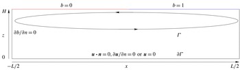
Sketch of the flow set-up.

The base flow is assumed to be two-dimensional whereas the perturbation is sought to be periodic in the transverse direction
 $y$
. The bottom and the side walls are insulating whereas a piecewise constant buoyancy profile
 $B(x<0,1)=0$
and
 $B(x>0,1)=1$
is imposed at the upper boundary (
 $z=1$
), as shown in figure 1. The choice of such idealized boundary conditions for the buoyancy was essentially motivated by previous studies (Gayen et al.
Reference Gayen, Griffiths, Hughes and Saenz2013, Reference Gayen, Griffiths and Hughes2014). The step profile here compared for instance to the linear profile provides more circulation as the amount of buoyancy provided for the circulation is larger for the step case than the linear case. More importantly, a step profile does not add an extra length scale to the problem, simplifying the analysis.
We consider both free- and no-slip boundary conditions for the velocity along the boundaries. The latter is required to model actual laboratory experiments, whereas the former is more appropriate if the aim is to extrapolate the results to geophysical situations, where no-slip boundary layers should play a negligible role. In the literature we find examples of both (Paparella & Young Reference Paparella and Young2002; Scotti & White Reference Scotti and White2011; Gayen et al.
Reference Gayen, Griffiths and Hughes2014). The flow domain was discretized with
 $400$
points using fourth-order finite differences for the Laplacian and eighth-order differences for the gradient in the longitudinal direction and
 $60$
Chebyshev collocation points in the vertical direction.
2.2 Steady states method
Steady solutions and the associated global stability results were obtained across the range
 $6.4\times 10^{6}\leqslant Ra\leqslant 1.28\times 10^{10}$
for free-slip boundary conditions and
 $6.4\times 10^{6}\leqslant Ra\leqslant 1.28\times 10^{9}$
for the no-slip case. The choice was made to use a time stepper approach to compute both the steady states and the eigenvalue problem associated with the stability. The same procedure was used in Marquillie & Ehrenstein (Reference Marquillie and Ehrenstein2003) and Passaggia, Meunier & Le Dizès (Reference Passaggia, Meunier and Le Dizès2014) and details about the numerical methods can be found in Marquillie & Ehrenstein (Reference Marquillie and Ehrenstein2002). Equilibrium states, steady solutions of the system (2.1), are computed using the selective frequency damping method (Akervik et al.
Reference Akervik, Brandt, Henningson, Hœpffner, Marxen and Schlatter2006)
 $$\begin{eqnarray}\left.\begin{array}{@{}l@{}}\displaystyle \unicode[STIX]{x2202}_{t}\boldsymbol{q}=\boldsymbol{F}(\boldsymbol{q},Re)-\unicode[STIX]{x1D701}(\boldsymbol{q}-\bar{\boldsymbol{q}}),\\ \displaystyle \unicode[STIX]{x2202}_{t}\bar{\boldsymbol{q}}=\frac{1}{\unicode[STIX]{x1D6EC}}(\boldsymbol{q}-\bar{\boldsymbol{q}}),\end{array}\right\}\end{eqnarray}$$
where
 $\boldsymbol{q}=(\boldsymbol{u},p,b)^{\text{T}}$
. For the stabilization coefficients, the optimal cutoff frequency
 $\unicode[STIX]{x1D6EC}=12.7423$
and damping factor
 $\unicode[STIX]{x1D701}=0.0534$
computed at
 $Ra=1.28\times 10^{9}$
for the no-slip case were used to converge to a steady state (Cunha, Passaggia & Lazareff Reference Cunha, Passaggia and Lazareff2015). Simulations of system (2.1) were considered to be converged to a steady state when the
 $l_{2}$
-norm of the difference of the velocity and buoyancy fields renormalized with the time step, was smaller than
 $10^{-8}$
. Here the time step
 $\unicode[STIX]{x0394}t=2\times 10^{-3}$
was used for all the simulations and the forthcoming stability analysis.
2.3 Global instability modes
The flow solution
 $\boldsymbol{q}$
is decomposed into a steady state
 $\boldsymbol{Q}=(\boldsymbol{U},P,B)$
, and a perturbation with the special form
 $\boldsymbol{q}^{\prime }=(\boldsymbol{u}^{\prime }(x,z,t),p^{\prime }(x,z,t),b^{\prime }(x,z,t))\exp (\text{i}\unicode[STIX]{x1D6FD}y)$
. The linearized perturbation dynamics is governed by
 $$\begin{eqnarray}\displaystyle \frac{\unicode[STIX]{x2202}\boldsymbol{u}^{\prime }}{\unicode[STIX]{x2202}t}+(\boldsymbol{U}\boldsymbol{\cdot }\tilde{\unicode[STIX]{x1D735}})\boldsymbol{u}^{\prime }+(\tilde{\unicode[STIX]{x1D735}}\boldsymbol{U})\boldsymbol{u}^{\prime } & = & \displaystyle -\tilde{\unicode[STIX]{x1D735}}p^{\prime }+b^{\prime }\boldsymbol{e}_{\boldsymbol{ z}}+\left(\frac{A^{3}Pr}{Ra}\right)^{1/2}\tilde{\unicode[STIX]{x1D6FB}}^{2}\boldsymbol{u}^{\prime },\end{eqnarray}$$
 $$\begin{eqnarray}\displaystyle \tilde{\unicode[STIX]{x1D735}}\boldsymbol{\cdot }\boldsymbol{u}^{\prime } & = & \displaystyle 0,\end{eqnarray}$$
 $$\begin{eqnarray}\displaystyle \frac{\unicode[STIX]{x2202}b^{\prime }}{\unicode[STIX]{x2202}t}+(\boldsymbol{U}\boldsymbol{\cdot }\tilde{\unicode[STIX]{x1D735}})b^{\prime }+(\tilde{\unicode[STIX]{x1D735}}B)\boldsymbol{u}^{\prime } & = & \displaystyle \left(\frac{A^{3}}{Pr\,Ra}\right)^{1/2}\tilde{\unicode[STIX]{x1D6FB}}^{2}b^{\prime },\end{eqnarray}$$
 $\tilde{\unicode[STIX]{x1D735}}=(\unicode[STIX]{x2202}/\unicode[STIX]{x2202}x,\text{i}\unicode[STIX]{x1D6FD},\unicode[STIX]{x2202}/\unicode[STIX]{x2202}z)^{\text{T}}$
and
 $\tilde{\unicode[STIX]{x1D6FB}}^{2}=(\unicode[STIX]{x2202}^{2}/\unicode[STIX]{x2202}x^{2}-\unicode[STIX]{x1D6FD}^{2}+\unicode[STIX]{x2202}^{2}/\unicode[STIX]{x2202}z^{2})$
. The free-slip and no-slip boundary conditions for the velocity of the perturbation were considered. A Dirichlet condition
 $b^{\prime }=0$
was used at the upper boundary whereas the buoyancy perturbation is insulated in the rest of the domain. Note that the numerical methods and discretization are the same as described in § 2.2. The linear system (2.3) may be equivalently written
 $$\begin{eqnarray}\boldsymbol{E}\frac{\text{d}\boldsymbol{q}^{\prime }}{\text{d}t}=\unicode[STIX]{x1D63C}\boldsymbol{q}^{\prime },\end{eqnarray}$$
where
 $\unicode[STIX]{x1D63C}$
depends on
 $(\boldsymbol{U},\boldsymbol{B},Ra,Pr,\unicode[STIX]{x1D6FD})$
and
 $\boldsymbol{E}$
is the projection operator onto the velocity and buoyancy field such that
 $\boldsymbol{E}\boldsymbol{q}=(\boldsymbol{u},0,b)^{\text{T}}$
. The stability is computed by considering the three-dimensional temporal modes
 $\hat{\boldsymbol{q}}(x,z)\exp (-\text{i}(\unicode[STIX]{x1D714}t-\unicode[STIX]{x1D6FD}y))$
, where
 $\hat{\boldsymbol{q}}$
and
 $\unicode[STIX]{x1D714}$
satisfy the generalized eigenvalue problem
 $$\begin{eqnarray}-\text{i}\unicode[STIX]{x1D714}\boldsymbol{E}\hat{\boldsymbol{q}}=\unicode[STIX]{x1D63C}\hat{\boldsymbol{q}}.\end{eqnarray}$$
Here, the matrix
 $\unicode[STIX]{x1D63C}$
is not computed explicitly and it is advantageous for large eigenvalue problems to only consider the operator that takes a state
 $\boldsymbol{q}^{\prime }(t)$
as initial condition for (2.4) and returns to the state
 $\boldsymbol{q}^{\prime }(t+\unicode[STIX]{x0394}t)$
after a given time
 $\unicode[STIX]{x0394}t$
(Edwards et al.
Reference Edwards, Tuckerman, Friesner and Sorensen1994). Since Krylov-based eigenvalue solvers only require the storage of several flow states
 $\boldsymbol{q}^{\prime }(t)$
, the standard time marching algorithm is used to propagate the solution. However, such an approach will only identify a subset of eigenmodes with the largest growth rates
 $\unicode[STIX]{x1D714}_{i}$
. To circumvent this limitation, the generalized eigenvalue problem (2.5) was solved using the shift-and-relax method of Garnaud et al. (Reference Garnaud, Lesshafft, Schmid and Chomaz2012). The linear perturbation dynamics (2.4) was coupled to a lowpass filter
 $\bar{\boldsymbol{q}}$
such that
 $$\begin{eqnarray}\left.\begin{array}{@{}l@{}}\displaystyle \boldsymbol{E}\frac{\text{d}\boldsymbol{q}^{\prime }}{\text{d}t}=\unicode[STIX]{x1D63C}\boldsymbol{q}^{\prime }-\unicode[STIX]{x1D712}(\boldsymbol{q}^{\prime }-\bar{\boldsymbol{q}}),\\ \displaystyle \boldsymbol{E}\frac{\text{d}\bar{\boldsymbol{q}}}{\text{d}t}=-\text{i}\unicode[STIX]{x1D714}_{0}\bar{\boldsymbol{q}}-\unicode[STIX]{x1D70F}(\bar{\boldsymbol{q}}-\boldsymbol{q}^{\prime }).\end{array}\right\}\end{eqnarray}$$
This method allows for computing eigenmodes with different frequency ranges, such that real frequencies
 $\unicode[STIX]{x1D714}_{r}$
, far from the target frequency
 $\unicode[STIX]{x1D714}_{0,r}$
are attenuated (Garnaud et al.
Reference Garnaud, Lesshafft, Schmid and Chomaz2012). The parameters for the shift-and-relax method were
 $\unicode[STIX]{x1D712}=\unicode[STIX]{x1D70F}=0.1$
and all the computed eigenvalues were checked to converge with a relative precision of
 $10^{-3}$
, which is the bound given by the accuracy of the temporal scheme. Note that the system (2.6) is a generalization of (2.2) where the linear perturbation dynamics is forced at a particular frequency
 $\unicode[STIX]{x1D714}_{0}$
and damped everywhere else in the spectrum. The eigenvalues
 $\unicode[STIX]{x1D6FA}$
, associated with (2.6) can be transformed back to their original counterparts
 $\unicode[STIX]{x1D714}$
in (2.5) using the transformation (Garnaud et al.
Reference Garnaud, Lesshafft, Schmid and Chomaz2012)
 $$\begin{eqnarray}\unicode[STIX]{x1D714}(\unicode[STIX]{x1D6FA})=\unicode[STIX]{x1D6FA}+\text{i}\unicode[STIX]{x1D712}\left(1-\frac{1}{\displaystyle 1-\text{i}\frac{\unicode[STIX]{x1D6FA}-\unicode[STIX]{x1D714}_{0}}{\unicode[STIX]{x1D70F}}}\right).\end{eqnarray}$$
The eigenvalue problem is solved using a Krylov subspace of
 $80$
snapshots. Another simulation is also performed with a shift in the complex plane at
 $\unicode[STIX]{x1D714}_{0}=1$
to ensure the convergence of all the eigenvalues. All eigenvalues were computed with a relative error below
 $10^{-3}$
for each eigenvalue.
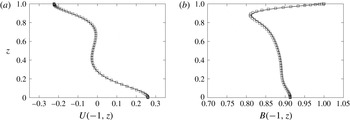
Comparison between the local vertical profiles for the three-dimensional DNS code (——) (Scotti Reference Scotti2008) computed in a narrow domain (i.e.
 $W=0.125$
) and the present two-dimensional DNS (
 $\Box$
) at
 $x=1$
and
 $Ra=2\times 10^{6}$
and
 $A=4$
for the horizontal velocity
 $U(z)$
(a) and the buoyancy
 $B(z)$
(b), in the free-slip case.

2.4 Validation of the numerical procedure
Results have been compared with a separate, well-validated, three-dimensional DNS code Scotti (Reference Scotti2008), and profiles of buoyancy and velocity were found to differ by less than 1 % between the two codes (e.g. see figure 2
a,b). The fact that the local and global stability analyses provide comparable results offers a validation of the stability analysis procedure. Also, verification of the bi-orthogonality condition (see (6.1) introduced in § 6.2) proves that the stability codes were implemented correctly. Furthermore, the local stability results offer a cross-validation for the stability methods used in the present study. We also simulated the flow using a three-dimensional DNS code for a transverse box width
 $W=1$
at
 $Ra=2\times 10^{6}$
in the free-slip case, and recovered the three-dimensional instability predicted by the stability analyses. The same code was also used and validated in previous studies (Marquillie & Ehrenstein Reference Marquillie and Ehrenstein2002, Reference Marquillie and Ehrenstein2003; Passaggia, Leweke & Ehrenstein Reference Passaggia, Leweke and Ehrenstein2012; Passaggia et al.
Reference Passaggia, Meunier and Le Dizès2014; Cunha et al.
Reference Cunha, Passaggia and Lazareff2015). Further detail on validation of the codes used here may be found therein.
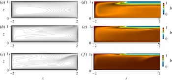
Streamlines (a–c) and buoyancy distribution (d–f) of the steady base flows at
 $Ra=1.92\times 10^{7}$
(a,d),
 $Ra=1.44\times 10^{8}$
(b,e) and
 $Ra=6.4\times 10^{8}$
(c,f) at
 $Pr=1$
,
 $A=4$
using free-slip boundary conditions.

3 Free-slip steady states
For sufficiently small Rayleigh numbers and an aspect ratio
 $A=4$
, the two-dimensional flow solution is stable and the selective frequency damping coefficient is set to
 $\unicode[STIX]{x1D701}=0$
. The problem is thus marched in time to converge to a steady state which is achieved at
 $t\approx 1000$
. For instance, at
 $Ra=1.44\times 10^{8}$
the flow is characterized by a single counterclockwise rotating cell spanning the entire domain, and a small clockwise rotating cell, located under a less dense layer of fluid, near the surface in the top right corner (cf. figure 3
a,d). Increasing further the Rayleigh number, the perturbation dynamics becomes progressively less stable and the selective frequency damping method was coupled starting at
 $Ra=3.2\times 10^{9}$
to allow convergence to a steady state. Increasing the Rayleigh number also increases the complexity of the flow and the main recirculation cell exhibits a complex structure with the onset of co-rotating vortices, essentially located in the lower part of the domain, under the stable fluid layer. This is shown in figure 3(c,f) at
 $Ra=6.4\times 10^{8}$
where the upwelling reflects on the stable layer and either returns directly back to the heavy layer, or remains trapped in the small co-rotating cells located at the centre of the domain. For this larger value of the Rayleigh number, the size of the clockwise rotating cell is also smaller and confined in the corner.
4 Stability analysis
The basic flow in horizontal convection generates an unstable density profile beneath the surface where
 $b=0$
is imposed, which approaches the plume region as a narrow jet (cf. figure 3). In this region, the fluid is subject to the destabilizing effect of the boundary condition (
 $b=0$
) imposed at the top and shear within the jet. As a result, this gravitationally unstable region can be expected to excite Rayleigh–Taylor type instabilities. The e-folding time scale of R–T instabilities is (Chandrasekhar Reference Chandrasekhar1961)
 $$\begin{eqnarray}T_{RT}\sim \left(\frac{\unicode[STIX]{x1D708}}{\unicode[STIX]{x0394}b^{2}}\right)^{1/3}.\end{eqnarray}$$
Here
 $\unicode[STIX]{x0394}b$
is the buoyancy difference across the layer, assumed to be very close to the buoyancy difference imposed by the boundary conditions. The viscous diffusion time across a layer of thickness
 $\unicode[STIX]{x1D6FF}$
is
 $$\begin{eqnarray}T_{\unicode[STIX]{x1D708}}\sim \unicode[STIX]{x1D6FF}^{2}/\unicode[STIX]{x1D708}.\end{eqnarray}$$
Assuming a scaling for the thickness
 $\unicode[STIX]{x1D6FF}$
of the jet
 $$\begin{eqnarray}\frac{\unicode[STIX]{x1D6FF}}{H}\sim Ra^{-\unicode[STIX]{x1D6FE}},\end{eqnarray}$$
we have (Hazewinkel et al. Reference Hazewinkel, Paparella and Young2012)
 $$\begin{eqnarray}\frac{T_{RT}}{T_{\unicode[STIX]{x1D708}}}\sim Ra^{-2/3+2\unicode[STIX]{x1D6FE}}.\end{eqnarray}$$
In the present low-Rayleigh number regime, the flow characteristics follow the Rossby scaling
 $\unicode[STIX]{x1D6FE}=1/5$
(Rossby Reference Rossby1965). Thus for increasing values of
 $Ra$
, diffusion cannot smooth out the unstable density contrast and the R–T instability is expected to become active. In the following sections, we show that the flow is subject to two different types of instabilities. The steady flow initially becomes unstable with respect to a three-dimensional instability, which is characterized by transverse counter-rotating rolls localized in the plume region, defined by the wavenumber
 $\unicode[STIX]{x1D6FD}$
associated with the direction
 $y$
. The second instability, discussed in § 6.1, sets in at a higher
 $Ra$
, is enhanced by the presence of the no-slip boundary conditions, is two-dimensional and is associated with a sheared Rayleigh–Taylor instability located in the thin jet, in the unstable layer. This instability exhibits a wave-like structure with
 $\unicode[STIX]{x1D6FC}$
the wavenumber in the longitudinal direction
 $x$
.
4.1 Three-dimensional global modes
The DNS results of Gayen et al. (Reference Gayen, Griffiths and Hughes2014) suggest that the most amplified global modes are three-dimensional and are characterized by steady counter-rotating vortices with axes aligned along the
 $x$
direction. These modes have been observed for a large range of Rayleigh numbers and mark the onset of instability in horizontal convection. To study these modes, a global stability analysis was performed over a range of Rayleigh numbers
 $Ra=[2.02,2.56]\times 10^{7}$
and transverse wavenumbers
 $\unicode[STIX]{x1D6FD}=[4,8]$
where a family of unstable modes was found. These modes are characterized by zero frequency, meaning that they are steady with growth rates in the range
 $\unicode[STIX]{x1D714}_{i}=[-8.6\times 10^{-3},1.194\times 10^{-2}]$
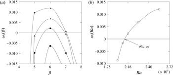
. These growth rates are shown in figure 4(a) as a function of the transverse wavenumber
 $\unicode[STIX]{x1D6FD}$
. Increasing the Rayleigh number appears to increase both the growth rate and the most unstable wavenumber, as well as the unstable wavenumber range. The critical Rayleigh number for this mode was found at
 $Ra_{c,3D}\approx 1.24\times 10^{8}$
and gives the onset of instability for an aspect ratio
 $A=4$
(cf. figure 4
b).
Growth rate
 $\unicode[STIX]{x1D714}_{i}$
(a) of the most unstable three-dimensional global mode as a function of the transverse wavenumber
 $\unicode[STIX]{x1D6FD}$
at
 $Ra=2\times 10^{7}$
(-▪-),
 $Ra=2.08\times 10^{7}$
(-●-),
 $Ra=2.24\times 10^{7}$
(-▴-),
 $Ra=2.56\times 10^{7}$
(-▾-). Most unstable growth rate
 $\unicode[STIX]{x1D714}_{i}$
(b) as a function of the Rayleigh number
 $Ra$
, depicting also the critical Rayleigh number
 $Ra_{c,3D}=2.02\times 10^{7}$
at
 $A=4$
, for free-slip boundary conditions.

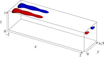
Visualization of the most unstable three-dimensional eigenmode by means of iso-buoyancy surfaces
 $\hat{b}=\pm 44\,\%$
normalized by the maximum of
 $\hat{b}$
(red/blue) at
 $Ra=1.44\times 10^{8}$
,
 $Pr=1$
,
 $\unicode[STIX]{x1D6FD}=6$
and
 $\unicode[STIX]{x1D714}_{i}=0.0026259$
, for free-slip boundary conditions.

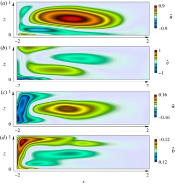
Velocity distribution
 $\hat{u} (x,z)$
(a),
 $\hat{v}(x,z)$
(b),
 ${\hat{w}}(x,z)$
(c),
 $\hat{b}(x,z)$
(d), of the most unstable three-dimensional mode (
 $\unicode[STIX]{x1D6FD}=6$
) at
 $Ra=1.44\times 10^{8}$
and
 $Pr=1$
, using free-slip boundary conditions (the amplitude was normalized using the maximum of transverse velocity
 $\hat{v}$
).

The structure of the unstable modes, shown in figure 5, is characterized by convection rolls, originating in the vicinity of the statically unstable fluid in the upper left boundary. In the near-surface region, the global instability mode, shown in figure 5, is essentially characterized by an increase of buoyancy and longitudinal vorticity. Within the descending plume, all quantities appear to switch sign (cf. figure 6). The same observation can be made near the bottom of the domain where the counter-rotating vortices span most of the lower boundary. Finally, its structure vanishes in the upwelling region.
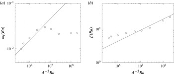
The growth rates and the most unstable wavenumber for larger values of the Rayleigh number are shown in figure 7(a,b). The growth rate follows the inverse scaling of the e-folding time scale given in (4.1), suggesting that the instability is of the Rayleigh–Taylor type. This scaling however changes at
 $Ra\approx 6.4\times 10^{8}$
and this interesting feature will be discussed in a forthcoming manuscript. The scaling for the most unstable wavelength follows a
 $Ra^{1/3}$
for all values of
 $Ra$
, confirming the hypothesis of a Rayleigh–Taylor instability.
Most unstable growth rate
 $\unicode[STIX]{x1D714}_{i}$
(a) as a function of
 $Ra$
(○) compared with the
 $Ra^{2/3}$
scaling (——). Most unstable wavenumber
 $\unicode[STIX]{x1D6FD}$
(b) as a function of
 $Ra$
(○) compared with the
 $Ra^{1/3}$
scaling (——), using free-slip boundary conditions.

4.1.1 Local stability criteria
A sufficient criterion for Rayleigh–Taylor instability in an inviscid stratified fluid can be sought in terms of the Richardson number
 $$\begin{eqnarray}Ri=\frac{N^{2}}{\displaystyle \left(\frac{\unicode[STIX]{x2202}U}{\unicode[STIX]{x2202}z}\right)^{2}},\end{eqnarray}$$
which quantifies locally the ratio between the buoyancy forces to the shear and where the Brunt–Väisälä frequency is given in our units by
 $N^{2}=\unicode[STIX]{x2202}b/\unicode[STIX]{x2202}z$
. For
 $0\leqslant Ri<1/4$
, one expects shear driven type instabilities to dominate whereas
 $Ri<0$
correspond to regions of statically unstable fluid, with the potential for Rayleigh–Taylor instability (see for instance Dolzhansky (Reference Dolzhansky2012) for a derivation). If there exists a streamline
 $\unicode[STIX]{x1D713}_{0}$
such that for all the points
 $r_{0}$
belonging to the streamline, the local Richardson number is below
 $0$
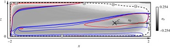
, we expect Rayleigh–Taylor instabilities. Circled points are drawn on the streamline depicted in figure 8, labelled
 $i=0,5,\ldots ,60$
such that the absolute time values at these points are
 $t_{i}=i$
when following a particle on its trajectory. Here
 $C$
locates the centre for the streamlines of the main recirculation region, where all particle trajectories are initialized. This gives an idea of the velocity intensity along the streamline. There exist different regions of the flow where the Richardson number is negative: a strongly negative region under the boundary of statically unstable fluid, the plume, and weaker regions along the bottom and in the upwelling. There is no closed streamline along which the local Richardson number remains below
 $1/4$
nor
 $0$
. However, particles following closed streamlines inside the recirculation zone travel every period through regions where they are exposed to convectively unstable conditions. Keeping in mind that
 $Ri<0$
is only a sufficient condition for instability, the aim of § 4.1.2 is to analyse if this partial gain is sufficient to trigger the global instability revealed in § 4.1 by our global mode analysis.
Iso-values of the growth rate predicted by the Wentzel–Kramers–Brillouin analysis along streamlines are represented in grey levels (i.e. white is the most amplified streamline) at
 $Ra=1.44\times 10^{8}$
, using free-slip boundary conditions. The most unstable streamline is represented by a black dashed line. Iso-contours of the Richardson number
 $Ri$
are also shown, for values ranging from
 $1/4$
to
 $0.01$
(blue dashed line). The transition from positive to negative values
 $Ri=0$
is shown by the continuous line in red whereas negative values ranging from
 $0$
to
 $-15$
are shown by the red dashed lines.

4.1.2 Wentzel–Kramers–Brillouin (WKB) method along streamlines
In the so-called geometric optics method (or WKB method), the perturbation velocity and pressure are sought in the form of wave packets
 $$\begin{eqnarray}[\boldsymbol{u},p,b]=[\boldsymbol{a}(t),c(t),d(t)]\text{e}^{\text{i}\boldsymbol{k}(t)\boldsymbol{x}(t)}.\end{eqnarray}$$
Following Bayly (Reference Bayly1988), Majda & Shefter (Reference Majda and Shefter1998) and Gallaire, Marquillie & Ehrenstein (Reference Gallaire, Marquillie and Ehrenstein2007), the growth rate associated with any closed streamline in the limit of zero viscosity and large wavenumber
 $\boldsymbol{k}$
is found by integrating the following set of equations
 $$\begin{eqnarray}\displaystyle \frac{\text{d}\boldsymbol{x}}{\text{d}t} & = & \displaystyle \boldsymbol{U}(\boldsymbol{x}(t)),\end{eqnarray}$$
 $$\begin{eqnarray}\displaystyle \frac{\text{d}\boldsymbol{k}}{\text{d}t} & = & \displaystyle -\unicode[STIX]{x1D647}^{\text{T}}(\boldsymbol{x}(t))\boldsymbol{k},\end{eqnarray}$$
 $$\begin{eqnarray}\displaystyle \frac{\text{d}\boldsymbol{a}}{\text{d}t} & = & \displaystyle \left(\frac{2\boldsymbol{k}(t)\boldsymbol{k}^{\text{T}}(t)}{|\boldsymbol{k}(t)|^{2}}-\boldsymbol{I}\right)\unicode[STIX]{x1D647}(\boldsymbol{x}(t))\boldsymbol{a}-\left(\frac{k_{z}}{|\boldsymbol{k}|^{2}}\boldsymbol{k}-\boldsymbol{e}_{z}\right)d(t),\end{eqnarray}$$
 $$\begin{eqnarray}\displaystyle \frac{\text{d}d}{\text{d}t} & = & \displaystyle \unicode[STIX]{x1D735}B\boldsymbol{\cdot }(\boldsymbol{x}(t))\boldsymbol{a}(t),\end{eqnarray}$$
 $\unicode[STIX]{x1D647}(x(t))$
is the velocity-gradient matrix
 $\unicode[STIX]{x1D735}\boldsymbol{U}$
at position
 $x(t)$
attained at time
 $t$
. The first equation simply restates that the (two-dimensional) position of the particle along the trajectory
 $x(t)$
remains tangent to the velocity vector
 $\boldsymbol{U}(x(t))$
. The second, third and fourth equations describe respectively the evolution of the three-dimensional wavenumber
 $\boldsymbol{k}(t)$
and the perturbation amplitude
 $[\boldsymbol{a}(t),d(t)]$
along the streamline as time evolves. Four initial conditions should be added
 $$\begin{eqnarray}\boldsymbol{x}(t=0)=\boldsymbol{x}_{0},\quad \boldsymbol{k}(t=0)=\boldsymbol{k}_{0},\quad \boldsymbol{a}(t=0)=\boldsymbol{a}_{0},\quad d(t=0)=d_{0},\end{eqnarray}$$
where the first condition imposes the Lagrangian origin
 $\boldsymbol{x}_{0}$
of the streamline and thereby entirely identifies the streamline. Since the second column of
 $\unicode[STIX]{x1D647}$
and thereby the second line of
 $\unicode[STIX]{x1D647}^{\text{T}}$
are zero, the transverse component
 $k_{y}=\unicode[STIX]{x1D6FD}$
of
 $\boldsymbol{k}$
is independent of time. In contrast, the in-plane components evolve under the action of the deformation tensor. Bayly (Reference Bayly1988), Lifschitz & Hameiri (Reference Lifschitz and Hameiri1991) and Sipp & Jacquin (Reference Sipp and Jacquin1998) have shown that other types of instabilities like the centrifugal and the hyperbolic instabilities do attain their maximum growth rate for purely transverse wavenumbers. These instability modes are also called pressureless modes (see Hunt & Vassilicos Reference Hunt and Vassilicos2011, p. 251) since pressure is essentially independent of the
 $x$
and
 $z$
components. The same remark applies in the present analysis where the shape of the mode is not determined by the pressure induced by gradients in the
 $x$
and
 $z$
directions (cf. figure 6), but rather by the transverse wavelike structure, where
 $\unicode[STIX]{x1D6FD}\gg 1/L$
. The structure found in § 4.1 by the global mode analysis suggests the following ansatz
 $\boldsymbol{k}_{0}=\unicode[STIX]{x1D6FD}_{0}\boldsymbol{e}_{y}$
, yielding
 $\boldsymbol{k}(t)=\unicode[STIX]{x1D6FD}_{0}\boldsymbol{e}_{y}$
. With this assumption, equation (4.7) becomes
 $$\begin{eqnarray}\displaystyle \frac{\text{d}\boldsymbol{a}}{\text{d}t} & = & \displaystyle \tilde{\unicode[STIX]{x1D647}}(\boldsymbol{x}(t))\boldsymbol{a}+\boldsymbol{e}_{z}d(t),\end{eqnarray}$$
 $$\begin{eqnarray}\displaystyle \frac{\text{d}d}{\text{d}t} & = & \displaystyle -\unicode[STIX]{x1D735}B\boldsymbol{\cdot }(\boldsymbol{x}(t))\boldsymbol{a}(t),\end{eqnarray}$$
 $$\begin{eqnarray}\tilde{\unicode[STIX]{x1D647}}=\left(\begin{array}{@{}ccc@{}}-1 & 0 & 0\\ 0 & 1 & 0\\ 0 & 0 & -1\end{array}\right)\unicode[STIX]{x1D647}.\end{eqnarray}$$
As a consequence of the periodic nature of the flow along closed streamlines, the coupled system (4.9) is studied using Floquet theory over one period
 $T(x_{0})$
solving
 $$\begin{eqnarray}\frac{\text{d}\unicode[STIX]{x1D63C}}{\text{d}t}=\tilde{\unicode[STIX]{x1D648}}(\boldsymbol{x}(t))\unicode[STIX]{x1D63C},\quad \text{with}~\unicode[STIX]{x1D63C}(t=0)=\boldsymbol{I},\end{eqnarray}$$
and where
 $$\begin{eqnarray}\tilde{\unicode[STIX]{x1D648}}=\left(\begin{array}{@{}cccc@{}}\displaystyle -\frac{\unicode[STIX]{x2202}U}{\unicode[STIX]{x2202}x}(\boldsymbol{x}(t)) & 0 & \displaystyle -\frac{\unicode[STIX]{x2202}U}{\unicode[STIX]{x2202}z}(\boldsymbol{x}(t)) & 0\\ 0 & 0 & 0 & 0\\ \displaystyle -\frac{\unicode[STIX]{x2202}W}{\unicode[STIX]{x2202}x}(\boldsymbol{x}(t)) & 0 & \displaystyle -\frac{\unicode[STIX]{x2202}W}{\unicode[STIX]{x2202}z}(\boldsymbol{x}(t)) & -1\\ \displaystyle -\frac{\unicode[STIX]{x2202}B}{\unicode[STIX]{x2202}x}(\boldsymbol{x}(t)) & 0 & \displaystyle -\frac{\unicode[STIX]{x2202}B}{\unicode[STIX]{x2202}z}(\boldsymbol{x}(t)) & 0\end{array}\right).\end{eqnarray}$$
The growth rate is then obtained by calculating the Floquet exponents associated with the eigenvalues
 $\unicode[STIX]{x1D706}_{1,\ldots ,4}(x_{0})$
, and associated eigenvectors
 $\hat{\boldsymbol{a}}_{1,\ldots ,4}(x_{0})$
, of the
 $4\times 4$
matrix
 $\unicode[STIX]{x1D63C}(T(x_{0}))$
. Note that in regions where the flow is parallel (i.e.
 $\unicode[STIX]{x2202}_{x}U\approx \unicode[STIX]{x2202}_{x}B\approx 0$
) the two non-zero eigenvalues of
 $\unicode[STIX]{x1D648}$
are
 $\pm \sqrt{N^{2}(\boldsymbol{x}(t))}$
. In this limit, equation (4.9) readily leads to
 $\unicode[STIX]{x1D706}_{2,3,4}=1$
and
 $a_{2,3,4}=e_{2,3,4}$
.
The maximum growth rate is then evaluated by considering the real part of
 $$\begin{eqnarray}\unicode[STIX]{x1D70E}_{1}(x_{0})=\log (\unicode[STIX]{x1D706}_{1}(x_{0}))/T(x_{0}),\end{eqnarray}$$
where
 $T(x_{0})$
is the time necessary to complete a closed path along a streamline. Note that for any Lagrangian origin
 $\boldsymbol{x}_{0}$
belonging to the streamline
 $\unicode[STIX]{x1D713}_{0}$
,
 $\unicode[STIX]{x1D70E}_{1}(\boldsymbol{x}_{0})\equiv \unicode[STIX]{x1D70E}_{1}(\unicode[STIX]{x1D713}_{0})$
.
Equation (4.9) together with (4.7a
) are integrated via a fourth-order Runge–Kutta method for Lagrangian origins on several streamlines. The interpolation scheme used here to interpolate the velocity of the Eulerian grid on to the particle position was performed using a standard bi-linear scheme. The corresponding real and imaginary parts of
 $\unicode[STIX]{x1D70E}_{1}(\unicode[STIX]{x1D713}_{0})$
are reported in figure 9 where each streamline
 $\unicode[STIX]{x1D713}_{0}$
is labelled by the ordinate
 $x_{0}$
of the intersection point with the arrow depicted in figure 8, parallel to the
 $x$
-axis from the centre
 $C=(0.962,0.425)$
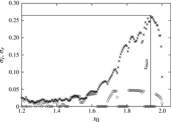
to the right wall. As a complement, the intensity of the growth rate associated with each closed streamline is also reported in figure 8 using a grey scale. The maximum growth rate is real (i.e. the frequency of the eigenvalue
 $\text{Im}(\unicode[STIX]{x1D70E})=0$
), in agreement with the numerical simulation and global instability analysis, and it is obtained for the streamline shown in figure 8 and corresponding to
 $x_{0}=x_{max}=1.935$
in figure 9.
The results of the WKB analysis show that a positive growth rate is expected, with a maximum located in the gravitationally unstable region. These results are qualitatively consistent with the R–T instability mechanism. However, the growth rate predicted by the large wavenumber asymptotic limit
 $\unicode[STIX]{x1D6FD}\rightarrow \infty$
and
 $Ra\rightarrow \infty$
(
 $\unicode[STIX]{x1D70E}_{\infty }\approx 0.25$
) is not in quantitative agreement with the growth rate measured in the global mode analysis at
 $Ra=1.44\times 10^{8}$
and
 $\unicode[STIX]{x1D6FD}=6=O(10)$
(
 $\unicode[STIX]{x1D70E}\approx 3.27\times 10^{-4}$
) (see figure 5). While the WKB method is inherently inviscid, in reality, the growth rate is determined by a complex balance of transient growth and transient viscous damping. In the next section, we introduce a viscous damping term and finite-
 $\unicode[STIX]{x1D6FD}$
terms into the evolution equation and show that accounting for these effects allows the growth rate to be accurately reproduced.
Growth rate
 $\unicode[STIX]{x1D70E}_{i}$
(
 $\ast$
) and frequency
 $\unicode[STIX]{x1D70E}_{r}$
(○) of the Wentzel–Kramers–Brillouin mode as a function of the streamline labelled by the abscissa
 $x_{0}$
along the arrow represented in figure 8.

4.1.3 Construction of the global mode
In the previous subsection we have shown that the inviscid WKB analysis at large wavenumber shows a stationary instability which is in qualitative agreement with the global mode analysis, but does not quantitatively reproduce the growth rates. Landman & Saffman (Reference Landman and Saffman1987) and Majda & Shefter (Reference Majda and Shefter1998) have discussed how to reintroduce viscosity. Formally, equations similar to (4.7) starting from the Navier–Stokes and not the Euler equations can be derived. Equations (4.7a,b ) remain unchanged and (4.7c,d ) should be replaced by
 $$\begin{eqnarray}\displaystyle & \displaystyle \frac{\text{d}\boldsymbol{a}}{\text{d}t}=\left(\tilde{\unicode[STIX]{x1D647}}(\boldsymbol{x}(t))-\unicode[STIX]{x1D6FD}^{2}\sqrt{A^{3}\frac{Pr}{Ra}}\right)\boldsymbol{a}+\boldsymbol{e}_{z}d(t), & \displaystyle\end{eqnarray}$$
 $$\begin{eqnarray}\displaystyle & \displaystyle \frac{\text{d}d}{\text{d}t}=\left(\unicode[STIX]{x1D735}B(\boldsymbol{x}(t))-\frac{A^{3/2}\unicode[STIX]{x1D6FD}^{2}}{\sqrt{PrRa}}\right)\boldsymbol{\cdot }\boldsymbol{a}(t) & \displaystyle\end{eqnarray}$$
In the present case we consider
 $Pr=1$
and the viscous corrected growth rate becomes
 $$\begin{eqnarray}\unicode[STIX]{x1D70E}_{vis}=\unicode[STIX]{x1D70E}_{\infty }-\frac{A^{3/2}\unicode[STIX]{x1D6FD}^{2}}{\sqrt{Ra}}\end{eqnarray}$$
Bayly (Reference Bayly1988) and Sipp & Jacquin (Reference Sipp and Jacquin1998) have demonstrated that it is possible to build an inviscid global mode of finite wavenumber
 $\unicode[STIX]{x1D6FD}$
in the vicinity of the most unstable streamline
 $\unicode[STIX]{x1D713}_{max}$
if a necessary condition for instability holds. Bayly (Reference Bayly1988) derived an asymptotic resolution of the boundary layer equations concentrated around
 $\unicode[STIX]{x1D713}_{max}$
. The first-order correction term including finite-
 $\unicode[STIX]{x1D6FD}$
effects is a term of the order of
 $-a/\unicode[STIX]{x1D6FD}$
, where
 $a$
is a constant, accounting for the asymptotically small spreading of the unstable mode. This is also confirmed graphically in figure 9 where the growth rate takes a quadratic maximum at
 $\unicode[STIX]{x1D70E}_{\infty }$
(see Bayly (Reference Bayly1988) and Sipp & Jacquin (Reference Sipp and Jacquin1998) for details). A similar correction term can only be inferred here (as done for instance by Sipp, Lauga & Jacquin (Reference Sipp, Lauga and Jacquin1999), regarding hyperbolic, centrifugal and even elliptic instabilities (Griffith et al.
Reference Griffith, Thompson, Leweke, Hourigan and Anderson2007)). Following the procedure of Gallaire et al. (Reference Gallaire, Marquillie and Ehrenstein2007) we have the following composite estimation
 $$\begin{eqnarray}\unicode[STIX]{x1D70E}_{vis}=\unicode[STIX]{x1D70E}_{\infty }-\frac{a}{\unicode[STIX]{x1D6FD}}-\frac{A^{3/2}\unicode[STIX]{x1D6FD}^{2}}{\sqrt{Ra}},\end{eqnarray}$$
which strictly makes sense only if
 $a^{2}A^{-3}Ra=O(\unicode[STIX]{x1D6FD}^{6})$
(i.e. the viscous correction and the boundary layer type term are of the same order). This way of reasoning neglects the influence of the viscosity in the mode structure, (i.e. one expects
 $a$
not to depend on
 $Ra$
). Equation (4.17) may now be used to derive scaling laws for the maximum growth rate
 $\unicode[STIX]{x1D70E}_{max}$
and wavenumber
 $\unicode[STIX]{x1D6FD}_{max}$
such that
 $$\begin{eqnarray}\displaystyle & \displaystyle \unicode[STIX]{x1D6FD}_{max}=\left(\frac{a^{2}A^{-3}Ra}{4}\right)^{1/6}, & \displaystyle\end{eqnarray}$$
 $$\begin{eqnarray}\displaystyle & \displaystyle \unicode[STIX]{x1D70E}_{max}=\unicode[STIX]{x1D70E}_{\infty }-(2^{1/3}+2^{-2/3})\left(\frac{a^{4}}{A^{-3}Ra}\right)^{1/6}. & \displaystyle\end{eqnarray}$$
It is interesting to note that at
 $\unicode[STIX]{x1D6FD}_{max}$
, the viscous correction and finite
 $\unicode[STIX]{x1D6FD}$
terms are of the same order, guaranteeing that
 $a^{2}A^{-3}Ra=O(\unicode[STIX]{x1D6FD}^{6})$
, thereby justifying the composite estimation (4.17). The scaling laws (4.18) and (4.19) can be compared against the results of the global stability analysis of § 4.1. The global stability analysis allows for decoupling the Rayleigh number determining the steady base flow topology from the Rayleigh number controlling the perturbation evolution, as required in the aforementioned theory. Five numerical experiments were conducted where the Rayleigh number was changed in the stability equations (but not in the base state computed at
 $1.44\times 10^{8}$
) at
 $Ra=[1.44\times 10^{8},6.4\times 10^{8},3.2\times 10^{9},1.28\times 10^{10},6.4\times 10^{11}]$
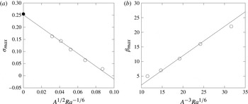
, in a similar way to § 4.1. The corresponding maximal numerical growth rates are reported in figure 10(a) as a function of
 $Ra^{-1/6}$
. The five test cases scale with the corrected growth rate
 $\unicode[STIX]{x1D70E}=\unicode[STIX]{x1D70E}_{0}-\unicode[STIX]{x1D70E}_{1}Ra^{-1/6}$
where
 $\unicode[STIX]{x1D70E}_{0}\approx 0.25$
, very close to
 $\unicode[STIX]{x1D70E}_{\infty }\approx 0.254$
. The scaling law (4.18) also well describes
 $\unicode[STIX]{x1D6FD}_{max}$
(figure 10
b). The quality of the collapse suggests that
 $A$
does not depend on
 $Ra$
, giving some support to the hypothesis that viscous corrections in the construction of the eigenmode may be neglected. We conclude that the geometric optics method designed for short wave inviscid instabilities, once suitably amended by viscous and finite wavenumber correction terms, provides a quantitatively accurate estimate of the growth rate and the wavelength at the origin of the three-dimensional Rayleigh–Taylor instability.
Maximum growth rate
 $\unicode[STIX]{x1D70E}$
(○) as computed from the global stability analysis at various Rayleigh numbers as a function of
 $Ra^{-1/6}$
, using free-slip boundary conditions. The inviscid asymptotic growth rate
 $\unicode[STIX]{x1D70E}_{\infty }$
is also shown (●). Wavenumber
 $\unicode[STIX]{x1D6FD}_{max}$
(○) at maximal growth rate (b) as a function of
 $Ra^{1/6}$
.

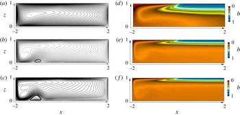
Streamlines (a–c) and buoyancy distribution (d–f) of the steady base flows at
 $Ra=6.4\times 10^{6}$
(a,d),
 $Ra=1.92\times 10^{8}$
(b,e) and
 $Ra=6.4\times 10^{8}$
(c,f) at
 $Pr=1$
,
 $A=4$
and no-slip boundary conditions.

5 No-slip boundary conditions
In the present buoyancy driven flow, the use of no-slip boundary conditions is expected to play an important role on the circulation due to modification of the base flow and therefore the unstable dynamics. As viscous boundary layers are reintroduced, the viscous dissipation induced by the boundary layers is expected to weaken the circulation for the small Rayleigh number regime presently investigated. This is shown in figure 11(a,d) at
 $Ra=6.4\times 10^{6}$
where the streamlines and the buoyancy distribution show a qualitative agreement compared with the base flows obtained for free-slip boundary conditions at the wall computed at
 $Ra=1.92\times 10^{7}$
. Increasing the Rayleigh number to
 $Ra=1.92\times 10^{8}$
the streamlines become very different and the two base flows show a very different topology where the plume is now partially confined under the unstable boundary and between the left wall and a counter rotating recirculation bubble, as shown in figure 11(b,e).
The modifications between the no-slip base flow and the free-slip one are characterized by:
-
(i) a slower circulation (weaker streamfunction),
-
(ii) a broader upwelling region,
-
(iii) the counter-rotating recirculation cell located at the base of the plume,
-
(iv) a thicker stratified layer,
-
(v) a rebound of the plume, remaining confined near the left wall.
Similarly to the free-slip case, the two-dimensional flow solution is stable for
 $Ra<6.4\times 10^{7}$
and the selective frequency damping coefficient is set to
 $\unicode[STIX]{x1D701}=0$
. However in the present case, increasing the Rayleigh number at
 $Ra=1.92\times 10^{8}$
resulted in a self-sustained unstable flow and the base flow could not be recovered, even for very long time of integration. The selective frequency damping method was coupled starting at
 $Ra=1.92\times 10^{8}$
to allow convergence to a steady state (Cunha et al.
Reference Cunha, Passaggia and Lazareff2015). This stabilizing procedure was carried out until
 $Ra=1.28\times 10^{9}$
where the damping coefficient
 $\unicode[STIX]{x1D701}$
was increased up to
 $0.1068$
and
 $\unicode[STIX]{x1D6EC}=25.48$
in order to allow the flow to converge to a steady state.
The increase of kinetic energy dissipation induced by the boundary layers at the wall appears to be responsible for the rebound of the plume. Interestingly, this observation seems to be also associated with the onset of the instabilities. This phenomena is reinforced as the Rayleigh number increases up to
 $Ra=6.4\times 10^{8}$
(cf. figure 11
c–f) and the counter-rotating recirculation region also increases, both in length and in height and the plume starts to describe closed streamlines near the bottom and the top of the domain.
In the no-slip regime, the vertical gradients of buoyancy are weaker compared with the free-slip solutions. In addition, the presence of boundary layers at the wall due to the no-slip boundary condition induce an interaction between the shear and the unstable stratification, which is expected to play a dominant role in the instability dynamics.
6 Two-dimensional global modes
As discussed in § 5, further increasing the Rayleigh number causes the base flow to become unstable with respect to two-dimensional perturbations. The perturbation takes the form of vortices originating in the heavy fluid at the base of the plume that are alternately shed along the base of the domain. The mechanism responsible for vortex shedding may either be related to the amplifier or the resonating nature of the flow. In the case of an amplifier, the flow is globally stable but the shear induced by the base flow may be sufficient to allow the growth of small amplitude perturbations and prevent the convergence of the flow back to a steady state. Instead, the resonator dynamics is described by self-sustained motion, due for instance to a region of absolute instability (Chomaz Reference Chomaz2005) or a feedback mechanism controlled by the non-parallel effects of the flow (Marquillie & Ehrenstein Reference Marquillie and Ehrenstein2003; Ehrenstein & Gallaire Reference Ehrenstein and Gallaire2008). Based on their DNS, Gayen et al. (Reference Gayen, Griffiths, Hughes and Saenz2013, Reference Gayen, Griffiths and Hughes2014) point out that this instability sets the transition to turbulence and plays an important role in the mixing process.
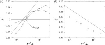
Growth rate
 $\unicode[STIX]{x1D714}_{i}$
as a function of
 $Ra$
at
 $Pr=1$
and
 $A=4$
of the most unstable two-dimensional eigenmode
 $\unicode[STIX]{x1D6FD}=0$
(○) and the most unstable three-dimensional mode (▫) (a), using no-slip boundary conditions. The solid line shows the scaling:
 $\text{Cst.}+0.2/5\log (A^{-3}Ra)$
. Most unstable frequency
 $\unicode[STIX]{x1D714}_{r}$
(▫) (b), associated with the growth rate shown in (a) for the same parameters. Here the solid line shows the scaling:
 $\text{Cst}.-0.4/30\log (A^{-3}Ra)$
.

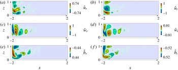
Velocity distribution (real–imaginary parts)
 $\hat{u} _{i,r}(x,z)$
(a,b),
 ${\hat{w}}_{i,r}(x,z)$
(c,d),
 $\hat{b}_{i,r}(x,z)$
(e,f) of the most unstable two-dimensional mode (
 $\unicode[STIX]{x1D6FD}=0$
), at
 $Ra=1.92\times 10^{8}$
and
 $Pr=1$
, using no-slip boundary conditions. (The amplitude was normalized using the maximum velocity
 $\hat{u} _{r}$
for the real part and
 ${\hat{w}}_{i}$
for the imaginary part.)

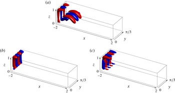
Visualization of the three-dimensional unstable eigenmodes by means of iso-buoyancy surfaces
 $\hat{b}=\pm 44\,\%$
(a) and
 $\hat{b}=\pm 10\,\%$
(b,c), normalized by the maximum of
 $\hat{b}$
(red/blue), at
 $Ra=6.4\times 10^{8}$
,
 $Pr=1$
,
 $\unicode[STIX]{x1D6FD}=9$
and
 $\unicode[STIX]{x1D714}=0.009185i$
(a) and
 $\unicode[STIX]{x1D6FD}=12$
and
 $\unicode[STIX]{x1D714}=0.0356i\pm 0.2304$
(b,c), using no-slip boundary conditions.

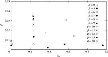
Global spectrum for each individual unstable mode for several transverse wavelengths at
 $Ra=6.4\times 10^{8}$
and
 $Pr=1$
, in the range
 $\unicode[STIX]{x1D6FD}=$
[0, 3, 6, 7, 8, 9, 10, 11, 12, 15, 20], using no-slip boundary conditions.

6.1 Global stability analysis
The growth rate of the pure two-dimensional mode (
 $\unicode[STIX]{x1D6FD}=0$
) is shown in figure 12(a) as a function of the Rayleigh number. The critical value for the onset of two-dimensional instability is found to be
 $Ra_{c,2D}\approx 1.65\times 10^{8}$
. The eigenfunction for the unstable two-dimensional mode (
 $\unicode[STIX]{x1D6FD}=0$
) is depicted in figure 13. The structure of the mode mostly spans the left boundary of the flow and takes the form of regular transverse vortices shed inside the domain, which effectively transport buoyancy as well as kinetic and potential energy. While the eigenfunction shown in figure 13 is for
 $\unicode[STIX]{x1D6FD}=0$
, pure Rayleigh–Taylor modes are found in the global spectrum for
 $\unicode[STIX]{x1D6FD}=9$
corresponding to transverse wavelengths smaller than the depth of the domain. Three-dimensional modes (cf. figure 14
b,c) are also found with a frequency and have a maximum growth rate
 $\unicode[STIX]{x1D714}_{i}$
, found for
 $\unicode[STIX]{x1D6FD}\sim 12$
. This is depicted in figure 15 where the global spectrum at
 $Ra=6.4\times 10^{8}$
is shown for several values of the transverse wavenumber. These modes also exhibit a lower frequency
 $\unicode[STIX]{x1D714}_{r}$
than the two-dimensional instability, and the latter seems to be independent of the Rayleigh number (cf. figure 12(b) showing the most unstable quasi two-dimensional mode at
 $Ra=6.4\times 10^{8}$
). Tsai et al. (Reference Tsai, Hussam, Fouras and Sheard2016) found similar results in their local stability analyses. They showed that both two and three-dimensional instabilities had comparable temporal growth rates using a local stability analysis of the parallel base flow near the plume.
They also computed the marginal stability and showed that the longitudinal and transverse rolls were marginally unstable at
 $Ra\approx 1.23\times 10^{7}$
but for
 $Pr=6.14$
and
 $A=6.25$
. The most unstable wavelength are also in qualitative agreements with the present study. Tsai et al. (Reference Tsai, Hussam, Fouras and Sheard2016) found that the onset of three-dimensional local instability was found near the plume, for
 $\unicode[STIX]{x1D6FD}\approx 19$
(in our units) compared to
 $\unicode[STIX]{x1D6FD}\approx 12$
in our global stability analysis. Keeping in mind that the local temporal stability analysis defines regions where the flow is convectively unstable, we perform a spatio-temporal stability analysis with the support of a sensitivity analysis to link the local stability properties of the flows to the global stability analysis.
Gayen et al. (Reference Gayen, Griffiths and Hughes2014) and Tsai et al. (Reference Tsai, Hussam, Fouras and Sheard2016) reported that for high Rayleigh numbers, convective instabilities dominate the unstable dynamics as well as the transfer from available potential energy to kinetic energy, responsible for mixing (Gayen et al. Reference Gayen, Griffiths, Hughes and Saenz2013). In the next part, the convective/absolute nature of the flow is examined to determine the mechanisms responsible for this instability.
6.2 Linking the global to the local instability properties
In this non-parallel flow set-up, it is important to define the regions where the flow is most sensitive to a modification of the flow. The structural sensitivity as developed by Hill (Reference Hill1992) and Giannetti & Luchini (Reference Giannetti and Luchini2007) is given by the dyadic product of the direct and adjoint momentum vectors
 $\unicode[STIX]{x1D61A}_{i,j}$
(i.e.
 $\unicode[STIX]{x1D61A}_{i,j}=\hat{\boldsymbol{u}_{i}}\hat{\boldsymbol{u}}_{j}^{+,H}$
) where the superscript
 $H$
denotes the complex conjugate transpose, the superscript
 $\dagger$
defines the adjoint eigenmode and the subscripts
 $i$
and
 $j$
are the indices
 $[1,2,3]$
associated with each component of the velocity vector
 $\boldsymbol{u}$
. The components of this complex valued
 $3\times 3$
tensor shows how feedback between the components of the linearized momentum vector affects the growth rate and frequency of the global mode (Qadri, Mistry & Juniper Reference Qadri, Mistry and Juniper2013). Here the adjoint global modes
 $\hat{\boldsymbol{q}}^{\dagger }(x,0,z)$
can be defined using the bi-orthogonal property
 $$\begin{eqnarray}\langle \hat{\boldsymbol{q}}_{k}^{\dagger },\boldsymbol{E}\hat{\boldsymbol{q}_{j}}\rangle =\unicode[STIX]{x1D6FF}_{k,j},\end{eqnarray}$$
where
 $\unicode[STIX]{x1D6FF}$
is the Kronecker symbol and
 $\hat{\boldsymbol{q}}_{j}^{\dagger }$
is the adjoint eigenvector associated with the
 $j$
th direct eigenvector. Using equation (2.5), the inner product
 $\langle \boldsymbol{a},\boldsymbol{c}\rangle =\int _{\unicode[STIX]{x1D6E4}}\hspace{2.22198pt}\boldsymbol{a}^{H}\boldsymbol{\cdot }\boldsymbol{c}\,\text{d}\unicode[STIX]{x1D6E4}$
, where the superscript
 $H$
denotes the complex conjugate transpose and
 $\unicode[STIX]{x1D6E4}$
is the computational domain. We may then express the adjoint identity
 $$\begin{eqnarray}\langle \hat{\boldsymbol{q}}^{\dagger },\unicode[STIX]{x1D63C}\hat{\boldsymbol{q}}\rangle =\langle \unicode[STIX]{x1D63C}^{H}\hat{\boldsymbol{q}}^{\dagger },\hat{\boldsymbol{q}}\rangle +BT,\end{eqnarray}$$
where the adjoint operator
 $\unicode[STIX]{x1D63C}^{H}$
is defined by
 $$\begin{eqnarray}\displaystyle -(\boldsymbol{U}\boldsymbol{\cdot }\tilde{\unicode[STIX]{x1D735}})\boldsymbol{u}^{\dagger }+(\tilde{\unicode[STIX]{x1D735}}\boldsymbol{U})^{\text{T}}\boldsymbol{u}^{\dagger }+(\tilde{\unicode[STIX]{x1D735}}B)b^{\dagger } & = & \displaystyle -\tilde{\unicode[STIX]{x1D735}}p^{\dagger }+\left(\frac{A^{3}Pr}{Ra}\right)^{1/2}\tilde{\unicode[STIX]{x1D6FB}}^{2}\boldsymbol{u}^{\dagger },\end{eqnarray}$$
 $$\begin{eqnarray}\displaystyle \tilde{\unicode[STIX]{x1D735}}\boldsymbol{\cdot }\boldsymbol{u}^{\dagger } & = & \displaystyle 0,\end{eqnarray}$$
 $$\begin{eqnarray}\displaystyle -(\boldsymbol{U}\boldsymbol{\cdot }\tilde{\unicode[STIX]{x1D735}})b^{\dagger }-w^{\dagger } & = & \displaystyle \left(\frac{A^{3}}{Pr\,Ra}\right)^{1/2}\tilde{\unicode[STIX]{x1D6FB}}^{2}b^{\dagger },\end{eqnarray}$$
 $$\begin{eqnarray}\displaystyle BT & = & \displaystyle \int _{\unicode[STIX]{x2202}\unicode[STIX]{x1D6E4}}\left(\frac{A^{3}Pr}{Ra}\right)^{1/2}\boldsymbol{u}^{\dagger }(\unicode[STIX]{x1D735}\boldsymbol{u}^{\prime }\boldsymbol{\cdot }\boldsymbol{n})-\left(\frac{A^{3}Pr}{Ra}\right)^{1/2}(\unicode[STIX]{x1D735}\boldsymbol{u}^{\dagger }\boldsymbol{\cdot }\boldsymbol{n})\boldsymbol{u}^{\prime }\nonumber\\ \displaystyle & & \displaystyle -\,(\boldsymbol{U}\boldsymbol{\cdot }\boldsymbol{n})\boldsymbol{u}^{\dagger }\boldsymbol{\cdot }\boldsymbol{u}^{\prime }+(p^{\dagger }\boldsymbol{n})\boldsymbol{\cdot }\boldsymbol{u}^{\prime }-\boldsymbol{u}^{\dagger }\boldsymbol{\cdot }(p^{\prime }\boldsymbol{n})+\left(\frac{A^{3}}{PrRa}\right)^{1/2}b^{\dagger }(\unicode[STIX]{x1D735}b^{\prime }\boldsymbol{\cdot }\boldsymbol{n})\nonumber\\ \displaystyle & & \displaystyle -\left(\frac{A^{3}}{PrRa}\right)^{1/2}(\unicode[STIX]{x1D735}b^{\dagger }\boldsymbol{\cdot }\boldsymbol{n})b^{\prime }-(\boldsymbol{U}\boldsymbol{\cdot }\boldsymbol{n})b^{\dagger }b^{\prime }\,\text{d}\unicode[STIX]{x2202}\unicode[STIX]{x1D6E4}\end{eqnarray}$$
are cancelled by considering the same boundary conditions between the linear perturbation dynamics and the adjoint solver (Kaminski, Caulfield & Taylor Reference Kaminski, Caulfield and Taylor2014). Finally, the adjoint global modes are computed using the shift-and-relax method and the difference between the direct and the adjoint eigenvalues were obtained with a relative error of
 $5\times 10^{-3}$
.
The expression for
 $\unicode[STIX]{x1D61A}_{i,j}$
can be simplified to a scalar quantity (Giannetti & Luchini Reference Giannetti and Luchini2007), namely the Frobenius norm of the sensitivity tensor
 $\unicode[STIX]{x1D61A}_{i,j}$
which identifies where a modification in the linearized equations produces the largest drift of the eigenvalue and thereby, reveals the region of the flow that acts as a wavemaker. This expression writes
 $$\begin{eqnarray}\unicode[STIX]{x1D709}=\frac{\Vert \hat{\boldsymbol{u}}(x,0,z)\Vert \Vert \hat{\boldsymbol{u}}^{\dagger }(x,0,z)\Vert }{\langle \hat{\boldsymbol{u}},\hat{\boldsymbol{u}}^{\dagger }\rangle },\end{eqnarray}$$
and is maximum in regions that drives the dynamics associated with the global mode (Juniper & Pier Reference Juniper and Pier2015). Here
 $\Vert \hat{\boldsymbol{u}}^{\dagger }(x,0,z)\Vert$
and
 $\Vert \hat{\boldsymbol{u}}(x,0,z)\Vert$
represent the
 $l^{2}$
-norm of the adjoint and direct global momentum vectors at each point in space (Chandler et al.
Reference Chandler, Juniper, Nichols and Schmid2012).
6.3 Local stability analysis
The question naturally arises whether the unstable global mode is connected to local linear stability properties, that is whether specific regions of the flow are responsible for triggering the onset of global instability. We consider the unstable state at
 $Ra=6.4\times 10^{8}$
, which is a globally unstable two-dimensional steady state computed in the § 2.2. In light of the global mode analysis, the structural sensitivity
 $\unicode[STIX]{x1D709}$
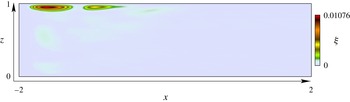
is used to locate regions likely to be absolutely unstable. The wavemaker
 $\unicode[STIX]{x1D709}(x,0,z)$
is shown in figure 16 where region near the unstable boundary seems to play an important role. These contours have their greatest magnitude bellow the boundary
 $b=0$
, near to the top-left corner, where the descending plume originates. These results are in agreements with the local stability analysis of Tsai et al. (Reference Tsai, Hussam, Fouras and Sheard2016) where this region was found to be the most convectively unstable.
Structural sensitivity vector
 $\unicode[STIX]{x1D709}(x,0,z)$
associated with the most unstable two-dimensional mode (
 $\unicode[STIX]{x1D6FD}=0$
), at
 $Ra=6.4\times 10^{7}$
and
 $Pr=1$
for no-slip boundary conditions.

In the following, we define the streamfunction for the perturbation such that
 $$\begin{eqnarray}\frac{\unicode[STIX]{x2202}\unicode[STIX]{x1D719}}{\unicode[STIX]{x2202}z}=u^{\prime },\quad \frac{\unicode[STIX]{x2202}\unicode[STIX]{x1D719}}{\unicode[STIX]{x2202}x}=-w^{\prime }.\end{eqnarray}$$
Different velocity profiles
 $U(z)$
and buoyancy profiles
 $B(z)$
for the streamwise positions between
 $x_{p}=-1.375$
and
 $x_{p}=-1.525$
have been considered where the wavemaker dominates. A local linear stability analysis is performed for parallel flow profiles
 $(U(x_{p},z),0,B(x_{p},z))$
using normal modes of the form
 $$\begin{eqnarray}(\unicode[STIX]{x1D719},b^{\prime })=(\hat{\unicode[STIX]{x1D719}}(z),\hat{b}(z))\,\text{e}^{-\text{i}(\unicode[STIX]{x1D714}t-\unicode[STIX]{x1D6FC}x)}.\end{eqnarray}$$
Linearizing the Navier–Stokes system at
 $(U(z),0,B(z))$
and taking the curl of (2.1) in the
 $(x{-}z)$
plane, the Orr–Sommerfeld equation is coupled to the buoyancy such that
 $$\begin{eqnarray}\displaystyle \left[(-\text{i}\unicode[STIX]{x1D714}+\text{i}\unicode[STIX]{x1D6FC}U(x_{p},z))\unicode[STIX]{x1D6FB}^{2}-\text{i}\unicode[STIX]{x1D6FC}U^{\prime \prime }(x_{p},z)-\left(\frac{A^{3}Pr}{Ra}\right)^{1/2}\unicode[STIX]{x1D6FB}^{4}\right]\hat{\unicode[STIX]{x1D719}} & = & \displaystyle \text{i}\unicode[STIX]{x1D6FC}\hat{b},\quad\end{eqnarray}$$
 $$\begin{eqnarray}\displaystyle \left[-\text{i}\unicode[STIX]{x1D714}+\text{i}\unicode[STIX]{x1D6FC}U(x_{p},z)-\left(\frac{A^{3}}{PrRa}\right)^{1/2}\unicode[STIX]{x1D6FB}^{2}\right]\hat{b} & = & \displaystyle \text{i}\unicode[STIX]{x1D6FC}\frac{\unicode[STIX]{x2202}B(x_{p},z)}{\unicode[STIX]{x2202}z}\hat{\unicode[STIX]{x1D719}}.\qquad\end{eqnarray}$$
 $D(\unicode[STIX]{x1D714},\unicode[STIX]{x1D6FC})=0$
. A spatio-temporal linear stability analysis has been performed, solving
 $\unicode[STIX]{x1D714}(\unicode[STIX]{x1D6FC})$
for both complex wavenumbers
 $\unicode[STIX]{x1D6FC}$
and frequencies
 $\unicode[STIX]{x1D714}$
. Solving
 $\unicode[STIX]{x1D714}(\unicode[STIX]{x1D6FC})$
, the complex local absolute frequency is given in classical fashion by
 $$\begin{eqnarray}\unicode[STIX]{x1D714}_{0}=\unicode[STIX]{x1D714}(\unicode[STIX]{x1D6FC}_{0}),\quad \text{with }\frac{\unicode[STIX]{x2202}\unicode[STIX]{x1D714}}{\unicode[STIX]{x2202}\unicode[STIX]{x1D6FC}}(\unicode[STIX]{x1D6FC}_{0})=0.\end{eqnarray}$$
The locally parallel flow defined by the local profile
 $(U(x_{p},z),0,B(x_{p},z))$
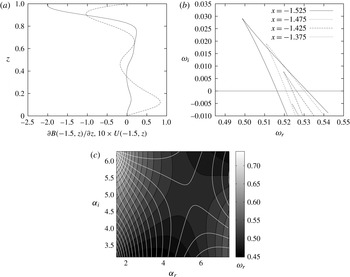
is absolutely unstable if the imaginary part of the complex absolute frequency is positive (Schmid & Henningson Reference Schmid and Henningson2001; Chomaz Reference Chomaz2005). Note that in the present vertical profiles, the fluid near the top boundary is unstable (cf. figure 17
a). This was confirmed by the local stability analysis where the unstable eigenfunctions were only found near the upper boundary. Figure 17(b) depicts the analysis for the local profiles from
 $x=-1.375$
(dotted line) until
 $x=-1.525$
(continuous line). The
 $\unicode[STIX]{x1D6FC}_{i}=\text{Const.}$
contours (for
 $0.45<\unicode[STIX]{x1D6FC}_{r}<0.7$
) in the complex frequency plane are shown and the cusp (the point
 $(\unicode[STIX]{x2202}\unicode[STIX]{x1D714})/(\unicode[STIX]{x2202}\unicode[STIX]{x1D6FC})(\unicode[STIX]{x1D6FC}_{0})=0$
) appears for
 $\unicode[STIX]{x1D6FC}_{r}\approx 5.98$
,
 $\unicode[STIX]{x1D6FC}_{i}\approx 5.25$
, under and above the real axis for
 $x=-1.375$
and
 $x=-1.425$
respectively. The saddle point described in (6.9) is shown in figure 17(c) where the pinching point between two distinct branches
 $\unicode[STIX]{x1D6FC}+$
and
 $\unicode[STIX]{x1D6FC}-$
(
 $\unicode[STIX]{x1D6FC}$
complex and
 $\unicode[STIX]{x1D714}_{i}$
constant) originate from distinct halves of the
 $\unicode[STIX]{x1D6FC}-$
plane (Schmid & Henningson Reference Schmid and Henningson2001). These results demonstrate that the flow becomes absolutely unstable near the upper boundary, in the vicinity of the plume. Prior to the discussion in § 4, we investigated the effect of both shear and viscosity on the local stability properties of the flow. In the present local stability analysis at
 $x_{p}=-1.525$
, decreasing viscosity only has a weak effect on the local stability, but increasing the magnitude of the shear stabilizes the flow.
Longitudinal velocity
 $U(x_{p},z)$
(- - -) and Brunt–Väisälä frequency profiles
 $\unicode[STIX]{x2202}B(x_{p},z)/\unicode[STIX]{x2202}z$
(——) (a) located near the plume at
 $x_{p}=-1.525$
, using no-slip boundary conditions. Contours in the plane (
 $\unicode[STIX]{x1D714}_{r},\unicode[STIX]{x1D714}_{i}$
) at
 $x_{p}=-1.525$
(——) and
 $x_{p}=-1.475$
(- - -) at
 $x_{p}=-1.425$
(- - -) and
 $x_{p}=-1.375$
(
 $\ldots$
) at
 $\unicode[STIX]{x1D6FC}_{i}=5.25$
, (cusp map
 $(\unicode[STIX]{x2202}\unicode[STIX]{x1D714}(\unicode[STIX]{x1D6FC}_{0}))/(\unicode[STIX]{x2202}\unicode[STIX]{x1D6FC})=0$
) (b). Spatial branches in the complex
 $\unicode[STIX]{x1D6FC}$
-plane for
 $Ra=6.4\times 10^{7}$
showing the saddle point for iso-contours of
 $\unicode[STIX]{x1D714}_{r}$
(c) and where the white lines show the saddle point associated with the growth rate
 $\unicode[STIX]{x1D714}_{i}$
.

Comparing these local results with the global stability analysis, both the growth rate and the longitudinal wavenumber of the instability compare favourably (
 $\unicode[STIX]{x1D714}_{0,i}=0.0291$
versus
 $\unicode[STIX]{x1D714}_{global,i}=0.0307$
(cf. figure 12
a) and
 $\unicode[STIX]{x1D6FC}_{0}\approx 5.42$
versus
 $\unicode[STIX]{x1D6FC}_{global}\approx 5.2$
). Despite this good agreement in the wavenumber and growth rate, the global frequency
 $\unicode[STIX]{x1D714}_{0,r}=0.498$
is smaller than the global frequency
 $\unicode[STIX]{x1D714}_{global,r}=0.574$
The spatial growth rate
 $\unicode[STIX]{x1D6FC}_{i}\approx 5.25$
is large, meaning that the mode decays very fast towards the centre of the domain, in agreement with the modal structure of the global instability, but the global mode is influenced by the non-parallel nature of the flow as
 $x\rightarrow -2$
. Thus it seems unlikely that non-parallel effects can be neglected. A fundamental assumption of the local stability analysis is the existence of two separate length scales in the flow: the evolution length scale
 $\unicode[STIX]{x1D706}$
, characterizing the spatial development of the base flow, and the instability wavelength,
 $2\unicode[STIX]{x03C0}/(\unicode[STIX]{x1D6FC}_{0})\approx 1$
. The length scale
 $\unicode[STIX]{x1D706}$
can be defined by means of the momentum or vorticity thickness of the base flow profiles
 $\unicode[STIX]{x1D6E9}=\unicode[STIX]{x1D6E9}(x)$
and writes
 $$\begin{eqnarray}\unicode[STIX]{x1D706}\sim \left(\frac{1}{\unicode[STIX]{x1D6E9}}\frac{\text{d}\unicode[STIX]{x1D6E9}}{\text{d}x}\right)^{-1}.\end{eqnarray}$$
The small parameter of interest is then
 $$\begin{eqnarray}\unicode[STIX]{x1D716}\sim \frac{\unicode[STIX]{x1D6FC}_{0}}{\unicode[STIX]{x1D706}}\ll 1.\end{eqnarray}$$
In the present investigations, both the velocity
 $U(z)$
and the buoyancy profiles
 $B(z)$
of the base flow evolve rapidly near the upper boundary. In this region, the parameter
 $\unicode[STIX]{x1D716}\approx 2$
shows that a weakly non-parallel asymptotic analysis is impossible. The same issue was reported for instance in the case of a separated flow behind a bump where the absolute frequency
 $\unicode[STIX]{x1D714}_{0,r}$
(Marquillie & Ehrenstein Reference Marquillie and Ehrenstein2003) did not match the global instability
 $\unicode[STIX]{x1D714}_{global,r}$
(Ehrenstein & Gallaire Reference Ehrenstein and Gallaire2008) due to the rapid evolution of the base flow near the reattachment region. We conclude that the two-dimensional instability is associated with a local absolutely unstable sheared Rayleigh–Taylor instability controlled by non-parallel effects near the plume region.
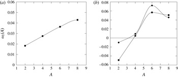
Growth rate
 $\unicode[STIX]{x1D714}_{i}$
extracted from the global stability as a function of the domain’s aspect ratio
 $A=L/H$
, for the most unstable three-dimensional mode (-▪-) and the two-dimensional mode (-●-) at
 $Ra=A^{3}2.26\times 10^{6}$
for free-slip boundary conditions (a) and
 $Ra=A^{3}3\times 10^{6}$
for no-slip boundary conditions (b) at
 $Pr=1$
.

7 Effect of the aspect ratio on the stability
The previous stability analyses show that a competition exists between the three-dimensional longitudinal rolls and the two-dimensional instability shed by the plume. Questions remain concerning the effect of the aspect ratio
 $A$
, the Prandtl number
 $Pr$
and the boundary conditions on the stability and whether one mode dominates the dynamics. Here we consider variations in
 $A$
and the aforementioned global stability calculations have been repeated using the global stability varying the computational domain length’s
 $L$
.
For both free-slip and no-slip boundary conditions, the evolution of the largest growth rate
 $\unicode[STIX]{x1D714}_{i}$
as a function of the aspect ratio
 $A$
is shown in figure 18(a,b) respectively in the range
 $A=[2,8]$
. For the present parameter range, the three-dimensional instability appears to increase almost linearly in the case of free-slip boundary conditions. In the case of no-slip boundary conditions, and an aspect ratios
 $A>3.85$
, both instabilities are active, whereas for
 $A<3.2$
, the flow is globally stable.
For the large values of
 $A$
, the growth rates seem to saturate at
 $0.05$
for the most unstable longitudinal rolls and attain a maximum for
 $\unicode[STIX]{x1D714}_{i}\approx 7.2\times 10^{-2}$
for the two-dimensional mode. The value for the most unstable wavelength
 $\unicode[STIX]{x1D6FD}\approx 6$
remains essentially constant throughout the entire parameter range, suggesting that for large values of
 $A$
, the instabilities are mostly controlled by the diffusion of the stratifying agent and the viscosity.
8 Conclusions
The global stability of a rectangular cavity in horizontal convection was investigated using direct numerical simulations of the two-dimensional base flow at a Prandtl number equal to unity. The boundary conditions are idealized using free-slip and no-slip boundaries for the velocity and an imposed buoyancy profile, which are comparable with previous results (Gayen et al. Reference Gayen, Griffiths and Hughes2014).
Three-dimensional stability modes computed for two-dimensional base flows using free-slip boundary conditions show that the flow becomes globally unstable at a critical Rayleigh number
 $Ra_{c,3D}\approx 2.02\times 10^{7}$
where three-dimensional steady longitudinal rolls appear for a transverse wavenumber
 $\unicode[STIX]{x1D6FD}\approx 6$
. The mechanism at the origin of this instability is shown to be of Rayleigh–Taylor type. A WKB analysis along streamlines shows that it is possible to build an inviscid global mode using as local necessary condition for instability,
 $Ri<0$
. Following the same procedure for the elliptical or the centrifugal instability analysis in vortices, the global mode can be reconstructed by means of viscous and asymptotic boundary layer theory, where the transverse wave length and the growth rate appear to scale as
 $Ra^{-1/6}$
while freezing the base state.
In the case of no-slip boundary conditions, instabilities set in at a higher Rayleigh number and the flow is shown to become unstable with respect to both three- and two-dimensional perturbations, with a critical Rayleigh number at
 $Ra_{c,2D}\approx 1.65\times 10^{8}$
. These results are in qualitative agreement with the local temporal stability analyses of Tsai et al. (Reference Tsai, Hussam, Fouras and Sheard2016) where a similar scenario is described.
The two-dimensional mode belongs to a different family than the three-dimensional instability and is associated with the vortex shedding of the plume, entraining alternatively heavier and lighter fluid parcels towards the bottom. This mode is shown to have a similar amplification rate to the longitudinal rolls but appears to play an important role in the dynamics, as reported by Gayen et al. (Reference Gayen, Griffiths and Hughes2014) in their direct numerical simulations. The local spatio-temporal stability of parallel profiles near the plume shows that the flow becomes absolutely unstable. This instability is also related to the Rayleigh–Taylor instability, has a larger growth rate than the pure longitudinal rolls for all values of
 $Ra$
investigated, and are unstable for small transverse wavenumbers in the range
 $\unicode[STIX]{x1D6FD}=[0:3]$
.
At the onset of instability for the no-slip case (i.e.
 $Ra=1.92\times 10^{8}$
), the effect of the aspect ratio of the domain on the global stability is also studied. The two and three-dimensional instabilities are shown to be either stable for
 $A<3.2$
either unstable for
 $A>3.85$
.
The growth rates of both instabilities appear to behave similarly with respect to variations in
 $A$
. However at
 $A=8$
, both growth rates attain a maximum with the three-dimensional instability having a slightly larger growth rate. The maximum growth rate for the two-dimensional instability reaches a maximum at
 $A=6$
with
 $\unicode[STIX]{x1D714}_{i}=7.2\times 10^{-2}$
. The stability for the free-slip case is analysed at
 $A^{-3}Ra=2.26\times 10^{6}$
where the growth rate of the longitudinal rolls evolves essentially linearly with
 $A$
in the range
 $A=[2:8]$
.
Iso-contours of the growth rate
 $\unicode[STIX]{x1D714}_{i}$
associated with the most unstable mode as a function of the transverse wavenumber
 $\unicode[STIX]{x1D6FD}$
and
 $A^{-3}Ra$
for the free-slip case (a) and the no-slip case (b). The dashed line represents the marginal stability curve (
 $\unicode[STIX]{x1D714}_{i}=0$
).

The no-slip results are also in relatively good agreements with the stability transition found in the direct numerical simulation of Gayen et al. (Reference Gayen, Griffiths and Hughes2014). The onset of instability was found in the range
 $Ra=[5.87\times 10^{7}\,5.87\times 10^{8}]$
for
 $A=6.25$
and in the range of the value of
 $Ra_{c,2D}\approx 1.65\times 10^{8}$
reported in the present study. These results also agree with the prediction from the effect of
 $A$
on the stability. Also, the width of the domain considered in Gayen et al. (Reference Gayen, Griffiths and Hughes2014), using our units was
 $W=0.25$
. However, our stability analysis predicts that the most unstable three-dimensional modes have an unstable wavenumber
 $\unicode[STIX]{x1D6FD}\approx 12$
which translates in a wavelength close
 $2\unicode[STIX]{x03C0}/\unicode[STIX]{x1D6FD}\approx 0.5$
which is twice longer than the width of their domain. This would explain why the three-dimensional instability appears later in their DNS than in our stability analysis.
The present results are summarized in figure 19(a,b) where the most unstable growth rates are mapped in the
 $(Ra,\unicode[STIX]{x1D6FD})$
plane for both types of boundary conditions. The marginal stability is reported using a dashed line and shows the onset of two and three-dimensional instabilities. As mentioned earlier, there is a change of behaviour, characterized by kink of
 $\unicode[STIX]{x1D714}_{i}$
in the
 $(Ra,\unicode[STIX]{x1D6FD})$
plane visible a
 $Ra\approx 6.4\times 10^{8}$
in the free-slip case. In the no-slip case, a similar behaviour was found for
 $Ra\approx 6.4\times 10^{9}$
but was not reported in the present manuscript. This change was reported earlier in the stability analysis for the free-slip case, and seems to correspond to the stability transition reported in direct numerical simulation of Gayen et al. (Reference Gayen, Griffiths and Hughes2014), in the range
 $[2.68\times 10^{8}\,2.68\times 10^{9}]$
, where the flow was found to transition to turbulence.
In a forthcoming manuscript, this behaviour will be shown to be related to the bifurcation of the base flow, leading to the plume reflection mechanism and the transition to turbulence.
Acknowledgements
The authors acknowledge the support by the National Science Foundation under grant OCE-1155558. The authors also wish to acknowledge the anonymous referees for their thorough reviews and suggestions.