

1. Introduction
1·1. Background
Surfaces of mean curvature zero in the Heisenberg group
 $\mathcal{H}$
, equipped with a left-invariant Riemannian metric, denoted here
 $\text{Nil}^{3}$
, have been studied by many authors. Berdinskii and Taimanov [Reference Berdinskii and Taimanov1] gave a spinor type representation, similar to other so-called integrable classes of surfaces such as constant mean curvature surfaces in space forms. One can show ([Reference Daniel7, Reference Figueroa10, Reference Figueroa11]) that they are related to harmonic maps into the hyperbolic space
 $\mathbb{H}^2$
as follows: the Gauss map of an immersion f into
 $\text{Nil}^{3}$
is the left translation
 $N=f^{-1}n$
of the unit normal. The surface is called vertical at a point p if
 $N_p$
is parallel to the
 $e_1e_2$
-plane. The Gauss map of a nowhere vertical minimal surface in
 $\text{Nil}^{3}$
is harmonic into the hemisphere equipped with the hyperbolic metric, and conversely a nowhere holomorphic harmonic map into
 $\mathbb{ H}^2$
is the Gauss map of a minimal surface. This allows one to use the theory of harmonic maps to study these surfaces (see, e.g., [Reference Cartier5, Reference Dorfmeister, Inoguchi and Kobayashi8]).
If one considers now Lorentzian metrics on
 $\mathcal{H}$
, Rahmani [Reference Rahmani22] showed that there are (up to homothety) three different choices of left-invariant metric (see section 2 below),
 $g_1$
,
 $g_2$
and
 $g_3$
, according to whether the 1-dimensional center of the Lie algebra is spacelike, timelike or null in the metric. A classical Weierstrass-type representation exists for mean curvature zero surfaces in such spaces ([Reference Cintra, Mercuri and Onnis6, Reference Lira, Melo and Mercuri19]), but the Weierstrass data need to satisfy non-trivial extra conditions; hence only simple examples of mean curvature zero surfaces in these manifolds have been given. For spacelike surfaces in the case of the metric
 $g_2$
(see [Reference Lee18] and this paper), and for timelike surfaces with the metric
 $g_1$
(see [Reference Kiyohara and Kobayashi16]), a relationship between harmonic maps and mean curvature zero surfaces, similar to the Riemannian case exists. This allows one to use loop group methods to construct all solutions, and, in particular, generate many more examples.
Here we will study spacelike mean curvature zero surfaces in
 $\mathcal{H}$
equipped with the metric
 $g_2$
, denoting this space by
 ${\text{Nil}^{3}_{1}}$
, via the relationship with harmonic maps into
 $\mathbb{S}^2$
.
1·2. Surfaces with harmonic Gauss maps
Harmonic maps from a Riemann surface into
 $\mathbb{S}^2$
are directly related to various different geometric problems, via the Gauss map. In these cases, the passage from the harmonic Gauss map to the surface is well defined even at points where the resulting surface is not regular (a so-called frontal), so it is natural in this context to consider generalised surfaces with singularities.
Given a harmonic map
 $\nu\,:\, M \to \mathbb{S}^2$
, where M is a simply connected Riemann surface, there are naturally associated:
-
(1) a geometrically unique constant positive Gaussian curvature
 $K=1$
, surface
$f_{cgc} : \to \mathbb{R}^3$
(see, e.g. [Reference Brander3]), satisfying a compatible pair of linear PDE: that has
\begin{equation*} f_z = i \nu \times \nu_z, \end{equation*}
$\nu$
as its Gauss map. Here
$z=x+iy$
and
$f_z:= (1/2)(\partial f/\partial x-i\partial f/\partial y)$
;
-
(2) a pair of geometrically unique constant mean curvature (CMC)
$H=1/2$
surfaces
$f^{\pm}\,:\, M \to \mathbb{R}^3$
that are parallel surfaces to
$f_{cgc}$
, given by:
\begin{equation*} f^\pm = f_{cgc} \pm \nu; \end{equation*}
-
(3) a 2-dimensional family of zero mean curvature spacelike surfaces f in
${\text{Nil}^{3}_{1}}$
, to be described below.





Conversely, such surfaces have harmonic Gauss maps.
The way that singularities appear in each case is different however: evidently
 $f_{cgc}$
is regular if and only if the harmonic map N is also regular, by the relation
 $f_z = i N \times N_z$
.
For the second case, the CMC surface
 $f^\pm$
has derivatives:
 \begin{equation} f^\pm_x = \nu \times \nu_y \, \pm \nu_x, \quad \quad f^\pm_y = -\nu \times \nu_x \, \pm \nu_y.\end{equation}
It follows that
 $f^\pm$
only has singularities of rank zero (branch points), and these occur precisely when
 \begin{equation*} \nu_x = \mp \nu \times \nu_y.\end{equation*}
If
 $\nu$
itself has rank zero at a point (i.e.
 $\nu_x=\nu_y=0$
), then both
 $f^+$
and
 $f^-$
have a branch point. If
 $\nu_x = \mp \nu \times \nu_y \neq 0$
, then
 $f^\pm$
has a branch point, and, one can show,
 $f^\mp$
has an umbilic point.
For the third case, the fact that the metric on
 ${\text{Nil}^{3}_{1}}$
is not isotropic means that a given harmonic map
 $\nu$
into
 $\mathbb{S}^2$
can be interpreted in many geometrically distinct ways as the Gauss map for a surface in
 ${\text{Nil}^{3}_{1}}$
. The Lie algebra
 ${\mathfrak{nil}_{1}^{3}}$
is identified with the vector space
 $\mathbb{R}^3$
, with the center of
 ${\mathfrak{nil}_{1}^{3}}$
spanned by
 $e_3$
. If we fix the given embedding of
 $\mathbb{S}^2$
in
 $\mathbb{R}^3$
, with the north pole pointing in the
 $e_3$
direction, then we obtain a well defined mean curvature zero surface
 $f: M \to {\text{Nil}^{3}_{1}}$
(described below). If we apply an isometry to
 $\mathbb{S}^2$
, then this has no geometric significance to
 $\nu$
. However, a rotation about any axis other than the
 $e_3$
-axis is not an isometry of
 ${\text{Nil}^{3}_{1}}$
, and so there is a 2-dimensional family of surfaces
 $f: M \to {\text{Nil}^{3}_{1}}$
associated to the harmonic map
 $\nu$
. As for the singularities, f will have singularities exactly at points where
 $\nu$
is perpendicular to
 $e_3$
, i.e. when
 $\nu$
takes values in the equator in the
 $e_1 e_2$
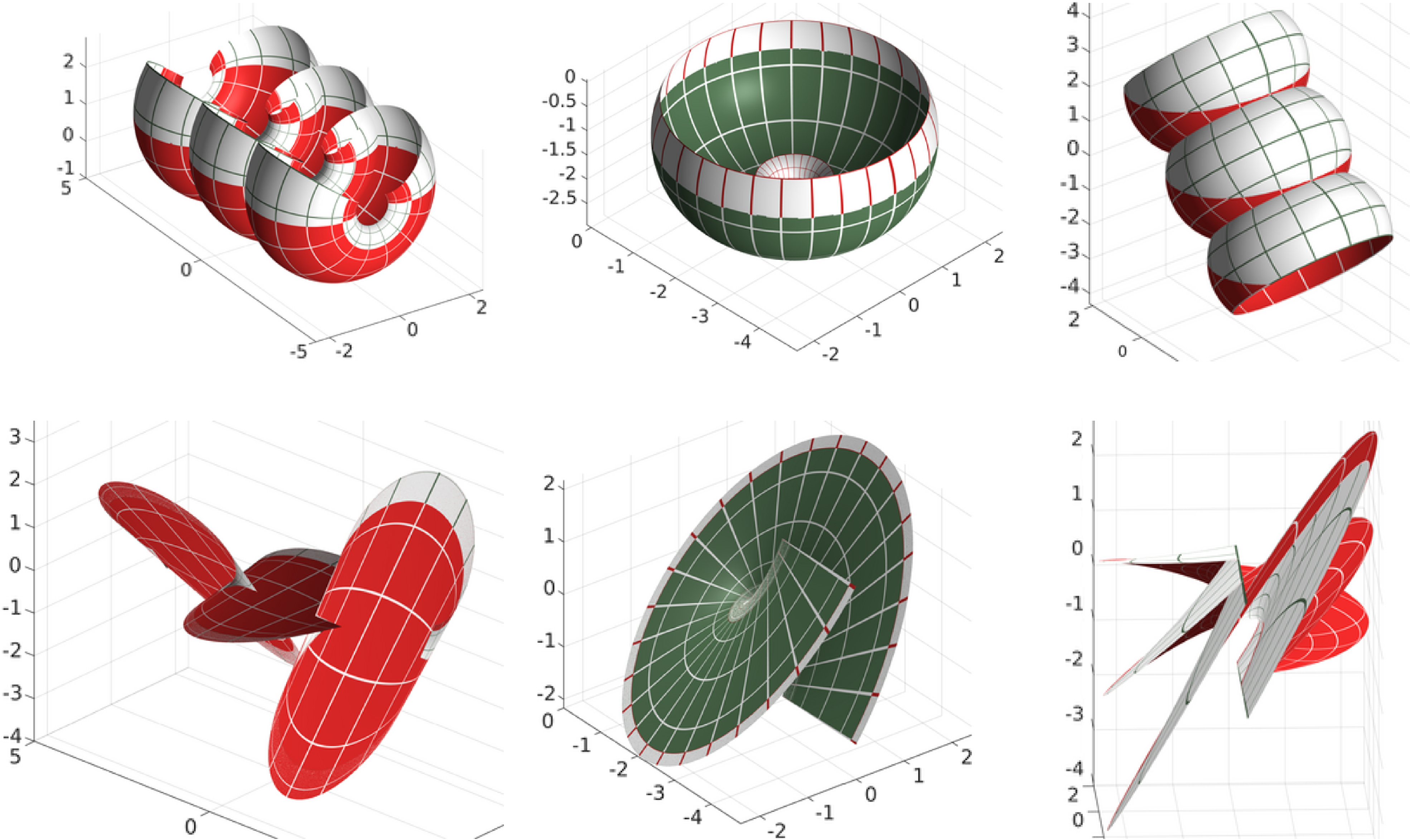
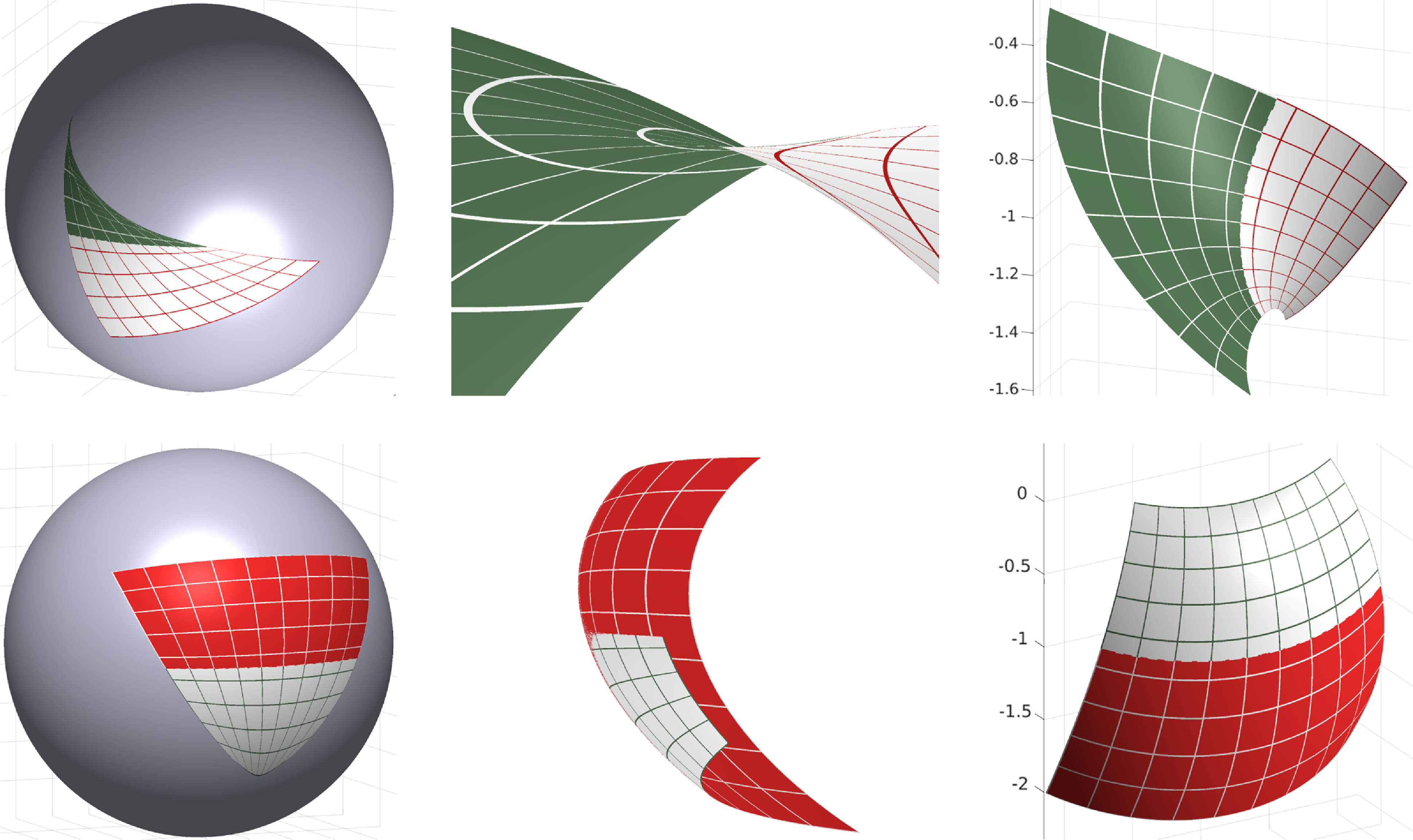
-plane. Hence the singular set is different for each surface in the 2-parameter family (see Figure 1, and Examples 3·9 and 3·10).
Top: Portions of a single constant mean curvature surface of revolution, with three different spatial orientations. Bottom: the corresponding maximal surfaces in
 ${\text{Nil}^{3}_{1}}$
, in the same order. (Example 3·9.)

1·3. Surfaces with singularities
It is well known that there are no complete maximal surface in the Lorentzian 3-space
 $\mathbb{L}^3$
besides the plane. Nevertheless, such surfaces are naturally of interest to geometers, and this motivated the definition of a maxface [Reference Umehara and Yamada23] as a generalised surface with singularities. For maxfaces, the Gauss map is a holomorphic map into the extended hyperbolic plane, and the surface has singularities where the Gauss map takes values in the boundary between the two components. The generic singularities are cuspidal edge, swallowtail and cuspidal cross-cap [Reference Fujimori, Saji, Umehara and Yamada12].
In contrast to this, for maximal surfaces in
 ${\text{Nil}^{3}_{1}}$
, the Gauss map is a nowhere holomorphic harmonic map into
 $\mathbb{S}^2$
. However, we will show that the generic singularities are of the same type as for maxfaces.
1·4. Outline of this paper
In section 2 we briefly describe the Heisenberg group and the left-invariant Lorentzian metric we will use. In section 3 we describe the spinor representation for maximal surfaces in
 ${\text{Nil}^{3}_{1}}$
, the relation with harmonic maps into
 $\mathbb{S}^2$
, and how to produce all solutions via loop group methods.
In section 4 we prove that the generic singularities are cuspidal edge, swallowtail and cuspidal cross-cap: theorem 4·1 and theorem 4·4 characterise these singularities respectively in terms of the conformal Gauss map and the Abresch–Rosenberg differential. This gives (in theorem 4·9) a characterisation of the generic singularities in the space of local solutions.
In section 5 we show how to solve the Cauchy problem for a harmonic map into
 $\mathbb{S}^2$
(theorem 5·1) via loop group methods, which is of independent interest. This allows one to construct harmonic maps with prescribed transverse derivative along any curve in the sphere: in particular, the equator, and thus with a prescribed singular set along a curve (theorem 5·3). theorem 5·4 shows explicitly the relation between the geometry of the Cauchy data and the type of generic singularity at a point.
In section 6 we look at the geometry of the curve on the associated CMC surface that corresponds to the equator in
 $\mathbb{S}^2$
for the harmonic Gauss map. This curve gives a very simple characterisation of the generic singularities of the maximal surface in
 ${\text{Nil}^{3}_{1}}$
. As an application, we show in theorem 6·4 that a regular spacelike maximal disc with null boundary in
 ${\text{Nil}^{3}_{1}}$
must have at least two cuspidal cross-caps on the boundary.
Numerics. The DPW method for harmonic maps can be implemented numerically to compute solutions from a given potential. At the time of writing, implementations in Matlab that allow one to compute the examples shown here, as well as any other solution with given Cauchy data, can be found at http://davidbrander.org/software.html
2. Left invariant metrics on the Heisenberg group
The 3-dimensional Heisenberg group
 $\mathcal{H}$
is the group of
 $3\times 3$
real upper-triangular matrices with one’s on the diagonal. The Lie algebra
 $\mathfrak{h}$
is spanned by:
 \begin{equation*} a_1 = \begin{pmatrix} 0 &\quad 1 &\quad 0\\0&\quad 0&\quad 0\\0&\quad 0&\quad 0\end{pmatrix}, \quad a_2 = \begin{pmatrix} 0 &\quad 0 &\quad 0\\0 &\quad 0 &\quad 1\\0&\quad 0&\quad 0\end{pmatrix}, \quad a_3 = \begin{pmatrix} 0 &\quad 0 &\quad 1\\0&\quad 0&\quad 0\\0&\quad 0&\quad 0\end{pmatrix},\end{equation*}
with commutators,
 $[a_1,a_2]=a_3$
and
 $[a_1,a_3]=[a_2,a_3]=0$
. For this group, exponential coordinates give a bijection
 $\exp:\, \mathfrak{h} \to \mathcal{H}$
, with the formula:
 \begin{equation} \exp(x_1 a_1 + x_2 a_2 +x_3a_3) = \begin{pmatrix} 1&\quad x_1&\quad x_3+\frac{1}{2}x_1x_2\\ 0 &\quad 1 &\quad x_2\\ 0 &\quad 0 &\quad 1 \end{pmatrix}.\end{equation}
Thus, identifying
 $\mathcal{H}$
with
 $\mathfrak{h} = \mathbb{R}^3$
, it is common to represent
 $\mathcal{H}$
as
 $\mathbb{R}^3$
with the group structure that corresponds to the matrix product in
 $\mathcal{H}$
, namely:
 \begin{equation*} (x_1,x_2,x_3)\cdot(\tilde x_1,\tilde x_2, \tilde x_3) = (x_1+\tilde x_1, \,\, x_2+\tilde x_2, \,\, x_3+\tilde x_3 + \tfrac{1}{2}(x_1\tilde x_2 - \tilde x_1 x_2)).\end{equation*}
Differentiating the map
 $L_X: \mathbb{R}^3 \to \mathbb{R}^3$
, given by
 $L_X(\tilde X)=X\cdot \tilde X$
, at
 $\tilde X= e = (0,0,0)$
, we have:
 \begin{equation*} \textrm{d} L_X |_e = \begin{pmatrix} 1 &\quad 0 &\quad 0 \\ 0 &\quad 1 &\quad 0 \\ -\tfrac{1}{2}x_2 &\quad \tfrac{1}{2} x_1 &\quad 1 \end{pmatrix},\end{equation*}
so the left invariant vector fields generated by
 $a_1$
,
 $a_2$
and
 $a_3$
are:
 \begin{equation} A_1 = \frac{\partial}{\partial x_1} - \frac{x_2}{2}\frac{\partial }{\partial x_3} ,\quad \quad A_2 = \frac{\partial}{\partial x_2} + \frac{x_1}{2}\frac{\partial }{\partial x_3} ,\quad \quad A_3 = \frac{\partial }{\partial x_3}.\end{equation}
2·1. Left invariant Riemannian metrics
Milnor [Reference Milnor20] introduced a systematic study of left invariant Riemannian metrics on Lie groups. On a connected Lie group of dimension 3, the Lie bracket is necessarily given by
 $[u,v]=L(u \times v)$
, where L is linear and the cross-product is defined with respect to a chosen orientation. The group is unimodular if and only if the linear map L is self-adjoint. Using this, Milnor showed that, for the case of a 3-dimensional unimodular Lie group G, a basis
 $\{e_1, e_2, e_3\}$
can be chosen for the Lie algebra that is orthonormal with respect to the given metric and for which the Lie bracket is given by
 \begin{equation*}[e_1, e_2]=\lambda_3 e_3, \quad[e_2,e_3]=\lambda_1 e_1, \quad[e_3, e_1]=\lambda_2 e_2.\end{equation*}
For the case of the Heisenberg group
 $\mathcal{H}$
, with notation as above, since all commutators are proportional to
 $a_3$
, it follows that one of the
 $e_j$
, which we may as well take to be
 $e_3$
, is proportional to
 $a_3$
. Then
 $\lambda_1=\lambda_2=0$
,
 $\lambda_3 \neq 0$
, and no generality is lost by assuming that
 \begin{equation*}e_1=a_1, \quad e_2 = a_2, \quad e_3 = \frac{1}{\lambda_3} a_3.\end{equation*}
Since the orientation can be chosen so that
 $\lambda_3\gt0$
, there is, up to a positive homothety, only one left invariant metric on
 $\mathcal{H}$
.
2·2. Left invariant Lorentzian metrics
Rahmani [Reference Rahmani22] studied the Lorentzian metric version of this problem for 3-dimensional unimodular Lie groups, using a similar approach to Milnor’s. Since a Lorentzian metric is not isotropic, there are more possibilities. One can again choose an orthonormal basis for the Lie algebra, with
 \begin{equation*}\langle e_1, e_1 \rangle = \langle e_2, e_2 \rangle =1,\quad \langle e_3, e_3 \rangle =-1,\end{equation*}
and the Lie bracket is given by
 $[u, v]=L (u \times v)$
, where L is linear and the Lorentzian cross-product is defined by
 $e_1 \times e_2 = - e_3$
,
 $e_2 \times e_3 = e_1$
,
 $e_3 \times e_1 = e_2$
. Here, also, the group is unimodular if and only if L is self-adjoint. The different possible Lie algebra structures in terms of the orthonormal basis are given in [Reference Rahmani22]; among these, there are three that give the Heisenberg group structure:
-
1.
$[e_1,e_2]=[e_1,e_3]=0$
,
$[e_2,e_3]=\mu e_1$
. -
2.
$[e_2,e_3]=[e_1,e_3]=0$
,
$[e_1,e_2]= \mu e_3$
. -
3.
$[e_2,e_3]=0$
,
$[e_3, e_1]=[e_2,e_1]=e_2-e_3$
.



These correspond to the center
 $\text{Span} \{a_3\}$
of
 $\mathfrak{h}$
being spacelike, timelike, or null: for the three cases we respectively have
 $a_3= \mu e_1$
,
 $a_3= \mu e_3$
and
 $a_3=e_3-e_2$
. The corresponding left invariant Lorentzian metrics are denoted respectively by
 $g_1$
,
 $g_2$
and
 $g_3$
. The algebra of Killing fields is given for each case in [Reference Rahmani22], showing that the isometry groups are of dimension 4 for
 $g_1$
and
 $g_2$
, and of dimension 6 for the case of
 $g_3$
. The geometry of the metrics
 $g_1$
,
 $g_2$
and
 $g_3$
is studied further by N. Rahmani and S. Rahmani in [Reference Rahmani and Rahmani21]. They prove that the metrics are nonisometric, and that
 $g_3$
is flat.
3. Maximal spacelike surfaces in
${{\rm Nil}^{3}_{1}}$

In this paper, we use the metric
 $g_2$
, in particular with
 $\mu=1$
, taking
 \begin{equation*}e_1=a_1, \quad e_2=a_2, \quad e_3=a_3,\end{equation*}
as the orthonormal basis for the Lorentzian metric. In the coordinates
 $(x_1,x_2,x_3)$
for
 $\mathbb{ R}^3=\mathfrak{h}\equiv\mathcal{H}$
, we have from (2·2):
 \begin{equation*} \frac{\partial }{\partial x_1} = e_1 + \frac{x_2}{2}e_3, \quad \quad \frac{\partial }{\partial x_2} = e_2 - \frac{x_1}{2}e_3, \quad \quad \frac{\partial }{\partial x_3}=e_3,\end{equation*}
in terms of the left invariant vector fields
 $e_i= a_i$
. Using the Lorentzian orthonormality, with
 $\langle e_3,e_3\rangle = -1$
, this gives the metric in the coordinate frame:
 \begin{equation*}g_2 = \textrm{d} x_1^2+\textrm{d} x_2^2 -\left(\textrm{d} x_3 + \frac{1}{2}(x_2 \textrm{d} x_1 - x_1 \textrm{d} x_2)\right)^2.\end{equation*}
The Levi-Civita connection
 $\nabla$
of
 $g_2$
is given by
 \begin{equation*} \begin{pmatrix} \nabla_{e_1} e_1 &\quad \nabla_{e_1} e_2 &\quad \nabla_{e_1} e_3 \\[4pt] \nabla_{e_2} e_1 &\quad \nabla_{e_2} e_2 &\quad \nabla_{e_2} e_3 \\[4pt] \nabla_{e_3} e_1 &\quad \nabla_{e_3} e_2 &\quad \nabla_{e_3} e_3 \end{pmatrix} = \begin{pmatrix} 0 &\quad \tfrac{1}{2} e_3&\quad \tfrac{1}{2} e_2\\[4pt] -\tfrac{1}{2} e_3 &\quad 0 &\quad - \tfrac{1}{2} e_1\\[4pt] \tfrac{1}{2} e_2 &\quad -\tfrac{1}{2} e_1&\quad 0 \end{pmatrix}.\end{equation*}
Then it is easy to see the symmetric bi-linear map given by
 $\{e_i, e_j\} = \nabla_{e_i} e_j + \nabla_{e_j} e_i$
satisfies
 \begin{equation*} \{e_1, e_2\}=0, \quad \{e_1, e_3\}= e_2 \quad \mbox{and}\quad \{e_2, e_3\}=- e_1. \end{equation*}
3·1. Spinor representation for spacelike conformal immersions in
${{\rm Nil}^{3}_{1}}$

We first give a representation of an arbitrary conformal immersion into
 ${\text{Nil}^{3}_{1}}$
in terms of a pair of generating spinors,
 $\psi_1$
,
 $\psi_2$
. After that, we characterise the mean curvature zero property in terms of the spinors. An SU(2)-valued frame can be used to construct both the spinors and the harmonic Gauss map.
Consider a conformal spacelike immersion f from a Riemann surface M into
 ${\text{Nil}^{3}_{1}}$
. Choose a conformal coordinate
 $z=x+i y \in \mathbb{D} \subset M$
in a simply connected domain
 $\mathbb{D}$
in M and define complex valued functions
 $\phi_1, \phi_2$
and
 $\phi_3$
by
 \begin{equation*} f^{-1} f_z = \phi_1 e_1 + \phi_2 e_2 + \phi_3 e_3, \end{equation*}
where the subscript denotes the derivative with respect to z, that is,
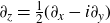 $\partial_z = \tfrac12 (\partial_x - i \partial_y)$
. Setting
 $\varPhi = f^{-1}f_z$
and
 $\overline \varPhi = \overline{f^{-1}f_z} = f^{-1}f_{\bar z}$
and
 $\beta = f^{-1} df = \varPhi dz + \overline \varPhi d \bar z$
, the Maurer–Cartan equation
 $d \beta + \frac{1}{2}\left[\beta \wedge \beta\right]=0$
and the second fundamental form of f can be rephrased as, see [Reference Dorfmeister, Inoguchi and Kobayashi8, section 1·1]
 \begin{equation} \varPhi_{\bar z} - \overline{\varPhi}_z + [\overline{\varPhi},\varPhi]=0 \quad\mbox{and}\quad \varPhi_{\bar z} + \overline{\varPhi}_z + \{\overline{\varPhi},\varPhi\}=e^{u} f^{-1} \boldsymbol{H},\end{equation}
where
 $e^u dz d \bar z$
and
 $\boldsymbol{H}$
denote the induced conformal metric and the mean curvature vector, respectively. Note that
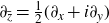 $\partial_{\bar z} = \tfrac12( \partial_x + i \partial_y)$
, and
 $u : \mathbb{D} \to \mathbb{R}$
is a real-valued function on
 $\mathbb{D}$
.
We now rephrase the fundamental equations in (3·1) in terms of generating spinors. Since f is a conformal immersion, it is easy to see that
 \begin{equation}\phi_1^2+ \phi_2^2 - \phi_3^2 =0\quad\mbox{and}\quad |\phi_1|^2 +|\phi_2|^2-|\phi_3|^2 = \frac{1}{2} e^u.\end{equation}
The generating spinors
 $\psi_1$
and
 $\psi_2$
are defined as a solution of
 $\phi_1^2+ \phi_2^2 - \phi_3^2 =0$
with
 \begin{equation*} \phi_1 = (\overline{\psi_2})^2 - \psi_1^2, \quad \phi_2 = i ((\overline{\psi_2})^2 + \psi_1^2), \quad \phi_3 = 2 i \psi_1 \overline{\psi_2}, \end{equation*}
where
 $\overline{\psi_2}$
denotes the complex conjugate of
 $\psi_2$
. Note that
 $\psi_1 \sqrt{d z}$
and
 $\overline{\psi_2} \sqrt{d z}$
are well defined on M.
The conformal factor
 $e^{u}$
of the induced metric
 $\langle df,df\rangle$
can be expressed by the spinors
 $\psi_1, \psi_2$
via the second formula at (3·2):
 \begin{equation*} e^{u} =4 (|\psi_1|^2-|\psi_2|^2)^2. \end{equation*}
In the following, we assume the regularity condition
 $|\psi_1|\neq|\psi_2|$
. A straightforward computation shows that
 \begin{equation} f^{-1} f_z \times f^{-1} f_{\bar z} = i e^{u/2} \left( 2 \Im (\psi_1 \psi_2 )e_1- 2 \Re (\psi_1 \psi_2)e_2- (|\psi_1|^2 + |\psi_2|^2)e_3\right). \end{equation}
Let us denote the unit normal vector field of f by N. From (3·3), N is given by
 \begin{equation} N=e^{-u/2}L, \quad \quad f^{-1} L = 2 \left( 2 \Im (\psi_1 \psi_2 )e_1- 2 \Re (\psi_1 \psi_2)e_2- (|\psi_1|^2 + |\psi_2|^2)e_3\right). \end{equation}
The support function h of f, with respect to z, (which is evidently non-vanishing for a spacelike surface) is defined as:
 \begin{equation} h := \langle f^{-1} L, e_3 \rangle = 2(|\psi_1|^2+|\psi_2|^2). \end{equation}
It is straightforward to check the following theorem, see [Reference Dorfmeister, Inoguchi and Kobayashi8, theorem 3·5] for the case of a surface in
 $\text{Nil}^{3}$
:
Theorem 3·1. The pair of generating spinors
 $\{\psi_1, \psi_2\}$
satisfies the following nonlinear Dirac equation,

where
 \begin{equation*} \mathcal U = \mathcal V = \frac{H}{2}e^{u/2}i - \frac{1}{4}h. \end{equation*}
Here H,
 $e^{u}$
and h are the mean curvature, the conformal factor and the support function for f respectively.
Moreover, together with the second fundamental form, the vector
 $\tilde \psi = (\psi_1, \psi_2)$
satisfies the following system
 \begin{equation}\tilde \psi_z = \tilde \psi \tilde U, \quad\tilde \psi_{\bar z}= \tilde \psi \tilde V,\end{equation}
where
 \begin{equation} \tilde U = \begin{pmatrix} \frac12 w_z - \frac{i}2 H_z e^{-w/2+u/2}&- e^{w/2} \\ B e^{-w/2}& 0 \end{pmatrix}, \quad \tilde V = \begin{pmatrix} 0 & - \bar B e^{-w/2} \\ e^{w/2}& \frac12 w_{\bar z} - \frac{i}2 H_{\bar z} e^{-w/2+u/2} \end{pmatrix}.\end{equation}
Here the function
 $e^{w/2}$
is the Dirac potential defined by

and the quadratic differential
 $B \, dz^2$
will be called the Abresch–Rosenberg differential given by
 \begin{equation*} B = \frac{2 i H + 1}{2}\left( \psi_1 \overline{\psi_2}_z - \overline{\psi_2} {\psi_1}_z \right) + 2i H (\psi_1\overline{\psi_2} )^2. \end{equation*}
The unit normal
 $f^{-1} N$
can be considered as a map into the the union of two hyperbolic two-spaces
 $\mathbb H^2_+ \cup \mathbb H^2_- \subset \mathbb E^3_1 (= \mathfrak{nil}^3_1)$
, where
 (resp.
 $\mathbb H^2_-$
) denotes the hyperbolic two-space with positive (resp. negative)
 $e_3$
-component. Note that when
 $|\psi_1|\gt|\psi_2|$
(resp.
 $|\psi_2|\gt|\psi_1|$
),
 $f^{-1}N$
takes values in
 $\mathbb H^2_-$
(resp.
 $\mathbb H^2_+$
). We now consider the normal Gauss map g of the surface f as a map defined as the composition of the stereographic projection
 $\pi$
from the point
 $(0, 0,-1)$
with
 $f^{-1} N$
in (3·4), that is,
 $g = \pi \circ f^{-1} N: \mathbb{D} \to \mathbb{C} \cup \{\infty\} \setminus \mathbb S^1$
, (here we identify (x, y, 0) with
 $ - y + i x$
) and thus, we obtain
 \begin{equation} g= \frac{\psi_1}{\overline{\psi_2}} \end{equation}
and
 $f^{-1}N$
can be represented by the normal Gauss map g as
 \begin{equation*} f^{-1} N = \frac1{|g|^2-1}\left( 2 \Im (g) e_1 - 2 \Re (g) e_2 - (|g|^2+1) e_3\right). \end{equation*}
We now introduce a family of Maurer–Cartan forms
 $\{\alpha^{\lambda}\}_{\lambda \in \mathbb S^1}$
:
 \begin{equation} \alpha^{\lambda} = U^{\lambda} d z + V^{\lambda} d \bar z, \end{equation}
where
 \begin{equation*} U^{\lambda} = \begin{pmatrix} \frac14 w_z - \frac{i}2 H_z e^{-w/2+u/2}&-\lambda^{-1} e^{w/2} \\ \lambda^{-1}B e^{-w/2}& -\frac14 w_z \end{pmatrix}, \quad V^{\lambda} =\begin{pmatrix} -\frac14 w_{\bar z} & - \lambda \bar B e^{-w/2} \\ \lambda e^{w/2}& \frac14 w_{\bar z} - \frac{i}2 H_{\bar z} e^{-w/2+u/2}\end{pmatrix}. \end{equation*}
Note that
 $U^{\lambda}|_ {\lambda =1}$
and
 $V^{\lambda}|_{\lambda =1}$
are obtained by a gauge transformation applied to
 $\tilde U$
and
 $\tilde V$
in (3·8), that is
 $\mathrm{Ad} (G^{-1}) (\tilde U) + G^{-1} G_z$
and
 $\mathrm{Ad} (G^{-1}) (\tilde V) + G^{-1} G_{\bar z}$
with the matrix
 $G = \mathrm{diag} (e^{-w/4}, e^{-w/4})$
. Then we characterise a spacelike maximal surface in
 ${\text{Nil}^{3}_{1}}$
in terms of the family of connections
 $d + \alpha^{\lambda}$
and the normal Gauss map g as follows.
Theorem 3·2. Let
 $f : \mathbb{D} \to {\text{Nil}^{3}_{1}}$
be a conformal spacelike immersion and
 $\alpha^{\lambda}$
the 1-form defined in (3·10) and g the normal Gauss map in (3·9). Then the following statements are mutually equivalent:
-
(i) f is a maximal surface;
-
(ii)
$d + \alpha^{\lambda}$
is a family of flat connections on
$\mathbb{D} \times SU(2)$
; -
(iii) The normal Gauss map g for f is a nowhere holomorphic harmonic map into the 2-sphere.


The proof is almost verbatim to the case of a surface in
 $\text{Nil}^{3}$
, see for example [Reference Dorfmeister, Inoguchi and Kobayashi8], thus we omit.
From theorem 3·2, there exists a family of maximal surfaces
 $\{f^{\lambda}\}_{\lambda \in \mathbb S^1}$
parameterised by
 $ \lambda \in \mathbb S^1$
with a pair of generating spinors
 $\{\psi_1 (\lambda ), \psi_2 (\lambda )\}$
such that
 $\{\psi_1 (\lambda), \psi_2 (\lambda)\}|_{\lambda =1}$
are the generating spinors of
 $f = f^{\lambda}|_{\lambda = 1}$
. Moreover, we can define a map F from
 $\mathbb{D} $
into SU(2) associated with respect to the generating spinors
 $\psi_1$
and
 $\psi_2$
for a maximal surface:
 \begin{equation} F(\lambda) =\frac{1}{\sqrt{|\psi_1(\lambda)|^2+|\psi_2(\lambda)|^2}}\begin{pmatrix} \psi_1(\lambda) & \psi_2(\lambda) \\ - \overline{\psi_2(\lambda)} & \overline{\psi_1(\lambda)}\end{pmatrix}. \end{equation}
Then F will be called the extended frame of the spacelike maximal surface and the harmonic normal Gauss map
 $g = \psi_1/\overline{\psi_2}$
.
Remark 3·3.
-
1. Without loss of generality
$F(\lambda)$
take values in
$\Lambda SU(2)_\sigma$
. -
2. It is easy to see that the Abresch–Rosenberg differential
$Bdz^2$
is holomorphic for any maximal surface. Moreover, it is holomorphic for any spacelike constant mean curvature surface. -
3. On the one hand, there are non-constant mean curvature surfaces which have the holomorphic Abresch–Rosenberg differential, the so-called Hopf cylinders.


Using a logarithmic derivative of the extended frame F with respect to
 $\lambda$
, we have a formula for a conformal maximal surface in
 ${\text{Nil}^{3}_{1}}$
. We now define a map
 \begin{equation*}\Xi_{\mathrm{nil}} = \mathrm{exp} \circ \Xi: \mathfrak{su}_2 \to {\text{Nil}^{3}_{1}}\end{equation*}
by the composition of a linear isomorphism
 $\Xi : \mathfrak {su}_2 \to \mathfrak h$
given by
 $\mathfrak{su}_2 \ni x_1 E_1 + x_2 E_2 + x_3 E_3 \mapsto x_1 e_1 + x_2 e_2 + x_3 e_3 \in \mathfrak h$
, where
 \begin{equation} E_1 :=\frac12 \begin{pmatrix}0 & -i \\ -i & 0 \end{pmatrix}, \quad E_2 :=\frac12 \begin{pmatrix}0 & 1 \\ -1 & 0 \end{pmatrix}, \quad E_3 := \frac{1}{2}\begin{pmatrix} i & 0\\0 &-i\end{pmatrix}, \end{equation}
and the exponential map
 $\mathrm{exp}: \mathfrak h \to {\text{Nil}^{3}_{1}}$
in (2·1).
Theorem 3·4. Let F be the extended frame for a spacelike maximal surface. Define maps
 $f_{cmc}$
and N respectively by
 \begin{equation} f_{cmc}=-i \lambda (\partial_{\lambda} F) F^{-1} -N \quad \mbox{and} \quad N= \mathrm{Ad} (F) E_3. \end{equation}
Moreover, define a map
 $f^{\lambda}:\mathbb{D}\to {\text{Nil}^{3}_{1}}$
by
 $f^{\lambda}:=\Xi_{\mathrm{nil}}\circ \hat{f^{\lambda}}$
with
 \begin{equation} \hat f^{\lambda} = \left. \left(f_{cmc}^o -\frac{i}{2} \lambda (\partial_{\lambda} f_{cmc})^d\right) \;\right|_{\lambda \in \mathbb{S}^1},\end{equation}
where the superscripts “o” and “d” denote the off-diagonal and diagonal part, respectively. Then, for each
 $\lambda \in \mathbb{S}^1$
, the map
 $f^{\lambda}$
is a maximal surface in
 ${\text{Nil}^{3}_{1}}$
and
 $ \pi \circ N$
is the normal Gauss map of
 $f^{\lambda}$
, where
 $\pi$
is the stereographic projection from the north pole. In particular,
 $f^{\lambda}|_{\lambda =1}$
gives the original spacelike maximal surface up to a rigid motion.
Proof. The proof is almost identical to that of [Reference Dorfmeister, Inoguchi and Kobayashi8, theorem 6·1]. In fact, we can compute the derivative of
 $f_{cmc}$
with respect to z:
 \begin{equation*} \partial_z f_{cmc} = \phi_1 E_1 + \phi_2 E_2 - i \phi_3 E_3, \end{equation*}
and a straightforward computation shows that
 \begin{equation*} \partial_z \hat f^{\lambda} = \phi_1 E_1 + \phi_2 E_2 + \left( \phi_3 - \frac12 \phi_1 \int \phi_2 dz + \frac12 \phi_2 \int \phi_1 dz \right) E_3\end{equation*}
holds. Finally, by the linear isomorphism
 $\Xi$
, we obtain
 \begin{equation*}(f^{\lambda})^{-1} \partial_z f^{\lambda} = \phi_1 e_1 + \phi_2 e_2 + \phi_3 e_3.\end{equation*}
Then the maximality of
 $f^{\lambda}$
follows immediately.
Remark 3·5.
-
1. Identifying the Lie algebra
${\mathfrak {su}}(2)$
with the Euclidean 3-space
$\mathbb{E}^3$
, with orthonormal basis in (3·12), the map
$f_{cmc}$
in (3·13) defines a constant mean curvature surface with
$H_{cmc} =1/2$
in
$\mathbb{E}^3$
, see for example [Reference Bobenko2]. The formula above for
$f_{cmc}$
corresponds to the choice
$f^-$
in section 1·2. The Gauss map g used here is holomorphic exactly when either
$N_x = N \times N_y$
, or
$N_z =0$
, i.e., when the map
$f^-$
fails to be regular. So
$f_{cmc}$
is regular for a nowhere holomorphic harmonic map. -
2. It is known that for a given nowhere holomorphic harmonic map g from a surface M into
$\mathbb S^2$
, there exists a regular constant mean curvature
$H_{cmc} \neq 0$
surface in the Euclidean 3-space, [Reference Kenmotsu15]. In particular, the induced metric of the surface is given by Moreover, there exists an extended frame F corresponding to the nowhere holomorphic harmonic map g and the CMC surface, see theorem 3·2 and thus one can define a map map
\begin{equation*} ds^2 = \left(\frac2{H_{cmc}} \frac{| \partial_{\bar z} g|}{1 + |g|^2} \right)^2|dz|^2. \end{equation*}
$f^{\lambda}$
by (3·14).


3·2. Generalised maximal surfaces
We first give an alternative proof of a result that can be found in [Reference Lee18]:
Theorem 3·6. There does not exist any complete spacelike maximal surface in
 ${\text{Nil}^{3}_{1}}$
.
Proof. From the construction in theorem 3·4, for a spacelike maximal surface f in
 ${\text{Nil}^{3}_{1}}$
, there exists a corresponding CMC surface
 $f_{cmc}$
in the Euclidean 3-space. The metric of the CMC surface is given by
 $ds_e^2 = h^2 dz d \bar z$
, where h is the support function defined in (3·5). Then it is easy to see that the induced metric
 $ds^2 = e^{u}d z d \bar z$
of the spacelike maximal surface and the induced metric
 $ds_e^2$
of the corresponding CMC surface have the following relation:
 \begin{equation} e^{u} + 4 |\phi_3|^2 = h^2. \end{equation}
Therefore completeness of the metric
 $ds^2$
implies completeness of the metric
 $ds_{e}^{2}$
. Moreover, the Gauss map of the maximal surface always takes values eithre in
 $\mathbb H^{2}_{+}$
or
 $\mathbb H^{2}_{-}$
. This implies that the corresponding normal Gauss map (through the stereographic projection to the unit disk
 $\mathbb{D}$
or the outside of the unit disk
 $\mathbb{C} \cup \{\infty\} \setminus \bar{\mathbb{D}}$
) of the corresponding CMC surface takes values in the upper open hemisphere or the lower open hemisphere. But according to [Reference Hoffman, Osserman and Schoen13, theorem 1], there is no complete non-minimal CMC surface that has Gauss image contained in a hemisphere.
From theorem 3·4, it is natural to consider spacelike maximal surfaces in
 ${\text{Nil}^{3}_{1}}$
with singularities. Since the normal Gauss map
 $g = \psi_1/\overline{\psi_2}$
is a harmonic map into
 $\mathbb{C} \cup \{\infty\}$
minus
 $\mathbb S^1$
, it satisfies the elliptic PDE:
 \begin{equation} g_{z \bar z} - \frac{2\bar g}{1+|g|^2} g_{\bar z} g_z=0. \end{equation}
By using the nonlinear Dirac equation in (3·6), we compute
 $ \bar g_{z} = - \frac12 (\overline \psi_2)^2 (|g|^2+1)^2$
, which, by setting
 $\omega = i \, \overline{\psi_2}^2$
, is equivalent to
 \begin{equation} \omega = -\frac{2i\bar g_{z}}{(|g|^2+1)^2}. \end{equation}
Moreover, by the equation in (3·7) we have
 \begin{equation} \frac{i }{2}g_z \omega = \frac{g_{z} \bar g_{z}}{(|g|^2+1)^2}= B. \end{equation}
The induced metric
 $ds^2 =4 (|\psi_1|^2- |\psi_2|^2)^2 |dz|^2$
of a maximal surface in
 ${\text{Nil}^{3}_{1}}$
is written in terms of g and
 $\omega$
as
 \begin{equation} ds^2 = (1-|g|^2)^2 |\omega|^2 |dz|^2 = 4|\bar g_{z}|^2\frac{(1-|g|^2)^2}{(1+|g|^2)^4} |dz|^2. \end{equation}
Therefore, there are two possibilities to generalise maximal surfaces in
 ${\text{Nil}^{3}_{1}}$
as
 \begin{equation*} |g|^2 =1 \quad \mbox{or} \quad g_{\bar z} =0 \end{equation*}
at
 $p \in M$
. From the harmonic map point of view, it is natural to consider a harmonic map into
 $\mathbb{C} \cup \{\infty\}$
. The latter case, the
 $g_{\bar z}(p)=0$
, is equivalent to that the harmonic map g is holomorphic at point p. It turns out that in the proof of theorem 4·1 a holomorphic point is always a degenerate singular point. Therefore we will, generally speaking, exclude such points.
On the other hand, from a nowhere holomorphic harmonic map from a Riemann surface into
 $\mathbb{C} \cup \{\infty\}$
, we can define the generating spinors
 $\psi_1, \psi_2$
by (3·17) and
 $g = \psi_1/\overline{\psi_2}$
. Then one can introduce the extended frame
 $F(\lambda)$
as in (3·11) and the Sym-formula
 $f = f^{\lambda}|_{\lambda=1}$
defined by in (3·14). Then it is clear that the map f defines a maximal surface where it has a regular point, that is
 $|g|^2 \neq 1$
. It is natural to define the following class of surfaces.
Definition 3·7 (Generalised spacelike maximal surfaces). Let g be a nowhere holomorphic harmonic map from a Riemann surface M into
 $\mathbb{C} \cup \{\infty\}$
, and a map f into
 ${\text{Nil}^{3}_{1}}$
as defined above. Then f will be called a generalised spacelike maximal surface in
 ${\text{Nil}^{3}_{1}}$
, and g will be called the normalised Gauss map of f.
Remark 3·8.
-
(1) For each
$\lambda \in \mathbb S^1$
,
$f^{\lambda}|_{\lambda \in \mathbb S^1}$
is also a generalised spacelike maximal surface. -
(2) In general, a rotation of a nowhere holomorphic harmonic map g as a map on the 2-sphere changes the corresponding generalised maximal surface completely; a rotation around the
$e_3$
-axis g gives an isometry of the surface in
${\text{Nil}^{3}_{1}}$
but other rotations do not give isometries. Thus in Definition 3·7 we choose g with some fixed initial condition and choose the extended frame F which gives
$\pi \circ N = g$
with
$N = \mathrm{Ad}_F E_3|_{\lambda=1}$
.



3·3. Numeric examples
An extended frame for any harmonic map into
 $\mathbb{S}^2$
, and hence any maximal surface in
 ${\text{Nil}^{3}_{1}}$
, can be constructed via the method of Dorfmeister-Pedit-Wu (DPW) [Reference Dorfmeister, Pedit and Wu9], from a holomorphic potential of the form:
 \begin{equation*}\xi = \sum_{n=-1}^\infty A_n(z) \lambda^n \textrm{d} z.\end{equation*}
Solving the ODE
 $\Phi_z = \Phi \xi$
, with an initial condition
 $\Phi(z_0) = I$
, gives a so-called complex extended frame, and an extended frame F for a harmonic map is then obtained from
 $\Phi$
by a pointwise Iwasawa decomposition
 $F = \Phi B_+$
, where
 $B_+$
extends holomorphically, in the parameter
 $\lambda$
, to the unit disc. To produce a nowhere holomorphic harmonic map g, or equivalently, a regular CMC surface
 $f_{cmc}$
we need the regularity condition:
 \begin{equation} (A_{-1})_{1,2} \neq 0, \end{equation}
which corresponds to the function
 $e^{w/2}$
in
 $U^\lambda$
being non-zero.
Potentials corresponding to various geometric properties for CMC surfaces have been found in numerous subsequent works, and the solutions can be computed numerically.
A major difference when using this method for maximal surfaces in the Heisenberg group is that the action of the group SU(2) is not an isometry. Pre-multiplying an extended frame by an element of SU(2) will result in an extended frame for a geometrically distinct solution. Therefore, for a given potential, many different solutions are obtained, depending on the initial condition.
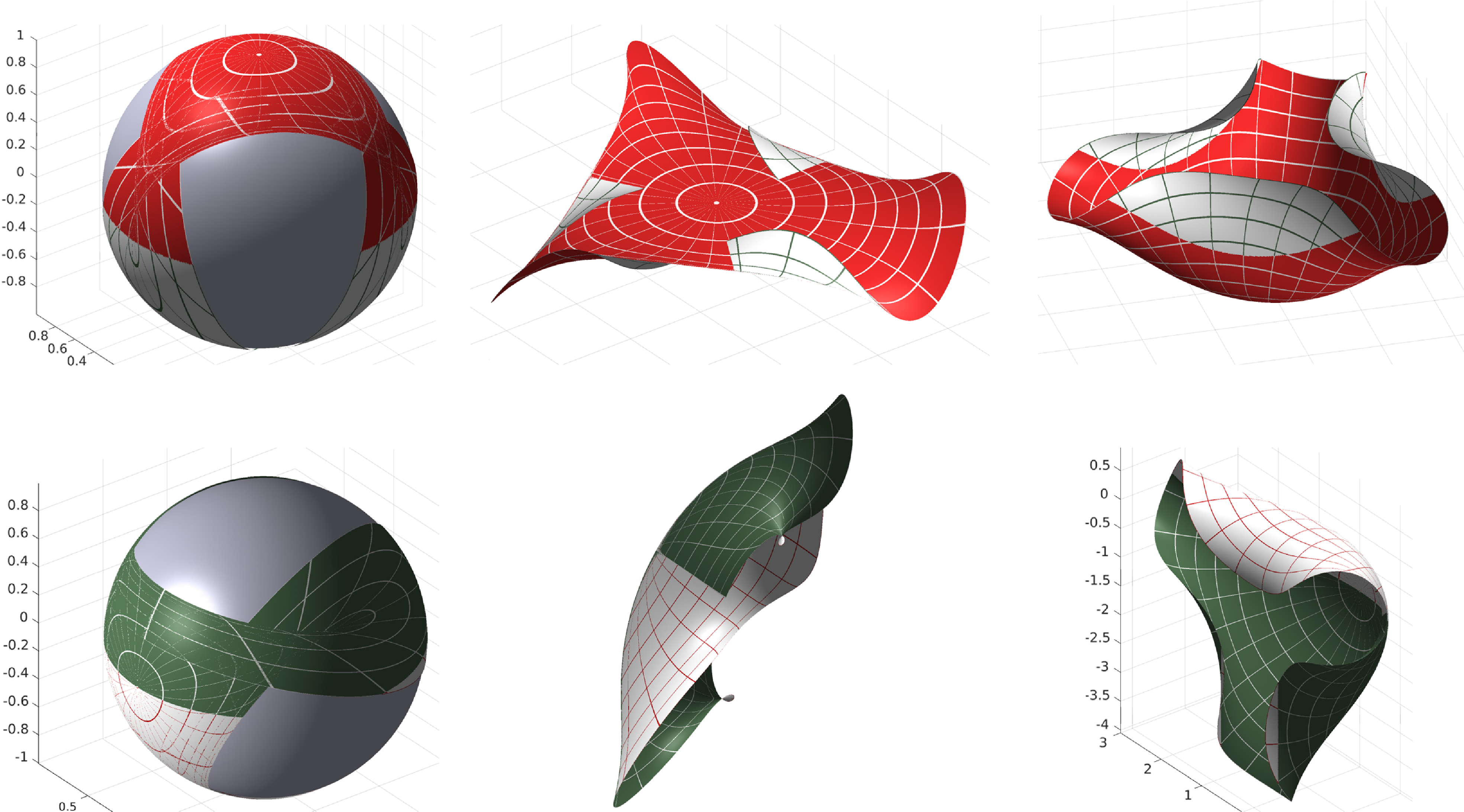
Interpreting the images. In Figures 1 and 2, the surfaces are oriented with the
 $e_3$
-axis directed upwards, and are coloured according to whether the harmonic map takes values in the upper or lower hemisphere. Since the singular set corresponds to the equator separating these two hemispheres, the plot of the maximal surface in
 ${\text{Nil}^{3}_{1}}$
changes colour at the singular set. The plot can, of course, appear to change colour at a place where the surface has a self intersection, for example the lower middle image in Figure 2.
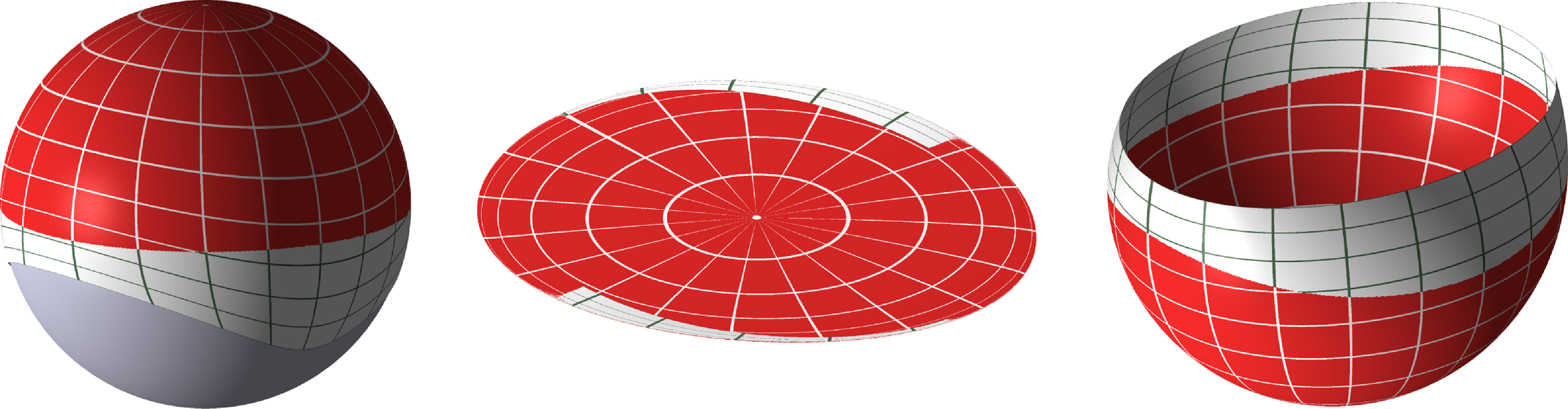
The solutions of Example 3·10. Left: harmonic maps; middle: corresponding maximal surface in
 ${\text{Nil}^{3}_{1}}$
; right: corresponding CMC surfaces in Euclidean space.

Example 3·9. As is well known, a CMC surface of revolution in
 $\mathbb{R}^3$
is obtained from a potential of the form:
 \begin{equation*} \xi(z) = \begin{pmatrix} 0 & -a\lambda^{-1}+(a-1)\lambda \\ (1-a)\lambda^{-1} + a\lambda & 0 \end{pmatrix} \textrm{d} z. \end{equation*}
The case
 $a=1.2$
is computed and plotted in Figure 1. The CMC surface is a nodoid. On the second row we show examples of the diferent maximal surfaces in
 ${\text{Nil}^{3}_{1}}$
obtained by choosing a different axis of symmetry for the nodoid. The harmonic Gauss map of the nodoid is doubly periodic. In the figure, for each case, the singular set for the lower surface coresponds to where the normal to the CMC surface above is perpendicular to the
 $E_3$
-direction. At such points, if the Gauss map is symmetric about the equator, then a fold singularity is created on the maximal surface (first two examples).
Example 3·10. CMC surfaces with rotationally symmetric metric can be constructed via the potential:
 \begin{equation*} \xi(z) = \begin{pmatrix} 0 & 1 \\ z^k & 0 \end{pmatrix} \lambda^{-1} \textrm{d} z, \end{equation*}
where k is a positive integer. For the case
 $k=1$
, in Figure 2 we display a local solution with two different initial conditions for the SU(2)-frame.
Since SU(2) acts by isometries on
 $\mathbb{S}^2$
and
 $\mathbb{R}^3$
, the harmonic map and the CMC surface are unchanged (up to isometry) regardless of the initial condition, but the maximal surface in
 ${\text{Nil}^{3}_{1}}$
is different. When the
 $e_3$
axis is chosen as the axis of symmetry for the harmonic map (top row in Figure 2), the maximal surface has an order 3 rotational symmetry about the
 $e_3$
-axis, and has three cuspidal cross-cap singularities within the domain. When one of the other axes is chosen as the axis of symmetry for N (bottom row), the corresponding maximal surface is no longer symmetric and has only one cuspidal cross-cap singularity in the domain, at the center.
Example 3·11. Potentials of the form
 \begin{equation*}\xi(z) = \begin{pmatrix} 0 & a(z) \\ b(z) & 0 \end{pmatrix} \lambda^{-1} \textrm{d} z,\end{equation*}
where a(z) and b(z) are meromorphic are called normalised potentials. If integrated with initial condition
 $\Phi(z_0)=I$
, then
 $z_0$
is called the normalisation point. In [Reference Brander and Dorfmeister4], it is shown (lemma 7·3) that a CMC surface has a dihedral rotational symmetry of order n about the normalisation point
 $z=0$
if and only if the meromorphic functions a and b have Laurent expansions of the form:
 \begin{equation*}a(z) = \sum_j a_{nj} z^{nj}, \quad \quad b(z) = \sum_j b_{nj-2} z^{nj-2}.\end{equation*}
(Thus the CMC surface in Example 3·10 also has a dihedral symmetry of order
 $k+2$
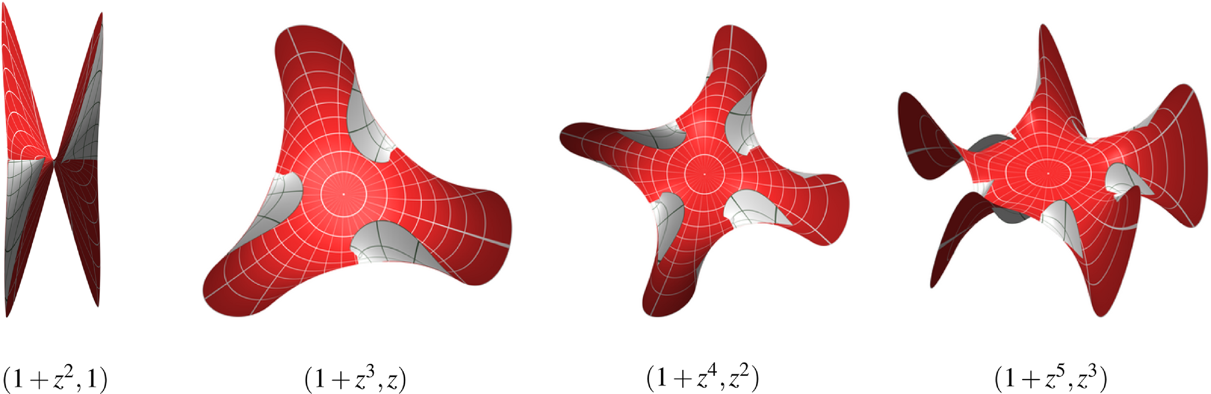
). Examples are computed and shown in Figure 3, where the initial condition is chosen so that the
 $e_3$
-axis is perpendicular to the tangent plane at the point of symmetry. Thus the maximal surface also has the dihedral symmetry. For these cases, the order n symmetric examples apparently have n cuspidal cross-cap singularities in the domain computed (a disc around
 $z=0$
). The corresponding constant positive Gauss curvature surfaces can be found in [Reference Brander3, figure 4].
Maximal surfaces with rotational symmetry (Example 3·11), computed from normalised potentials with the displayed functions (a(z),b(z)).

Top: CMC
 $1/2$
surfaces in
 $\mathbb{E}^3$
. Bottom: the corresponding maximal surfaces in
 ${\text{Nil}^{3}_{1}}$
, with, in order, cuspidal edge, swallowtail, and cuspidal cross-cap singularities. (Example 4·8).

4. Generic singularities for maximal surfaces in
${{\rm Nil}^{3}_{1}}$

Generalised surface such as those studied here, where there is a well defined normal map even at points where the surface is not immersed, are called frontals (see, e.g. [Reference Ishikawa14]). It is of interest to classify the generic singularities of frontals for a given surface type. The classification is done at the level of germs and up to differential equivalence, that is up diffeomorphisms on the source and target. The generic singularity criteria for spacelike maximal faces in Minkowski space
 $\mathbb L^3$
has been given in [Reference Umehara and Yamada23, theorem 3·1], see also the definition of “maximal faces” there and in [Reference Fujimori, Saji, Umehara and Yamada12, theorem 2·4]. The generic singularities are called cuspidal edge, cuspidal cross-cap and swallowtail. All of these singularities correspond to a curve
 $\gamma$
in the coordinate space, called the singular curve. The generic singularities are characterised by the behaviour of the normal along the singular curve. The main ingredients needed, and which we will compute below, are the singular curve, the Euclidean normal, and the 1-dimensional vector bundle defined by its kernel along the singular curve. Below we will first give criteria for three standard singularities for maximal surfaces in
 ${\text{Nil}^{3}_{1}}$
, and then show that these are the generic ones.
4·1. Characterisation of standard singularities
Theorem 4·1 (Singularity criteria). Let g be the normal Gauss map of a generalised spacelike maximal surface f in
 ${\text{Nil}^{3}_{1}}$
. Then the singular points of f are given by
 $|g|^2 =1$
and f is degenerate at a singular point p if and only if
 \begin{equation*}\Re \left[\frac{g^{\prime}}{g^2 \omega }\right] = \Im \left[\frac{g^{\prime}}{g^2 \omega}\right] +2 =0,\end{equation*}
where
 $\prime=\partial_z$
and the function
 $\omega$
is defined by (3·17), i.e.,
 $\omega = -(2i\bar g_{z})/(|g|^2+1)^2$
. Moreover, f is a wave front at a singular point p if and only if
 $\Re (g^{\prime}/(g^2 \omega)) \neq 0$
, and the following criteria hold
 $:$
-
(i) f is
$\mathcal A$
-equivalent to a cuspidal edge at p if and only if
\begin{equation*} \Re \left[ \frac{g^{\prime}}{g^2 \omega}\right] \neq 0 \quad \mbox{and}\quad \Im \left[ \frac{g^{\prime}}{g^2 \omega}\right] \neq -2; \end{equation*}
-
(ii) f is
$\mathcal A$
-equivalent to a swallowtail at p if and only if
\begin{equation*} \frac{g^{\prime}}{g^2\omega} + 2 i \in \mathbb R^{\times}\quad \mbox{and}\quad \Im \left[\frac1{(\log |g|)^{\prime}}\left(\Im \left(\frac{g^{\prime}}{g^2 \omega}\right)\right)^{\prime} \right] \neq 0; \end{equation*}
-
(iii) f is
$\mathcal A$
-equivalent to a cuspidal cross-cap at p if and only if
\begin{equation*} \frac{g^{\prime}}{g^2\omega} + 2 i \in i \mathbb R^{\times} \quad \mbox{and}\quad \Re \left[\frac1{(\log |g|)^{\prime}}\left(\Im \left(\frac{g^{\prime}}{g^2 \omega}\right)\right)^{\prime} \right] \neq 0. \end{equation*}


Proof. Since the induced metric is given by (3·19), it is easy to see that f has a singular point at p if
 $|g|^2=1$
. Moreover, around a point p where
 $g(p) = \infty$
the induced metric can be computed as
 \begin{equation*} ds^2 =4|\bar g_{z}|^2\frac{(1-|g|^2)^2}{(1+|g|^2)^4} |dz|^2 = 4|\bar {\hat g}_{z}|^2\frac{(1-|\hat g|^2)^2}{(1+|\hat g|^2)^4} |dz|^2, \end{equation*}
where
 $\hat g = 1/g$
. The normal Gauss map is nowhere holomorphic and thus the induced metric at the point
 $g(p) = \infty$
is regular. Thus the first claim follows.
The Euclidean cross product
 $\times_{e}$
of
 $f^{-1}f_x$
and
 $f^{-1}f_y$
, where
 $z = x + iy$
, is given by
 \begin{align*}f^{-1}f_x \times_{e} f^{-1}f_y &= -2 i f^{-1}f_{z} \times_{e} f^{-1}f_{\bar z} \\ &= |\omega|^2 (|g|^2 - 1)\left( 2 \Im (g )e_1- 2 \Re (g)e_2 + (|g|^2 + 1)e_3\right),\end{align*}
where
 $\omega = -(2i\bar g_{z})/(|g|^2+1)^2$
as before. Note that at a singular point we have,
 $\omega (p) =- i \bar g_{z}(p)/2 \neq 0$
. Then the Euclidean unit normal
 $f^{-1} N_{e}$
is computed by
 \begin{equation*}f^{-1} N_{e} = \frac1{\sqrt{(1+|g|^2)^2 + 4 |g|^2}}\, \left(2 \Im(g) e_1 -2 \Re(g)e_2 + (1+|g|^2)e_3\right).\end{equation*}
Thus the function
 $\rho$
defined by
 $f^{-1}f_x \times_e f^{-1}f_y = \rho f^{-1} N_e$
is given by
 \begin{equation*} \rho = (|g|^2-1) |\omega|^2 \sqrt{(1+|g|^2)^2 + 4 |g|^2}.\end{equation*}
A singular point
 $p \in M$
is called non-degenerate if
 $d \rho$
does not vanish at p (see [Reference Umehara and Yamada23]) and otherwise called degenerate. It is easy to see by using
 $|g|^2 =1$
that
 \begin{equation*} \textrm{d} \rho (p) = 2 \sqrt{2} |\omega|^2 \left(\frac{\textrm{d} g}{g} + \frac{\textrm{d} \bar g}{\bar g}\right).\end{equation*}
Since
 $\omega= - i \bar g_{z}(p)/2$
is assumed non-vanishing,
 $\textrm{d} \rho(p)$
vanishes if and only if
 $(\textrm{d} g/g + \textrm{d} \bar g/\bar g$
vanishes, which is equivalent to
 $g'/(g^2 \bar g') + 1 =0$
. Therefore f is degenerate at a singular point p if and only if
 \begin{equation*} \Im (g^{\prime}/(g^2 \bar g^{\prime} )) = \Re (g^{\prime}/(g^2 \bar g^{\prime})) + 1 =0, \end{equation*}
which is equivalent to the first conditions.
Next using g and
 $\omega$
at a singular point p, that is
 $|g(p)|^2=1$
or
 $\bar g(p) = 1/g(p)$
, we have
 \begin{equation*}f^{-1} d f =(g \omega \textrm{d} z + \bar g \bar \omega \textrm{d} \bar z) (\Im (g) e_1 - \Re (g)e_2 - e_3).\end{equation*}
Thus
 $\eta = i/(g \omega)$
is the null-direction of df at p. A straightforward computation shows that
 \begin{equation*}d N_e (p) = -\frac{i}{2\sqrt{2}} \left(\frac{d g}{g}- \frac{d \bar g}{\bar g}\right)(\Re(g), \Im(g), 0).\end{equation*}
Then the null-direction of
 $d N_e$
at p is proportional to
 \begin{equation*} \mu = \overline{\left( \frac{g_z}{g}\right)}-\frac{g_{\bar z}}{g}.\end{equation*}
It is known that f is a wave front [Reference Kokubu, Rossman, Saji, Umehara and Yamada17] if and only if
 $\det (\mu, \eta) \neq 0$
, that is,
 \begin{equation*}\det (\mu, \eta)= \Im (\bar \mu \eta) = \Re \left\{\left( \frac{g_z}{g}-\frac{\bar g_{z}}{\bar g}\right) \frac{1}{g \omega}\right\}\neq0.\end{equation*}
Plugging the expression in (3·17) into this, we have the criterion for a wave front. We now assume that f is a wave front at p, that is,
 $\Re ( g_z/(g^2 \omega) )\neq 0$
at a singular point p. Then the singular curve
 $\gamma(t)$
with
 $\gamma(0)=p$
satisfies
 $g(\gamma(t)) \overline{g(\gamma(t))}=1$
, and thus
 \begin{equation*}\Re \left( \frac{g_{z}}{g} \dot \gamma + \frac{g_{\bar z}}{g} \dot {\bar \gamma} \right) = 0\end{equation*}
on the singular curve
 $\gamma (t)$
. Then without loss of generality,
 $\dot \gamma$
is given by
 \begin{equation}\dot \gamma(t)= i \left(\overline{\left(\frac{g_{z}}{g}\right)} + \frac{g_{\bar z}}{g}\right)(\gamma(t)).\end{equation}
Then using the criterion in [Reference Kokubu, Rossman, Saji, Umehara and Yamada17, Proposition 1·3 (1)], f has a cuspidal edge at p if and only if
 \begin{equation*}\det (\dot \gamma, \eta)|_{t=0}= \Im (\dot{\bar \gamma} \eta )= \Im \left(\frac{g_z}{g^2 \omega} + i \frac{(|g|^2+1)^2}{2 |g|^2}\right)= \Im \left(\frac{g_z}{g^2 \omega}\right)+2 \neq 0,\end{equation*}
where we use
 $|g|^2=1$
. Now the relation
 $\omega(p) = -i \bar g_{z} (p)/2$
implies the conclusion.
We now assume
 $\Re ( g_z/(g^2 \omega) )\neq 0$
and
 $\Im \left(g_z/(g^2 \omega)\right)= -2$
. Then using the criterion in [Reference Kokubu, Rossman, Saji, Umehara and Yamada17, Proposition 1·3 (2)], f has a swallowtail at p if and only if
 \begin{equation*} \frac{d \det (\dot \gamma, \eta)}{dt}\Big|_{t=0} \neq 0. \end{equation*}
Then a straightforward computation by using a relation
 $\frac{d}{dt}|_{t=0} (|g|^2+1)^2|g|^{-2}=0$
on
 $|g|=1$
shows that
 \begin{equation*} \frac{d \det (\dot \gamma, \eta)}{dt}\Big|_{t=0} = \Im \left\{\left(\frac{g_z}{g^2 \omega}\right)_z \dot \gamma + \left(\frac{g_z}{g^2 \omega}\right)_{\bar z} \dot {\bar\gamma} \right\}. \end{equation*}
Inserting the expressions in (4·1) into the above equation, we have the second criterion.
Finally we consider a criterion for cuspidal cross-caps. It is known that [Reference Fujimori, Saji, Umehara and Yamada12, corollary 1·5], f at
 $p = \gamma (0)$
is
 $\mathcal A$
-equivalent to a cuspidal cross-cap if and only if:
-
1.
$\eta (0)$
is transversal to
$\dot \gamma(0)$
; -
2.
$\chi (0) =0$
and
$\dot \chi (0)\neq 0$
.


Here
 $\chi$
is defined by (see the proof of [Reference Fujimori, Saji, Umehara and Yamada12, theorem 2·4])
 \begin{equation*} \chi = \det (f_* \dot \gamma, d N_e (\eta), N_e). \end{equation*}
It is easy to verify that condition (1) can be computed by
 \begin{equation*} \det (\dot \gamma, \eta) = \Im (\overline{\dot \gamma} \eta) = \Im \left(\frac{g_z}{g^2 \omega}\right)+2 \neq 0\end{equation*}
at p. Then the function
 $\chi$
can be computed as
 \begin{equation*} \chi = \Re \left( \frac{g^{\prime}}{g^2 \omega}\right) \chi_0, \end{equation*}
where
 $\chi_0$
is a smooth function and it is non-vanishing at p. Thus condition (2) can be computed by
 \begin{equation*}\Re \left( \frac{g^{\prime}}{g^2 \omega}\right) = 0, \quad\Re \left\{\left(\frac{g_z}{g^2 \omega}\right)_z \dot \gamma + \left(\frac{g_z}{g^2 \omega}\right)_{\bar z} \dot {\bar\gamma} \right\} \neq 0 .\end{equation*}
Inserting the expressions in (4·1) into the above equation, we have the third criterion.
Remark 4·2. The normal Gauss map g for a generalised spacelike maximal surface in
 ${\text{Nil}^{3}_{1}}$
is nowhere holomorphic harmonic, that is
 $g_{\bar z}$
is never zero. Therefore, the criteria in theorem 4·1 is different from that in [Reference Umehara and Yamada23, theorem 3·1] and in [Reference Fujimori, Saji, Umehara and Yamada12, theorem 2·4], where the normal Gauss map g was holomorphic.
4·2. A simplified characterisation
We now want to simplify the criteria in theorem 4·1 using a normalisation of the normal Gauss map g at a singular point. First we observe:
Lemma 4·3. Let g be the normal Gauss map of a generalised spacelike maximal surface, and
 $\omega = -2i\bar g_z/(|g|^2+1)^2$
. At a non-holomorphic singular point we can choose a coordinate z such that
 $:$
 \begin{equation} \textrm{d} (g \omega)(p) =0, \quad \quad \quad (g\omega)(p) = 1. \end{equation}
Proof. Using the harmonic map equation (3·16) we obtain:
 \begin{equation*} \textrm{d} (g \omega)(p) =\frac{i}{2}g\left(\bar g_{z \bar z} - g \bar g^2_z\right) \textrm{d} z. \end{equation*}
Since
 $\omega$
depends on the choice of coordinates, we can in fact choose coordinates to make the above expression zero. The new coordinate
 $\zeta$
is found by solving the equation
 $\textrm{d}^2 z/\textrm{d} \zeta^2 + C (\textrm{d} z/\textrm{d} \zeta)^2 = 0$
, where C is the value at p of
 $(\bar g_{zz}+g(\bar g_z)^2)/\bar g_z$
. Since
 $(g \omega)(p) \ne 0$
, a constant scaling of the coordinate finishes the proof.
Recall that by (3·18), the Abresch–Rosenberg differential
 $B \, \textrm{d} z^2$
, the normal Gauss map g, and the function
 $\omega$
have the following relation
 \begin{equation*} \frac{i}{2}g_z \omega = B. \end{equation*}
Putting these expressions into theorem 4·1 results in the following simplified statement:
Theorem 4·4. Let g be a normal Gauss map of a generalised maximal surface f in
 ${\text{Nil}^{3}_{1}}$
, with coordinates chosen as in lemma 4·3 at a singular point p. Then the singular point is degenerate if and only if
 \begin{equation*} \Im \left( B\right) = 0 \quad \text{and} \quad \Re \left(B\right) =1 \end{equation*}
at p, and f is a wave front at p if and only if
 $\Im (B) \neq 0$
. Moreover, writing
 $\prime = \partial_z$
, f is
 $\mathcal A$
-equivalent at p to a
 $:$
-
(i) cuspidal edge if and only if
$\Re (B) \neq 1$
and
$\Im (B) \neq 0$
$;$
-
(ii) swallowtail if and only if
$\Re (B) = 1$
and
$\Im (B) \neq 0$
and
$\Im \left(B^{\prime}\right) \neq 0$
$;$
-
(iii) cuspidal cross-cap if and only if
$\Re (B) \neq 1$
,
$\Im (B) = 0$
and
$\Im \left(B^{\prime}\right) \neq 0$
.


Remark 4·5. Vanishing of the derivative
 $h_z$
of the support function at a singular point is related to the vanishing of
 $(g\omega)_z$
. In fact the support function h can be rephrased as
 \begin{equation*} h^2 = 4 |\omega|^2(1+|g|^2)^2, \end{equation*}
and a straightforward computation, using the relations
 $|g(p)|^2=1$
and
 $(g\omega)_{\bar z}(p)=0$
at a singular point p, implies that
 $h_z(p)=0$
is equivalent to
 $(g\omega)_z(p)=0$
.
4·3. A construction of singularities through the DPW representation
We now show how to obtain these singularities via the DPW method described in section 3·3. A general holomorphic potential for the DPW method is of the form:
 \begin{equation} \xi(z) = \sum_{n=-1}^\infty \xi_i(z) \lambda^i \textrm{d} z,\end{equation}
where
 $\xi_i$
is holomorphic and takes values in
 $\mathfrak{sl}(2,\mathbb{C})$
, and is diagonal for even values of i and off-diagonal for odd. If
 $\xi$
satisfies the regularity condition (3·20), we can write:
 \begin{equation}\xi_{-1} := \begin{pmatrix} 0 & a(z) \\ b(z) & 0 \end{pmatrix}, \quad a(0) \neq 0,\quad B(z) := -b(z)a(z).\end{equation}
We now want to construct a generalised maximal spacelike surface in
 ${\text{Nil}^{3}_{1}}$
which has a singularity at p. Let C be a solution of
 $d C = C \tilde \xi$
taking values in
 $\Lambda SL(2, \mathbb C)_{\sigma} $
and choose an initial condition
 \begin{equation} C(p, \lambda) = C_0:= \frac1{\sqrt{2}} \begin{pmatrix} e^{i c} & i e^{i c} \lambda \\ i e^{-i c}\lambda^{-1}& e^{-i c} \end{pmatrix}\in \Lambda SU(2)_\sigma, \quad c \in \mathbb R,\end{equation}
that is, at p the Iwasawa decomposition is trivial
 $C(p, \lambda) = F(p, \lambda)$
and
 $V_+(p, \lambda) = \mathrm{id}$
. Note that the support h in (3·5) can be computed by
 $h = 4 v_0^2$
, where
 $v_0 $
is the leading term of (1,1)- of the expansion of
 $V_+(\lambda)$
with respect to
 $\lambda$
. Thus
 $h(p)= 4$
by
 $v_0(p)=1$
. Since
 $i g \omega = - \psi_1 \overline{\psi_2},$
(
 $g = \psi_1/\overline{\psi_2}, \omega = i \overline{\psi_2}^2$
) is given by the product of the half-support
 $h/2$
with h, (1,1)- and (2,1)- of F in (3·11), the map
 $g \omega$
takes value 1 at p and we have:
Theorem 4·6. Let
 $\xi$
be the potential given by (4·4) and C be the solution of
 $d C = C \xi$
with initial condition (4·5). Then the resulting generalised spacelike maximal surface f in
 ${\text{Nil}^{3}_{1}}$
through the DPW method has a singular point at
 $p({=}\,0) \in \mathbb{D}$
and the quadratic differential
 $B \, dz^2$
in (4·4) becomes the Abresch–Rosenberg differential for f.
Proof. From the standard procedure of the DPW method, an extended frame F which takes values in
 $\Lambda SU(2)_\sigma$
can be constructed by the Iwasawa decomposition of C, that is
 $C = F B_+$
, where C is the solution of
 $\textrm{d} C = C \xi$
with the initial condition
 $C(0)=C_0$
. Note that
 $B_+$
takes values in
 $\Lambda^{+} SL(2, \mathbb C)_{\sigma} $
. Since the initial condition takes values in
 $\Lambda SU(2)_\sigma$
, thus the
 $B_+$
is identity at
 $p=0$
and thus
 $C_0= F$
at 0. Thus the Gauss map g is i at 0 and therefore the resulting surface f has a singular point at 0. Then a direct computation shows that
 \begin{equation*} F^{-1} F_{z} = B_+ (\xi/\textrm{d} z) B_+^{-1} - B_{+ z} B_+^{-1} \end{equation*}
holds. Comparing it to
 $U^{\lambda}$
in (3·10), B(z) in the potential in (4·4) is the coefficient function of the Abresch–Rosenberg differential.
We cannot immediately apply the criteria of theorem 4·4 to B(z) for an arbitrary potential, because we also need the normalisation conditions (4·2) to hold. In fact any harmonic map can be represented by a normalised potential
 $\xi = {\tiny{\begin{pmatrix} 0 & a(z) \\ b(z) & 0 \end{pmatrix}}} \lambda^{-1} \textrm{d} z$
, as in Example 3·11. After a change of coordinate
 $\int_0^z a(w) \textrm{d} w$
, these are included in:
Corollary 4·7. Any holomorphic potential of the form
 $:$
 \begin{equation} \xi =\begin{pmatrix} 0 & 1 \\- B(z) & 0\end{pmatrix} \lambda^{-1} \textrm{d} z + \sum_{n=1}^\infty \xi_i(z) \lambda^i \textrm{d} z\end{equation}
satisfies the normalisation given in (4·2). The maximal surface f obtained by integrating
 $\xi$
with the initial condition (4·5) has a singularity at the point
 $z=0$
, and the singularity criteria in theorem 4·4 can be applied to the coefficient function B(z).
Proof. From theorem 4·6, f has a singular point at 0. Let C be the solution of
 $\textrm{d} C = C \xi$
with the initial condition (4·5) and consider the Birkhoff decomposition of C as
 \begin{equation*}C = C_- C_+,\end{equation*}
where
 $C_- \in \Lambda_{*}^{-} SL(2, \mathbb C)_{\sigma} , C_+ \in \Lambda^{+} SL(2, \mathbb C)_{\sigma} $
. Then
 $C_-$
gives
 \begin{equation}\hat \xi = C_-^{-1} d C_- = \begin{pmatrix} 0 & 1 \\- B(z) & 0\end{pmatrix} \lambda^{-1} \textrm{d} z,\end{equation}
i.e.
 $\hat \xi$
is a normalised potential. Now consider the Iwasawa decomposition of
 $C_-$
as
 \begin{equation*}C_- = F V_+,\end{equation*}
where
 $F \in \Lambda SU(2)_\sigma, V_+ \in \Lambda^{+} SL(2, \mathbb C)_{\sigma} $
. A straightforward computation shows that
 \begin{equation*}F^{-1} F_{z} = V_+ \hat \xi V_+^{-1} - \textrm{d} V_+ V_+^{-1}\end{equation*}
holds. Note that
 $F^{-1} F_{z} = U^{\lambda}$
in (3·10) and it is given by
 \begin{equation*}U^{\lambda} =\begin{pmatrix} \frac12 (\log h)_z & \frac14 h \lambda^{-1} \\ - 4 B h^{-1}\lambda^{-1} & -\frac12 (\log h)_z\end{pmatrix},\end{equation*}
where h is the support function and B is the Abresch–Rosenberg differential. Now taking the holomorphic part of both sides, see for an example [Reference Wu24], gives
 \begin{equation*}\frac12 (\log\hat h)_z = - (\log \hat v)_z, \quad\frac14 \hat h = \hat v^2,\end{equation*}
where we denote the holomorphic part of h by
 $\hat h$
and the holomorphic part of
 $V_+$
by
 $\hat V_+ = \mathrm{diag} (\hat v, \hat v^{-1})$
. From these equations
 $\hat h$
is constant and in particular
 $\hat h_z =0$
. Moreover, at a singular point
 $z = 0$
,
 $\hat h_z (z=0) = h_z(z=0, \bar z=0)=0$
holds. Finally by the Remark 4·5 it is equivalent to
 $\partial_z (g\omega)(0)=0$
. Since F at
 $z=0$
is given by (4·5),
 $(g\omega)(0)=1$
clearly holds, and thus the resulting surface f satisfies the normalisation (4·2) at 0.
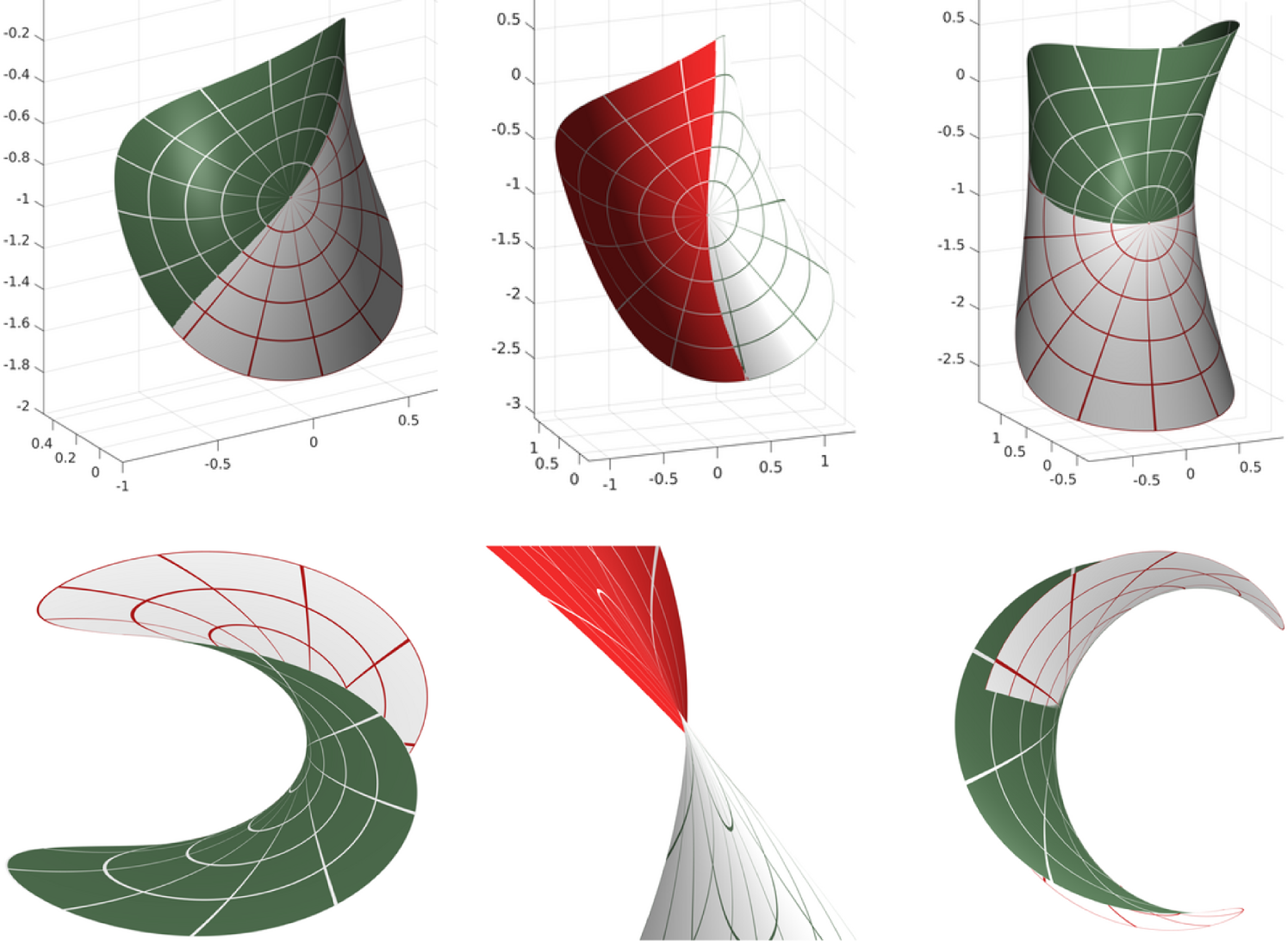
Example 4·8. Local solutions for the potential and initial conditions given above at (4·6) and (4·5) (with
 $\xi_i = 0$
for
 $i\gt-1$
) are computed for the cases:
-
1.
$B= 2-i$
: cuspidal edge at
$z=0$
; -
2.
$B=1-i-i z$
: swallowtail at
$z=0$
; -
3.
$B=2- i z$
: cuspidal cross-cap at
$z=0$
;


and displayed in Figure 4. Note: let Eq denote the equator in
 $\mathbb{S}^2$
perpendicular to the
 $e_3$
-axis, and set
 $C:=N^{-1}(Eq)$
, and
 $C_{cmc} := f_{cmc}(C)$
, i.e.,
 $C_{cmc}$
is the set on
 $f_{cmc}$
corresponding to the singular set on then maximal surface. Then, in the images,
 $C_{cmc}$
is parallel exactly to the
 $e_3$
-axis at the swallowtail singularity, and perpendicular to the
 $e_3$
-axis at the cuspidal cross-cap (see theorem 6·1 below).
4·4. The generic singularities for maximal surfaces
To understand the generic singularities for maximal surfaces, first observe that a non-holomorphic harmonic map N through
 $p \in \mathbb{S}^2$
is precisely given by an initial condition
 $F_0 \in SU(2)$
, plus a normalised potential form:
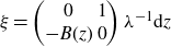 $\xi = \begin{pmatrix} 0 & 1 \\- B(z) & 0\end{pmatrix} \lambda^{-1} \textrm{d} z$
. The map N is obtained as
 $N= \mathrm{Ad} _F E_3$
, whre
 $E_3 = \mathrm{diag}(i -i)$
and F is the SU(2) frame obtained from the potential
 $\xi$
via the DPW method, integrating with the initial condition
 $\Phi(z_0)=F_0$
. The frame F for N has the freedom of right multiplication by any map in into the diagonal subgroup K, thus we can assume that the initial condition
 $F_0$
is of the form:
 \begin{equation*} F_0 = \begin{pmatrix} r & \sqrt{1-r^2}e^{i c} \\ -\sqrt{1-r^2}e^{-ic} & r \end{pmatrix}, \quad \quad r \in [0,1], \quad c \in \mathbb{R} /2\pi \mathbb{Z}.\end{equation*}
Conversely, given a local harmonic map N, an SU(2) frame can be chosen with an initial condition of the above form, and the normalised potential obtained via the Birkhoff decomposition is unique and, after a change of coordinates, has the form of
 $\xi$
above.
Thus the data for a local solution for a non-holomorphic harmonic map, and hence for a local generalised maximal surface f in
 ${\text{Nil}^{3}_{1}}$
is the triple
 $(r,c, B(z)) \in [0,1] \times \mathbb{R} /2\pi \mathbb{Z} \times \mathcal{O}(0)$
, where
 $\mathcal{O}(0)$
denotes the vector space of germs of holomorphic functions at 0. The value of c has no geometric significance, since changing c amounts to a rotation about the
 $e_3$
axis, an isometry of both
 $\mathbb{S}^2$
and of
 ${\text{Nil}^{3}_{1}}$
. We therefore, without loss of generality, take
 $c=0$
and regard the space of local solutions as being
 $[0,1] \times \mathcal{O}(0)$
. Additionally, N takes values in the unit circle in the
 $e_1e_2$
plane (and hence f is singular) at
 $z=z_0$
if and only if
 $r = 1/\sqrt{2}$
. Setting
 $\delta(z) = B(z)-1$
in theorem 4·4 we obtain:
Theorem 4·9. The set of local generalised maximal surfaces f with
 $f(0)=p$
is in one to one correspondence with the set
 $[0,1] \times \mathcal{O}(z_0)$
. If
 $(r,\delta)$
is the data for a local solution f, then f is singular at
 $z=z_0$
if and only if
 $r=1/\sqrt{2}$
. A singularity at
 $z_0$
is non-degenerate if and only if
 $\delta(z_0) \neq 0$
. A non-degenerate singularity at
 $z_0$
is
 $\mathcal{A}$
-equivalent to a
 $:$
-
(i) cuspidal edge if and only if
$\Re \delta(z_0) \neq 0$
and
$\Im \delta(z_0) \neq 0$
$;$
-
(ii) swallowtail if and only if
$\Re(\delta(z_0)) = 0$
,
$\Im \delta(z_0) \neq 0$
,
$\Im \delta'(z_0) \neq 0$
$;$
-
(iii) cuspidal cross-cap if and only if
$\Im \delta (z_0) = 0$
,
$\Re(\delta(z_0)) \neq 0$
and
$\Im(\delta '(z_0)) \neq 0$
.


Since the local solution f through p obtained from a pair
 $(r,\delta) \in [0,1] \times \mathcal{O}(z_0)$
depends analytically on the pair
 $(r,\delta)$
, it is reasonable to use the codimension in the space
 $[0,1] \times j^k \mathcal{O}(0)$
, (where
 $j^k \mathcal{O}(0)$
denotes the finite dimensional space of k-jets at 0), to define the genericity of the local solution. At the k-jet level, an m-parameter family of local solutions is given by a family:
 $\Phi(s,z)= (r(s),j^k \delta^s(z))$
. For a cuspidal edge singularity, there is, generically, one condition (
 $r(s)=1/\sqrt{2}$
) on
 $\Phi(s,-)$
, and for both the swallowtail and cuspidal cross-cap there is one additional condition. In other words the space of cuspidal edges is a co-dimension 1 submanifold whilst the other two are co-dimension 2 submanifolds. A generic 2-parameter family of solutions intersects these spaces transversely. Therefore, at the surface level, each of these singularity types is generic. Finally, these are the only singularities in a generic family of solutions: a solution at s is singular if and only if
 $r(s) = 1/\sqrt{2}$
. Given this, if both the real and imaginary parts of
 $\delta^s(0)$
are non-zero then the singularity is necessarily a cuspidal edge. Otherwise, we can have one more condition in the generic case, and this is either
 $\Im (\delta^s(0))=0$
, or
 $\Re (\delta^s(0))=0$
, so either a swallowtail or cuspidal cross cap.
5. Singularities via the Cauchy problem
5·1. The Cauchy problem for a harmonic map into
$\mathbb{S}^{2}$

In view of Example 4·8, it seems interesting to compare the behaviour of the harmonic map N along the equator with the type of singularity of the corresponding maximal surface. Such an investigation involves solving the Cauchy problem along a curve, which we could then take to be the equator. Note that it is common to consider Björling type problems (where the surface and its normal are prescribed along a curve) as the Cauchy problem for surfaces in 3-dimensional spaces. In the case that the Gauss map determines the surface, the problem of constructing all solutions is similarly addressed by the Cauchy problem for the Gauss map. However, if we are interested in singularities it is natural to use the Gauss map: for the Cauchy problem for the surface, it is not clear what curve you should take as your initial curve, since there are various types of “singular curve”. On the other hand, the Cauchy problem for the Gauss map along a singular curve is clear: the Gauss map takes values in the equator of the sphere. We therefore describe next how to solve the Cauchy problem for a harmonic map into
 $\mathbb{S}^2$
via the DPW method.
Theorem 5·1. Let J be an interval, and suppose given analytic maps,
 $N_0: J \to \mathbb{S}^2$
and
 $W: J \to \mathbb{S}^2$
, such that
 $\langle W,N_0 \rangle =0$
. Then, on an open set
 $U \subset \mathbb{C}$
containing the real interval
 $J \times \{0 \}$
, there is a unique harmonic map
 $N: U \to \mathbb{S}^2$
satisfying the Cauchy conditions
 $:$
 \begin{equation*} N(x,0)=N_0(x), \quad \quad N_y(x,0) = W(x). \end{equation*}
The solution is produced via the DPW method with potential
 $:$
 \begin{equation*} \xi(z) = \frac{1}{2}\left(((\kappa_1(z)-i) E_1 + \kappa_2(z) E_2)\lambda^{-1} + 2\kappa_3(z) E_3 + (\kappa_1(z) + i) E_1 + \kappa_2(z) E_2) \lambda\right) \textrm{d} z,\end{equation*}
where
 $\kappa_1$
,
 $\kappa_2$
and
 $\kappa_3$
are holomorphic extensions of the functions
 $:$
 \begin{equation} \kappa_1(x) = \langle N_0'(x), W (x) \rangle, \; \kappa_2(x) = \langle N_0'(x), N_0(x) \times W(x) \rangle, \; \kappa_3 = \langle W'(x), N_0(x) \times W(x) \rangle.\end{equation}
Conversely, any harmonic map into
 $\mathbb{S}^2$
can be locally represented this way in terms of Cauchy data along a curve.
Proof. The proof is a modification of the proof of theorem 4·4 of [Reference Brander3], replacing the Cauchy data for a spherical surface with the Cauchy data for its harmonic Gauss map. Since a harmonic map into
 $\mathbb{S}^2$
corresponds exactly to a spherical surface, we only need to demonstrate the formulas for
 $\kappa_i$
above. An extended frame F for the solution has Maurer–Cartan form:
 $F^{-1} \text{d} F = (U_{p}\lambda^{-1} + U_{\mathfrak{k}}) \text{d} z + (-\bar{U}_{\mathfrak{k}}^{t} - \bar{U}_{\mathfrak{p}}^{t} \lambda ) \text{d} \bar{z}$
. The Cauchy problem can be solved by finding the restriction of this to the real line and then extending holomorphically to obtain the DPW potential for the solution. The solution potential is thus a holomorphic extension of:
 \begin{equation*} F_0^{-1} \textrm{d} F_0 = (U_{\mathfrak{p}} \lambda^{-1} + U_{\mathfrak{k}}-\bar U_{\mathfrak{k}}^t -\bar U_{\mathfrak{p}}^t \lambda) \textrm{d} x,\end{equation*}
where
 $F_0$
is the extended frame for the harmonic map along the curve
 $y=0$
. The frame used in [Reference Brander3] satisfies:
 \begin{equation} N= \mathrm{Ad}_F E_3, \quad N_y = -\mathrm{Ad}_F E_2, \quad N \times N_y = \mathrm{Ad}_F E_1,\end{equation}
where
 $E_1$
,
 $E_2$
and
 $E_3$
are an orthonormal basis for
 $\mathfrak{su}(2)$
, chosen such that the Lie bracket is the same as the cross-product. Since N has no branch points, we assume without loss of generality that
 $N_y \neq 0$
. Using
 $N_y = -\mathrm{Ad}_F E_2$
along
 $y=0$
we can write
 \begin{equation*} U_{\mathfrak{p}} = (1/2)((\kappa_1-i)E_1 + \kappa_2 E_2), \quad \quad U_{\mathfrak{k}} = (1/2)(\kappa_3+di) E_3, \end{equation*}
where
 $\kappa_i$
and d are some real-valued functions. Then
 \begin{equation*} W'(x) = N_{yx}(x,0) = -\mathrm{Ad}_F([U-\bar U^t, E_2]), \quad \quad F^{-1}F_z = U-\bar U^t. \end{equation*}
Since
 $U_{\mathfrak{p}}-\bar U_{\mathfrak{p}}^t = \kappa_1 E_1+\kappa_2 E_2$
and
 $U_{\mathfrak{k}}-\bar U_{\mathfrak{k}}^t= \kappa_3 E_3$
, this becomes, using (5·2) along
 $y=0$
,
 \begin{equation*} W'(x) = -\kappa_1 N_0(x)+ \kappa_3 N_0 \times W(x).\end{equation*}
Similarly we obtain, along
 $y=0$
:
 \begin{equation*} N'(x) = \kappa_1 W(x) + \kappa_2 N_0(x) \times W(x).\end{equation*}
These give the claimed formulae for
 $\kappa_1$
,
 $\kappa_2$
and
 $\kappa_3$
.
Remark 5·2. For the purpose of numerical implementations, setting
 $E_1 = \mathrm{off-diag}(-i,-i)/2$
,
 $E_2 = \mathrm{off-diag}(1,-1)/2$
and
 $E_3 = \mathrm{diag}(i,-i)/2$
, the above formula for
 $\xi$
becomes:
 \begin{align} \xi(z) =\frac{1}{4}\begin{pmatrix} 2 \kappa_3 i & \def\lumina\hspace{-1.5cm}(\kappa_2-1-\kappa_1 i)\lambda^{-1} + (\kappa_2 +1-\kappa_1 i)\lambda \\ (-\kappa_2-1-\kappa_1 i)\lambda^{-1} +(1-\kappa_2-\kappa_1 i)\lambda & -2 \kappa_3 i \end{pmatrix} \textrm{d} z.{}_{\vphantom{\big(_{;_{1_{1_{1_{1}}}}}}} \end{align}
From this we see that the regularity condition
 $a(z) \neq 0$
, which ensures that the harmonic map is nowhere holomorphic is:
 \begin{equation} \kappa_2- \kappa_1 i \neq 1. \end{equation}
5·2. The Cauchy problem along the equator
Using theorem 5·1, we can write down a potential for an arbitrary harmonic map
 $N: \mathbb{C} \supset \Omega \to \mathbb{S}^2$
that takes the real line into a great circle. For the case of the horizontal equator, all possible Cauchy data N and W are of the form:
 \begin{equation} N(x) = (\cos(\theta(x)), \sin(\theta(x)),0), \quad W(x) = -\cos(\phi(x)) V(x) + \sin(\phi(x))(0,0,1),\end{equation}
where
 $V(x)=(-\sin(\theta(x)),\cos(\theta(x)),0)$
is the unit tangent to N, and
 $\theta(x)$
,
 $\phi(x)$
are arbitrary real-valued functions such that the speed
 \begin{equation*}v(x):= \theta'(x) \neq 0,\end{equation*}
for all x. The formulas at (5·1) are here:
 \begin{equation} \kappa_1(x) = -v(x) \cos(\phi(x)), \quad \kappa_2 (x) = -v(x) \sin(\phi(x)), \quad \kappa_3 (x) = -\phi'(x).\end{equation}
The regularity condition (5·4) is
 $iv e^{i\phi} \neq 1$
, which becomes:
 \begin{equation*} (v,\phi) \neq \pm (1, -\pi/2).\end{equation*}
If we take the potential (5·3), with these values of
 $\kappa_i$
, and integrate with the identity as the initial condition, we obtain a harmonic map
 $\tilde N$
that maps the real line to a great circle in
 $\mathbb{S}^2$
. Because of the choice of frame (5·2), and the initial condition, we can deduce that the circle is in the plane spanned by
 $\tilde N(0,0) = E_3$
and
 $\tilde N_x(0,0)$
. To obtain a map that maps the real line to the equator in the
 $E_1 E_2$
-plane, we need to choose a different initial condition, namely an element
 $F_0 \in SU(2)$
that rotates rotates this plane to the
 $E_1 E_2$
-plane. Differentiating the formula
 $\tilde N = \mathrm{Ad}_F E_3$
, we have
 \begin{eqnarray*}\tilde N_x (0,0) &= &\mathrm{Ad}_F [U - \bar U^t, E_3] \\&=& [\kappa_1 E_1 + \kappa_2 E_2, E_3 ], \quad\quad \text{at } z=0,\\&=& v(0) ( \cos(\phi(0)) E_2 - \sin(\phi(0)) E_1).\end{eqnarray*}
Solving
 \begin{equation*} \mathrm{Ad}_{R_0} E_3 = E_1, \quad \mathrm{Ad}_{R_0} \tilde N_x(0,0) \propto E_2\end{equation*}
gives the initial condition:
 \begin{equation} R_0 = \frac{1}{\sqrt{2}} \begin{pmatrix} e^{-i\alpha} & \lambda e^{i\alpha}\\ -\lambda^{-1} e^{-i \alpha} & e^{i \alpha} \end{pmatrix}, \quad \alpha=\frac{\phi(0)}{2}.\end{equation}
In summary:
Theorem 5·3. Let v and
 $\phi$
be a pair of real analytic functions from an interval I into
 $\mathbb{R}$
, with
 $v(t)\gt0$
. Let N be the harmonic map in
 $\mathbb{S}^2$
given by the potential
 $\xi$
at (5·3), with
 $\kappa_i$
given by the holomorphic extensions of the functions at (5·6). Then N maps the real line into a great circle. If the potential is integrated with the initial condition (5·7), then this great circle lies in the plane perpendicular to
 $E_3$
.
5·3. Singularity type via the Cauchy problem
As always, the product of 2, the (1,1)- and (2,1)- entries of the initial condition
 $R_0$
in (5·7) with
 $\lambda =1$
(see the sentences before theorem 4·6) gives
 $(i g \omega)(p)$
, so we have
 \begin{equation*} (g\omega)(0) = i e^{-i \phi(0)}.\end{equation*}
To determine the singularity type using corollary 4·7, we first remove the diagonal term in (5·3) by the diagonal gauge
 $D_+ = \mathrm{diag} (\exp(-\int i \kappa_3/2\, \textrm{d} z),\exp(\int i\kappa_3/2\, \textrm{d} z))$
as
 $C_2 = C D_+$
. Then
 $C_2$
satisfies
 $\textrm{d} C_2 = C_2 \xi_2$
as
 \begin{equation*}\xi_2(z) =\begin{pmatrix}0 & a(z) \lambda^{-1} + c(z) \lambda \\b(z)\lambda^{-1} + d(z) \lambda & 0\end{pmatrix} \textrm{d} z,\end{equation*}
where
 \begin{align*}a &= \frac14 \exp\left(i \int_0^z \kappa_3\, \textrm{d} z\right)(\kappa_2-1-\kappa_1 i),\quad c = \frac14 \exp\left(i \int_0^z \kappa_3\, \textrm{d} z\right)(\kappa_2+1-\kappa_1 i), \\ b &= \frac14 \exp\left(-i \int_0^z \kappa_3\, \textrm{d} z\right)(-\kappa_2-1-\kappa_1 i), \quad d = \frac14 \exp\left(-i \int_0^z \kappa_3\, \textrm{d} z\right)(1-\kappa_2-\kappa_1 i).\end{align*}
Scaling the coordinate
 $\int_0^z a(w) \textrm{d} w$
by
 $-i e^{ i \phi (0)}$
in the proof of corollary 4·7, gives the normalisation
 $(g \omega) (0) =1$
, and hence:
Theorem 5·4. Retain the assumptions in theorem 5·3 and take the spacelike maximal surface f in
 ${\text{Nil}^{3}_{1}}$
through the DPW method by the potential
 $\xi$
with the initial condition in (5·7). Then f is singular along the interval
 $I \subset \mathbb R$
containing 0. Consider the conformal change of coordinates
 $\zeta=\zeta(z)$
given by
 $:$
 \begin{equation*}\zeta(z) = i e^{-i\phi(0)}\int_0^z a(w) \textrm{d} w, \end{equation*}
where a(z) is the holomorphic extension of
 $:$
 \begin{equation*} a(x) =\frac14 \left(- v(x)\sin \phi(x) -1+i v(x) \cos \phi(x)\right) \exp(-i (\phi(x)-\phi(0))).\end{equation*}
Then the singularity criteria in theorem 4·4 can be applied to the coefficient function
 $\hat B(\zeta)$
of the Abresch–Rosenberg differential
 $\hat B(\zeta) \textrm{d} \zeta^2$
. As a function of z, we have
 $:$
 \begin{equation} \hat B( \zeta(z)) = \frac{i v(z) -e^{i \phi(z)}}{i v(z) - e^{-i \phi(z)}}. \end{equation}
Note: to obtain the formula (5·8), write
 \begin{equation*} \hat B(\zeta) (\textrm{d} \zeta)^2 = -a(z) b(z) (\textrm{d} z)^2 = \frac{b(z)}{a(z)} e^{2i\phi(0)} (\textrm{d} \zeta)^2, \end{equation*}
and substitute
 \begin{equation*}4a(z) = (\kappa_2(z)-1-\kappa_1(z)i)e^{i \int_0^z \kappa_3 \textrm{d} z}, \quad4 b(z) = (-\kappa_2(z)-1-\kappa_1(z) i) e^{-i \int_0^z \kappa_3 \textrm{d} z},\end{equation*}
using the formulas in terms of v and
 $\phi$
at (5·6).
Remark 5·5. At the point
 $z=\zeta=0$
, the values that determine the singularity type are:
 \begin{equation*}1-\Re(\hat B)\big|_{z=0} =\frac{2 (v + \sin \phi) \sin \phi }{1+2v \sin \phi + v^2},\end{equation*}
 \begin{equation*} \Im(\hat B)\big|_{z=0} = \frac{2 \sin \phi \cos \phi} {1+ 2v \sin \phi + v^2}.\end{equation*}
According to theorem 4·4, we have a cuspidal edge at
 $z=0$
provided:
 \begin{equation} 0 \neq \phi(0) \neq \pm \pi/2 \quad \text{and} \quad v(0) \neq -\sin (\phi(0)).\end{equation}
Consider now the criteria of theorem 4·4 for cuspidal cross-cap and swallowtail singularities. The condition
 $\Im(\hat B)' \neq 0$
, needed for both singularities, will hold generally provided
 $\phi'(0) \neq 0$
. Assuming this, arbitrary choices of v and
 $\phi$
that make the first expression above vanish but not the second, i.e.:
 \begin{equation} v(0)=- \sin (\phi(0)), \quad \quad 0 \neq \phi(0) \neq \pm \pi/2\end{equation}
will have a swallowtail singularity at
 $z=0$
. Likewise, choices that make the second expression vanish but not the first, i.e.:
 \begin{equation} \phi(0) = \pm \pi/2, \quad \quad v(0) \neq -\sin (\phi(0)),\end{equation}
will result in a cuspidal cross-cap singularity.
From (5·5),
 $\phi(0)$
is the angle between
 $N_y$
and the
 $E_1 E_2$
-plane. Thus, geometrically, the behaviour of the Gauss map at a cuspidal cross-cap is clear: if coordinates are chosen so that
 $N_x$
is parallel to the equator, then the cuspidal cross-cap occurs generically if
 $N_y(0)$
is parallel to the
 $E_3$
axis. On the other hand, for a swallowtail, the angle between
 $N_y(0)$
and the
 $E_1 E_2$
-plane must be a specific value depending on the ratio
 $v(0)/1$
of the speed of
 $N_x$
to the (unit) speed of
 $N_y$
, namely
 $\phi(0) = \arcsin(-v(0))$
.
Example 5·6. A local solution for a swallowtail, taking
 $v(x)=-1/\sqrt{2}$
and
 $\phi(x) = x+\pi/4$
, and for a cuspidal cross-cap, taking
 $v(x)=1$
and
 $\phi(x)=x + \pi/2$
are computed and shown in Figure 5. Left to right are shown the Gauss map, the maximal surface in
 ${\text{Nil}^{3}_{1}}$
, and the CMC surface in
 $\mathbb{R}^3$
with the same Gauss map.
Solutions to the geometric Cauchy problem using theorem 5·4. See Example 5·6. Top: swallowtail. Bottom: cuspidal cross-cap.

6. Geometry of the associated CMC surface and an application
6·1. The equatorial curve on the CMC surface
Let
 $N: \mathbb{D} \to \mathbb{S}^2$
be a nowhere holomorphic harmonic map, fix an embedding of
 $\mathbb{S}^2$
into
 $\mathbb{R}^3= \mathfrak{su}(2)$
, and let f and
 $f_{cmc}$
denote the associated maximal suface in
 ${\text{Nil}^{3}_{1}}$
, and CMC
 $1/2$
surface in
 $\mathbb{R}^3$
respectively (see theorem 3·4). As in Example 4·8, let
 $C_{cmc}$
denote the set
 $f_{cmc}(C)$
where
 $C \subset \mathbb{D}$
is the preimage under N of the equator in the
 $E_1 E_2$
-plane, which we may call the equatorial curve in the image of
 $f_{cmc}$
. It is the set of points on the CMC surface where the surface normal is perpendicular to
 $E_3$
. The map
 $f_{cmc}$
is regular, hence
 $C_{cmc}$
is a regular curve in
 $\mathbb{R}^3$
.
Theorem 6·1. Let N, f and
 $f_{cmc}$
be above, and let p be a non-degenerate singular point. The maximal surface f has a cuspidal cross-cap singularity at p if and only if the tangent at
 $f_{cmc}(p)$
to the equatorial curve is perpendicular to
 $E_3$
, and a swallowtail at p if and only if the tangent is parallel to
 $E_3$
.
Proof. This follows from the equations (1·1) relating a CMC surface to its harmonic Gauss map. We can always locally choose coordinates as in theorem 5·3, with
 $z=0$
corresponding to p. Then the condition (CC), namely
 $\phi(0)= \pm \pi/2$
and
 $v(0) \neq -\sin(\phi(0))$
is equivalent to f having a cuspidal cross-cap singularity. In the notation of section 1·2, we have
 $f_{cmc}= f^-$
, and from (1·1) this satisfies the equations:
 \begin{equation*} f^-_x = N \times N_y \, -N_x, \quad \quad f^-_y = -N \times N_x \, -N_y.\end{equation*}
Since
 $\phi(0)=\pm \pi/2$
, we have
 $N_x \perp N_y$
at
 $z=0$
, hence:
 \begin{equation*} f^-_x(0) \parallel N_x(0), \quad \text{and} \quad f^-_y(0) \parallel N_y(0).\end{equation*}
Since
 $\gamma(x)= f^-(x,0)$
is locally the equatorial curve, the tangent
 $f^-_x(0)$
to the curve at p is parallel to
 $N_x(0)$
, which is perpendicular to
 $E_3$
. Conversely, if the tangent is perpendicular to
 $E_3$
then, by the same equations,
 $N_y$
must be perpendicular to
 $N_x$
, so
 $\phi(0)=\pm \pi/2$
. The other condition,
 $v(0) \neq -\sin(\phi(0))$
, holds because we assumed that the singular set is non-degenerate.
For the swallowtail condition, again using the setup (5·5) of theorem 5·3, we have:
 \begin{equation*} N_x(0) = v(0)V(0), \quad \quad N_y(0) = -\cos(\phi(0)) V(0) + \sin (\phi(0)) E_3, \end{equation*}
and
 $N(0) \times V(0) = E_3$
. This give:
 \begin{eqnarray*} f^-_y(0) &=& - N \times N_x - N_y \\ &=& -(v(0)+\sin(\phi(0))) E_3 + \cos (\phi(0)) V(0), \end{eqnarray*}
so
 $v(0) = -\sin(\phi(0))$
if and only if
 $f^-_y(0)$
is parallel to V(0), or equivalently, since
 $f^-$
is conformally immersed,
 $f^-_x(0)$
is parallel to
 $f_y \times N$
, i.e. parallel to
 $V(0) \times N(0) = E_3$
. For the converse direction, if the equatorial curve is parallel to
 $E_3$
, the second condition for the swallowtail,
 $0 \neq \phi(0) \neq \pm \pi/2$
, holds because
 $f^-$
is regular, so
 $f^-_y$
above cannot be zero.
6·2. Spacelike maximal discs with natural boundary
As shown in section 3·2, there are no complete spacelike maximal surfaces in
 ${\text{Nil}^{3}_{1}}$
. The simplest “global” regular surface one can contemplate can be defined as follows:
Definition 6·2. Let
 $\mathbb{S}^2_+ := \{ x \in \mathbb{S}^2 ~|~ x_3 \gt 0\}$
, and denote its closure by
 $\overline{\mathbb{ S}^2_+}$
. Let
 $\mathbb{D}$
be a contractible domain in
 $\mathbb{C}$
and
 $N: \mathbb{D} \to \mathbb{S}^2$
be a nowhere holomorphic harmonic map, with the property that N maps a closed set contained in
 $\mathbb{D}$
diffeomorphically to
 $\overline{\mathbb{S}^2_+}$
. Denote by
 $\Omega$
the open subset
 $N^{-1}(\mathbb{S}^2_+)$
. Then the corresponding generalised maximal surface
 $f: \Omega \cup \partial \Omega \to {\text{Nil}^{3}_{1}}$
is called a (spacelike) maximal disc with null boundary.
Note that the restriction
 $f|_\Omega: \Omega \to {\text{Nil}^{3}_{1}}$
is a regular maximal surface, which extends to a generalised maximal surface
 $f: \mathbb{D} \to {\text{Nil}^{3}_{1}}$
, and that the boundary
 $\partial \Omega$
is contained in the singular set of f.
Example 6·3. We can construct examples of a maximal disc with null boundary by taking the DPW potential for a CMC sphere, of the form
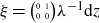 $\xi = {\tiny{\begin{pmatrix} 0 & 1 \\ 0 & 0 \end{pmatrix}}} \lambda^{-1} \textrm{d} z$
and deforming it slightly:
 \begin{equation*} \xi(z) = \begin{pmatrix} 0 & 1 \\ -\epsilon(z) & 0 \end{pmatrix} \lambda^{-1} \textrm{d} z, \end{equation*}
where
 $\epsilon(z)$
is some small holomorphic function, for instance a small constant. An example with
 $\epsilon(z) = 0.04$
is computed and shown in Figure 6.
Example 6·3. Left: Gauss Map. Middle: Maximal surface. Right: CMC surface.

The example shown in Figure 6 has four cuspidal cross-cap singularities on the singular curve. These correspond to the four points on the equatorial curve of the corresponding CMC surface (right) where the tangent is horizontal, as described in theorem 6·1. This illustrates a general principle:
Theorem 6·4. Let
 $f: \Omega \cup \partial \Omega \to {\text{Nil}^{3}_{1}}$
be a spacelike maximal disc with null boundary. Suppose that the boundary singular curve is non-degenerate. Then the boundary curve has at least two cuspidal cross-cap singularities.
Proof. The corresponding CMC surface in
 $\mathbb{R}^3$
is regular, since we assumed the harmonic Gauss map is nowhere holomorphic. The non-degeneracy assumption implies that the boundary curve
 $C= \partial \Omega$
is a regular curve in the open set
 $\mathbb{D}$
containing
 $\Omega \cup \partial \Omega$
. Since C is the inverse image under the Gauss map N of the equator, it is a closed curve, and hence
 $f_{cmc}(C)$
is a regular closed curve in
 $\mathbb{R}^3$
. The third component function of the curve
 $\gamma: C \to \mathbb{R}^3$
given by
 $f_{cmc}|_C$
must have at least one local maximum and at least one local minimum. At these points the tangent is parallel to the
 $E_1E_2$
-plane. Hence the claim follows from theorem 6·1.
Remark 6·5. Theorem 6·4 rules out the existence of a spacelike maximal disc with a cuspidal edge as boundary. Note that for the case where the CMC surface is a sphere the equatorial curve is everywhere parallel to the
 $E_1 E_2$
-plane. In this case the singular curve is everywhere degenerate (since
 $B(z)=0$
). The corresponding maximal surface is a flat disc with a fold singularity at the boundary.