





1. Introduction
An increasing fraction of basic research on turbulent thermal convection is being drawn in recent years from direct numerical simulations (DNS). With this development, it has also become clearer that more attention needs to be paid to numerical convergence, resolution, transient time to steady state, etc. In this paper we attempt to understand transient times needed to achieve the steady state of convection in one dimension, two dimensions, three dimensions and four dimensions, and infer the advantages (or lack thereof) of studying convection in these different dimensions.
Pandey & Sreenivasan (Reference Pandey and Sreenivasan2025) – PS henceforth – obtained transient times from the DNS of two-dimensional (2-D) Rayleigh–Bénard convection (RBC) in a box of aspect ratio
 $\varGamma = 1$
, and Prandtl numbers
 $ \textit{Pr}$
= 0.1 and 1 and for Rayleigh numbers
 $ \textit{Ra}$
between
 $10^6$
and
 $10^{12}$
. (We define
 $ \textit{Ra}$
,
 $ \textit{Pr}$
and
 $\varGamma$
in § 2.) A main conclusion was that long transients with large-scale fluctuating heat transport accompany 2-D convection, which made observations of the ultimate state (Kraichnan Reference Kraichnan1962) quite uncertain. By the ultimate state, we refer to the asymptotic high-
 $ \textit{Ra}$
regime where the Nusselt number scaling surpasses the classical
 $1/3$
exponent and approaches a power of
 $1/2$
(with possible logarithmic corrections).
As another variant of the practically important problem of 3-D convection, one may consider the case of four dimensions, for which the flow occurs in four spatial dimensions and time. There is no instance in the universe for which this configuration applies, yet there are good reasons to consider it. For instance, the Ising universality class has its upper critical dimension equal to 4. That is, for dimension
 $D \geqslant 4$
the renormalisation fixed point controlling the transition is Gaussian, so the leading critical exponents assume mean-field values, possibly with logarithmic corrections. It has been a long-held speculation that turbulence in four dimensions may also have normal scaling with no anomalies. For instance, will the 4-D convection adopt to the ultimate state at a manageably smaller Rayleigh number than in three dimensions?
To obtain a more complete perspective, we also consider heat transport in the 1-D setting. A moment’s thought shows that, when the bottom of a 1-D convection system is heated and its top cooled, heat can be conveyed up only by conduction; there can never be any convection at any
 $ \textit{Ra}$
or
 $ \textit{Pr}$
. (One may interpret this result to mean that the transient state to convection is infinitely long.) In compressible cases, pressure perturbations can travel up and down but, again, there can be no convection. The oscillatory character of pressure has a dependence on
 $ \textit{Pr}$
but the basic result is the same. We present the results only briefly in the body of the text and relegate details to the Supplementary Material (SM).
This paper is thus a study of the influence of dimensionality on thermal convection. Section 2 gives a brief discussion of the simulation parameters, while § 3 discusses the main results. It concludes with a few summary remarks and outlook in § 4. To be concise, we consistently refer to RBC in horizontally periodic boxes as RBC-P. The numerical code Dhara used to compute RBC-P is described and validated in the SM.
2. Simulation details
We perform DNS in 2-D, 3-D and 4-D settings assuming the Oberbeck–Boussinesq model
 \begin{eqnarray} \boldsymbol{\nabla }\boldsymbol{\cdot }{\boldsymbol u} & = & 0, \\[-28pt] \nonumber \end{eqnarray}
 \begin{eqnarray} \frac {\partial {\boldsymbol u}}{\partial t} + {\boldsymbol u} \boldsymbol{\cdot }\boldsymbol{\nabla }{\boldsymbol u} & = & - \frac { \boldsymbol{\nabla }\!p}{\rho _0} + \alpha g (T-T_0) \hat {z} + \nu {\nabla} ^2 {\boldsymbol u}, \\[-28pt] \nonumber \end{eqnarray}
 \begin{eqnarray} \frac {\partial T}{\partial t} + {\boldsymbol u} \boldsymbol{\cdot }\boldsymbol{\nabla }T & = & \kappa {\nabla} ^2 T, \\[-6pt] \nonumber \end{eqnarray}
where
 ${\boldsymbol u}({\boldsymbol r})$
,
 $p({\boldsymbol r})$
and
 $T({\boldsymbol r})$
are, respectively, velocity, pressure and temperature. The space dimensionality of the system is to be treated as appropriate. The acceleration due to gravity is
 $-g \hat {z}$
;
 $\rho _0$
is the reference density,
 $T_0$
is the reference temperature and
 $\alpha , \nu , \kappa$
are the isobaric thermal expansion coefficient, kinematic viscosity and thermal diffusivity, respectively. The dynamics of RBC is governed by
 $ \textit{Ra} = \alpha g \Delta T H^3 / (\nu \kappa )$
and
 $ \textit{Pr} = \nu / \kappa$
, where
 $\Delta T$
is the applied temperature difference between the bottom and top surfaces of the fluid layer of depth
 $H$
. The flow velocities are measured in units of the free-fall velocity
 $u_{\kern-1pt f} = \sqrt {\alpha g \Delta T H}$
and time scale in units of free-fall time
 $t_{\kern-1pt f} = H/u_{\kern-1pt f}$
.
2.1. Direct numerical simulations of 2-D convection
In 2-D convection, the flow is constrained to a vertical plane, with
 ${\boldsymbol u}({\boldsymbol r}) = (u_x, u_z)$
with
 ${\boldsymbol r} = (x, z)$
. We first study the case of a no-slip condition at all walls, the horizontal walls being isothermal and the vertical walls adiabatic. In PS, we have already explored the characteristics of transients for
 $ \textit{Pr} = 0.1$
and
 $ \textit{Pr} = 1$
and for
 $10^6 \leqslant Ra \leqslant 10^{12}$
. Here, we include
 $ \textit{Pr}$
of
 $0.05$
and
 $0.021$
. Direct numerical simulations of 2-D RBC, governed by (2.1)–(2.3), are conducted using a spectral element solver Nek5000 (Fischer Reference Fischer1997). The square domain is decomposed into
 $N_e$
elements, further discretised using Nth-order Legendre polynomials. Details of DNS for
 $ \textit{Pr} = 0.1$
and
 $ \textit{Pr} = 1$
can be found in PS, and those for
 $ \textit{Pr} = 0.021$
in Pandey (Reference Pandey2021). Additional details for
 $ \textit{Pr} = 0.021$
and
 $ \textit{Pr} = 0.05$
are provided in table 1.
Important DNS parameters of RBC in a 2-D box of
 $\varGamma = 1$
:
 $N_e N^2$
is the total number of mesh cells;
 $t_{\textit{sim}}$
is the total duration of simulation in the nominally steady state;
 $ \textit{Nu}$
and
 $\textit {Re}$
are, respectively, the global heat and momentum transports in this state; the error bars are the corresponding standard deviations.

Table 1. Long description
The table presents data on 2-D convection in a square domain, focusing on parameters such as Prandtl number (Pr), Rayleigh number (Ra), number of elements squared (N_e^2), Nusselt number (Nu), Reynolds number (Re), and the simulation time in the nominally steady state (t_sim (tf)). The table has 16 rows and 6 columns. Column headers are Pr, Ra, N_e^2, Nu, Re, and t_sim (tf). Row labels are not explicitly mentioned but are differentiated by their values. Each row provides specific values for each parameter, showing variations across different conditions. Notable trends include increasing Nu and Re with increasing Ra, and varying t_sim (tf) values across different Pr and Ra combinations.
To make direct comparisons with
 $D=3$
and
 $D=4$
, we have performed simulations of 2-D convection also for
 $\varGamma = 1$
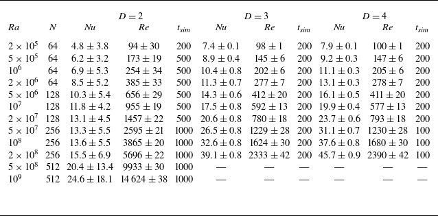
, with periodic sidewalls (RBC-P). These simulations are conducted using the incompressible module of the finite-difference code Dhara (see SM). The gross flow response quantities are summarised in table 2.
Response quantities for RBC-P in
 $D=2, 3$
and
 $4$
,
 $ \textit{Pr}=1$
.
 $N$
is the number of grid points for each spatial dimension (accounting for a total of
 $N^D$
points) used by the finite-difference solver Dhara. Here,
 $ \textit{Nu}$
and
 $\textit {Re}$
values are time averaged, with
 $\pm$
one standard deviation;
 $t_{\textit{sim}}$
is the integration time in units of
 $t_{\kern-1pt f}$
.

Table 2. Long description
The table presents response quantities for RBC-P in various conditions. It has 10 rows and 12 columns. The columns are labeled with different parameters: Ra, N, Nu, Re, t_sim for D = 2, Nu, Re, t_sim for D = 3, and Nu, Re, t_sim for D = 4. The rows list values for these parameters. For example, Row 1: Ra, 2 times 10 to the power of 5; N, 64; Nu, 4.8 plus or minus 3.8; Re, 94 plus or minus 30; t_sim, 200; Nu, 7.4 plus or minus 0.1; Re, 98 plus or minus 1; t_sim, 200; Nu, 7.9 plus or minus 0.1; Re, 100 plus or minus 1; t_sim, 200.
2.2. Direct numerical simulations of 3-D convection
We consider the following configurations with no-slip and isothermal top and bottom walls: (a) closed cube with no-slip condition at all the walls; (b) closed rectangular cuboid of length
 $2.4H$
and width
 $0.8H$
(Pandey et al. Reference Pandey, Schumacher, Parsani and Sreenivasan2026), especially to understand the effects of geometry; and (c) cube with periodic sidewalls (RBC-P). The sidewalls in (a) and (b) are adiabatic. The DNS of RBC are performed for
 $ \textit{Pr} = 0.1, 1, 10$
for
 $ \textit{Ra}$
between
 $10^6$
and
 $10^{10}$
. The higher-
 $ \textit{Ra}$
simulations are carried out on coarser meshes than demanded for a faithful replication of the entire flow structure, but the conclusions on transients do not depend on the resolution, up to a point. In the SM, we examine the consequences of using coarser resolutions on transients; see also PS. The RBC-P cases for
 $ \textit{Pr} = 1$
are conducted using the incompressible module of the finite-difference code Dhara, as summarised in table 2.
2.3. Direct numerical simulations of 4-D convection
Four-dimensional convection is performed in a periodic hypercube of size
 $L_w = L_x = L_y = H$
for
 $ \textit{Pr} = 1$
and Rayleigh numbers between
 $ \textit{Ra} = 10^5$
and
 $2 \times 10^8$
. To ensure a direct comparison, 2-D and 3-D simulations are conducted using a consistent numerical framework, as summarised in table 2. These cases utilise the incompressible module of the finite-difference solver Dhara, which employs a second-order spatial discretisation on a staggered marker-and-cell grid and a third-order Runge–Kutta scheme for time integration.
The computational complexity of 4-D simulations increases strongly with
 $ \textit{Ra}$
. Even for
 $ \textit{Ra} = 2 \times 10^8$
, which was resolved on a
 $256^4$
grid, it represented approximately 4.3 billion degrees of freedom per variable. This specific run was executed on 128 NVIDIA A100 GPUs across 32 compute nodes on the Polaris supercomputer at the Argonne Leadership Computing Facility (ALCF). This simulation required approximately 18 wall-clock hours to reach an integration time of
 $t_{\textit{sim}} = 100$
.
3. Results
3.1. Basic response quantities
The instantaneous state of convection is given by the domain-averaged kinetic energy
 \begin{align} E = \langle \vert {\boldsymbol u} \vert ^2 /2 \rangle _V / u_{\kern-1pt f}^2 . \end{align}
Here, we have
 $E = 0$
in the purely diffusive state of no motion, and
 $E \gt 0$
represents a perturbed state. Temporal evolution of the flow can be described by the evolution of
 $E$
. Once convection is established and the system is in a statistically steady state, the flow strength is measured by the Reynolds number
 $\textit {Re}$
, which is commonly defined in DNS studies using the root-mean-square (r.m.s.) velocity
 \begin{align} \textit {Re} = u_{\textit{rms}} H / \nu , \quad \mbox{where} \quad u_{\textit{rms}} = \sqrt { \langle \vert {\boldsymbol u} \vert ^2 \rangle _{V,t} } . \end{align}
Here,
 $\langle \boldsymbol{\cdot }\rangle _{V,t}$
is the average over the entire domain, and also time in the statistically steady state. The mean kinetic energy in this state is defined as
 $E_{av} = 0.5 u_{\textit{rms}}^2 / u_{\kern-1pt f}^2$
.
The heat transport through the convective layer is quantified using the Nusselt number
 \begin{align} Nu = 1 + \frac {H}{\kappa \Delta T} \langle u_z T \rangle _{V,t} . \end{align}
The globally averaged kinetic energy and thermal dissipation rates can also be used to define Nusselt numbers; their closeness to
 $ \textit{Nu}$
from (3.3) is thought to ensure the spatial and temporal convergence (see Stevens et al. Reference Stevens, Verzicco and Lohse2010 and PS). We have verified that the Nusselt numbers computed using different methods agree within a few per cent.
3.2. One-dimensional flow
Conduction is the only means of transport between top and bottom walls in the incompressible case. While the continuity equation,
 $\partial (\rho u_z) / \partial z = -\partial \rho / \partial t$
(where
 $\rho$
is the density of the fluid), allows for local density variations in the compressible case, the strictly 1-D geometry and impenetrable boundaries at the top and bottom prevent vertical mass flux or bodily overturning – hence no convection. A linear instability analysis and the DNS (both detailed in the SM) confirm this constraint. The determinant of the linearised system is strictly non-zero for all real wavenumbers, mathematically precluding the stationary bifurcation required for classical convection. The system does support oscillatory acoustic modes as
 $ \textit{Ra}$
increases, but these purely longitudinal compressions do not lead to heat transport with a unidirectional motion. (Professor J. Wettlaufer has suggested a possible connection of the present 1-D considerations to highly confined quasi-1-D superfluid systems: there will be no convection in such systems either, but its detailed discussion here takes us too far from the theme of the paper.)
3.3. Two-dimensional convection
We showed in PS, for
 $10^7 \leqslant Ra \leqslant 10^{12}$
, that the scaling of the transient time varies in the range
 $ \textit{Ra}^{0.6}$
to
 $ \textit{Ra}^{0.7}$
, consistent with Lindborg’s theory (Lindborg Reference Lindborg2025), but the coefficient of proportionality depended on
 $ \textit{Pr}$
. We note that Lindborg’s theoretical lower bound corresponds to the global diffusion time
 $H^2/\nu$
, and the transient times observed in our simulations actually exceed this time scale. Recall that the r.m.s. velocity of turbulent convective flows in a 2-D domain does not scale as the free-fall velocity; it is a function of
 $ \textit{Ra}$
and
 $ \textit{Pr}$
. In addition, PS found that
 $u_{\textit{rms}} / u_{\kern-1pt f}$
scales as
 $ \textit{Ra}^{1/6} Pr^{-1/2}$
in the high-
 $\textit {Re}$
regime. This scaling suggests that, in 2-D RBC, it takes longer with increasing
 $ \textit{Ra}$
or decreasing
 $ \textit{Pr}$
to achieve the nominally steady state. This is demonstrated in figure 1, where temporal evolutions of
 $E$
in a 2-D square box are shown for various
 $ \textit{Ra}$
, and
 $ \textit{Pr} = 0.021$
. Figure 1(b) shows that
 $E$
in the initial phase grows exponentially when the convective motion is getting established. However, as seen better in figure 1(a), this initial exponential is followed by another slow exponential growth in the convection state. Only after this extended second growth state does
 $E$
begin to attain a nominal mean that increases with
 $ \textit{Ra}$
, with huge fluctuations around it.
(a) Evolution of
 $E$
for different Rayleigh numbers at
 $ \textit{Pr} = 0.021$
in a closed 2-D square box. Time required to achieve a nominally steady state increases with
 $ \textit{Ra}$
. (b) Energy growth is exponential during the initial phase when the perturbations grow and convective motion is being established. (There are of the order of 100 data points in the initial exponential part.)

Figure 1. Long description
Panel A: A line graph shows the evolution of energy (E) over time (t) for different Rayleigh numbers (Ra) in a closed 2-D square box. The x-axis represents time (t) in units of t_f, ranging from 0 to 4000. The y-axis represents energy (E), ranging from 0 to 2.0. The graph includes multiple lines representing different Rayleigh numbers: Ra = 10^7, Ra = 3 x 10^7, Ra = 10^8, Ra = 4 x 10^8, and Ra = 10^9. The lines show that the time required to achieve a nominally steady state increases with Ra. Panel B: Another line graph shows the initial phase of energy growth, which is exponential. The x-axis represents time (t) in units of t_f, ranging from 0 to 15. The y-axis represents energy (E) on a logarithmic scale, ranging from 10^−11 to 10^−1. The graph includes multiple lines representing different Rayleigh numbers, similar to Panel A. The lines indicate that energy growth is exponential during the initial phase when perturbations grow and convective motion is being established.
For a simulation performed ab initio from the conduction state,
 $E$
evolves in the slow exponential state of convection according to
 \begin{align} [E_{av} - E(t)]/E_{av} = c \exp (-kt) , \end{align}
where
 $c$
is the scaling factor and
 $k$
is the growth rate (see PS). The transient time
 $t_{\textit{trns}}$
is defined as the time that is required for the flow to reach a state, where
 $E$
is a certain fraction of
 $E_{av}$
. Taking, for example,
 $E = 0.96 E_{av}$
in (3.4), the transient time is computed as
 \begin{align} t_{\textit{trns}} = \frac {1}{k} \log \frac {c}{0.04}. \end{align}
Transient times
 $t_{\textit{trns}}$
estimated using (3.5), plotted against
 $ \textit{Ra}$
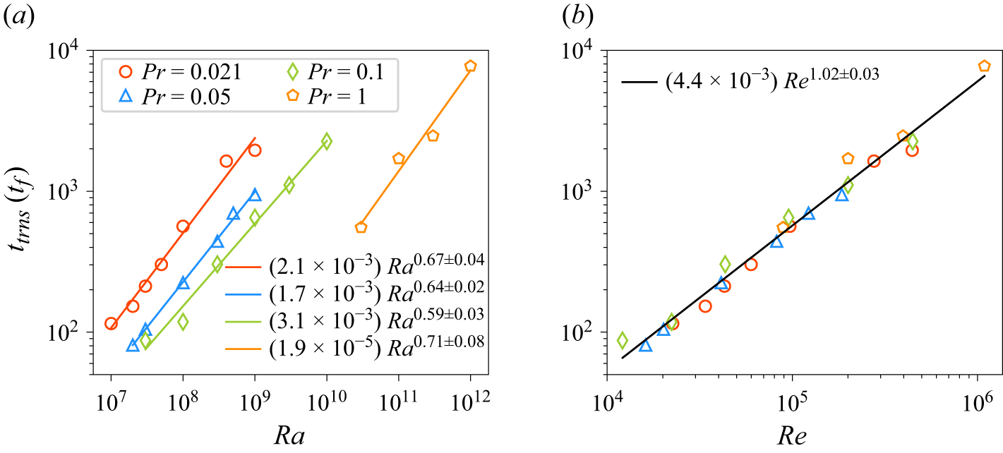
in figure 2(a), show an increase with
 $ \textit{Ra}$
. The best fit exponents vary between 0.59 and 0.71 depending on
 $ \textit{Pr}$
. Consistent with the trend found in PS, they become longer with decreasing
 $ \textit{Pr}$
for a fixed thermal forcing. Figure 2(b) shows
 $t_{\textit{trns}}$
as a function of the flow Reynolds number; data for different Prandtl numbers nearly collapse and the best fits are approximately linear in
 $\textit {Re}$
. The best fit for data at all
 $ \textit{Pr}$
yields
 $t_{\textit{trns}} = 0.0044 \textit {Re}^{1.02}$
.
Transient time
 $t_{\textit{trns}}$
for RBC in a 2-D square box as a function of (a) Rayleigh number and (b) Reynolds number. Solid lines represent best fits. Scaling exponents in (a) depend on
 $ \textit{Pr}$
. Solid black line in (b) is the best fit using data for all
 $ \textit{Pr}$
. Data for
 $ \textit{Pr} = 1$
and
 $ \textit{Pr} = 0.1$
are taken from PS.

It should be stressed that these data are applicable for ab initio calculations (i.e. convection begun from slightly perturbed conduction states). As the steady state kinetic energy is higher for higher
 $ \textit{Ra}$
, there will be a transient period also when the simulation is begun from the lower
 $ \textit{Ra}$
. However, those transient times will be shorter than for the ab initio simulations. The observed linear dependence of the transient time on
 $\textit {Re}$
imposes severe restrictions on the exploration of 2-D convection at high
 $\textit {Re}$
– as could, in fact, be inferred already from Lindborg (Reference Lindborg2025).
3.4. Three-dimensional convection
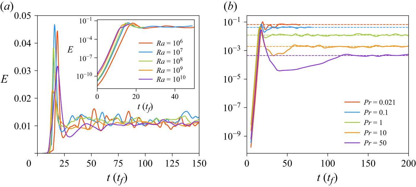
This is the practically relevant case. In figure 3(a), the evolutions of
 $E$
for RBC in a closed cubic domain for
 $ \textit{Pr} = 1$
and
 $10^6 \leqslant Ra \leqslant 10^{10}$
are shown, where the simulations begin from the diffusive state. We observe that
 $E$
grows rapidly in the beginning and starts to fluctuate, achieving a plausible
 $E_{av}$
beyond
 $50$
to
 $70 \, t_{\kern-1pt f}$
. The inset of figure 3(a), where
 $E$
is shown on a logarithmic scale, reveals that the initial growth is exponential as in two dimensions, when the convective motion is getting established. Qualitatively similar evolutions of
 $E$
occur for flows at
 $ \textit{Pr} = 0.1$
and
 $ \textit{Pr} = 10$
. The same is true also for flows in a rectangular cuboid of dimensions
 $L_x = 2.4H$
and
 $L_y = 0.8H$
(Pandey et al. Reference Pandey, Schumacher, Parsani and Sreenivasan2026) – see the SM. Note that, unlike in two dimensions, the variation of
 $E_{av}$
with
 $ \textit{Ra}$
is weaker for
 $ \textit{Pr} \approx 1$
, although
 $E_{av}$
decreases slightly with
 $ \textit{Ra}$
for low-
 $ \textit{Pr}$
fluids, while it increases slightly for high-
 $ \textit{Pr}$
fluids. This is also inferred from the scaling of the Reynolds number in 3-D convection:
 $\textit {Re} \sim Ra^{1/2}$
for
 $ \textit{Pr} \sim 1$
(Chillà & Schumacher Reference Chillà and Schumacher2012; Pandey et al. Reference Pandey, Schumacher, Parsani and Sreenivasan2026),
 $\textit {Re} \sim Ra^{0.44}$
for
 $ \textit{Pr} \lesssim 0.03$
(Pandey & Verma Reference Pandey and Verma2016; Scheel & Schumacher Reference Scheel and Schumacher2017) and
 $\textit {Re} \sim Ra^{0.6}$
for
 $ \textit{Pr} \gg 1$
(Silano et al. Reference Silano, Sreenivasan and Verzicco2010; Horn et al. Reference Horn, Shishkina and Wagner2013; Pandey et al. Reference Pandey, Verma and Mishra2014).
Temporal evolution of
 $E$
for RBC in a closed cubic domain (a) for various
 $ \textit{Ra}$
at
 $ \textit{Pr} = 1$
, and (b) for different flows at
 $ \textit{Ra} = 10^7$
. Inset in (a) reveals that the growth in the initial phase during the setting up of the convective motion is exponential in nature. Dashed horizontal lines in (b) indicate
 $E_{av}$
.

Evolution of
 $E$
for different
 $ \textit{Pr}$
and
 $ \textit{Ra} = 10^7$
in the same cubic domain is shown in figure 3(b). Note that
 $E_{av}$
, and thus
 $\textit {Re}$
, decreases with increasing
 $ \textit{Pr}$
(Pandey & Sreenivasan Reference Pandey and Sreenivasan2021). The logarithmic scale for
 $E$
in figure 3(b) highlights the exponential growth in the beginning, and also a strong dependence of
 $E_{av}$
on
 $ \textit{Pr}$
. The steady state takes slightly longer with increasing
 $ \textit{Pr}$
; thus, it seems that the transient time in three dimensions increases, albeit weakly, with decreasing
 $\textit {Re}$
. However, as a whole, the trends with respect to
 $ \textit{Ra}$
or
 $\textit {Re}$
are not strong as in two dimensions (as one might indeed have expected).
3.5. Four-dimensional convection
3.5.1. Motivation
Here, we consider convection in four spatial dimensions and time. Since 4-D convection never appears in the universe, a few sentences are useful to justify the effort. We recall that Wilson & Fisher (Reference Wilson and Fisher1972) considered systems with spatial dimension of
 $4 -\epsilon$
, where
 $\epsilon \ll 1$
. Their insight was that four dimensions is the upper critical dimension for equilibrium phase transitions, and that Landau’s mean-field theory becomes exact for four dimensions and beyond, with deviations from it arising in fewer dimensions. Indeed, they showed that one can treat the deviation perturbatively in
 $\epsilon$
. Nelkin (Reference Nelkin1974, Reference Nelkin1975) proposed that four spatial dimensions might play an analogous role in turbulence theory, and argued that intermittency arises from fluctuations of the local energy dissipation and cascade transfer rates, which would weaken with increasing dimension. If this conjecture is true,
 $D = 4$
would behave like a mean-field limit for turbulence. This has never been proven, despite some suggestion (Gotoh et al. Reference Gotoh, Watanabe, Shiga, Nakano and Suzuki2007; Yamamoto et al. Reference Yamamoto, Shimizu, Inoshita, Nakano and Gotoh2012) that intermittency weakens with increasing dimensions. The last two papers studied homogeneous and isotropic turbulence.
One of the problems in drawing firm conclusions from these studies is that the DNS in higher dimensions becomes more expensive and so the Reynolds numbers of the DNS are smaller. Although, because of this, it was clear from the outset that the Rayleigh numbers achievable would be quite modest in four dimensions, we regarded that some instructive lesson could arise while making comparisons with three dimensions.
3.5.2. Results
The results of 4-D simulations are summarised in table 2 for
 $ \textit{Pr} = 1$
. Due to the high computational cost associated with the
 $N^4$
grid scaling, these runs currently span Rayleigh numbers from
 $10^5$
to
 $2 \times 10^8$
, but are adequate for drawing a preliminary conclusion.
Temporal evolution of the domain-averaged kinetic energy
 $E$
in a 4-D horizontally periodic domain for
 $ \textit{Pr} = 1$
at various Rayleigh numbers. Similar to the 3-D case, the inset reveals an initial phase of exponential growth as the convective motion is established, followed by a statistically steady state where
 $E$
fluctuates around its mean value
 $E_{av}$
.

As shown in figure 4, the temporal evolution of the kinetic energy
 $E$
in four dimensions is similar to that in three dimensions. After a slightly perturbed conduction state, there is an initial exponential growth phase in which the convective motion is established. The system later enters a statistically steady state characterised by fluctuations around the mean value
 $E_{av}$
. The transient time for reaching this steady state in four dimensions is approximately
 $40$
to
 $50 \, t_{\kern-1pt f}$
, which is somewhat smaller than in three dimensions but comparable overall. The transient times show an increasingly weaker trend with
 $\textit {Re}$
as the dimensionality increases beyond 2; the 3-D and 4-D cases are similar in this regard.
Scaling of global response quantities with
 $ \textit{Ra}$
for RBC-P at
 $ \textit{Pr} = 1$
in
 $D=2, 3$
and
 $4$
. (a) Nusselt number (
 $ \textit{Nu}$
) versus
 $ \textit{Ra}$
. Dashed and solid lines represent power-law fits for low- and moderate-
 $ \textit{Ra}$
regimes, respectively. (b) Reynolds number (
 $\textit {Re}$
) versus
 $ \textit{Ra}$
with global power-law fits. Error bars denote the standard deviation of temporal fluctuations.

However, the Nusselt and Reynolds numbers, presented in figure 5, depend on the dimensionality of convection. Figure 5(a) shows that the Nusselt number at a given
 $ \textit{Ra}$
increases with
 $D$
, although the difference is less conspicuous between three and four dimensions than it is between two and three dimensions. For example, in the range
 $ \textit{Ra} \geqslant 5 \times 10^6$
, the scalings for three dimensions (
 $ \textit{Nu} = 0.22 Ra^{0.27}$
) and four dimensions (
 $ \textit{Nu} = 0.21 Ra^{0.28}$
) share closely similar powers and prefactors. By comparison, the scaling in two dimensions follows
 $ \textit{Nu} = 0.063 Ra^{0.29}$
, although characterised by massive temporal fluctuations. The overall enhancement of
 $ \textit{Nu}$
in higher dimensions stems from the increased spatial degrees of freedom, which allow thermal plumes to advect heat with significantly fewer disruptive interactions. For
 $ \textit{Ra} = 2 \times 10^8$
,
 $ \textit{Nu}$
in three dimensions is roughly
 $2.4$
times that in two dimensions, while that in four dimensions it is only 15 % higher than that in three dimensions. Two-dimensional data show a conspicuous break for a decade around
 $ \textit{Ra} = 10^8$
, which is due to the appearance of a strong zonal flow (Goluskin et al. Reference Goluskin, Johnston, Flierl and Spiegel2014) for this range of
 $ \textit{Ra}$
. The flow structures and their evolutions suggest that 2-D convective flows in a horizontally periodic box of
 $\varGamma = 1$
comprise a strong zonal component for all higher-
 $ \textit{Ra}$
cases in the present work. Consequently, the heat transport is lower than that in a closed square box, as reported by Pandey & Sreenivasan (Reference Pandey and Sreenivasan2025).
Figure 5(b) further highlights a striking difference between two dimensions, on the one hand, and three and four dimensions, on the other: the Reynolds number is higher in two dimensions (
 $\textit {Re} = 0.071 Ra^{0.59}$
) compared with the lower (and nearly indistinguishable) scalings of three and four dimensions (
 $\textit {Re} \approx 0.36 Ra^{0.46}$
). Rather than indicating more intense small-scale turbulence, this elevated
 $\textit {Re}$
in two dimensions is a consequence of enstrophy conservation, which prohibits vortex stretching and forces an inverse cascade of kinetic energy. The resulting accumulation of energy in the largest available scales generates a domain-filling large-scale circulation that inflates the r.m.s. velocity. In three and four dimensions, the availability of vortex stretching enables a forward energy cascade to dissipative scales, severely weakening this domain-sized scale and yielding lower Reynolds numbers. Note that the scaling exponent in two dimensions in the horizontally periodic domain is smaller than
 $2/3$
, which was derived by Lindborg (Reference Lindborg2025) and confirmed numerically by Pandey & Sreenivasan (Reference Pandey and Sreenivasan2025). However, we stress that the scaling
 $\textit {Re} \sim Ra^{2/3}$
is realised only at high enough Rayleigh numbers. Pandey & Sreenivasan (Reference Pandey and Sreenivasan2025) observed that the
 $\textit {Re}$
in the closed square domain exhibits a shallower scaling at lower Rayleigh numbers. In fact, their data for
 $ \textit{Ra}$
between
 $10^7$
and
 $10^9$
for
 $ \textit{Pr} = 1$
are consistent with a
 $\textit {Re} \sim Ra^{0.59}$
scaling, very similar to that found here.
These scaling behaviours also provide a context for commenting on convection at extreme thermal forcing. One might have expected that the additional spatial degree of freedom in four dimensions would trigger a transition to a new scaling regime at a comparatively lower
 $ \textit{Ra}$
. However, our results show that the near-classical power law persists in four dimensions up to
 $ \textit{Ra} = 2 \times 10^8$
. The robustness of these scaling exponents in three and four dimensions suggests that spatial dimensionality does not bypass the fundamental, classical mechanisms of heat transport. Consequently, what ultimately happens to the flow at exceptionally high Rayleigh numbers may remain essentially the same, demanding similarly high levels of thermal forcing for all spatial dimensions.
4. Summary remarks and outlook
In this study, we have explored the influence of spatial dimensionality, ranging from 1 to 4, on the dynamics of thermal convection. We find that the transient time required to achieve a statistically steady convective state is fundamentally tied to the geometric constraints of the system. In the degenerate 1-D case, strict constraints prohibit convection physically and mathematically. In two dimensions, the transient times are exceptionally long and scale approximately linearly with the flow Reynolds number, posing a severe computational bottleneck for exploring very high-
 $ \textit{Ra}$
regimes. As the dimensionality increases to three and four dimensions, the dependence of the transient duration on
 $\textit {Re}$
becomes markedly weaker. The temporal evolution of the kinetic energy in four dimensions closely mirrors that of three dimensions, confirming that the transition to a steady state becomes more efficient and less dependent on thermal forcing when sufficient spatial degrees of freedom are available.
Based on our findings on the transient time in systems of dimensions one to four, we construct the following empirical relation:
 \begin{align} \mbox{Transient time} /t_{\kern-1pt f} = \beta \textit {Re}^\eta , \quad \mbox{where} \quad {\eta } = \frac {(D-3)(D-4)}{2(D-1)} . \end{align}
The prefactor
 $\beta \approx 40$
for three and four dimensions, whereas
 $\beta \approx 4.4 \times 10^{-3}$
for two dimensions.
We may now state our conclusions as follows. First, given the long transient times in two dimensions, it appears that a decisive study of the ultimate state of convection in two dimensions requires an unduly long computational time – which, in fact, may never be possible at extremely high Reynolds numbers. Second, for 3-D convection,
 $t_{\textit{trns}}$
is of the order of 50 free-fall times. Third, if it is possible to treat 3-D convection as a perturbation of 4-D convection, there may be some merit to studying 4-D convection to determine various scaling problems, including the ultimate state. However, even if the 4-D case behaves like the mean-field model and the 3-D case can be conceived as a perturbation from four dimensions, we should expect that, at the level of accuracy with which we have been able to determine the transient times, we should not expect in this regard a huge differences between the 3-D and 4-D cases.
Supplementary material
Supplementary material is available at https://doi.org/10.1017/jfm.2026.11981.
Acknowledgements
We thank Shreshthi for providing data of figure 3(b) in the SM, and J. Wettlaufer for comments on a preliminary draft. The authors gratefully acknowledge Dalma and Jubail clusters at NYU Abu Dhabi for providing computational resources. We also thank ALCF for computing time on Polaris via the Director’s Discretionary Program.
Funding
This material is based upon work supported by Tamkeen under the NYU Abu Dhabi Research Institute grant G1502. A.P. also acknowledges financial support from ANRF (formerly SERB), India under the grant SRG/2023/001746. H.T. thanks IIT Kanpur for the Fellowship for Academic and Research Excellence (FARE). NYU supports the research of K.R.S.
Declaration of interests
The authors report no conflict of interest.
Data availability statement
The data that support the findings of this study are available from the corresponding author upon reasonable request.


 Γ=1
 NeN2
 tsim
 Nu
 Re
 D=2,3
 4
 Pr=1
 N
 ND
 Nu
 Re
 ±
 tsim
 tf

 E
 Pr=0.021
 Ra
 ttrns
 Pr
 Pr
 Pr=1
 Pr=0.1
 E
 Ra
 Pr=1
 Ra=107
 Eav

 E
 Pr=1
 E
 Eav

 Ra
 Pr=1
 D=2,3
 4
 Nu
 Ra
 Ra
 Re
 Ra


 Open access

