Implications
Lambing distribution can be viewed as a typical example of circular data distributed on a round-year parametric space. This is a highly relevant trait for most meat-type production systems. The Ripollesa data set has been analyzed under a heteroskedastic circular mixed model and revealed both direct and residual genetic backgrounds for lambing distribution, as well as a positive and high genetic correlation among them; other systematic and environmental sources of variation were also discussed. This study contributes the breeding ground for future genetic selection programs on sheep seasonality and lambing distribution.
Introduction
Unlike most domestic livestock species, sheep are widely known as an animal with a marked seasonality of breeding activity (Rosa and Bryant, Reference Rosa and Bryant2003). Maximum reproductive activity is typically associated with short days, with the highest percentage of ewes displaying estrus and ovulatory activity during the late summer, autumn and early winter (Chemineau et al., Reference Chemineau, Bodin, Migaud, Thiéry and Malpaux2010). The consequent seasonal pattern of sheep meat and milk production inevitably impacts on other variables such as trade, consumption and lamb prices (Chemineau et al., Reference Chemineau, Malpaux, Brillard and Fostier2007). Within this context, the reduction of ewe seasonality could be viewed as an appealing strategy for the sheep industry in most countries with mild seasons. Some seasonality-related traits have been suggested to be heritable in sheep (Quirke et al., Reference Quirke, Hanrhan, Loughnane and Triggs1986; Al-Shorepy and Notter, Reference Al-Shorepy and Notter1997; Notter, Reference Notter2008), although this trait has never been analyzed in depth with proper models.
As reported by Casellas et al. (Reference Casellas, Martín de Hijas-Villalba and Id-Lahoucine2019) in the companion paper, lambing distribution is a real example of circular data distributed around a circular parametric space from 1 January to 31 December. This can be analyzed by circular mixed models (Mulder and Klugkist, Reference Mulder and Klugkist2017; Casellas et al., Reference Casellas, Martín de Hijas-Villalba and Id-Lahoucine2019) using the von Mises distribution (Fisher, Reference Fisher1993). Moreover, this parametrization can even account for heteroskedacity as proposed by SanCristobal-Gaudy et al. (Reference SanCristobal-Gaudy, Elsen, Bodin and Chevalet1998) and Ibáñez-Escriche et al. (Reference Ibáñez-Escriche, Sorensen, Waagepetersen and Blasco2008a and Reference Ibáñez-Escriche, Varona, Sorensen and Noguera2008b). If relevant, genetic sources of variation affecting the residual variability may be the key to increase residual variance and reduce seasonality.
Within this context, the objectives of this manuscript were (1) to extend the circular mixed model (Casellas et al., Reference Casellas, Martín de Hijas-Villalba and Id-Lahoucine2019) to account for additive genetic sources of variation, and (2) to investigate additive genetic effects influencing both the location parameter (date of lambing) and the variation (spread of the lambing season) in the Ripollesa sheep breed.
Material and methods
Animal Care and Use Committee approval was not necessary for this study because analyses were performed on existing field data obtained under standard farm management from commercial breeders. Both productive and reproductive data were collected by the stockbreeders themselves and managed by the Ripollesa Breed Society (Associació Nacional de Criadors d’Oví de Raça Ripollesa (ANCRI), Monells, Spain) within the context of its performance recording program.
Field data
The Ripollesa breed must be viewed as a representative example of meat-type sheep managed under semi-extensive conditions in the Mediterranean basis. It consists of a native ovine breed from Catalonia (i.e. the north-east region of Spain), which typical product is the ‘pascual’-type lamb (22 to 24 kg of BW at slaughter). Adult animals are medium sized (rams, 75 to 90 kg; ewes, 50 to 65 kg of BW), with white wool and dark brown or black marks on both head and legs (Esquivelzeta et al., Reference Esquivelzeta, Fina, Bach, Madruga, Caja, Casellas and Piedrafita2011).
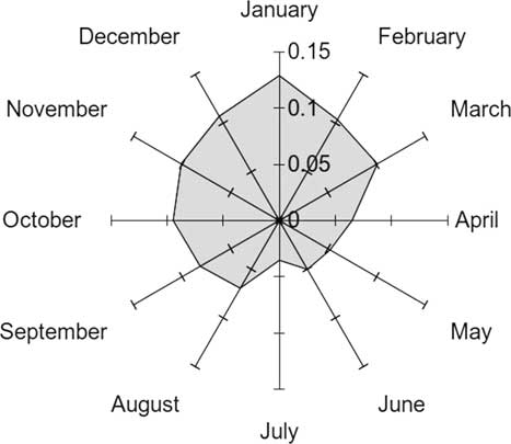
This research focused on the genetic analysis of lambing distribution throughout the year in the Ripollesa sheep breed. More specifically, analyses relied on the re-scaled day of lambing from 1 January (0) to 31 December (regular years, 2π–2π/365; leap years, 2π–2π/366). A total of 26 005 records from 4764 Ripollesa ewes were collected from 20 purebred flocks between years 1976 and 2017 (Figure 1). Only 23.6% of records from companion paper (Casellas et al., Reference Casellas, Martín de Hijas-Villalba and Id-Lahoucine2019) were retained for current genetic analyses due to more restrictive criteria in terms of pedigree information. Exclusively those ewes with known sire and dam and their first-generation relatives (i.e. mother and daughters) were included to prevent excessive incompleteness in the available genealogy. The pedigree file included 6537 individuals, 303 of them being sires contributing between 1 and 75 daughters with lambing data (mean, 15.4 daughters). Focusing on ewes, 2895 had known sire and dam, 1574 lacked information about their parents and 295 missed one parent.
Lambing distribution on a monthly basis in the Ripollesa sheep breed.

Heteroskedastic circular mixed model
The model considered was a straightforward extension of the canalization circular mixed model developed by Casellas et al. (Reference Casellas, Martín de Hijas-Villalba and Id-Lahoucine2019) on the basis of SanCristobal-Gaudy et al. (Reference SanCristobal-Gaudy, Elsen, Bodin and Chevalet1998) and Ibáñez-Escriche et al. (Reference Ibáñez-Escriche, Sorensen, Waagepetersen and Blasco2008a and Reference Ibáñez-Escriche, Varona, Sorensen and Noguera2008b). It relied on the von Mises distribution (Fisher, Reference Fisher1993) because (1) it wraps around the circle, and (2) approximates the wrapped normal distribution with the same number of parameters and a more tractable form (Breitenberger, Reference Breitenberger1963; Fisher, Reference Fisher1993). Assuming a set of n quantitative data (y) taken around a circular parametric space from 0 to 2π, the hierarchical structure of the model was stated as:
 $${\bf{y}} {\equals}{\bf{Xb}} {\plus}\mathop \sum\limits_{{\it j{\equals}1}}^{\it r} {\bf{Z}} _{{\it j}} {\bf{p}} _{{\it j}} {\plus}{\bf{Z}} _{{\it k}} {\bf{a}} {\plus}{\bf{e}} $$
where b, p j and a were systematic, permanent environmental and additive genetic effects with pertinent incidence matrices (X, Z j and Z k ), and e was the vector of residual terms. Note that r independent permanent environmental effects were assumed to guarantee model flexibility. Assuming a heteroskedastic structure on e, the joint posterior distribution of all unknown parameters was defined as
 $$\eqalign{{\it p} \left( {{\bf{b}} ,{\bf{\bbeta }} ,{\bf{p}} ,{\bf{\brho }} ,{\bf{a}} ,{\bf{\balpha }} ,{\bf{P}} ,{\bf{G}} \,\mid\,{\bf{y}} } \right)\cr \propto{\it p}\left( {{\bf{y}} \,\mid\,{\bf{b}} ,{\bf{\bbeta }} ,{\bf{p}} ,{\bf{\brho }} ,{\bf{a}} ,{\bf{\balpha }} } \right){\rm p}\left( {{\bf{b}} ,{\bf{\bbeta }} } \right)p\left( {{\bf{p}} ,{\bf{\brho }} \,\mid\,{\bf{P}} } \right){\it p}\left( {\bf{P}} \right)$$
 $${\it {\times}p}\left( {{\bf{a}} ,{\bf{\balpha }} \,\mid\,{\bf{A}} ,{\bf{G}} } \right){\it p}\left( {\bf{G}} \right)$$
where β, ρ and α were systematic, permanent environmental and additive genetic factors affecting the variance of the residual term (see below),
 ${\bf{p}} {\equals}\left[ {{\bf{p}} _{1}^{,} {\bf{p}} _{2}^{,} \,\ldots\, {\bf{p}} _{r}^{,} } \right]^{,} $
,
 $${\bf{\brho }} {\equals}\left[ {{\bf{\brho }} _{1}^{\prime} {\bf{\brho }} _{2}^{\prime} \,\ldots\, {\bf{\brho }} _{{\rm r}}^{\prime} } \right]^{,} $$
, P stored permanent environmental covariances between p and ρ terms, G stored additive genetic covariances between a and α terms, and A was the numerator relationship matrix (Wright, Reference Wright1922). The conditional distribution of y given all relevant parameters was a von Mises process as follows:
 $$\eqalign{{\it p} \left( {{\bf y}\,\mid\,{\bf{b}} ,{\bf{\bbeta }} ,{\bf{p}} ,{\bf{\brho }} ,{\bf{a}} ,{\bf{\balpha }} } \right) \cr {\equals}\mathop \prod\limits_{{\it i{\equals}}1}^{\it n} {{{\it e}^{{{\it e}^{{\left( {{\bf{x}} _{{\it i}} {\bf{\bbeta }} {\plus}\sum_{{\it j{\rm \equals}\rm 1}}^{\it r} {\bf{z}} _{{{\it i,j}}} {\bf{\brho }} _{{\it j}} {\plus}{\bf{z}} _{{{\it i,k}}} {\bf{\balpha }} } \right)}} {\rm cos}\left( {{\bf{y}} _{{\it i}} {\minus}\left( {{\bf{x}} _{{\it i}} {\bf{b}} {\plus}\sum_{{\it j{\equals}\rm 1}}^{\it r} {\bf{z}} _{{{\it i,j}}} {\bf{p}} _{{\it j}} {\plus}{\bf{z}} _{{{\it i,k}}} {\bf{a}} } \right)} \right)}} } \over {2{\rm \pi I}_{0} \left( {{\rm e}^{{\left( {{\bf{x}} _{{\it i}} {\bf{\bbeta }} {\plus}\sum_{{\it j{\equals}\rm 1}}^{\it r} {\bf{z}} _{{{\it i,j}}} {\bf{\brho }} _{{\it j}} {\plus}{\bf{z}} _{{{\it i,k}}} {\bf{\balpha }} } \right)}} } \right)}}$$
Note that x i , z i,j and z i,k were appropriate row vectors of incidence inherent to the ith circular record (y i ), π referred to the ratio of the circumference of a circle to its diameter, and I0(θ) was the modified Bessel function of order 0, that is:
 $${\rm I}_{{\rm 0}} \left( {\rm \rtheta } \right){\equals}\mathop \sum\limits_{{\it i{\equals}}0}^\infty {{\left( {0.{\rm 25\rtheta }^{2} } \right)^{{\it i}} } \over {\left( {{\it i\,\rm !\,}} \right)^{2} }}$$
The priors for permanent environmental and additive genetic effects were multivariate normal distributions (MVN):
 $$\eqalign{{\it p}\left( {{\bf{p}} ,{\bf{\brho }} \,\mid\,{\bf{P}} } \right) {\equals}\mathop \prod\limits_{{\it j{\equals}\rm 1}}^{\it r} {\it p}\left( {{\bf{p}} _{{\it j}} ,{\bf{\brho }} _{{\it j}} \,\mid\,{\bf{I}} _{{\it j}} \,\otimes\,{\bf{P}} _{{\it j}} } \right) \cr {\equals}\mathop \prod\limits_{{\it j{\equals}\rm 1}}^{\it r} {\rm MVN}\left( {\matrix{ {{\bf{0}} _{{\it j}} } \cr {\bf0_{{\it j}} } \cr } ,{\bf{I}} _{{\it j}} \,\otimes\,{\bf{P}} _{{\it j}} } \right)$$
and
 $${\it p}\left( {{\bf{a}} ,{\bf{\balpha }} \,\mid\,{\bf{A}} ,{\bf{G}} } \right){\rm {\equals}MVN}\left( {\matrix{ {{\bf{0}} _{{\it k}} } \cr {{\bf{0}} _{{\it k}} } \cr } ,{\bf{A}} \,\otimes\,{\bf{G}} } \right)$$
where for s
j
elements in p
j
and s
k
individuals in the pedigree file. Moreover, 0
j
was a s
j
× 1 vector of zeros, 0
k
was a s
k
× 1 vector of zeros, I
j
was a s
j
× s
j
identity matrix,
 $\,\otimes\,$
the Kronecker product, and G the matrix storing additive genetic variances (
 $\sigma _{a} ^{2} $
and
 $\sigma _{\balpha } ^{2} $
) and covariances (
 $\sigma _{{{\rm a\balpha }}} {\equals}\sigma _{{{\rm \balpha a}}} $
):
 $${\rm\bf G}{\equals}\left[ {\matrix{ {\sigma _{a} ^{2} } & {\sigma _{{{\rm a\balpha }}} } \cr {\sigma _{{\balpha a}} } & {\sigma _{\balpha } ^{2} } \cr } } \right]$$
The same rationale was applied to P j matrices of permanent environmental (co)variances (see Casellas et al., Reference Casellas, Martín de Hijas-Villalba and Id-Lahoucine2019 for details). Scaled inverse Wishart distributions were used as prior distributions for P j and G due to its computational simplicity (Van Tassell and Van Vleck, Reference Van Tassell and Van Vleck1996). Given our current lack of knowledge on circular data, a priori distributions of b were defined as flat between 0 and 2π:
 $${\rm p}\left( {\bf{b}} \right){\equals}{1 \over {{\rm 2\pi }}}({\rm if}\,{\bf{b}} {\repsilon}[0,2{\rm \pi }]\,{\rm and}\,{\rm 0}\,{\rm otherwise})$$
although an additional restriction was applied to guarantee that
 $0\leq {\bf{x}} _{{\it i}} {\bf{b}} {\plus}\mathop \sum\limits_{{\it j{\equals}\rm 1}}^{\it r} {\bf{z}} _{{{\it i,j}}} {\bf{p}} _{{\it j}} {\plus}{\bf{Z}} _{{\it k}} {\bf{a}} \leq {\rm 2\pi }$
.
The heteroskedastic mixed circular model assumed a hierarchic residual term which originated heterogeneous residual variance across lambing distribution records. In order to calculate heritability, a specific incidence of systematic and random effects (x*, z
j
* and z
k
*) must be assumed for the residual term (i.e.
 ${\epsilon}{\asterisk}{\rm {\equals}exp}\left( {{\bf{x}} {^\asterisk}{\bf{\bbeta }} {\plus}\mathop \sum\limits_{{\it j{\equals}\rm 1}}^{\bf{\it r}} {\bf{z}} _{{\it j}} {^\asterisk}{\bf{\brho }} _{{\it j}} {\plus}{\bf{z}} _{{\it k}} {^\asterisk}{\bf{\balpha }} } \right)$
). Within the context of the von Mises circular distribution, realized variance can be calculated as
 ${\rm \sigma }^{2} {\rm {\equals}1{\minus}}{{{\rm I}_{1} \left( {{\rm {\epsilon}}{\asterisk}} \right)} \over {{\rm I}_{0} \left( {{\rm {\epsilon}}{\asterisk}} \right)}}$
, where
 $I_{0} \left( {{\epsilon}{\asterisk}} \right)$
and
 $I_{1} \left( {{\epsilon}{\asterisk}} \right)$
are modified Bessel functions of order 0 and 1, respectively (Fisher, Reference Fisher1993).
Analytical process
The analytical model included three systematic effects accounting for population mean, ewe age at lambing (<3, 3, 4, 5, 6 and >6 years), and lambing interval (first lambing, <210 days, between 210 and 239 days, between 240 and 329 days, and ⩾330 days). Permanent environmental sources of variation were flock-year-season (186 levels) and the environmental contribution of each ewe (4681 levels). Environmental influences from rams, if any, were implicitly absorbed by the flock-year-effect, although all flocks kept a large enough number of rams to guarantee that all ewes in heat could be effectively mounted (>1 ram/30 ewes). In order to account for different genetic backgrounds in founder individuals, herd-by-year genetic groups were considered when constructing A (Westell et al., Reference Westell, Quaas and Van Vleck1988).
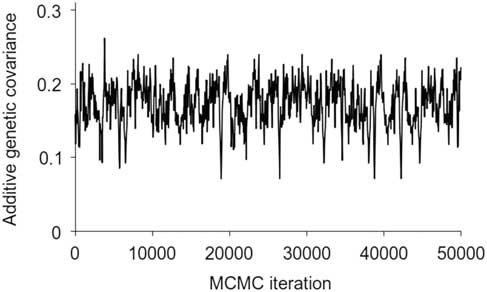
All the unknown parameters in the model were sampled from their marginal posterior distributions by appropriate Gibbs sampling (Gelfand and Smith, Reference Gelfand and Smith1990) or Metropolis-Hastings (Metropolis et al., Reference Metropolis, Rosenbluth, Rosenbluth, Teller and Teller1953). Three independent Monte Carlo Markov chains with 510 000 iterations were run for each analysis, where the first 10 000 iterations were discarded as burn-in. The suitability of the length of the burn-in period was evaluated by both visual inspection (Figure 2) and Raftery and Lewis’ (Reference Raftery and Lewis1992) method on the sampling path of
 $\sigma _{\balpha } ^{2} $
. A total of 10 000 samples of model parameters were saved from each chain with a lag interval of 50 iterations.
Markov chain Monte Carlo (MCMC) sampling path of the additive genetic covariance during the first 50 000 iterations after the burin-in period of the analysis of lambing distribution in the Ripollesa sheep breed.

Results and discussion
Lambing distribution must be viewed as a typical example of a circular trait with economic relevance in the meat sheep industry (Chemineau et al., Reference Chemineau, Bodin, Migaud, Thiéry and Malpaux2010). Nevertheless, difficulties with the statistical analysis of circular data have systematically impaired the study of this trait and its potential inclusion into current breeding schemes. As an example, lambing distribution was suggested as repeatable and heritable more than 30 years ago (Ricordeau, Reference Ricordeau1982; Quirke et al., Reference Quirke, Hanrhan, Loughnane and Triggs1986; Al-Shorepy and Notter, Reference Al-Shorepy and Notter1997) nevertheless, successful examples of selection on lambing distribution or closely related traits are really scarce (Teyssier et al., Reference Teyssier, Canepa, Chemineau, Malpaux, Migaud and Bodin2002). This shortage must be softened by the development of a circular generalized linear regression model within a Bayesian context by Mulder and Klugkist (Reference Mulder and Klugkist2017), which has been adapted to the animal breeding paradigm by Casellas et al. (Reference Casellas, Martín de Hijas-Villalba and Id-Lahoucine2019). In fact, previous estimates reported in the Ripollesa sheep breed (Casellas et al., Reference Casellas, Martín de Hijas-Villalba and Id-Lahoucine2019) were the first available from an analysis of lambing distribution under a circular approach. Moreover, they evidenced a remarkable degree of heteroskedasticity influencing both systematic and permanent environmental sources of variation for lambing distribution.
Systematic sources of variation
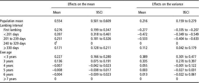
Apart from the population mean, only two systematic effects were included in the operational model, that is, lambing interval and ewe age. Estimates are shown in Table 1, but their interpretation must be cautious due to the circular parametric space. They were reported as departures from the population mean, except for the most abundant level that was arbitrarily fixed to 0. Furthermore, as circular analyses have infinite solutions with a 2π lag interval without impairing model fit (Fisher, Reference Fisher1993), the analytical model forced
 $0\leq {\bf{x}} _{{\it i}} {\bf{b}} {\plus}\mathop \sum\limits_{{\it j{\equals}\rm 1}}^{\it r} {\bf{z}} _{{{\it i,j}}} {\bf{p}} _{{\it j}} {\plus}{\bf{Z}} _{{\it k}} {\bf{a}} \leq {\rm 2\pi }$
to guarantee convergence. Within this context, the estimate for the ith systematic effect (
 $\widehat{{ b_{i} }}$
) in Table 2 must be viewed as the posterior mean of the shortest distance between population mean (μ) and lambings affected by the ith effect, although the complementary distance would also be plausible (i.e.
 ${\rm \mu {\minus}}\left( {{\rm 2\pi {\minus}}\widehat{{ b_{i} }}} \right)$
). This must be viewed as a major peculiarity during the analysis of circular data, because large systematic effects could be markedly underestimated without any kind of impact on model fit or complexity. The same uncertainty applies to the direction of the effect (i.e. positive or negative). This ambivalence originated in the lack of relevant information to anticipate the direction of systematic effects unless the systematic effect itself contributes some additional information to decipher its own direction around the circular parametric space.
Posterior mean and 95% credibility interval (95CI) of systematic effects on lambing distribution in the Ripollesa sheep breed

1 Estimates for 240 to 329 days of lambing interval and 7-year-old ewes and older were arbitrarily fixed to 0 to guarantee model identifiability.
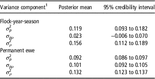
Posterior mean and 95% credibility interval of permanent environmental components for lambing distribution in the Ripollesa sheep breed

1 σ p 2 (σ ρ 2)=direct (residual) permanent environmental variance; σ pρ =covariance between direct and residual permanent environmental effects.
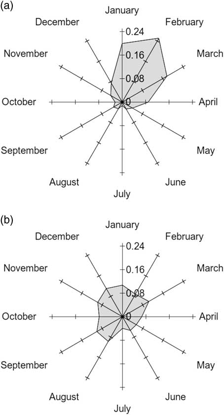
First lambing and short lambing intervals (<239 days) delayed lambing peak (<30 days), whereas a remarkable increase in the dispersion of lambing distribution was also reported (Table 1) when comparing with lambing intervals between 240 and 329 days. On the other hand, ewe age showed minimal differences for mature ewes from 4-year old, whereas youngest females tended to delay and concentrate the lambing peak (Figure 3). The retardation in lambing period for in 2-year-old females have been previous reported in wild sheep (Bon et al., Reference Bon, Dardaillon and Estevez1993).
Lambing distribution on a monthly basis for (a) young (<3 years old) and (b) old ewes (⩾7 years old) ewes of the Ripollesa sheep breed.

Permanent environmental effects
Both flock-year-season and ewe had relevant consequences on lambing distribution as permanent environmental effects (Table 2), although they were smaller than the additive genetic ones (see below). All variance terms (σ p 2 and σ ρ 2) placed their 95% credibility intervals far from zero, and the same happened for the permanent environmental covariance of permanent ewe, this originating an environmental correlation of 0.917. It must be highlighted that non-additive genetic contributions may be captured by the environmental ewe effect. On the other hand, the 95% credibility interval of the covariance for flock-year-season included the null estimate and thus, direct and residual flock-year-season effects must be considered as uncorrelated.
Additive genetic backgrounds
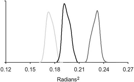
Figure 4 showed posterior distributions for additive genetic variance components derived from the heteroskedastic circular mixed model. The posterior mean for σ a 2 was 0.193 radians2 (i.e. σ a = 0.437 radians ~ 25 days), whereas σ α 2 reached 0.228 radians2, and 95% credibility intervals excluded the null estimate in both cases (Figure 4). Given that lambing distribution data was analyzed under a heteroskedastic circular mixed model, heritability changed across levels of systematic and random effects (Ros et al., Reference Ros, Sorensen, Waagepetersen, Dupont-Nivet, SanCristobal, Bonnet and Mallard2004). Heritability for lambing distribution ranged from 0.182 (lambing interval, ⩾330 days; ewe age,<3 years) to 0.278 (lambing interval, 201 to 239 days; ewe age, ⩾7 years). Note that these estimates assumed a null contribution from permanent environmental (ρ=0) and additive genetic effects (α=0), this being the expected average contribution from all this sources of variation (see a priori multivariate normal distributions assumed in the ‘Materials and methods’ section). These values corroborated the existence of genetic background for lambing distribution in the Ripollesa breed, agreeing with previous researches performed on linear models (Ricordeau, Reference Ricordeau1982; Quirke et al., Reference Quirke, Hanrhan, Loughnane and Triggs1986).
Posterior density of direct additive genetic variance (black line), residual additive genetic variance (dark gray) and genetic covariance (fair gray) for lambing distribution in Ripollesa ewes.

It must be noted that genetic selection applied on a or α should have completely different consequences on lambing distribution. Active selection for high and positive (high and negative) breeding values in vector a must delay (advance) the lambing season, this moving the lambing peak. In contrast, selection for high and positive (high and negative) breeding values in vector α should increase seasonality and concentrate lambings in a shorter lambing season (reduce seasonality and provide wider lambing seasons). Note that this rationale relies on the additive genetic effect inherent to the residual term, and therefore allows to increase or reduce the residual dispersion pattern. Within this context, this analysis lay the foundations of genetic selection for low-seasonal ewes. Indeed, non-zero σ α 2 agrees with selection response for fall-lambing previously reported by Al-Shorepy et al. (Reference Al-Shorepy and Notter1997), as well as the marked differences in terms of seasonality-related patterns when comparing breeds from northern and southern Europe (Wheeler and Land, Reference Wheeler and Land1977; Forcada et al., Reference Forcada, Abecia and Sierra1992).
The covariance between a and α was 0.171. These values generated a high genetic correlation of 0.814, with a 95% credibility interval ranging from 0.503 to 0.964. The positive and relevant relationship between a and α for lambing distribution in the Ripollesa breed suggested that genetic selection for low seasonality must also advance lambing season. The rationale behind this high and positive correlation must be linked to the current lambing peak (Figure 1). As noted by Wheeler and Land (Reference Wheeler and Land1977) and Forcada et al. (Reference Forcada, Abecia and Sierra1992), most of the ewes lambed at the beginning of the lambing season in northern hemisphere; if moved backwards (i.e. smaller a values), most lambings would advance to counter-season months, they implicitly involving lower reproductive seasonality (i.e. larger variance for lambing distribution and smaller α values). On the other hand, a delay in lambing peak (i.e. larger a values) may result with higher sensitivity to season-related factors and their influences on the reproductive function. As a consequence, a narrower lambing season would be anticipated (i.e. larger α values). Although this results cannot be directly extrapolated to all sheep breeds worldwide, current animal breeding programs must be aware of the relevance of heteroskedastic circular mixed models for genetic evaluation purposes.
Acknowledgements
The authors are indebted to the Ripollesa breed society for contributing field data. M.M.d.H.-V. was supported by a scholarship (BES-2017-080596) from the Ministerio de Economía, Industria y Competitividad of Spain’s government (Madrid, Spain).
Declaration of interest
The authors do not have conflicts of interest with the subject matter of this manuscript.
Ethics statement
Animal Care and Use Committee approval was not necessary for this study because analyses were performed on existing field data obtained under standard farm management from commercial breeders. Both productive and reproductive data were collected by the stockbreeders themselves and administrated by the Ripollesa Breed Society (Associació Nacional de Criadors d’Oví de Raça Ripollesa (ANCRI), Monells, Spain) within the context of its yield recording program.
Software and data repository resources
Data and model used for the purpose of this study are not deposited in an official repository.