

Dual-process theories characterize decision making as a product of two interacting cognitive systems (Evans, Reference Evans2008; Gawronski & Creighton, Reference Gawronski, Creighton and Carlston2013). Depending on the research area and focus, the two systems have been described, for example, as automatic and controlled (Schneider & Shiffrin, Reference Schneider and Shiffrin1977), intuitive and analytic (Hammond, Reference Hammond1996), heuristic and analytic (Evans, Reference Evans2006), or affective and deliberate (Loewenstein, O’Donoghue, & Bhatia, Reference Loewenstein, O’Donoghue and Bhatia2015; Stanovich & West, Reference Stanovich and West2000), and Kahneman and Frederick (Reference Kahneman, Frederick, Gilovich, Griffin and Kahneman2002) simply termed them Systems 1 and 2. In line with this literature in cognitive psychology, neuroscience research also suggests that the human mind is composed of multiple systems that approach decisions in distinct ways: A fast, habit-based system, and a slow, goal-directed system (see reviews by Dolan & Dayan, Reference Dolan and Dayan2013; Rangel, Camerer, & Montague, Reference Rangel, Camerer and Montague2008).
Despite the converging evidence on the existence of the two separate systems, the field currently lacks formal mathematical models that can account for the dynamic aspect of the interactions between the two systems. On the one hand, the majority of dual process models are verbal models that simply describe the two systems and their interplay, without generating testable quantitative predictions. On the other hand, in the few cases where formal models for decision making have been proposed (Loewenstein et al., Reference Loewenstein, O’Donoghue and Bhatia2015; Mukherjee, Reference Mukherjee2010), utilities are often modeled as weighted combinations of two decision values independently assigned by Systems 1 and 2. These models are silent regarding the timing of the two systems, which is nonetheless a core feature of verbal models on dual process theories. As many of these theories suggest, the two systems operate in a sequential manner, and the slower System 2 modifies the response of the fast System 1. Recently, Diederich and Trueblood (Reference Diederich and Trueblood2018) proposed a dynamic stochastic modeling framework of dual process theory, which provides an account of the timing and interaction of the two systems. The framework is based on research using multi-stage sequential sampling models (Diederich, Reference Diederich1997, Reference Diederich2016) and was applied to risky choices presented in gain and loss frames (Diederich & Trueblood, Reference Diederich and Trueblood2018).
In the current paper, we extend the framework to apply it to intertemporal choices, i.e., choices between rewards and punishments at different points in time. For instance, the decision maker can be asked to choose between an amount x1 available immediately, and an amount xt available with a delay of time t (x1 < xt). A range of behavioral and brain-imaging studies support a dual-process account of intertemporal choices, such that System 1 has a tendency to choose immediate rewards over delayed rewards, and this tendency may be modified by the subsequent System 2 (Figner et al., Reference Figner, Knoch, Johnson, Krosch, Lisanby, Fehr and Weber2010; Hare, Camerer, & Rangel, Reference Hare, Camerer and Rangel2009; Peters & Büchel, Reference Peters and Büchel2011). For example, large-scale behavioral studies demonstrate that individuals with better cognitive control abilities (and thus influenced by System 2 more) tend to be more patient (Burks, Carpenter, Goette, & Rustichini, Reference Burks, Carpenter, Goette and Rustichini2009; Shamosh et al., Reference Shamosh, DeYoung, Green, Reis, Johnson, Conway and Gray2008). fMRI evidence also suggests that there are two neural valuation systems with different discount rates (McClure, Ericson, Laibson, Loewenstein, & Cohen, Reference McClure, Ericson, Laibson, Loewenstein and Cohen2007; McClure, Laibson, Loewenstein, & Cohen, Reference McClure, Laibson, Loewenstein and Cohen2004), which is consistent with the idea that System 1 discounts delayed rewards more than System 2. On the modeling side of intertemporal choices, however, only a few notable dual process models have been proposed (see Fudenberg & Levine, Reference Fudenberg and Levine2006; Loewenstein et al., Reference Loewenstein, O’Donoghue and Bhatia2015). None of them provide a formal specification regarding the dynamics of the interplay of the two systems. More recently, Zhao, Diederich, Trueblood, and Bhatia, (2019) attempt a pseudo-dual process model of intertemporal choice using single-stage sequential sampling models. They did not explicitly model the dynamics of System 1 but permit automatic biases to influence decisions both prior to and during the preference integration process (which is assumed to occur in System 2). In the current paper, we keep the sequential sampling framework but switch to a two-stage model – one stage per system – which allows us to model the timing and interplay of the two systems explicitly.
In the following sections, we first discuss the modeling framework, and then discuss its qualitative and quantitative predictions.
Model framework description
We begin describing the general framework of the dynamic stochastic model followed by qualitative predictions (cf. Diederich & Trueblood, Reference Diederich and Trueblood2018).
In line with Decision Field Theory (DFT, Busemeyer & Townsend, Reference Busemeyer and Townsend1993) and Multiattribute Decision Field Theory (MDFT, Diederich, Reference Diederich1997), we assume that decisions are based on a preference state, denoted P (t), presenting the relative preference strength for choosing one option (here, the immediate reward, RI) over another option (here, the delayed reward, RD) at time t. Assume that a positive value of P(t) represents a momentary preference in the direction of favoring option RI whereas a negative value of P(t) represents a momentary preference in the direction of favoring option RD Preference strength is updated from one moment, t, to the next, (t + τ) by an input valence, V(t) reflecting the momentary comparison of consequences produced by imagining the choice of either option RD or RI with  $V\left( t \right) = {V_{{R_I}}}\left( t \right) - {V_{{R_D}}}\left( t \right)$, where
 ${V_{{R_D}}}\left( t \right)$ is the momentary valence for the delayed reward and
 ${V_{{R_I}}}\left( t \right)$ for the immediate. The valence fluctuates because the decision maker’s attention switches back and forth to anticipated consequences. For dual processes, we assume that the input valence also depends on the system i, where i = 1, 2, in which the decision maker (DM) is operating.
The preference process can be described by the following equation
 $$P\left( {t + \tau } \right) = P\left( t \right) + {V_i}\left( {t + \tau } \right),$$
where τ is a small time unit and Vi(t) is the system specific valence input. The mean valence, when comparing the choice options and operating within system i, is E[Vi(t)] = μit. The parameter μi called the drift rate, indicates the direction and strength of preference towards choosing option RD or RI .
In particular for μi > 0, preference is directed towards choosing option RI whereas for μi < 0, it is directed towards choosing RD . The larger the absolute value of μi the stronger is the preference for the given choice option. For µ = 0, the DM is indifferent between the two choice options. The preference process stops and a final decision is made as soon as the preference state exceeds a decision threshold or boundary: If  $P\left( t \right) &lt; {\theta _{{R_D}}} &lt; 0$, the DM chooses the delayed reward RD and if
 $P\left( t \right) &gt; {\theta _{{R_I}}} &gt; 0$, the DM chooses the immediate reward RI. The decision threshold is assumed to be set prior to the decision task by the DM and depends, among other things, on the time available for a decision. Under short time limits, the boundaries are assumed to be smaller than under no time limits.Footnote 1 Thus, the probability of choosing the immediate reward RI over the delayed reward RD is determined by P(t) reaching the positive threshold before reaching the negative threshold.
Two-stage model and its predictions
A widely made assumption is that System 1 (intuitive, affective) operates first before processing is taken over by System 2 (rational, deliberate) (e.g. Evans, Reference Evans2008, for an overview). That means, at some point in time, the DM moves from operating mostly in System 1 to operating mostly in System 2. This is a serial or two-stage dual process model. It is also possible that the two systems interact simultaneously (a one-stage process). However, here we concentrate on the two-stage model and its predictions only. We explore the simultaneous assumption in future research.
The two-stage model is illustrated in Figure 1. Each panel describes a different situation explained below. Within each figure, a single colored trajectory represents the preference accumulating (updating) process for one trial, i.e., when choosing between the delayed and immediate reward. The black trajectories (straight lines) are the expected values of the all possible trajectories with slopes given by the drift rates μ1 (before t 1) and µ 2 (after t 1), which represent the mean preference towards options RD and RI. The upper boundary  ${\theta _{{R_I}}}$ refers to the criterion for choosing the immediate reward RI, and the lower boundary
 ${\theta _{{R_D}}}$ to the criterion for choosing the delayed reward RD. In this illustration, we assume that when operating in System 1, preference is directed towards the immediate reward (myopic view).Footnote 2 This is reflected by a positive drift rate, i.e. μ1 > 0. At time t 1, operating switches from System 1 to System 2.Footnote 3 In the examples, the drift rate for the process in System 2 depends on the (discounting) function that the DM might employ. Without specifying the functions yet (see below), a negative drift rate, μ2 < 0, means that the DM evaluates the delayed reward higher than the immediate one. Panel A shows this situation. When operating in System 2, the preference for choosing the immediate over the delayed reward reverses after t 1. When the DM, operating in System 2, is indifferent between choosing the immediate and the delayed reward, the drift rate is μ2 = 0 (panel B). The remaining two panels describe situations that may be less common. Operating in System 2, the DM still prefers the immediate reward but the preference strength is less strong than before, i.e. 0 < μ2 < μ1 (panel C). Note that situation B is a special case of C as μ2 < μ1. Finally, the DM’s preference strength for choosing the immediate reward even increases when operating in System 2, described by the drift rate 0 < μ1 < μ2. Note that, the process can stop at any time while operating in System 1 or in System 2 to initiate a response.
Two-stage Dynamic–Stochastic Dual Process Model.
Each stochastic (colored) trajectory symbolizes the preference accumulation for one trial (four trials in each panel). Once a trajectory hits a boundary, i.e., the criterion for choosing the immediate reward  $\left( {{\theta _{{R_I}}}} \right)$ or the delayed one
 $\left( {{\theta _{{R_D}}}} \right)$, a choice is made in favor of that option. The black trajectories (straight lines) indicate the expected value of all trajectories and thereby the mean preference directed towards either criterion. When operating in System 1, preference is directed towards choosing RI (μ1 > 0). At t 1, attention switches to System 2 and A: preference is directed towards choosing RD (μ2 < 0 < μ1). B: the DM is indifferent between choosing RI and RD (0 = μ2 < μ1). C and D: preference is directed towards RI but with different strength.

Following Loewenstein et al. (Reference Loewenstein, O’Donoghue and Bhatia2015), we call a preference for the immediate reward myopic behavior and the magnitude thereof a myopic effect.
The two-stage model makes predictions about the size of the myopic effect due to the dynamic of the two systems and more specific predictions when specifying the shape of the discounting function, in particular with respect to the relation between choice probabilities and choice response times.
Prediction 1: Given that System 1 is driven by a myopic view (preferring the immediate reward) and System 2 by a deliberate view (depending on the discounting factor/function as shown in panels A, B, and C), then the size of the myopic effect is a function of the time the DM operates in System 1.
When the DM switches to System 2 early on in the preference accumulation process, the decision is mainly based on the rational process and the myopic effect should be small. The longer the DM operates in System 1, the stronger the myopic effect is. Figure 2, panels A to C, illustrates this situation. Each of the four trajectories represents the preference accumulating process for one trial, i.e. to make a choice between the immediate and delayed reward. In panel A, the DM spends little time in System 1 before switching to System 2. No decision has been made during that time and the decision is mainly based on System 2. This does not mean that System 1 has no influence on the subsequent processing in System 2: The drift rate (indicated by the straight black line) is indeed negative (preference for the delayed reward) but it is shifted towards the boundary  ${\theta _{{R_I}}}$ for choosing the immediate reward. Only if the DM operates solely in System 2, then no myopic effect occurs. In panel C, the DM operates in System 1 for quite some time (in the illustration, three times as long as in panel A) and preference accumulation becomes large enough to initiate a response in favor of the immediate reward before System 2 was even involved. Thus, extending the operating time in System 1 leads to more trials being finished within System 1, which in turn enlarges the myopic effect.
Two-Stage Dynamic–Stochastic Dual Process Model.
Each stochastic (colored) trajectory symbolizes the preference accumulation for one trial. Once a trajectory hits a boundary, i.e., the criterion for choosing the immediate reward  $\left( {{\theta _{{R_I}}}} \right)$ or the delayed one
 $\left( {{\theta _{{R_D}}}} \right)$, a choice is made in favor of that option. The (black) trajectories (straightlines) indicate the expected value of all possible trajectories, i.e., the mean preference directed towards either criterion. When operating in System 1, preference is directed towards choosing RI (μ1 > 0). At t 1, attention switches to System 2 and preference is directed towards choosing RD (μ2 < 0 < μ1). A, B, C: Increasing times spent operating in System 1 before switching to System 2. D: The same situation as in B but with decreased boundaries/decision criterion. The criterion is set by the DM and may depend on, for instance, time constraints.

Prediction 2: Given that System 1 is driven by a myopic view (preferring the immediate reward) and System 2 by a deliberate view (depending on the discounting factor/function as shown in Figure 1, panels A, B, and C) then the size of the myopic effect is a function of the time (limit) the DM has for making a choice.
Recall that the decision criterion set by the DM is a function of time limits. With shorter time limits the criterion is set smaller. With a smaller criterion, more choice responses are initiated earlier. Because System 1 precedes System 2, more choices are made while operating in System 1. Therefore, more choices are driven by System 1 and then myopic effect is larger under short deadlines. Figure 2, panels B and D, illustrates this situation. As before, each of the trajectories represents the preference accumulation process for one trial, i.e. to make a choice between the delayed and immediate reward. The simulated trajectories are identical in both panels. In panel B the choice criteria are large, i.e. the DM is not under time pressure. Panel D reflects the situation in which the DM is under time constraints. The criteria are smaller and a decision is reached sooner. In this example two choices are made early on in favor of the immediate reward (the trajectories reached the criterion  ${\theta _{{R_I}}}$). Note that, these two trajectories move down towards the criterion choosing the delayed reward,
 ${\theta _{{R_D}}}$ when more time is given, i.e, when the criteria are larger. We cannot infer from the illustration which boundary they will reach, but the more time available for operating in System 2, the less influential are the preference states accumulated in System 1.Footnote 4
The scenarios presented in Figure 1 span a wide range of patterns about how preferences can be built in the two systems. Indeed, we can even add those situations in which the DM ignores the delay in the first stage and only considers the rewards. In this case, the drift rate is negative in the first stage µ1 < 0; and the drift rate in System 2 (µ2) can be positive or negative (or even zero), depending on the DM’s preference function as discussed above. Even if this sounds very flexible, the two-stage dual process model makes predictions with respect to the choice probability/decision time patterns that provide a strong restriction to the model. The predictions are generic to the two-stage model per se and are not specific to the intertemporal choice situation.
Prediction 3A: Given that the mean valences (drift rates) in both systems do not point in different directions (as shown in Figure 1, panels B, C, and D) then the following patterns hold:
• If the mean valence in System 1 is larger (in absolute value) than in System 2 (panels B and C: 0 ≤ µ2 < µ1 or, not shown, μ1 < µ2 < 0), then the two-stage model always predicts faster mean response time to the more frequently chosen alternative.
• If the mean valence in System 1 is smaller (in absolute value) than in System 2 (panel D: 0 ≤ µ1 < µ2 or, not shown, µ2 < µ1 < 0), then the two-stage model always predicts faster mean response times to the less frequently chosen alternative.
The psychological interpretation for the latter is that if a less favorable alternative is chosen in System 1, here the delayed reward, then the answer tends to be fast, before later on in System 2 the mean valence for the more favorable option, here the immediate reward, even increases.
The choice-probability/choice-response patterns become more complex when mean valences of the two systems favor different options (i.e. have different signs). However, the patterns remain consistent (Diederich & Oswald, Reference Diederich and Oswald2014). In particular:
Prediction 3B: Given that the mean valences (drift rates) in both systems point in opposite directions (as shown in Figure 1, panel A), then the following patterns hold:
• Preference reverses with increasing time spent operating in System 1. That is, the probabilities for choosing one alternative change from below (above) 0.5 to above (below) 0.5 as operating time in System 1 increases.
• The larger the mean valence in System 1 is as compared to System 2 (absolute values), the sooner the reversal occurs as a function of operating time in System 1.
• When the mean valence in System 1 is larger (absolute value) than in System 2, then the more frequently chosen alternative is faster after the preferences reversal.
• When the mean valence in System 1 is smaller than in System 2, then the less frequently chosen alternative is faster after the preferences reversal.
That is, we observe the same patterns as before after the probabilities crossed (0.5), and the reverse patterns before the probabilities crossed. This will become clear when considering quantitative predictions. Therefore, the next step is to specify what determines the valences in each system, i.e. what drives the process towards choosing the immediate RI or delayed RD reward when operating in the two systems, and how this can be quantified.
Quantitative predictions of dual process models
Our framework allows us to test hypotheses about the functional forms of Systems 1 and 2 as well as the dynamic interaction of these two systems. As an example, we take a simplified version of the model proposed by Loewenstein et al. (Reference Loewenstein, O’Donoghue and Bhatia2015) for intertemporal choice. It is static and deterministic, and although the model is motivated as a dual-process approach (affective versus deliberate), behavior is determined by a single “objective” function, V(R), of the rewards R (Loewenstein et al., Reference Loewenstein, O’Donoghue and Bhatia2015, p. 60).
According to Loewenstein et al. (Reference Loewenstein, O’Donoghue and Bhatia2015), preferences in System 1 are constructed according to a motivational function M(R, a), which incorporates a variable a that captures the intensity of affective motivations (Loewenstein et al., Reference Loewenstein, O’Donoghue and Bhatia2015, p. 59), and is weighted by a function h(W, σ) that reflects the willpower strength W and cognitive demands σ. As in Diederich and Trueblood (Reference Diederich and Trueblood2018), we label the model as MWC (Motivation weighted by Willpower and Cognitive demand). For simplicity, we assume two rewards only, one immediate and one delayed. With RD indicating the payoff received at time TD, the affective system motivational function (System 1) is defined as(2)
 $$M\left( {R,a} \right) = {R_I} + \exp \left( { - {\delta _A}\left( a \right) \cdot {T_D}} \right) \cdot {R_D}$$
where δA(a) is the discounting factor of an exponential discounting function for the affective system. Increased affective intensity a implies a smaller δA(a) (Loewenstein et al., Reference Loewenstein, O’Donoghue and Bhatia2015, p. 62). M(R, a) is weighted by h(W, σ); the form of this function is not specified in Loewenstein et al. (Reference Loewenstein, O’Donoghue and Bhatia2015) but is meant to be decreasing in W and increasing in σ.
Preferences in System 2 are defined as
 $$U\left( R \right) = {R_I} + \exp \left( { - {\delta _D} \cdot {T_D}} \right) \cdot {R_D}$$
where δD is the discounting factor of an exponential discounting function for the deliberate system with
 $${\delta _A}\left( a \right) &lt; {\delta _D}.$$
The model by Loewenstein et al. (Reference Loewenstein, O’Donoghue and Bhatia2015) assumes that the functions as stated in Eq. 2 and Eq. 3 operate simultaneously, and the subjective value 𝒱(R) of an option is the sum of both processes. That is,
 $${\cal V}\left( R \right) = U\left( R \right) + h\left( {W,\sigma } \right) \cdot M\left( {R,a} \right).$$
Typically, a choice is based on both systems but choices made solely on System 1 or System 2 are also possible (Loewenstein et al., Reference Loewenstein, O’Donoghue and Bhatia2015, p.58). However, no rule is provided for the circumstances when this can happen.
In the following, we show how the (simplified) affective and deliberate system components can be incorporated in the dynamic-stochastic dual process model. We assume that preference evolves in System 1 and System 2 by comparing the consequences when choosing the immediate I and the delayed D option, producing valence values VI(t) and VD(t) respectively, at any moment in time. Because W and σ and the functional form of h(W, σ) are not specified, we set h(W, σ) := h, a constant, and δA(a) : = δ1 as the discounting factor for System 1. Furthermore, we assume that the expected values of the valences are related to the MWC values such that for System 1,  $E\left[ {{V_{{1_I}}}\left( t \right)} \right] = h \cdot {R_I} \cdot t$ for the immediate reward and
 $E\left[ {{V_{{1_D}}}\left( t \right)} \right] = h \cdot \exp \left( { - {\delta _1} \cdot {T_D}} \right) \cdot {R_D} \cdot t$ for the delayed reward, resulting in a mean difference in valence (which defines the drift rate) of
 $${\mu _1} = h \cdot \left[ {{R_I} - \exp \left( { - {\delta _1} \cdot {T_D}} \right) \cdot {R_D}} \right].$$
With the same reasoning and relabelling δD into δ2, operating in System 2 produces a mean difference in valence with
 $${\mu _2} = {R_I} - \exp \left( { - {\delta _2} \cdot {T_D}} \right){R_D}.$$
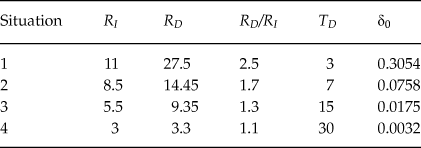
Obviously, Eq. 5 and Eq. 6 have the same functional form; the drift rates for System 1 and System 2, however, are different with δ1 < δ2 (Loewenstein et al., Reference Loewenstein, O’Donoghue and Bhatia2015). Note that, this assumption is in accordance with the scenarios presented in Figure 1 panels A, B, and C, but not with D. μ1 may be further scaled by h.Footnote 5 To demonstrate the quantitative predictions of the model, we use a subset of the stimulus values from Zhao et al. (Reference Zhao, Diederich, Trueblood and Bhatia2019). In their study, the immediate rewards were $3, $5.5, $ 8.5, and $11; the time delays TD were 3, 7, 15, and 30 days; and multipliers for the delayed reward, RD/RI, were 1.1, 1.3, 1.7, and 2.5 such that the delayed reward amounts were greater than the immediate reward amounts for each choice pair. In particular, we take four choice situations out of 64 as shown in Table 1:
Subset of Stimulus Values used by Zhao et al. (Reference Zhao, Diederich, Trueblood and Bhatia2019)

Note: RI indicates the immediate rewards; RD the delayed rewards; RD/RI the multipliers for the delayed rewards; TD the time delay, and δ0 the discount factor for an indifference judgment. The values are chosen such, that 1) all values appear once and 2) δ0 covers the entire range of possible discount factors (min: 0.0032; max: 0.3054).
To investigate the predictions quantitatively, we need to select a set of parameters. We proceed as follows. For making the predictions for Situations 1 to 4 in Table 1 comparable, we first determine the discounting factor in System 2 assuming indifference between choosing the immediate and the delayed reward. Labelling this factor as δ0 and solving the equation RI = exp(−δ0 · TD) ·RD for δ0 yields values listed in Table 1, last column. For those cases, μ2 = 0 (see Figure 1, panel B, System 2). The δ0 values are then taken as the base for modifying the direction of the preference towards an immediate and a delayed reward such that the new values are proportional to the base values. That is, we multiply δ0 by α1 in System 1 and by α2 in System 2 with α1 < α2 to eventually produce different drift rates (mean valences) towards the immediate and delayed reward. Thus, Eqs. 5 and 6 become
 $${\mu _1} = h \cdot \left[ {{R_I} - \exp \left( { - {\delta _0} \cdot {\alpha _1} \cdot {T_D}} \right) \cdot {R_D}} \right]$$
and
 $${\mu _2} = {R_I} - \exp \left( { - {\delta _0} \cdot {\alpha _2} \cdot {T_D}} \right){R_D},$$
respectively, where α1 and α2 are the only free parameters. For the demonstrations here, α1 is set to 0.99, 0.96 or 0.9 for System 1 and α2 to 1, 1.01, or 1.1 for System 2. h is set to 0.1 to 2 in steps of 0.1. Furthermore, for Prediction 1, the decision thresholds θI and θD are set to  ${\theta _{{R_I}}} = - {\theta _{{R_D}}} = 15$; for Prediction 2, the thresholds are set to ±10, ±15, and ±20. The time operating in System 1 before switching to System 2 begins with 2 arbitrary time units and is increased in steps of 2 time units.Footnote 6
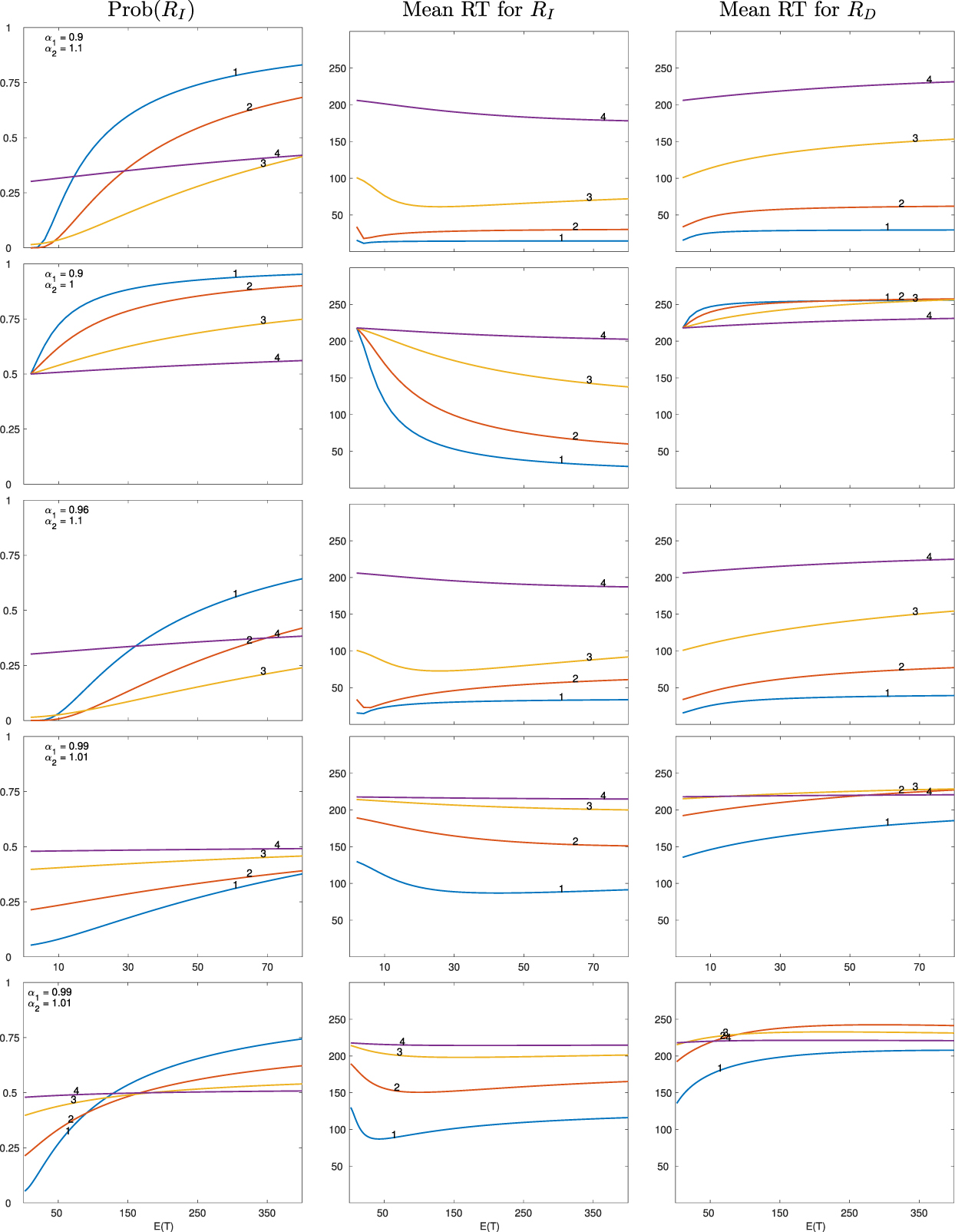
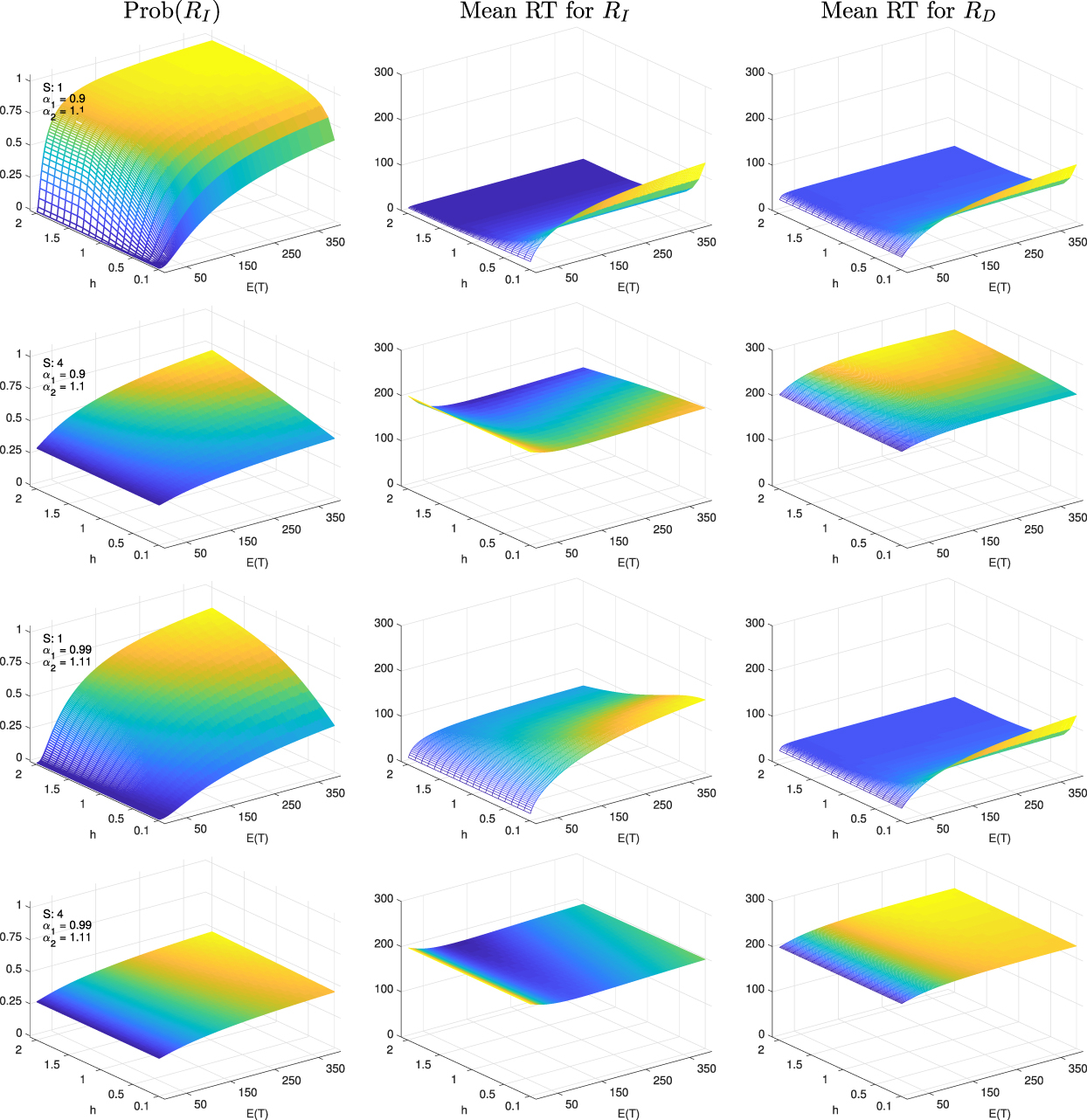
Figure 3 shows the predictions for h = 1. Figure 5 shows predictions for h ranging from 0.1 to 2 in steps of 0.1 for a subset of parameters and situations shown in Table 1. The rows in each figure show the predictions for various α parameter combinations found in the left corner of the left column panels. Columns refer to the probability of choosing the immediate reward RI (left); mean choice response times for choosing the immediate reward RI (middle); and mean choice response times for choosing the delayed reward RD (right). We address each panel in the figure according to its position; the first number refers to the row, the second to the column (for instance, Panel (3,1) displays the probabilities to choose RI with α1 = 0.96 and α2 = 1.1). The Labels 1 to 4 in the graphs correspond to the choice situations as described in Table 1. We now turn to the predictions.
Predictions of the dynamic two-stage dual process model for choice probabilities and choice response times as a function of the expected time E(T) spent operating in System 1 before switching to System 2. The time units are arbitrary. The range is the same for panels in Rows 1 to 4. h(W, σ) = 1; θ = ±15 (arbitrary unit); the specific α parameters are presented in the upper left corner of the panels in the first column. Rows 4 and 5 present identical parameters but the range of E(T) differs.

Prediction 1: Recall that Prediction 1 basically says that the longer the DM operates in System 1 the more is the decision influenced by that system (affective system). That is, given that System 1 is driven by a myopic view (preferring the immediate reward) then the size of the myopic effect increases with increasing time spent in System 1.
Consider the choice probabilities first (first column of Figure 3). For any parameter combination, the probability for choosing the immediate reward increases as a function of increasing time operating in System 1 in accordance with Prediction 1. The shape of the function depends highly on the underlying discounting factors for both systems. In particular, in Panel (1,1), both α parameters are equally apart from the neutral (indifference) discounting factor δ0 and relatively large. Switching immediately (t 1 small) to System 2 increases the probability to choose RD. However, with increasingly more time spent operating in System 1, the probability for choosing RD increases considerably. In Panel (2,1), the drift rate for System 1 is the same as in Panel (1,1), i.e., an inclination to choose RI, but when operating in System 2, the DM is now indifferent, μ2 = 0 and smaller in absolute value than in Panel (1,1). Spending more time in System 1 increases the preference to choose RI even more, less evidence for choosing RD when operating in System 2 as compared to Panel (1,1). In Panel (3,1) the mean difference in valence for choosing RI while operating in System 1 decreased (the distance to δ0 decreased and the overall preference strength for choosing RI is lower). Operating in System 2 provides the same strength for choosing RD as in Panel (1,1). That is, the preference for choosing RI as a function of time spending operating in System 1 is less strong than shown in Panel (1,1). Panels (4,1) and (5,1) show the situation when the discounting factors are relatively close to δ0. The parameters for both examples are identical. However, to show the convergence of the process, the time range for switching from operating in System 1 to System 2 has been increased in Panel (5,1). That is, the model predicts that the DM needs to operate in System 1 considerably longer to choose the immediate reward when the myopic view is weak. Without going in any details of the response times yet (Prediction 3), it is clear from the figure, that the mean response times are different for choosing RI and RD.
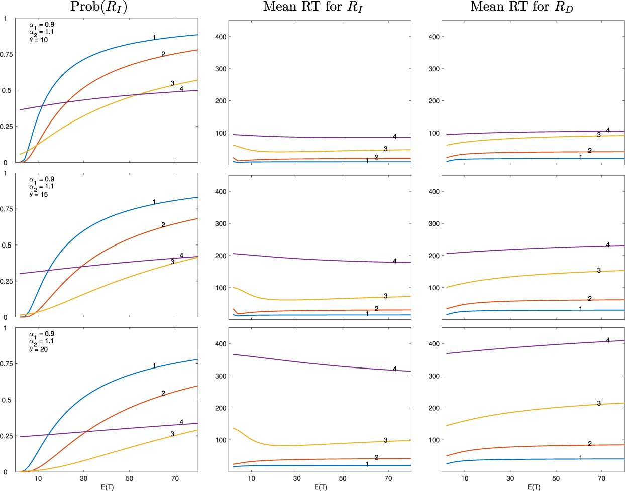
Prediction 2: Prediction 2 is concerned with the overall time for making a decision. Given that System 1 is driven by a myopic view (preferring the immediate reward), then the size of the myopic effect is a function of the time (limit) the DM has for making a choice. That is, the lower the boundary is, the more decisions are made while operating in System 1. Note that this relies on the assumption that operating in System 1 occurs before operating in System 2. Figure 4 shows the predictions for three different θ: θ = ±10 in Row 1, θ = ±15 in Row 2, and θ = ±20 in Row 3. The α parameters are set to α1 = .9 and α2 = 1.1, the same parameters as in Figure 3, Row 1. Note that, the scale for the response times are different in both figures to account for the longer mean response times when θ increases. Obviously, the probabilities for choosing the immediate reward as a function of t 1 are similar in shape. The magnitude of the probabilities, however, depends on the criterion θ (column 1). With increasing boundaries (from top to bottom), the influence of System 1 on the final decision decreases, given all remaining parameters being the same. Note that the overall time for making a decision increases as the boundary increases.
Predictions of the dynamic two-stage dual process model for choice probabilities and choice response times as a function of the expected time E(T) spent operating in System 1 before switching to System 2 for three different decision criteria θ : ±10, ±15 , and ±20. The units are arbitrary. h(W, σ) = 1; the specific α parameters are presented in the upper left corner of the panels in the first column. Note that, the middle row depicts the same scenario as the one shown in the top row of Figure 3. Only the scale for the reaction time (ordinate) is different here to compare it with the bottom row (larger decision criteria θ).

Predictions of the dynamic two-stage dual process model for choice probabilities and choice response times as a function of the expected time E(T) spent operating in System 1 before switching to System 2 for selected Situations (Table 1 and parameters shown in the upper left corner of the panels in the first column. h(W, σ) ranges from 0.1 to 2 in steps of 0.1 (y-axes of the mesh plots) and E(T) from 2 to 400 in steps of 2 (x-axes of the mesh plots).

Prediction 3: The dynamic stochastic two-stage model predicts systematic and coherent choice-probability/choice-response time patterns and thereby provides a strong test of the model in intertemporal-choice settings. Prediction 3A is concerned with the pattern when mean valences in both systems do not point in different directions for choosing RI or RD. This prediction is shown in Figure 3, second row. The probabilities for choosing the immediate reward RI is larger than 0.5 and the mean choice response times for choosing RI are smaller than for choosing RD, as predicted. The predictions of the less common pattern in this context (Figure 1) is not shown here but see (Diederich, Reference Diederich2016; Diederich & Oswald, Reference Diederich and Oswald2014). Prediction 3B is concerned with the patterns when mean valences in System 1 and System 2 point in opposite directions for choosing between options. As predicted, the preferences reverse as a function or operating time in System 1. When this occurs, it depends on the mean valence difference in System 1: The stronger the mean valence difference in System 1 the earlier preferences reverse with increasing operating time in System 1, compare Panel (1,1) and (3,1) in Figure 3. Furthermore, the model predicts faster responses for the less frequency chosen alternative (e.g., first row in Figure 3 before a preference reversal occurs) and faster response for the more frequency chosen alternative (after the preference reversal occurs).
Discussion
Over the last five decades or so, the notion of dual processes has been very influential in a number of psychological domains, such as memory and reasoning (see Evans, Reference Evans2008, for a summary). More recently, dual process theories have been adopted by researchers to describe preferential decision making (e.g., Kahneman & Frederick, Reference Kahneman, Frederick, Gilovich, Griffin and Kahneman2002; Loewenstein et al., Reference Loewenstein, O’Donoghue and Bhatia2015), in which the two systems operate separately to solve a given choice problem. Moreover, the two systems are often assumed to operate in an antagonistic manner (e.g., intuition versus rationality and rapidness versus slowness). Because almost all dual process theories are verbal descriptions of the two systems and their interaction (exceptions include Mukherjee, Reference Mukherjee2010; Loewenstein et al., Reference Loewenstein, O’Donoghue and Bhatia2015), often with vague assumptions, these theories often fail to make any testable predictions, neither quantitatively nor qualitatively. In many cases, empirical results are simply attributed to one of the systems in hindsight, “proving” the existence of the two systems. For instance, because System 1 is assumed to be fast, faster choices are associated with intuition. Likewise, because System 2 is assumed to be slow, slower responses are assumed to indicate rationality. However, as Krajbich, Bartling, Hare, and Fehr (Reference Krajbich, Bartling, Hare and Fehr2015) showed in detail, making such reverse inferences is problematic because it does not take into account other sources of variability in the data that can influence choice speed (e.g. choice difficulty).
Diederich and Trueblood (Reference Diederich and Trueblood2018) proposed a dynamic dual process model for risky decision making, which overcome these problems by precisely explicating the dual process assumptions through modeling. Like most dual process theories, the model assumes that two systems processed sequentially and that processes of System 1 occur before processes of System 2. Unlike most dual process theories, it provides precise qualitative and even quantitative predictions regarding choice probabilities and response time distributions with/without time constraints. In this paper, we extended the model to intertemporal choice, that is, decisions which typically involve tradeoffs between smaller-sooner rewards and larger- later rewards. The model assumes that Systems 1 and 2 evaluate the rewards differently. As an example for demonstrating the modelling framework, we specify the preferences in the two systems in a way similar to Loewenstein et al. (Reference Loewenstein, O’Donoghue and Bhatia2015), here called MWC. This model assumes that System 1 operates on a motivational process and System 2 operates on a rational process. This is reflected by smaller discount rates (and thus more impatient responses) of System 1 compared to System 2. In MWC, the responses of the Systems 1 and 2 are integrated using a weighted sum in a static and deterministic way.
Recently, a few models that can account for the dynamic aspects of intertemporal choice were proposed. For instance, Dai and Busemeyer (Reference Dai and Busemeyer2014) used the drift diffusion model (DDM) to account for intertemporal choice data. In a single process, the drift rate was determined by the difference in valence between the immediate option and the delayed option, similar to the approach proposed here. Rodriguez, Turner, and McClure (Reference Rodriguez, Turner and McClure2014) used the LBA model (Brown & Heathcote, Reference Brown and Heathcote2005), a data fitting device, to account for intertemporal choice data. The model assumes a race between the immediate and the delayed rewards, and the winner determines which option is chosen. More recently, Zhao et al. (Reference Zhao, Diederich, Trueblood and Bhatia2019) applied a single-stage drift diffusion model to intertemporal choice and tested the existence of automatic biases by permitting stimuli-independent influences on the starting point and the drift rate. Note that all these models assume a single process for intertemporal choice and do not test any dual process-level hypotheses. In this paper, we aim to propose a mathematical model that specify the timing and interplay of the two systems explicitly.
In the dual process literature, there are debates over how the two systems interact. Some theories assume that the two systems occur sequentially, while others assume that the two systems run in parallel. In this paper, we adopt the sequential approach and assume that preference accumulation in System 1 (Eq. 5) happens before preference accumulation in System 2 (Eq. 6). The sequential assumption is very influential in dual process theories of decision making. For example, Kahneman and Frederick (Reference Kahneman, Frederick, Gilovich, Griffin and Kahneman2002) assume that a fast System 1 (driven by heuristics) yields a default intuitive response that can be modified by the rational System 2. This default-interventionist assumption (as termed by Evans, Reference Evans2008) implies a sequential ordering of the two systems with System 1 starting first and System 2 intervening later. Alternatively, the two systems can operate in parallel and be competitive against each other (e.g., Sloman, Reference Sloman1996). This alternative view brings race models into play, i.e. a race between System 1 and System 2 and the winner determines the response. However, given that System 1 is faster than System 2 (e.g., Kahneman, Reference Kahneman2011), System 1 would win the race in almost all cases. Then, as Diederich and Trueblood (Reference Diederich and Trueblood2018) pointed out, decisions are almost entirely determined by preferences specified in System 1, making System 2 (and thus the notion of dual processes) useless (see also Alós-Ferrer, Reference Alós-Ferrer2018, for a critical evaluation of race models in this context). Furthermore, research assuming simultaneous operations in both systems (aka integration of two system) invokes almost always a (weighted) sum of the two processes (e.g., Baron & Gürcay, Reference Baron and Gürcay2017; Loewenstein et al., Reference Loewenstein, O’Donoghue and Bhatia2015; Mukherjee, Reference Mukherjee2010). This procedure, however, reduces a dual-process model to a single-process model with two distinct components, again making the dual-process assumption useless (e.g., Keren & Schul, Reference Keren and Schul2009; Osman, Reference Osman2004).
We believe that formalizing verbal descriptions of the dual-process assumptions using mathematical models will solve some of the issues. As an attempt to tackle the problem, our proposed modelling framework can incorporate a variety of dual-process and single-process assumptions in intertemporal choice, and generate testable qualitative and quantitative predictions under different conditions. In future work, we will conduct suitable experiments and fit the model to empirical data, so as to make more rigorous claims about the distinct processes underlying intertemporal choice.